optimal conﬁguration of heat engines for maximum efﬁciency ... · obeys other laws; heat...

INVESTIGACION REVISTA MEXICANA DE FISICA 55 (1) 55–67 FEBRERO 2009

Optimal configuration of heat engines for maximum efficiency with generalizedradiative heat transfer law

Lingen Chen*, Hanjiang Song, Fengrui Sun, and Shengbing WangPostgraduate School, Naval University of Engineering,

Wuhan 430033, P.R. China*e-mail: [email protected], [email protected],

Fax: 0086-27-83638709 Tel: 0086-27-83615046.

Recibido el 24 de noviembre de 2008; aceptado el 7 de diciembre de 2009

Optimal configuration of a class of endoreversible heat engines with generalized radiative heat transfer law[q ∝ ∆(T n)] has been determinedby this paper. The optimal cycle that maximizes the efficiency of the engines with fixed input energy has been obtained using optimal-controltheory, and the differential equations are solved by Taylor series expansion. It is shown that the optimal cycle for maximum efficiency haseight branches including two isothermal branches, four maximum-efficiency branches and two adiabatic branches. The interval of eachbranch has been obtained, as well as the solutions of the temperatures of heat reservoirs and working fluid. Numerical examples are givenfor the optimal configurations withn=− 1, n=1, n=2, n=3 andn=4, respectively. The results obtained are compared with each other andwith those results obtained for maximum power output.

Keywords: Generalized radiative heat transfer law; endoreversible heat engine; maximum efficiency; optimal configuration; finite timethermodynamics; generalized thermodynamic optimization.

En este artıculo se determina la configuracion optima de una clase de motor termico endoreversible con la ley generalizada de transferenciade claro radiativa[q ∝ ∆(T n)]. El ciclo optimo que maximiza la eficiencia de los motores con una entrada de energıa dada se obtieneusando la teorıa del controloptimo y las ecuaciones diferenciales son resueltas mediante la expancion en series de Taylor. Se muestra queel ciclo optimo para maxima eficiencia tiene ocho ramas, incluyendo dos ramas isotermicas, cuatro de maxima eficiencia y dos adiabaticas.Se muestra el intervalo para cada rama, ası como la temperatura del recipiente calorıfico y del fluido de trabajo. Los ejemplo numericos semuestran para la configuracion optima conn=− 1, n=1, n=2, n=3 y n=4. Los resultado obtenidos son comparados unos con otros, y conestos se obtiene la potencia maxima de salida.

Descriptores: Leyes de transferencia de calor; motores endoreversibles; maxima eficiencia; configuracionoptima; termodinamica de tiemposfinitos.

PACS: 05.70.-a

1. Introduction

There are two standard problems in finite time thermody-namics: One is to determine the objective function limitsand the relations between objective functions for the giventhermodynamic system, and another is to determine the opti-mal thermodynamic process for the given optimization ob-jectives [1-23]. Gutowicz-Krusionet al. [24] proved thatin all acceptable cycles, an endoreversible Carnot cycle canproduce maximum power,i.e. the Curzon-Ahlborn (CA) cy-cle [25] is the optimal configuration with only First and Sec-ond Law constraints. Rubin [26,27] analyzed the optimalconfigurations of endoreversible heat engines with Newton’sheat transfer law[q ∝ ∆(T)] and different constraints, andderived the optimal configuration of the engines. The optimalconfiguration with fixed duration for maximum power outputis a six-branch cycle, and the optimal configuration with fixedenergy input for maximum efficiency is an eight-branch cy-cle [26]. The results were extended to a class of heat engineswith fixed compression ratio, and an optimal eight-branch cy-cle configuration of the engines for maximum power outputwas derived [27]. Since then, many researchers have foundvarious optimal configurations for various systems and de-vices using optimal- control theory in the last three decades.

In general, heat transfer is not necessarily linear and alsoobeys other laws; heat transfer law has significant influenceon the configuration and performance of heat engine cy-cles [28-37]. Songet al. [38,39] and Liet al [40] deter-mined the optimal configurations of endoreversible heat en-gines for maximum efficiency objective and maximum poweroutput objective with linear phenomenological heat trans-fer law [q ∝ ∆(T−1)] [38,40] and those for maximumpower output objective [39] with radiative heat transferlaw [q ∝ ∆(T4)]. In this paper, based on Refs. 26 and 38,the optimal configuration of endoreversible heat engines formaximum efficiency objective is obtained with fixed dura-tion and a universal heat transfer law,i.e. generalized ra-diative heat transfer [q ∝ ∆(Tn)] in the heat transfer pro-cesses between working fluid and heat reservoirs. The gener-alized radiative heat transfer law[q ∝ ∆(Tn)] includes somespecial cases. Whenn = 1, the heat transfer obeys Newto-nian law; whenn= − 1, the heat transfer obeys linear phe-nomenological law used in irreversible thermodynamics, inwhich case the heat transfer coefficients are the so-called ki-netic coefficients by Callen [41], and they should be negative;whenn=2, the heat transfer is applicable to radiation prop-agated along a one-dimensional transmission line [28,29],and the heat transfer coefficient in this case is equal

56 L. CHEN, H. SONG, F. SUN, AND S. WANG

to [π2 k2/6h], where h is the Planck’s constant and k is theStefan-Boltzmann constant; whenn=3, the heat transfer isapplicable to radiation propagated along a two-dimensionalsurface [28,29]; whenn = 4, the heat transfer obeys radiativelaw if all the bodies are black, and the heat transfer coefficientin this case is related to the Stefan-Boltzmann constant. Theoptimal cycles that maximize the efficiency of the engines areobtained using optimal-control theory. It is shown that theoptimal cycle for maximum efficiency has eight branches in-cluding two isothermal branches, four maximum-efficiencybranches and two adiabatic branches. The interval of eachbranch has been obtained, as well as the solutions of the tem-peratures of heat reservoirs and working fluid. Numericalexamples for the optimal configurations withn= − 1, n=1,n=2, n=3 andn=4 are provided, respectively.

2. Heat engine model

The following assumptions are made for the heat enginemodel:

1) The engine is an endoreversible one;

2) The heat conductivity between working fluid and reser-voirs isρ which subject to

0 ≤ ρ ≤ ρ0 (1)

3) The heat transfer between working fluid and reservoirsobeys a universal heat transfer law, the heat flux is

q = ρ(TnR − Tn)sign(n) (2)

whereT is the absolute temperature of the workingfluid, TR is a constant temperature of each heat reser-voir, and

TL ≤ TR ≤ TH (3)

whereTL andTH are the lower and upper limits of thetemperature of heat reservoirs, respectively. sign(n) isa sign function, sign(n)=1 if n>0 and sign(n)= − 1if n < 0.

4) The work done by the engine in one cycle is given by

W =

τ∫

0

PV dt (4)

whereP and V are the pressure and volume of theworking fluid, the time derivative of V is denoted byV ,andτ is the cycle period of the engine. The workingfluid is an ideal gas.

In terms of the first law of thermodynamics for an idealgas one has

CV T + CV (γ − 1)T/

V = q (5)

whereCV is the isometric heat capacity of the gas,γ is theratio of isobaric heat capacity toCV , and the time derivativeof T is denoted byT .

Substituting Eq. (2) into Eq. (5) and defining some newvariables yields:

T = −CT + K(TnR − Tn)sign(n) (6)

β = (γ − 1) lnV

V0(7)

β = C (8)

whereρ = ρ/CV , V0 is a constant reference volume, andCis the change rate of cylinder volume.

In terms of these variables, Eq. (4) becomes:

W = CV

τ∫

0

CTdt (9)

Apparently, derivingβ andC is convenient for solvingthe problem one confronts by using optimal control theory.One also has

Q1 = CV

τ∫

0

∧K(Tn

R − Tn)sign(n)θ

× [(TnR − Tn)sign(n)]dt (10)

whereθ(x) is a Heaviside step function,θ = 1 if x > 0 andθ=0 if x <0, andQ1 is the work be supplied to system,i.e.input energy. The cycle efficiency is given byη = W/Q1.

The problem now is to determine parametersρ(t), TR(t)and C(t) so that the work output is a maximum with thefixedQ1. It is required that C be restricted such that

−Cm ≤ C ≤ CM (11)

where Cm and CM are arbitrary constant positive num-bers. Then the optimal cycle of the engines for maximum-efficiency can be derived by the model.

3. Optimization procedure

To determine the optimal configuration for maximum-efficiency with fixed cycle time and input energy,Q1 is thesame as in determining the optimal configuration for maxi-mumW − µQ1, whereµ is an ordinary Lagrange multiplier.The derivation of the optimal solution is complicated by theµterm. One can show thatµ = ∂Wmax/∂Q1, i.e., µ is a mea-sure of the sensitivity ofW max with respect to small changesin the constraint,Q1=const. One can see thatµ can be bothpositive and negative andµ vanishes for the maximum poweroutput, as expected [26]. To simplify the subsequent discus-sion,µ ≥0 is assumed.

Rev. Mex. Fıs. 55 (1) (2009) 55–67

OPTIMAL CONFIGURATION OF HEAT ENGINES FOR MAXIMUM EFFICIENCY WITH . . . 57

The Hamiltonian function in terms of Eqs. (6), (7), (11)andW − µQ1 is (whereT andβ are called state variablesandTR, ρ andC are called control variables) is:

H = CT − µρ(TnR − Tn)sign(n)

× θ[(TnR − Tn)sign(n)] + ψ1F1 + ψ2F2 (12)

where

F1 = −CT + K(TnR − Tn)sign(n) (13)

F2 = C (14)

Taking (W − µQ1)/CV as the performance index, it isconvenient to rewrite Eq. (12) as

H = [(1−Ψ1)T + Ψ2]C

+ (Ψ1 − µθ)ρ(TnR − Tn)sign(n) (15)

The equations of adjoint variables are given by

ψ1 = −∂H/∂T = −C(1− ψ1)

+ nρTn−1(ψ1 − µθ) (16)

ψ2 = −∂H/∂β = 0 (17)

where

0 ≤ ρ ≤ ρ0/CV = ρ0 (18)

3.1. Application of maximum principle

Define

∆H = H[~x∗(t), ~u∗(t), ~ψ∗(t)]

−H[~x∗(t), ~u, ~ψ∗(t)] (19)

where~u is an admissible solution. The asterisk of symbolsstate the solutions are optimal. For a maximum, it is requiredthat∆H≥0, and thus

∆H = [(1− ψ∗1)T ∗ + ψ∗2 ](C∗ − C)

+ [ψ∗1 − µ∗θ((T ∗n

R − T ∗n

)sign(n))]

× ρ∗(T ∗n

R − T ∗n

)sign(n)

− [ψ∗1 − µθ((TnR − T ∗

n

)sign(n))]

× ρ(TnR − T ∗

n

)sign(n) ≥ 0 (20)

where0 ≤ ρ ≤ ρ0/CV = ρ0CV = ρ0, TL ≤ TR ≤ TH and-Cm ≤C≤ CM .

Now one can consider various possible cases separately.First setρ = ρ∗ and TR = T ∗R; then the second term ofEq. (20) vanishes. To assure∆H ≥0 it is required that

C∗=

CM , if (1− ψ∗1)T ∗+ψ∗2 > 0−Cm, if (1− ψ∗1)T ∗+ψ∗2 < 0undetermined, if (1−ψ1∗)T ∗ + ψ∗2 = 0

(21)

The last possibility corresponds to what is called the “sin-gular control problem”, and for the problem it is easy to ob-tain that along the singular part of the trajectoryC∗ is con-stant.

Next setC = C∗ andTR = T ∗R; then Eq. (20) yields

∆H = [ψ∗1 − µ∗θ((T ∗n

R − T ∗n

)sign(n))]

× (T ∗n

R − T ∗n

)sign(n)(ρ∗ − ρ) ≥ 0 (22)

Correspondingly, it is required that

ρ∗ =

ρ0∗ if [ψ1 ∗ −µ∗θ((T ∗

n

R − T ∗n

)sign(n))]×(T ∗

n

R − T ∗n

)sign(n) > 0

0 if [ψ∗1 − µ∗θ((T ∗n

R − T ∗n

)sign(n))]×(T ∗

n

R − T ∗n

)sign(n) > 0

undetermined if [ψ∗1−µ∗θ((T ∗n

R −T ∗n

)×sign(n))](T ∗

n

R −T ∗n

)sign(n)=0(23)

The last possibility still corresponds to the singular con-trol problem, because it would call forΨ1 = µ = 1, furtherresulting inH∗=0; since this is not in agreement with therequest forH∗>0, one should exclude this possibility.

Finally, setC = C∗ andρ = ρ∗; then Eq. (20) yields

∆H =

K∗(ψ∗1 − µ∗)(T ∗n

R − TnR)sign(n)

if T ∗R > T ∗

K∗ψ∗1(T ∗n

R − TnR)sign(n)

if T ∗R ≤ T ∗

(24)

From Eq. (23), one can see thatρ∗=ρ0 requiresΨ∗1 > µ∗

if T ∗ > T ∗ andΨ∗1 <0 if T ∗R < T ∗. ConsiderTR in theinterval [T ∗ ,TH ]; for T ∗R > T ∗, one can findT ∗R = TH inorder that∆H >0. It then follows that∆H ≥ 0 for T ∗R in theinterval [TL ,T ∗], sinceµ∗ ≥ 0. In a similar fashion, whenT ∗R < T ∗, ∆H ≥0, providedT ∗R = TL. Therefore, one has

T ∗R ={

TH if ψ∗1 > µ∗TL if ψ∗1 < 0 (25)

and forρ∗ 6= 0, one hasTH > T ∗ > TL.This problem could be changed into finding the optimal

configuration for maximum-power output. Ifµ∗ > 0, ρ∗ = 0andC∗ = C, Eq. (20) can be changed into

∆H = −[ψ∗1 − µ∗θ((TnR − T ∗

n

)sign(n))]

× ρ(TnR − T ∗

n

)sign(n) ≥ 0 (26)

From Eqs. (25) and (26), one can getT ∗>TH if ψ∗1 > µ∗,andT ∗ < TL if ψ∗1 < 0, so that both cases are impossible.And if 0 ≤ ψ∗1 ≤ µ∗, T ∗ is possible betweenTH andTL.From the above argument, one can get that adiabatic branchesmay take place whenµ∗ > 0. If µ∗ = 0, the 1 adiabaticbranch vanished [26, 38-40]. The problem would be morecomplex ifµ < 0, when2 the optimal configuration may bewithout adiabatic branches.

Rev. Mex. Fıs. 55 (1) (2009) 55–67


3.2. Optimal solutions

It is easy to find all possible optimal solutions now; one canobtain the optimal trajectories by solving the canonical func-tions. All functions below are optimal. It is convenient toeliminate the asterisk from the symbols.

(1) Adiabatic branches:ρ = 0, C = CM or C = −Cm

T (t)=T (t0)e−C(t−t0), β(t)=β(t0) + C(t− t0),

ψ1(t)=1−[1−ψ1(t0)]eC(t−t0), ψ2= const (27)

H= {[1− ψ1(t)]T + ψ2}C

= {[1− ψ1(t0)]T (t0) + ψ2}C (28)

whereH andψ2 are constants as required and the valueof C is determined by Eq. (21);t0 is the initial time ofthe branches.

(2) Maximum-efficiency branches:ρ = ρ0, TR = TH orTR = TL, C = CM or C = −Cm

T = −CT + ρ(T−1 − T−1R ),

β(t) = β(t0) + C(t− t0) (29)

ψ1 = −C(1− ψ1) + nρ0

× [ψ1 − µθ((TnR − Tn)sign(n))]Tn−1,

ψ2(t) = const (30)

where the value of C is determined by Eq. (21) and thevalue ofTR is determined by Eq. (25), andt0 is theinitial time of the branches. Analytical solutions arerare, thus one has to count on numerical techniques toobtain all the solutions.

(3) Isothermal branches:ρ = ρ0, TR = TH or TR = TL,(1− ψ1)T + ψ2 = 0

T = Tr, β(t) = β(t0) + Cr(t− t0),

Cr =ρ0(Tn

R − Tnr )sign(n)

Tr(31)

ψ1 =Tn

R + Tnr [nµθ((Tn

R − Tnr )sign(n))− 1]

TnR − (1− n)Tn

r

,

ψ2 =−n[1− µθ((Tn

R − Tnr )sign(n))]Tn+1

r

TnR − (1− n)Tn

r

(32)

whereTr is a constant. This is a singular case that hasnot been analyzed. It is easy to prove thatC, T andψ1

are constants by differentiating(1 − ψ1)T + ψ2 = 0and eliminating the derivative of time using canonicalfunctions.

The subscriptr used above corresponds toR in TR,i.e. r = h if TR = TH andr = l if TR = TL. The value

of TR is determined by Eq. (25). It is easy to show that

H=ρ0

× (TnR−Tn

r )2[1−µθ((TnR−Tn

r )sign(n))]Tn

R−(1−n)Tnr

sign(n) (33)

From the fact thatψ2 andH are constants, one has

(TnH − Tn

h )2(1− µ)Tn

H − (1− n)Tnh

=(Tn

L − Tnl )2

TnL − (1− n)Tn

l

,

Tn+1h (1− µ)

TnH − (1− n)Tn

h

=Tn+1

l

TnL − (1− n)Tn

l

(34)

Ch =ρ0(Tn

H − Tnh )

Thsign(n),

Cl =ρ0(Tn

L − Tnl )

Tlsign(n) (35)

Thus there are eight different solutions to the equationsabove which are presented by 1±, 2±H , 2±L , 3H and3L, wherethe symbol “+” refers toC = CM and the symbol “-”to C = −Cm; the subscriptsH and L correspond to thesubscript ofTR. If µ = 0, the analytical results are the sameas the optimal solutions of endoreversible heat engines formaximum-power output objective [26, 39, 40].

In order to determine the actual optimal trajectory, onemust examine the constancy H and the continuity of the statevariables and costate variables at switchings between pairs ofoptimal solutions.

3.3. Switching

The surfaces in state variable phase space across whichoptimal-control variables change discontinuously are called“switching surface” in optimal control theory. The switch-ings of the problem are summarized in Table I.

If there is a switching between branches 1+ and 1−,Eq. (21) requires that(1 − ψ1)T + ψ2 vanish, then Eq. (28)leads toH = 0, so there cannot be a switching betweenbranches 1+ and 1−. Similarly, there is no switching betweenbranches 3H and 3L because of the continuity ofψ1.

However, there may be switchings betweenTR = TH

andTR = TL in case (2), in whichC remains constant andψ1

passes through zero at the switching time.−Cm andCM , in

TABLE I. Switchings

1 2 3

1 1© 2© or 3© 1©2 2© or 3© 4© 4©3 1© 4© 1©

1© Forbidden switchings

2© Allowed switchings:∆C = 0 andΨ1 = 0

3© Allowed switchings:∆C = 0 andΨ1 = µ

4© Allowed switchings:∆TR = 0, (1−Ψ1)T + Ψ2 = 0

Rev. Mex. Fıs. 55 (1) (2009) 55–67


which TR remains constant and(1 − ψ1)T + ψ2 vanishes.But TR andC cannot change continuously because of H6= 0.

A switching between 1+ and2+H is allowed by increas-

ing ψ1 and making it acrossµ, and a switching between1+

and 2+L is allowed by decreasingψ1 and making it across

zero. The switching condition of each branch is shown be-low:

• The switching condition between3H and 2+H is

[1− ψ1(t1)]T (t1) + ψ2(t1) = 0;

• The switching condition between2+H and 1+ is

ψ1(t2) = µ;

• The switching condition between1+ and 2+L is

ψ1(t2′) = 0;

• The switching condition between2+L and 3L is

[1− ψ1(t3)]T (t3) + ψ2(t3) = 0;

• The switching condition between3L and 2−L is[1− ψ1(t4)]T (t4) + ψ2(t4) = 0;

• The switching condition between2−L and 1− isψ1(t5′) = 0;

• The switching condition between1− and 2−H isψ1(t5) = µ.

3.4. Optimal controls and trajectory

The case discussed above is an autonomous system,i.e., in-variant with respect to time translation, so one may chooseany point along optimal trajectory as a starting point. Hereone assumes that it begins from branch3H , i.e. TR=TH

andT=Th, etc. For0 ≤ t ≤ t1, the only allowed switch-ing is to a branch2+

H , i.e. TR = TH , C = CM , etc. Fort1 ≤ t ≤ t2, ψ1 decreases and(1 − ψ1)T + ψ2 increasesfrom zero; thus the only possible transition occurs att2 whenψ1 = 0, and one can obtain the branch2+

L . Notice that thereis an adiabatic branch1+ betweent2 and t2′ , which is dif-ferent from the optimal configuration for maximum powerconfiguration [26,39,40].

From t2′ to t3, ψ1 continues to decrease and so does(1−ψ1)T +ψ2 until it vanishes, at which time another switchbecomes possible. Att3, one begins an isothermal branch3L

which lasts until timet4 when one switches to branch2−L .Along this branch,(1−ψ1)T +ψ2 decreases from zero whileψ1 increases until it reaches zero att5′ . There is also an adi-abatic branch1− betweent5′ andt5. Then one switches tobranch2−H until (1− ψ1)T + ψ2 returns to zero at the end ofthe cyclet6 = τ .

Consequently, one can obtain the solution to the prob-lem. Sinceψ2 is constant throughout the cycle, one recordsit only once. The state and costate variables are given as thefollowing:

For 0 ≤ t ≤ t1:

T=Th, C=Ch, β=Cht, TR=TH , ρ=ρ0 (36)

ψ1(t) =Tn

H + Tnh (nµ− 1)

TnH − (1− n)Tn

h

,

ψ2(t) =n(µ− 1)Tn+1

h

TnH − (1− n)Tn

h

(37)

For t1 ≤t≤t2:

ExpandingT (t) with a Taylor series att1 gives

T (t) = T (t1) + T (t1)(t− t1) + O(t− t1) (38)

Taking off high-order infinitely-smallO(t− t1) gives

T (t) ≈ T (t1) + T (t1)(t− t1) (39)

From the continuity ofT (t), one can obtainT (t1)=Th,and from

T (t)=−CMT (t)+ρ0[TnH(t)−Tn(t)]sign(n) (40)

i.e.

T (t) ≈ Th + [−CMTh

+ ρ0(TnH − Tn

h )sign(n)](t− t1) (41)

Expandingψ(t) with Taylor series att1 gives

ψ1(t) = ψ1(t1) + ψ1(t1)(t− t1) + O(t− t1) (42)

From the continuity ofψ1(t), one can obtain

ψ1(t) =Tn

H + Tnh (nµ− 1)

TnH − (1− n)Tn

h

,

and from

ψ1(t) = −CM [1− ψ1(t)]

+ nρ0Tn−1(t)[ψ1(t)− µ] (43)

one can obtain

ψ1(t) ≈ TnH + Tn

h (nµ− 1)Tn

H − (1− n)Tnh

+[−nCMTn

h +nρ0Tn−1h (Tn

H−Tnh )sign(n)](1−µ)

TnH−(1−n)Tn

h

× (t− t1) (44)

Rev. Mex. Fıs. 55 (1) (2009) 55–67


Combining all the analysis above yields

T (t) ≈ Th + [−CMTh

+ K0(TnH − Tn

h )sign(n)](t− t1) (45)

ψ1(t) ≈ TnH + Tn

h (nµ− 1)Tn

H − (1− n)Tnh

+[−nCMTn

h +nρ0Tn−1h (Tn


TnH−(1−n)Tn

h

× (t−t1) (46)

β = CM (t− t1) + Cht1, TR = TH ,

ρ = ρ0, C = CM (47)

From above process, the details of each branch can be ob-tained. The other branches of the maximum-efficiency cycleare presented in detail below:

For t2 ≤ t ≤ t2′ :

T (t) = T (t2)e−CM (t−t2),

β = CM (t− t1) + Cht1,

ψ1(t) = 1− (1− µ)eCM (t−t2),

C = CM , ρ = 0 (48)

where

T (t2) ≈ Th + [−CMTh + ρ0

× (TnH − Tn

h )sign(n)](t2 − t1) (49)

For t2′ ≤ t ≤ t3:

T (t) ≈ T (t2)e−CM (t2′−t2) + {−CMT (t2)

× e−CM (t2′−t2) + ρ0(TnL − Tn(t2)

× e−nCM (t2′−t2))sign(n)}(t− t2′) (50)

β=CM (t−t1)+Cht1, ψ1(t) ≈ −CM (t−t2′),

TR = TL, ρ = ρ0, C = CM (51)

For t3 ≤ t ≤ t4:

T = Tl,

β = CM (t3 − t1) + Cht1 + Cl(t− t3) (52)

ψ1 =Tn

L − Tnl

TnL − (1− n)Tn

l

, TR = TL,

ρ = ρ0, C = Cl (53)

For t4 ≤ t ≤ t5′ :

T (t) ≈ Tl + [CmTl

+ ρ0(TnL − Tn

l )sign(n)](t− t4) (54)

ψ1(t) ≈ TnL−Tn

l

TnL−(1− n)Tn

l

+nCmTn

l +nρ0(TnL−Tn

l )Tn−1l sign(n)

TnL−(1−n)Tn

l

(t−t4) (55)

β = Cl(t4 − t3) + CM (t3 − t1) + Cht1 − Cm(t− t4),

TR = TL, ρ = ρ0, C = −Cm (56)

For t5′ ≤ t ≤ t5:

T (t) = T (t5′)eCm(t−t5′ ),

β = CM (t3 − t1) + Cht1

+ Cl(t4 − t3)− Cm(t− t4),

ψ1(t)=1−e−Cm(t−t5′ ), ρ = 0, C = −Cm (57)

where

T (t5′) ≈ Tl + [CmTl + ρ0

× (TnL − Tn

l )sign(n)](t5′ − t4) (58)

For t5 ≤ t ≤ t6 = τ :

T (t) = T (t5′)eCm(t5−t5′ )

+ {CmT (t5′)eCm(t5−t5′ ) + ρ0[TnH − Tn(t5′)

× enCm(t5−t5′ )]sign(n)}(t− t5) (59)

β = CM (t3 − t1) + Cht1

+ Cl(t4 − t3)− Cm(t− t4),

ψ1 ≈ µ + Cm(1− µ)(t− t5),

TR = TH , ρ = ρ0, C = −Cm (60)

From the continuity of the cycle, one can obtain

T (t6)=T (0), ψ1(t6)=ψ1(0), β(t6)=β(0)=0 (61)

From the switching condition, one can obtain

ψ1(t2)=µ, ψ1(t2′)=0, ψ1(t5′)=0, ψ1(t5)=µ (62)

From the fixed cycle duration one can obtain

t1+(t4 − t3)=τ−(τ−t5)−(t5−t5′)

−(t5′ − t4)−(t3 − t2′)−(t2′−t2)−(t2 − t1) (63)

From the fixed input energy, one can obtain

Q1 = CV

τ∫

0

ρ(TnR − Tn)sign(n)θ

× [(TnR − Tn)sign(n)]dt = const (64)

Rev. Mex. Fıs. 55 (1) (2009) 55–67


TABLE II. Parameters vs.Q1 with linear phenomenological heat transfer law

TH = 1000 K, TL = 400 K, CM = 8 s−1, Cm = 38 s−1, CV = 5 kJ/(kgK), ρ0 = 107 kgK2/s,τ = 1 s

Q1 = 8000 kJ Q1 = 10000 kJ Q1 = 12000 kJ

∆ t(s) T(K) β ∆ t(s) T(K) β ∆ t(s) T(K) β

t1 0.2862 730.00 1.5362 0.3944 730.00 2.1167 0.5025 730.00 2.6971

t2 0.0887 540.03 2.2460 0.0887 540.03 2.8264 0.0887 540.03 3.4069

t2′ 0.0034 525.44 2.2734 0.0034 525.44 2.8538 0.0034 525.44 3.4343

t3 0.1850 467.95 3.7530 0.0949 467.95 3.6128 0.0048 467.95 3.4726

t4 0.4246 467.95 0.4590 0.4065 467.95 0.4590 0.3885 467.95 0.4590

t5′ 0.0056 547.45 0.2455 0.0056 547.45 0.2455 0.0056 547.45 0.2455

t5 0.0007 562.64 0.2181 0.0007 562.64 0.2181 0.0007 562.64 0.2181

t6 0.0057 730.00 0 0.0057 730.00 0 0.0057 730.00 0

µ 0.0270 0.0270 0.0270

P 2578.3 kW 3235.3 kW 3892.2 kW

η 0.3223 0.3235 0.3244

TABLE III. Parameters vs.Q1 with Newton’s heat transfer law

TH = 1000 K, TL = 400 K, CM = 12.5 s−1, Cm = 3 s−1, CV = 5 kJ/(kgK), ρ0 = 20 kg/s,τ = 1 s

Q1 = 6450 kJ Q1 = 6500 kJ Q1 = 6550 kJ

∆ t(s) T(K) β ∆ t(s) T(K) β ∆ t(s) T(K) β

t1 0.3080 931.53 0.4269 0.3082 931.53 0.4272 0.3084 931.53 0.4276

t2 0.0219 706.18 0.7011 0.0219 706.18 0.7014 0.0219 706.18 0.7017

t2′ 0.0248 518.16 1.0107 0.0248 518.16 1.0110 0.0248 518.16 1.0113

t3 0.0139 431.73 1.1844 0.0139 431.73 1.1841 0.0138 431.73 1.1839

t4 0.5440 431.73 0.4308 0.5438 431.73 0.4308 0.5436 431.73 0.4308

t5′ 0.0555 468.42 0.2642 0.0555 468.42 0.2642 0.0555 468.42 0.2642

t5 0.0275 508.66 0.1818 0.0275 508.66 0.1818 0.0275 508.66 0.1818

t6 0.0210 931.53 0 0.0212 931.53 0 0.0215 931.53 0

µ 0.4630 0.4630 0.4630

P 2042.8 kW 2043.2 kW 2044.6 kW

η 0.3119 0.3142 0.3165

Combining Eqs. (61), (62), (63), and (64) with the equa-tions ofTh, Tl, Ch, andCl, one can solve out numerical so-lutions for all the intervals of each branch,i.e. t1, (t2−t1),(t2′ − t2), (t3 − t2′), (t4 − t3), (t5′ − t4), (t5 − t5′),and (τ − t5), as well asTh, Tl, Ch, Cl and the Lagrangemultiplier µ. Substituting them into equations inT (t), onecan solve out numerical solutions for all temperatures of theworking fluid, i.e. T (t1), T (t2), T (t2′), T (t3), T (t4), T (t5′),T (t5), andT (t6). The equations are presented in detail be-low:

Th ≈ T (t5′)eCm(t5−t5′ )+{CmT (t5′)eCm(t5−t5′ )

+ρ0[TnH−Tn(t5′)enCm(t5−t5′ )]sign(n)}(t6−t5) (65)

µ + Cm(1− µ)(t6 − t5)≈ [Tn

H + Tnh (nµ− 1)]

(TnH − (1− n)Tn

h )(66)

CM (t3 − t2′)+CM (t2′−t2)+CM (t2−t1)

+Cht1+Cl(t4−t3)−Cm(t6−t5)

−Cm(t5−t5′)−Cm(t5′−t4)=0 (67)

µ ≈ TnH+Tn

h (nµ−1)Tn

H−(1−n)Tnh

+[−nCMTn

h +nρ0Tn−1h (Tn


TnH−(1−n)Tn

h

× (t2−t1) (68)

1− (1− µ)eCM (t2′−t2) = 0 (69)

Rev. Mex. Fıs. 55 (1) (2009) 55–67


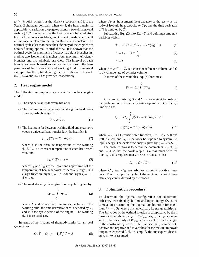
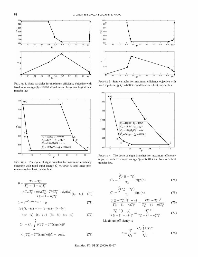
FIGURE 1. State variables for maximum efficiency objective withfixed input energyQ1=10000 kJ and linear phenomenological heattransfer law.

FIGURE 2. The cycle of eight branches for maximum efficiencyobjective with fixed input energyQ1=10000 kJ and linear phe-nomenological heat transfer law.

0 ≈ TnL − Tn

l

TnL − (1− n)Tn

l

+nCmTn

l +nρ0(TnL−Tn

l )Tn−1l sign(n)

TnL−(1− n)Tn

l

(t5′−t4) (70)

1− e−Cm(t5−t5′ ) = µ (71)

t1+(t4−t3) = τ−(τ−t5)−(t5−t5′)

−(t5′−t4)−(t3−t2′)−(t2′−t2)−(t2−t1) (72)

Q1 = CV

τ∫

0

ρ(TnR − Tn)sign(n)θ

× [(TnR − Tn)sign(n)]dt = const (73)

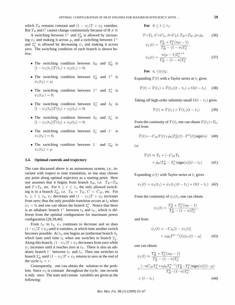
FIGURE 3. State variables for maximum efficiency objective withfixed input energyQ1=6500kJ and Newton’s heat transfer law.

FIGURE 4. The cycle of eight branches for maximum efficiencyobjective with fixed input energyQ1=6500kJ and Newton’s heattransfer law.

Ch =

∧ρ0(Tn

H − Tnh )

Thsign(n) (74)

Cl =

∧ρ0(Tn

L − Tnl )

Tlsign(n) (75)

(TnH − Tn

h )2(1− µ)Tn

H − (1− n)Tnh

=(Tn

L − Tnl )2

TnL − (1− n)Tn

l

(76)

Tn+1h (1− µ)

TnH − (1− n)Tn

h

=Tn+1

l

TnL − (1− n)Tn

l

(77)

Maximum efficiency is

η =W

Q1=

CV

τ∫0

CTdt

Q1(78)

Rev. Mex. Fıs. 55 (1) (2009) 55–67


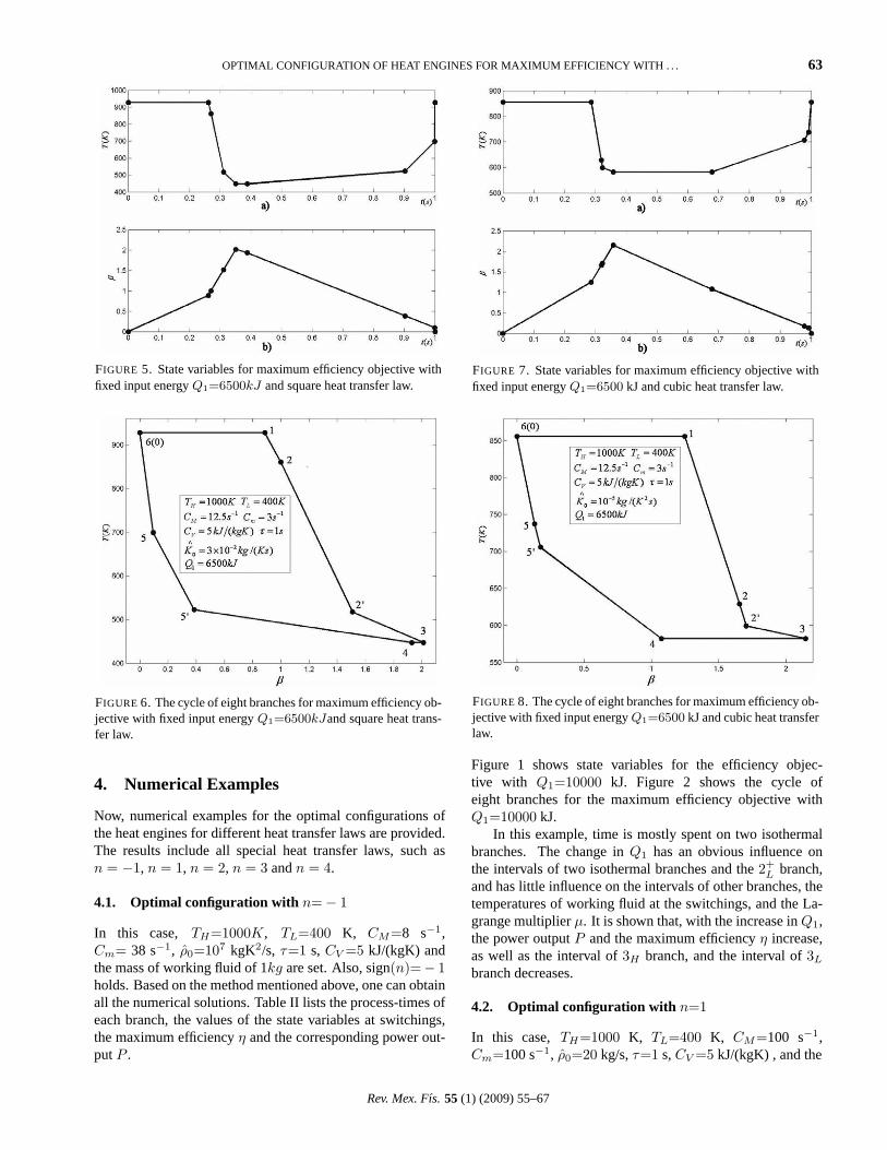
FIGURE 5. State variables for maximum efficiency objective withfixed input energyQ1=6500kJ and square heat transfer law.

FIGURE 6. The cycle of eight branches for maximum efficiency ob-jective with fixed input energyQ1=6500kJand square heat trans-fer law.

4. Numerical Examples

Now, numerical examples for the optimal configurations ofthe heat engines for different heat transfer laws are provided.The results include all special heat transfer laws, such asn = −1, n = 1, n = 2, n = 3 andn = 4.

4.1. Optimal configuration with n=− 1

In this case, TH=1000K, TL=400 K, CM=8 s−1,Cm= 38 s−1, ρ0=107 kgK2/s, τ=1 s, CV =5 kJ/(kgK) andthe mass of working fluid of 1kg are set. Also, sign(n)=− 1holds. Based on the method mentioned above, one can obtainall the numerical solutions. Table II lists the process-times ofeach branch, the values of the state variables at switchings,the maximum efficiencyη and the corresponding power out-putP .

FIGURE 7. State variables for maximum efficiency objective withfixed input energyQ1=6500 kJ and cubic heat transfer law.

FIGURE 8. The cycle of eight branches for maximum efficiency ob-jective with fixed input energyQ1=6500 kJ and cubic heat transferlaw.

Figure 1 shows state variables for the efficiency objec-tive with Q1=10000 kJ. Figure 2 shows the cycle ofeight branches for the maximum efficiency objective withQ1=10000 kJ.

In this example, time is mostly spent on two isothermalbranches. The change inQ1 has an obvious influence onthe intervals of two isothermal branches and the2+

L branch,and has little influence on the intervals of other branches, thetemperatures of working fluid at the switchings, and the La-grange multiplierµ. It is shown that, with the increase inQ1,the power outputP and the maximum efficiencyη increase,as well as the interval of3H branch, and the interval of3L

branch decreases.

4.2. Optimal configuration with n=1

In this case, TH=1000 K, TL=400 K, CM=100 s−1,Cm=100 s−1, ρ0=20 kg/s,τ=1 s,CV =5 kJ/(kgK) , and the

Rev. Mex. Fıs. 55 (1) (2009) 55–67


TABLE IV. Parameters vs.Q1 with square heat transfer law

TH = 1000 K, TL = 400 K, CM = 12.5 s−1, Cm = 3 s−1, CV = 5 kJ/(kgK), ρ0 = 3× 10−2 kg/(Ks),τ = 1 s

Q1 = 6450 kJ Q1 = 6500 kJ Q1 = 6550 kJ

∆t(s) T (K) β ∆t(s) T (K) β ∆t(s) T (K) β

t1 0.2770 929.31 0.8864 0.2611 927.23 0.8859 0.2632 927.90 0.8999

t2 0.0069 877.51 0.9725 0.0091 860.30 0.9992 0.0112 844.45 1.0403

t2′ 0.0419 519.56 1.4966 0.0407 517.16 1.5081 0.0411 505.31 1.5539

t3 0.0409 444.99 2.0073 0.0403 447.01 2.0119 0.0366 447.01 2.0117

t4 0.0211 444.99 1.9629 0.0375 447.01 1.9280 0.0085 447.01 1.9925

t5′ 0.5153 545.23 0.4169 0.5142 522.36 0.3855 0.5397 526.02 0.3736

t5 0.0964 728.07 0.1277 0.0970 698.76 0.0946 0.1015 713.26 0.0691

t6 0.0126 929.31 0 0.0143 927.23 0 0.0142 927.90 0

µ 0.5942 0.5446 0.5424

P 2520.3 kW 2565.7 kW 2592.1 kW

η 0.3848 0.3978 0.3988

mass of working fluid of 1 kg are set. Table III lists theprocess-times of each branch, the values of the state variablesat switchings, the maximum efficiencyη and the correspond-ing power outputP . Figure 3 shows state variables for themaximum efficiency objective withQ1=6500 kJ. Figure 4shows the cycle of eight branches for the maximum efficiencyobjective withQ1=6500 kJ.


In this case, TH=1000 K, TL=400 K, CM=8 s−1,Cm= 8 s−1, ρ0=3 × 10−2 kg/Ks, τ=1 s, CV =5 kJ/(kgK),and the mass of working fluid of 1 kg are set. Table IV liststhe process-times of each branch, the values of the state vari-ables at switchings, the maximum efficiencyη and the cor-responding power outputP . Figure 5 shows state variables

FIGURE 9. State variables for maximum efficiency objective withfixed input energyQ1=6500 kJ and radiative heat transfer law.

for the maximum efficiency objective withQ1=6500 kJ. Fig-ure 6 shows the cycle of eight branches for the maximum ef-ficiency objective withQ1=6500 kJ.

In this example, time is mostly spent on two isothermalbranches. It is shown that, with the increase inρ0, there islittle influence on the temperatures of working fluid at theswitchings and intervals of each branch, and the maximumpower output per cycleP increases, but the correspondingefficiencyη decreases.


In this case, TH=1000 K, TL=400 K, CM=100 s−1,Cm=100 s−1, ρ0 = 10−5 kg/(K2s),τ=1 s,CV =5 kJ/(kgK),and the mass of working fluid of 1 kg are set. Table V lists

FIGURE 10. The cycle of eight branches for maximum efficiencyobjective with fixed input energyQ1 = 6500 kJ and radiative heattransfer law.

Rev. Mex. Fıs. 55 (1) (2009) 55–67


TABLE V. Parameters vs.Q1 with cubic heat transfer law

TH = 1000 K, TL = 400 K, CM = 12.5 s−1, Cm = 3 s−1, CV = 5 kJ/(kgK), ρ0 = 10−5 kg/(K2s),τ = 1 s

Q1 = 6450 kJ Q1 = 6500 kJ Q1 = 6550 kJ


t1 0.2803 853.96 1.2367 0.2865 855.72 1.2484 0.2913 857.27 1.2550

t2 0.0329 626.56 1.6485 0.0326 628.87 1.6557 0.0299 647.71 1.6284

t2′ 0.0054 585.53 1.7163 0.0038 599.401 1.7037 0.0074 590.68 1.7206

t3 0.0424 586.38 2.2463 0.0355 582.30 2.1469 0.0319 574.87 2.1194

t4 0.3332 586.38 1.1016 0.3195 582.30 1.0740 0.3153 574.87 1.0826

t5′ 0.2873 696.41 0.2396 0.2998 705.95 0.1747 0.2916 710.40 0.2079

t5 0.0112 720.17 0.2061 0.0147 737.73 0.1306 0.0260 767.94 0.1300

t6 0.0072 853.96 0 0.0076 855.72 0 0.0132 857.27 0

µ 0.3604 0.3717 0.4098

P 1992.7 kW 2040.0 kW 2239.0 kW

η 0.3042 0.3138 0.3471

TABLE VI. Parameters vs.Q1with radiative heat transfer law

TH = 1000 K, TL = 400K, CM = 12.5 s−1, Cm = 3 s−1, CV = 5 kJ/(kgK), ρ0 = 10−8 kg /(K3 s),τ = 1 s

Q1 = 6450 kJ Q1 = 6500 kJ Q1 = 6550 kJ


t1 0.3378 904.00 1.2385 0.3382 904.00 1.2400 0.3386 904.00 1.2414

t2 0.0166 771.66 1.4458 0.0173 765.71 1.4566 0.0181 759.82 1.4673

t2′ 0.0143 645.35 1.6246 0.0143 640.38 1.6354 0.0143 635.45 1.6461

t3 0.0152 634.00 1.8146 0.0152 634.00 1.8254 0.0152 634.00 1.8361

t4 0.5324 634.00 0.6658 0.5324 634.00 0.6766 0.5324 634.00 0.6873

t5′ 0.0370 654.08 0.5548 0.0370 654.07 0.5656 0.0370 654.06 0.5763

t5 0.0369 730.72 0.4440 0.0369 730.63 0.4549 0.0369 730.54 0.4657

t6 0.0151 904.00 0 0.0158 904.00 0 0.0165 904.00 0

µ 0.0137 0.0137 0.0137

P 3139.3 kW 3166.8 kW 3193.8 kW

η 0.4867 0.4872 0.4876

the process-times of each branch, the values of the state vari-ables at switchings, the maximum efficiencyη and the corre-sponding power outputP . Figure 7 shows state variables formaximum efficiency objective withQ1=6500 kJ. Figure 8shows the cycle of eight branches for the maximum efficiencyobjective withQ1=6500 kJ. The result is similar to that withn=2.


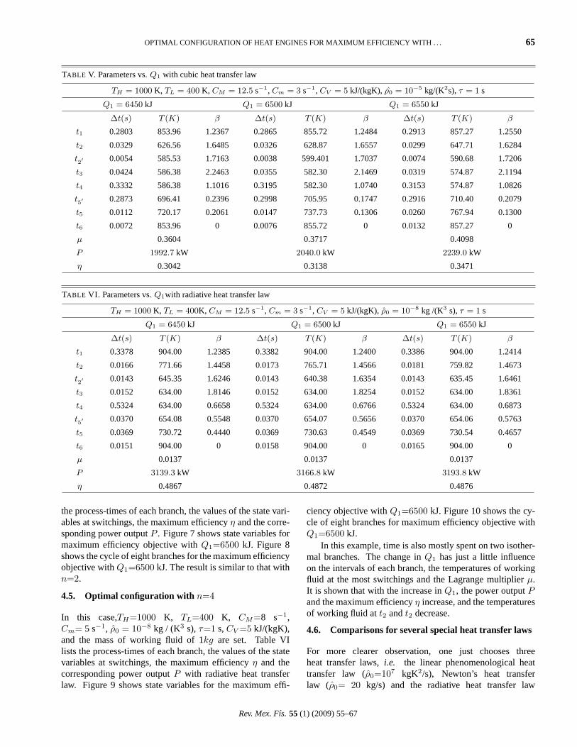
In this case,TH=1000 K, TL=400 K, CM=8 s−1,Cm= 5 s−1, ρ0 = 10−8 kg / (K3 s),τ=1 s,CV =5 kJ/(kgK),and the mass of working fluid of 1kg are set. Table VIlists the process-times of each branch, the values of the statevariables at switchings, the maximum efficiencyη and thecorresponding power outputP with radiative heat transferlaw. Figure 9 shows state variables for the maximum effi-

ciency objective withQ1=6500 kJ. Figure 10 shows the cy-cle of eight branches for maximum efficiency objective withQ1=6500 kJ.

In this example, time is also mostly spent on two isother-mal branches. The change inQ1 has just a little influenceon the intervals of each branch, the temperatures of workingfluid at the most switchings and the Lagrange multiplierµ.It is shown that with the increase inQ1, the power outputPand the maximum efficiencyη increase, and the temperaturesof working fluid att2 andt2 decrease.

4.6. Comparisons for several special heat transfer laws

For more clearer observation, one just chooses threeheat transfer laws,i.e. the linear phenomenological heattransfer law (ρ0=107 kgK2/s), Newton’s heat transferlaw (ρ0= 20 kg/s) and the radiative heat transfer law

Rev. Mex. Fıs. 55 (1) (2009) 55–67


FIGURE 11. Optimal temperature of working fluid vs. time formaximum efficiency objective with three heat transfer laws.

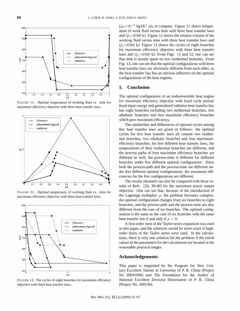
FIGURE 12. Optimal temperature of working fluid vs. time formaximum efficiency objective with three heat transfer laws.

FIGURE 13. The cycles of eight branches for maximum efficiencyobjective with three heat transfer laws.

(ρ0=10−8 kg/(K3 s)), to compare. Figure 11 shows temper-ature of work fluid versus time with three heat transfer lawsandQ1=6500 kJ. Figure 12 shows the relative volume of theworking fluid versus time with three heat transfer laws andQ1=6500 kJ. Figure 13 shows the cycles of eight branchesfor maximum efficiency objective with three heat transferlaws andQ1=6500 kJ. From Figs. 11 and 12, one can seethat time is mostly spent on two isothermal branches. FromFig. 13, one can see that the optimal configurations with threeheat transfer laws are obviously different from each other, sothe heat transfer law has an obvious influence on the optimalconfigurations of the heat engines.

5. Conclusion

The optimal configuration of an endoreversible heat enginefor maximum efficiency objective with fixed cycle period,fixed input energy and generalized radiative heat transfer lawhas eight branches including two isothermal branches, twoadiabatic branches and four maximum efficiency brancheswhich give maximum efficiency.

The similarities and differences of optimal cycles amongfive heat transfer laws are given as follows: the optimalcycles for five heat transfer laws all contain two isother-mal branches, two adiabatic branches and four maximum-efficiency branches; for five different heat transfer laws, thetemperatures of their isothermal branches are different, andthe process paths of four maximum efficiency branches aredifferent as well; the process-time is different for differentbranches under five different optimal configuration. Sinceboth the process-path and the process-time are different un-der five different optimal configurations, the maximum effi-ciencies for the five configurations are different.

The results obtained can also be compared with those re-sults of Refs. [26, 38-40] for the maximum power outputobjective. One can see that, because of the introduction ofthe Lagrange multiplierµ, the problem becomes complex,the optimal configuration changes from six branches to eightbranches, and the process-path and the process-time are alsodifferent from the case of six branches. The optimal config-uration is the same as the case of six branches with the sameheat transfer law if and only ifµ = 0.

A first-order item of the Taylor series expansion was usedin this paper, and the solutions would be more exact if high-order items of the Taylor series were used. In the calcula-tions, there is only one solution for the problem if the initialvalues of the parameters for the calculations are located in thereasonable practical ranges.

Acknowledgements

This paper is supported by the Program for New Cen-tury Excellent Talents in University of P. R. China (ProjectNo 20041006) and The Foundation for the Author ofNational Excellent Doctoral Dissertation of P. R. China(Project No. 200136).

Rev. Mex. Fıs. 55 (1) (2009) 55–67


1. B. AndresenFinite-Time Thermodynamics. (Physics Labora-tory II, University of Copenhagen, 1983).

2. B. Andresen, P. Salamon, and R.S. Berry,Phys. Today(1984)62.

3. B. Andresen, R.S. Berry, M.J. Ondrechen, and P. Salamon,(Acc. Chem. Res.(1984) 266.

4. S. Sieniutycz and P. Salamon,Advances in Thermodynamics.“Finite Time Thermodynamics and Thermoeconomics” (NewYork: Taylor Francis, 1990)4.

5. D.C. Agrawal and V.J. Menon,Eur. J. Phys.11 (1990) 305.

6. D.C. Agrawal and V.J. Menon,J. Appl. Phys.74 (1993) 2153.

7. D.C Agrawal, J.M Gordon, and M. Huleihil,Indian J. Engng.Mater. Sci.1 (1994) 195.

8. S. Sieniutycz and J.S. Shiner,J. Non-Equilib. Thermodyn.(1994) 303.

9. A. Bejan,J. Appl. Phys.79 (1996) 1191.

10. K.H Hoffmann, J.M Burzler, and S. Schubert,J. Non- Equilib.Thermodyn.22 (1997) 311.

11. R.S Berry, V.A Kazakov, S. Sieniutycz, Z. Szwast, and A.M.Tsirlin Thermodynamic Optimization of Finite Time Processes.(Chichester: Wiley, 1999).

12. L. Chen, C. Wu, and F. Sun,J. Non-Equilib. Thermodyn.24(1999) 327.

13. P. Salamon, J.D. Nulton, G. Siragusa, T.R Andresen, and A.Limon Energy, The Int. J.26 (2001) 307.

14. D. Ladino-Luna,Rev. Mex. Fıs.48 (2002) 575.

15. S. Sieniutycz, “Thermodynamic limits on production or con-sumption of mechanical energy in practical and industry sys-tems.”Progress Energy Combustion Science29 (2003) 193.

16. K.H. Hoffman, J. Burzler, A. Fischer, M. Schaller, and S. Schu-bert, J. Non-Equilib. Thermodyn.28 (2003) 233.

17. L. Chen, F. Sun,Advances in Finite Time Thermodynamics:Analysis and Optimization.(New York: Nova Science Publish-ers, 2004.)

18. L. Chen, Finite time thermodynamic analysis of irreversibleprogresses and cycles.(Beijing: High Education Press,(in Chi-nese), 2005).

19. S. Sieniutycz and H. Farkas,Variational and Extremum Princi-ples in Macroscopic Systems.(London: Elsevier Science Pub-lishers, 2005).

20. D. Ladino-Luna and R.P. Paez-Hernandez,Rev. Mex. Fıs., 51(2005) 54.

21. G. Aragon-Gonzalez, A. Canales-Palma, A. Lenon-Galicia, andM. Musharrafie-Martinez,Rev. Mex. Fıs.51 (2005) 32.

22. C.A Herrera, M.E Rosillo, and L. CastanoRev. Mex. Fıs. 54(2008) 118.

23. G. Aragon-Gonzalez, A. Canales-Palma, A. Leon-Galicia, andJ.R. Morales-Gomez,Brazilian J. Physics, 38 (2008) 1.

24. D. Cutowicz-Krusin, J. Procaccia, and J. Ross,J. Chem. Phys.69 (1978) 3898.

25. F.L. Curzon , B. Ahlborn,Am. J. Phys.43 (1975) 22.

26. M.H. Rubin,Phys. Rev. A.19 (1979) 1272.

27. M.H. Rubin,Phys. Rev. A.22 (1980) 1741.

28. A. De Vos,Am. J. Phys.53 (1985) 570.

29. A. De Vos,J. Phys. D: Appl. Phys.20 (1987) 232.

30. L. Chen, Z. Yan,J. Chem. Phys.90 (1989) 3740.

31. J.M. Gordon,Am. J. Phys.58 (1990) 370.

32. D. Ladino-Luna,Rev. Mex. Fıs.49 (2003) 87.

33. L. Chen, F. Sun, and C. Wu,J. Phys. D: App. Phys.32 (1999)99.

34. L. Chen, X. Zhu, F. Sun, and C. Wu,Appl. Energy78 (2004)305.

35. S. Sieniutycz, and P. Kuran,Int. J. Heat Mass Transfer48(2005) 719.

36. S. Sieniutycz, and P. Kuran,Int. J. Heat Mass Transfer, 49(2006) 3264.

37. M.A. Barranco-Jimenez, N. Sanchez-Salas, and F. Angulo-Brown,Rev. Mex. Fıs.54 (2008) 284.

38. H. Song, L. Chen, J. Li, and C. Wu,J. Appl. Phys.100 (2006)124907.

39. H. Song, L. Chen,and F. Sun,Appl. Energy84 (2007) 374.

40. J. Li, L. Chen,and F.Sun,Applied Energy84 (2007) 944.

41. H.B Callen ,Thermodynamics and an Introduction to Thermo-statics.(New York: Wiley, 1985).

Rev. Mex. Fıs. 55 (1) (2009) 55–67

optimal conﬁguration of heat engines for maximum efﬁciency ... · obeys other laws; heat...

Documents