LESA˙165685 703xml April 18, 2006 16:16

Optimal Calibration Methodfor Water Distribution WaterQuality Model

QUERY SHEET

0

LESA˙165685 703xml April 18, 2006 16:16

Journal of Environmental Science and Health Part A, 41:1–16, 2006Copyright C© Taylor & Francis Group, LLCISSN: 1093-4529 (Print); 1532-4117 (Online)DOI: 10.1080/10934520600657115

Optimal Calibration Method1

for Water Distribution Water2

Quality Model3

Zheng Yi Wu4

Bentley Systems, Incorporated, Haestad Methods Solution Center, Watertown,5CT, USA6

A water quality model is to predict water quality transport and fate throughout a7water distribution system. The model is not only a promising alternative for analyzing8disinfectant residuals in a cost-effective manner, but also a means of providing9enormous engineering insights into the characteristics of water quality variation and10constituent reactions. However, a water quality model is a reliable tool only if it predicts11what a real system behaves. This paper presents a methodology that enables a modeler12to efficiently calibrate a water quality model such that the field observed water quality13values match with the model simulated values. The method is formulated to adjust14the global water quality parameters and also the element-dependent water quality15reaction rates for pipelines and tank storages. A genetic algorithm is applied to optimize16the model parameters by minimizing the difference between the model-predicted17values and the field-observed values. It is seamLessly integrated with a well-developed18hydraulic and water quality modeling system. The approach has provided a generic19tool and methodology for engineers to construct the sound water quality model in20expedient manner. The method is applied to a real water system and demonstrated21that a water quality model can be optimized for managing adequate water supply to22public communities.23

Key Words: Water distribution; Water supply; Water quality model; Chlorine decay;24Simulation; Calibration; Optimization; Genetic algorithm.25

INTRODUCTION26

Drinking water quality is essential to public heath. Although water treatment27is a common practice for supplying good quality of water from a source,28maintaining an adequate water quality throughout a distribution system29is a daunting task. The challenges remain in the complex pipe geometry,30

Address correspondence to Zheng Yi Wu, Bentley Systems Inc., Haestad MethodsSolution Center, 27 Siemon Company Drive, Suite 200W, Watertown CT06795, USA;E-mail: Zheng.Wu@bentley.com

1

LESA˙165685 703xml April 18, 2006 16:16

2 Wu

sophisticated network connectivity, various system operation controls, tem-31poral and spatial variation of water demand, and also intriguing constituent32reaction in bulk water and in between the water and pipe walls. Sampling33and continuously monitoring water quality at appropriate locations have34played an important role to minimize the risk of inadequate water quality35to public health, however, but sampling only presents a limited picture of36water quality in that there are only a few monitoring points and mon-37itoring cannot be used to predict future conditions or perform “what if”38analyses due to the limited coverage and the high cost. Thus, using a well-39developed hydraulic and water quality model is an important approach for40simulating the hydraulic and water quality dynamics for all elements in a41system.42

Water quality modeling has become an increasingly common practice for43water utilities around world. It is formulated as a mathematical model and44developed as computer-based tool to predict water quality transport and fate45within a water distribution system according to the network flow dynamics.46The model is not only a promising technology for predicting disinfectant47residuals in a cost-effective manner, but also a means of providing enormous48engineering understanding in the dynamics of water quality variation and the49sophisticated process of constituent reactions that occur in water distribution50systems. The early development of water quality models was based upon the51steady-state hydraulic simulation of mass conservation law. The models[1–4]52determined the water quality spatial distribution of a constituent throughout53a pipeline network under static hydraulic conditions.54

Although the steady-state water quality model proved to be useful for55investigating the overall movement of a contaminant under constant con-56ditions, the system hydraulics is constantly changing in tank levels, valve57settings, pump operating status and nodal demand. Therefore, the need for58the models that represent the dynamics of contaminant movement led to59the development of better water quality models under temporally varying60conditions. Dynamic models of water quality in distribution systems explicitly61take into account of changing in flows through pipelines and storage facilities62over an extended period of time. A number of solution methods[5–9] are63developed for dynamic water quality models. They can be classified spatially as64either Eulerian or Lagrangian and temporally as time-driven or event-driven65methods. Each of these methods assumes that a hydraulic model determines66the flow direction and velocity in each pipe at specific time intervals over an67extended period. Within each interval, referred as hydraulic time step, the pipe68flow velocity remains constant, the simulation of a constituent movement and69reaction proceeds in a smaller time step (so-called water quality time step).70Thus the dynamic approach is more realistic than steady-state methods in71simulating systematic condition of water quality transportation and reaction72in distribution networks.73

LESA˙165685 703xml April 18, 2006 16:16

Model to Predict Water Quality Transport 3

However, a water quality model is an effective and reliable analysis tool74only when the constituent reaction and decay/growth mechanisms are properly75defined. This can only be achieved by calibrating the water quality model using76the field observed and lab-tested water quality data. Like hydraulic model77calibration, water quality model calibration is a time-consuming and tedious78process by manually adjusting model parameters. In this article, a competent79genetic algorithm-based calibration approach for calibrating a water quality80model is presented. It provides modelers a flexible optimization modeling tool81to facilitate the water quality model calibration task. In order to develop an82effective calibration method, it is important to understand the insights into83water quality model formulation. A brief overview of water quality model is84given next.85

WATER QUALITY MODEL86

Water quality model for a water distribution system is based upon Reynolds87transport theorem (RTT) and formulated for one-dimensional, unsteady small88fluid parcel as follows.89

∂C∂t

+ V∂C∂x

= R(C) (1)

90 where C is the concentration of a constituent; t is time; V is the flow velocity;91x is the distance and R represents the constituent reaction relationship. Water92quality model for a water distribution system used in this paper is based93upon a parcel tracking algorithm.[8,9] It tracks the change in water quality94of discrete parcels of water as they move along pipes and mixes together at95junctions between fixed-length time steps. During a simulation, the water96quality in each parcel is updated to reflect any reaction that may have occurred97over the time step. The water from the leading parcels of pipes with flow98into each junction is blended together, along with any external inflow to the99junction, to compute a new water quality value at the junction. The volume100contributed from each parcel equals the product of its pipe’s flow rate and the101time step. If this volume exceeds that of the leading parcel then the leading102parcel is destroyed and the next parcel in line behind it begins to contribute its103volume. New parcels are created in pipes with flow out of each junction. The104parcel volume equals the product of the pipe flow and the time step.105

To reduce on the number of parcels, a new parcel is formed if the new106junction quality differs by a user-specified tolerance from that of the last parcel107in the outflow pipe. If the difference in quality is below the tolerance then the108size of the last parcel is simply increased by the volume of flow released into109the pipe over the time step with no change in quality. Initially each pipe in110the network consists of a single parcel whose quality equals the initial quality111assigned to the upstream node. The water quality simulation tracks the growth112

LESA˙165685 703xml April 18, 2006 16:16

4 Wu

or decay of a substance by reaction as it travels through a distribution system.113To do this, it needs to know the rate at which the substance reacts and how114this rate might depend on substance concentration. Reactions can occur both115within the bulk flow and with material along the pipe wall. Bulk fluid reactions116can also occur within tanks.117

Bulk Reaction118

Bulk flow reactions are the reactions that occur in the main flow stream119of a pipe or in a storage tank, unaffected by any processes that might120involve the pipe wall. A water quality model simulates these reactions using121n-th order kinetics, where the instantaneous rate of reaction (R in unit of122mass/volume/time) is assumed to be concentration-dependent, given as:123

R(C) = KbCn (2)

124 where Kb is a bulk rate coefficient; C is reactant concentration (mass/volume)125and n is a reaction order. Kb has units of concentration raised to the (1−n)126power divided by time. It is positive for growth reactions and negative for decay127reactions. It also considers reactions where a limiting concentration exists on128the ultimate growth or loss of the substance. In this case the rate expression129for a growth reaction becomes130

R(C) = Kb(CL − C)C(n−1) (3)

131 where CL = the limiting concentration. For decay reactions (CL−C) is replaced132by (C−CL).133

Thus, there are three parameters (Kb, CL, and n) that are used to134characterize bulk reaction rates. Different values of these parameters lead to135different kinetic models. They need to be carefully calibrated for the pipes and136tanks in a water distribution system.137

Wall Reaction138

In addition to bulk flow reactions, constituent reactions occur with mate-139rial on or near the pipe wall. The rate of this reaction is dependent on the140concentration in the bulk flow and pipe wall conditions, given as:141

R(C) = (A/V)KwCn (4)

142 Where Kw is a wall reaction rate coefficient and (A/V) is the surface area per143unit volume within a pipe. It converts the mass reacting per unit of wall area144to a per unit volume basis. n is the wall reaction order taking value of either1450 or 1, so that the unit of Kw is either mass/area/time or length/time. Both Kw146and n are site specific and need to be calibrated for water distribution pipes.147

LESA˙165685 703xml April 18, 2006 16:16

Model to Predict Water Quality Transport 5

CALIBRATION FORMULATION148

To calibrate a water quality model for analyzing any constituent (not just Chlo-149rine decay), it is important to adjust the parameters that govern the reaction150mechanism. It includes bulk reaction and pipe wall reaction parameters.151

Bulk Water Reaction Calibration152

Bulk reaction rate is conventionally obtained by conducting bottle test153in a laboratory, namely taking bottles of sample water and measuring the154constituent concentration of the bottle water over time test to determine the155bulk water reaction rate. For chlorine decay, one can measures the residual156of chlorine over time, so that bulk reaction/decay can be gauged by the bottle157test. Bottle test is recommended for determining the bulk reaction coefficient158such as chlorine decay factor. It provides a good baseline value and reference159for constructing a water quality model. Although bulk reaction coefficient can160be attained by bottle test, real bulk reaction may vary from one portion of a161system to another due to dynamic flow conditions and mixing of multiple water162sources. The real bulk reaction mechanism needs to be calibrated throughout163a distribution system. Bulk water reaction is generally characterized by three164parameters including:165

(i) Bulk reaction coefficient Kb;166(ii) Bulk reaction order nb;167(iii) Concentration limit CL.168

Bulk reaction parameters need to be adjusted for both pipe and tank169elements. The pipes that are of the similar characteristics are allowed to be170grouped into one calibration group for bulk reaction coefficient adjustment.171The bulk reaction groups are set up in a similar fashion to the roughness172group,[10] prescribed with minimum, maximum values and an increment for173each pipe group and tank. The same reaction parameters are applied to the174pipes in one calibration group. This reduces the number of the calibration175parameters. Tank bulk reaction coefficient is calibrated individually for each176storage facility. By adjusting all the parameters (Kb, nb and CL), a water177quality model can be calibrated to simulate the bulk water reaction of not178only chlorine decay, but also the other reaction mechanisms such as first-179order saturation growth, two-component second-order growth, two-component180second-order decay and the other reaction mechanisms.181

Pipe Wall Reaction Calibration182

Pipe wall reaction is characterized by the wall coefficient (Kw) and reaction183order (nw). Both parameters are closely related to pipe material and pipe wall184

LESA˙165685 703xml April 18, 2006 16:16

6 Wu

physical conditions such as encrustation and tuburculation of corrosion prod-185ucts. Two methods are developed for calibrating pipe wall reaction mechanism.186

Direct Calibration187

Direct calibration is to directly optimize the pipe wall reaction coefficient188and reaction order for a group of pipes. Since the wall reaction mechanism is189expected to have the same behavior for the pipes of the same characteristics190(age, material and location). Similar to the roughness calibration group,[11]191pipes of the same characteristics are allowed to be aggregated and treated as a192set of common calibration parameters, wall coefficient and order are calibrated193between the minimum and maximum values with an increment specified by a194modeler.195

Correlation Calibration196

Alternatively, pipe wall reaction can be calibrated by adjusting a corre-197lation factor. It is well known that as metal pipes age their roughness tends198to increase due to encrustation and tuburculation of corrosion products on199the pipe walls. This increase in roughness produces a lower Hazen-Williams200C-factor or a higher Darcy-Weisbach roughness coefficient, resulting in greater201frictional headloss in flow through the pipe. There is some evidence[12] to202suggest that the same processes that increase a pipe’s roughness with age also203tend to increase the reactivity of its wall with some chemical species, particu-204larly chlorine and other disinfectants. Each pipe’s wall reaction coefficient (Kw)205can be a function of the coefficient used to describe its roughness. A different206function applies depending on the formula used to compute headloss through207a pipe:208

Hazen–Williams: Kw = F/C (5)

Darcy–Weisbach: Kw = −F/ log(e/d) (6)

Chezy–Manning: Kw = F∗N (7)

209 where C is Hazen–Williams C-factor; e is Darcy-Weisbach roughness, d is210pipe diameter, N is Manning roughness coefficient and F is the coefficient211of correlation of wall reaction and pipe roughness. The coefficient F must212be developed from site-specific field measurements and will have a different213meaning depending on which headloss equation is used. The advantage of214using this approach is that it requires only a single parameter F, to allow wall215reaction coefficients to vary throughout the network in a physically meaningful216way. This is because a hydraulic model must be calibrated before undertaking a217water quality model calibration. Therefore, pipe roughness should be a known218value for water quality model calibration. In this case, modelers may choose to219

LESA˙165685 703xml April 18, 2006 16:16

Model to Predict Water Quality Transport 7

just calibrate the correlation factor for Chlorine pipe wall reaction mechanism.220Correlation factor adjustment can also be conducted for a group of pipes or221globally for an entire system.222

One calibration solution represents one set of parameters that define223the bulk water reaction and pipe wall reaction mechanism. Each possible224solution is passed to a hydraulic and water quality model which produces the225simulation results of water quality concentrations in a system. The simulated226concentration values are compared with the observed values. The comparison227is quantified as a goodness-of-fit between the simulated and the observed228values. The goodness-of-fit is defined as a fitness or calibration objective229function in the following section.230

Calibration Objectives231

The objective of water quality model calibration is to minimize the232difference between the field observed and the model simulated constituent233concentrations. Assume the field observed concentration be represented by234Ci

obs(tj) at time tj for monitoring location i and collected over N time steps235at M locations while the model simulated concentration is noted as Ci

sim(tj).236The calibration objective can be measured in many different ways formulated237as follows.238

Minimize difference square:239

Fitness =∑M

i=1∑N

j=1

(Cobs

i (tj ) − Csimi (tj )

)2

N × M(8)

240Minimize absolute difference:241

Fitness =∑N

i=1∑M

j=1

∣∣Cobsi (tj ) − Csim

i (tj )∣∣

N × M(9)

242Minimize absolute maximum difference:243

Fitness = maxi,j

∣∣Cobsi (tj ) − Csim

i (tj )∣∣ (10)

244Minimize sum of absolute mean difference:245

Fitness =M∑

i=1

∑Nj=1

∣∣Cobsi (tj ) − Csim

i (tj )∣∣

N(11)

246When chemical concentration is collected at a sampling/monitoring station, it247may not be measured at a regular time step. To compare between the observed248and simulated concentration, the simulated result must be obtained for the249same time as the observed value is collected. When the simulation time step250

LESA˙165685 703xml April 18, 2006 16:16

8 Wu

does not exactly match the time step of data collection, the simulated concen-251tration is attained by interpolating the results at two adjacent computation252time steps for the same monitor location/node. The coefficients for bulk water253and pipe wall reaction can be calibrated for pipe groups while the reaction254orders and concentration limit are global parameters for a system.255

Water quality calibration, formulated as above, is a nonlinear implicit256optimization problem. It is solved by using the same methodology for hydraulic257model calibration by Wu et al.[10,11] In fact, the hydraulic calibration has been258extended to include the calibration of water quality parameters by means of259the competent genetic algorithm.[13]260

SOLUTION METHODOLOGY261

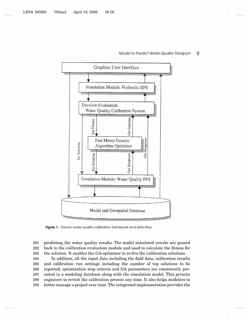
The implementation of water quality calibration algorithm is illustrated in262Figure 1. The information flows in both directions between the end-user and263the data storage and thus enables engineers to effectively manage the data and264calibrate a model by exploiting the powerful combination of GA optimizer and265hydraulic network simulator, both are embodied into one modeling system.266It consists of a user interface, calibration evaluation module, GA optimizer,267hydraulic and water quality simulation model.268

A user interface on a personal computer or other workstation lends the269user the ability to enter the field observed data, select the representative de-270mand loading, corresponding boundary conditions (including pump operating271status, valve settings and tank levels) and calibration criteria. It enables a272modeler to intuitively set up calibration, persistently conducting calibration273tasks and graphically presenting results.274

An initial calibration model is established by performing the extended pe-275riod hydraulic simulation. The results are saved in the file that is repetitively276used for water quality analysis of each calibration solution. A calibration run277may proceed by either interactively adjusting calibration parameters (manu-278ally set a value for each parameter), that is to bypass the genetic algorithm279optimizer, or presenting the data to GA optimizer to automatically search280for the optimal and near optimal calibration solutions. Without activating281the GA optimizer, the user-estimated model parameters are submitted to the282hydraulic and water quality simulator. It predicts the water quality responses283that are passed back to calibration evaluation module. The goodness-of-fit is284calculated and reported to a user. Modelers can estimate the parameters and285iterate over the process to enhance model calibration. In contrast, calibration286can proceed with GA optimizer searching for the optimal solution. The GA287optimizer will automatically generate and optimize the calibration solutions.288Each trial solution, along with the selected data sets, corresponding loading289and boundary conditions, is submitted to hydraulic network simulator for290

LESA˙165685 703xml April 18, 2006 16:16

Model to Predict Water Quality Transport 9

Figure 1: Darwin water quality calibration framework and data flow.

predicting the water quality results. The model simulated results are passed291back to the calibration evaluation module and used to calculate the fitness for292the solution. It enables the GA-optimizer to evolve the calibration solutions.293

In addition, all the input data including the field data, calibration results294and calibration run settings including the number of top solutions to be295reported, optimization stop criteria and GA parameters are consistently per-296sisted in a modeling database along with the simulation model. This permits297engineers to revisit the calibration process any time. It also helps modelers to298better manage a project over time. The integrated implementation provides the299

LESA˙165685 703xml April 18, 2006 16:16

10 Wu

powerful features of hydraulic and water quality network modeling paradigm.300It has been applied to the optimization of the water quality model for chlorine301decay study by Vasconcelos et al.[12]302

CASE STUDY303

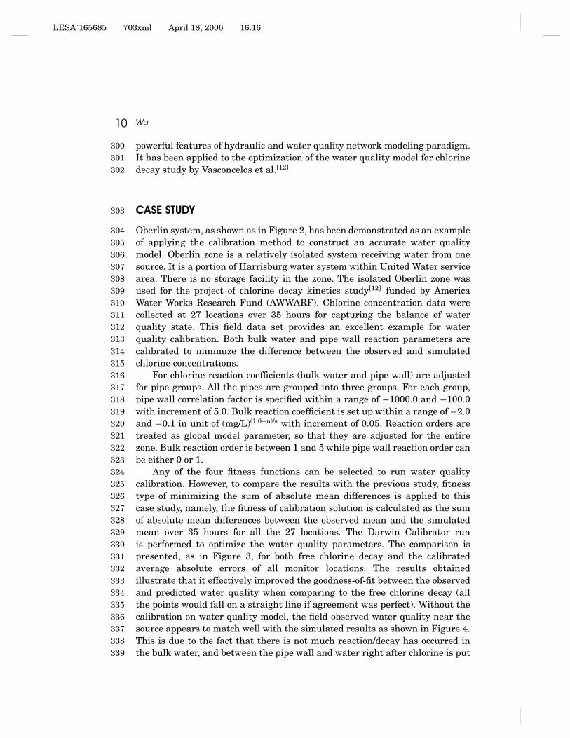
Oberlin system, as shown as in Figure 2, has been demonstrated as an example304of applying the calibration method to construct an accurate water quality305model. Oberlin zone is a relatively isolated system receiving water from one306source. It is a portion of Harrisburg water system within United Water service307area. There is no storage facility in the zone. The isolated Oberlin zone was308used for the project of chlorine decay kinetics study[12] funded by America309Water Works Research Fund (AWWARF). Chlorine concentration data were310collected at 27 locations over 35 hours for capturing the balance of water311quality state. This field data set provides an excellent example for water312quality calibration. Both bulk water and pipe wall reaction parameters are313calibrated to minimize the difference between the observed and simulated314chlorine concentrations.315

For chlorine reaction coefficients (bulk water and pipe wall) are adjusted316for pipe groups. All the pipes are grouped into three groups. For each group,317pipe wall correlation factor is specified within a range of −1000.0 and −100.0318with increment of 5.0. Bulk reaction coefficient is set up within a range of −2.0319and −0.1 in unit of (mg/L)(1.0−n)/s with increment of 0.05. Reaction orders are320treated as global model parameter, so that they are adjusted for the entire321zone. Bulk reaction order is between 1 and 5 while pipe wall reaction order can322be either 0 or 1.323

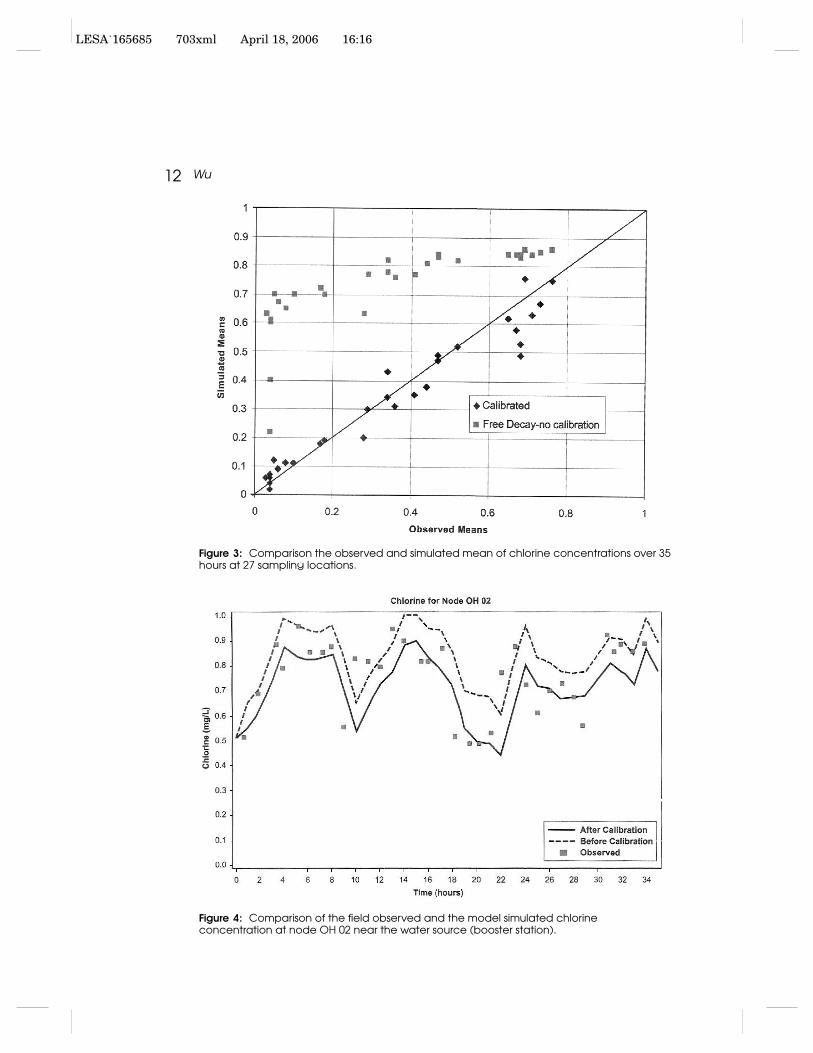
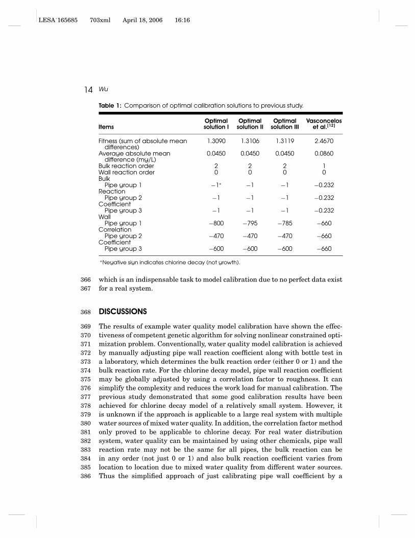
Any of the four fitness functions can be selected to run water quality324calibration. However, to compare the results with the previous study, fitness325type of minimizing the sum of absolute mean differences is applied to this326case study, namely, the fitness of calibration solution is calculated as the sum327of absolute mean differences between the observed mean and the simulated328mean over 35 hours for all the 27 locations. The Darwin Calibrator run329is performed to optimize the water quality parameters. The comparison is330presented, as in Figure 3, for both free chlorine decay and the calibrated331average absolute errors of all monitor locations. The results obtained332illustrate that it effectively improved the goodness-of-fit between the observed333and predicted water quality when comparing to the free chlorine decay (all334the points would fall on a straight line if agreement was perfect). Without the335calibration on water quality model, the field observed water quality near the336source appears to match well with the simulated results as shown in Figure 4.337This is due to the fact that there is not much reaction/decay has occurred in338the bulk water, and between the pipe wall and water right after chlorine is put339

LESA˙165685 703xml April 18, 2006 16:16

Model to Predict Water Quality Transport 11

Figure 2: Oberlin zone of Harrisburg Water Distribution System.

into the system at the source (booster station in this case). Water quality at340the outskirt of the system, however, is quite different from the nodes near the341pump station. Figure 5 implies that significant chlorine decay has taken place342from the source into the distribution system. Without good calibration on the343water quality model, the field observed chlorine residual is away mismatched344with the model simulated. Figures 3 and 5 demonstrate that the calibration345

LESA˙165685 703xml April 18, 2006 16:16

12 Wu

Figure 3: Comparison the observed and simulated mean of chlorine concentrations over 35hours at 27 sampling locations.

Figure 4: Comparison of the field observed and the model simulated chlorineconcentration at node OH 02 near the water source (booster station).

LESA˙165685 703xml April 18, 2006 16:16

Model to Predict Water Quality Transport 13

Figure 5: Comparison of the field observed and the model simulated chlorineconcentration at node OH 24 the outskirt of system.

approach successfully enhances the chlorine residual agreement, particularly346for the nodes far apart from the source.347

Three top calibration solutions are presented in Table 1 and compared with348previous study. The best fitness of 1.309 with average difference of 0.045 mg/L349has been achieved for 27 sampling stations over 35 hours while the previous350study resulted in the fitness of 2.467 with average of 0.086 mg/L. It clearly351indicates that the better calibration solutions have been obtained by using the352optimal calibration method. The solutions are ranked by the fitness value, the353sum of absolute mean differences, which is resulted in by different correlation354factor between pipe wall coefficient and roughness for pipe groups. The average355of absolute mean differences is the same for all three solutions. It is no356doubt that genetic algorithm calibration effectively improved the water quality357model for this case study and a better solution has been obtained than the358conventional approach. However, an accurate water quality model cannot be359expected to be achieved by simply performing optimization calibration run. An360insightful analysis must be undertaken for understanding the solution and361the data points where the relatively greater discrepancies are resulted in. This362is usually caused by poor data quality and abnormal model representation.363Optimization modeling tool may help engineers quickly to reveal the weakest364where good engineering judgment is applied to investigate the possible errors,365

LESA˙165685 703xml April 18, 2006 16:16

14 Wu

Table 1: Comparison of optimal calibration solutions to previous study.

ItemsOptimalsolution I

Optimalsolution II

Optimalsolution III

Vasconceloset al.[12]

Fitness (sum of absolute meandifferences)

1.3090 1.3106 1.3119 2.4670

Average absolute meandifference (mg/L)

0.0450 0.0450 0.0450 0.0860

Bulk reaction order 2 2 2 1Wall reaction order 0 0 0 0Bulk

Pipe group 1 −1∗ −1 −1 −0.232Reaction

Pipe group 2 −1 −1 −1 −0.232Coefficient

Pipe group 3 −1 −1 −1 −0.232Wall

Pipe group 1 −800 −795 −785 −660Correlation

Pipe group 2 −470 −470 −470 −660Coefficient

Pipe group 3 −600 −600 −600 −660

∗Negative sign indicates chlorine decay (not growth).

which is an indispensable task to model calibration due to no perfect data exist366for a real system.367

DISCUSSIONS368

The results of example water quality model calibration have shown the effec-369tiveness of competent genetic algorithm for solving nonlinear constrained opti-370mization problem. Conventionally, water quality model calibration is achieved371by manually adjusting pipe wall reaction coefficient along with bottle test in372a laboratory, which determines the bulk reaction order (either 0 or 1) and the373bulk reaction rate. For the chlorine decay model, pipe wall reaction coefficient374may be globally adjusted by using a correlation factor to roughness. It can375simplify the complexity and reduces the work load for manual calibration. The376previous study demonstrated that some good calibration results have been377achieved for chlorine decay model of a relatively small system. However, it378is unknown if the approach is applicable to a large real system with multiple379water sources of mixed water quality. In addition, the correlation factor method380only proved to be applicable to chlorine decay. For real water distribution381system, water quality can be maintained by using other chemicals, pipe wall382reaction rate may not be the same for all pipes, the bulk reaction can be383in any order (not just 0 or 1) and also bulk reaction coefficient varies from384location to location due to mixed water quality from different water sources.385Thus the simplified approach of just calibrating pipe wall coefficient by a386

LESA˙165685 703xml April 18, 2006 16:16

Model to Predict Water Quality Transport 15

correlation factor is unlikely be able to handle all the complexity of a real water387quality model. In contrast, the water quality calibration approach developed388in this paper is generic and flexible method taking into account combination389of different water quality parameters. It is able to consider the element-390dependent reaction parameters (for both pipe and tank) and any reaction order.391With the capability of grouping the pipes of similar characteristics, modeler is392able to calibrate a water quality model of any constituent.393

To achieve a good water quality calibration, a well calibrated EPS394hydraulic model is essential before starting water quality calibration. The395accuracy of water quality simulation relies on the hydraulic simulation results.396A hydraulic simulation must be performed priori to a water quality analysis.397It is the hydraulic simulation that provides the necessary flow and velocity398information of each element to determine how a constituent is transported399and reacted throughout a distribution system. This indicates that hydraulic400calibration must be conducted before embarking on water quality model401calibration, and also hydraulic model calibration must be carried out for402extended period simulation. If there are errors in the hydraulic model, then403forcing the water quality parameters to achieve calibration may result in a404model that appears calibrated due to compensating errors.405

CONCLUSIONS406

Water quality modeling is an important means of providing system-wide infor-407mation on water quality for evaluating routine system operation policy, thus408maintaining and improving water quality throughout a system. Calibrating409such a model ensures that a water quality model predicts what is happening410in a real system. The approach presented in this paper has provided a generic411tool and methodology for calibrating a water quality model of any constituent.412It relieves modeler from trial and error process and thus enables engineers413to construct an accurate model for effectively managing water quality in414distribution systems to comply the public health.415

ACKNOWLEDGMENT416

Author would like to thank Dr. Walter Grayman and Dr. Lewis Rossman for417providing the data used for this research.418

REFERENCES419

1. Chun, D.G.; Selznick, H.L. Computer modeling of distribution system water quality.420Proc., Comp. Appl. Water Resour., ASCE, New York, 1985; 448–456.421

2. Males, R.M.; Clark, R.M.; Welhrman, P.J.; Gates, W.E. Algorithm for mixing422problems in water systems. ASCE J. Hydraul. Eng. 1985, 111 (2), 206–219.423

LESA˙165685 703xml April 18, 2006 16:16

16 Wu

3. Liou, C.P.; Kroon, J.R. Propagation and distribution of waterborn substances in424networks. Proc. AWWA, DSS, Minneapolis, 1986.425

4. Clark, R.M.; Grayman, W.M.; Males, R.M. Contaminant propagation in distribution426systems. J. Environ. Eng. 1988, 114 (4), 929–943.427

5. Islam, M.R.; Chaudhry, M.H.; Clark, R.M. Inverse modeling of chlorine concentra-428tion in pipe networks under dynamic conditions. ASCE J. Environ. Eng. 1997, 123,4291033–1040.430

6. Grayman, W.M.; Clark, R.M.; Males, R.M. Modleing distribution water quality:431dynamic approach. J. Water Resour. Plan. Mgmt. ASCE 1988, 114, 295–312.432

7. Liou, C.P.; Kroon, J.R. Modeling the propagation of waterborne substances in433distribution networks. J. AWWA 1987, 79 (11), 54–58.434

8. Rossman, L.A.; Clark, R.M.; Grayman, W.M. Modeling chlorine residual in drinking435water distribution system. J. Environ. Engr. ASCE 1994, 120, 803–820.436

9. Rossman, L.A.; Boulos, P.F. Numerical methods for modeling water quality in437distribution systems: a comparison. J. Water Resour. Plan. Mgmt. ASCE 1996, 122,438137–146.439

10. Wu, Z.Y.; Walski, T.M.; Mankowski, R.; Herrin, G.; Gurrieri, R.; Tryby, M.440Calibrating water distribution models via genetic algorithms, proceedings AWWA441Information Management Technology Conference, Kansas City, MO, 2002.442

11. Wu, Z.Y.; Arniella, E.F.; Gianellaand, E. Darwin calibrator— Improving project443productivity and model quality for large water systems. J. AWWA 2004, 96 (10), 27–34.444

12. Vasconcelos, J.J.; Rossman, L.A.; Grayman, W.M.; Boulos, P.F.; Clark, R.M.445Kinetics of chlorine decay. J. AWWA 1997, 89, 7.446

13. Wu, Z.Y.; Simpson, A.R. Competent genetic algorithm optimization of water447distribution systems. J. Comp. Civ. Engr. ASCE 2001, 15 (2), 89–101.448