optical space-time coordinates: a phase-based spectral
TRANSCRIPT

Harter Optical space-time coordinates 1
(PRA-MS progress 12/05/05,12/20/05,
1/3/05, 1/9/06, 2/12/06, 4/13/06, 4/29/06, 5/12/06, submitted 5/15/06, 7/20/06 9/22.07.)
Optical space-time coordinates:
A phase-based spectral approach to relativistic mechanics
William G. Harter
Department of Physics
University of Arkansas
Fayetteville, AR 72701
Optical hetrodyne techniques developed by Evenson led to renaissance of time and frequency precision that resulted in an
improved speed-of-light measurement of c=299,792,458m s-1
and a redefinition of the meter with applications to
spectroscopy and global positioning systems. This success also begs for a renaissance in conceptual precision regarding
electrodynamics, relativity and quantum theory that are so much a part of our metrology. Here we use some of Evenson’s
ideas to examine more closely the spectral and wave dynamical aspects of special relativity and quantum mechanics that
help to simplify and bring the subjects closer together. This is done by allowing light and matter to serve as their own
space-time coordinates so that the nature of momentum, mass, and energy is shown with an elegant simplicity that has
heretofore been unnecessarily hidden.

Harter Optical space-time coordinates 2
By enhancing the precision of time, frequency, and speed of light measurement, Kenneth M.
Evenson and co-workers1 set the stage for the redefinition of the meter and construction of Global
Positioning Systems (GPS) that are our worldwide electromagnetic space-time coordinate frames.
Using tiny optical versions of radio crystal sets called MIM diodes, Evenson made a chain of
increasing frequency beat notes that gave a laser frequency count for the visible region (400-750 THz).
Evenson’s achievements were noted in many places including the Guinness Book of Records, which
cited Evenson twice.2 Unfortunately, Lou Gehrig’s disease tragically cut his life short in 2002 before
his contribution to laser physics and metrology could be fully recognized.
The practical value of high precision optical stabilization in both continuous wave (CW) and
pulse wave (PW) lasers is cited in the 2005 Nobel Prize3 for Physics to R. Glauber, T. Hensch and J.
Hall4 and includes high-resolution spectroscopy, time-keeping, and the GPS.
5 The third recipient, John
Hall, was a long time colleague and collaborator of Evenson in CW experiments. Later PW techniques
of Hall, Hensch, and others6 have increased frequency precision to better than one part in 10
15.
Less has been said about the theoretical value of such high-precision achievements. Since
before the time of Galileo, more precise precepts accompany more precise concepts. When we see
more clearly we gain an opportunity to think more clearly and vice-versa. Now that we are seeing over
1012
times more clearly, should not our conceptual clarity increase by at least ln(1012
)? Michelson’s
interferometric precision helped establish Einstein’s leap of clarity, and so one wonders how the great
optical precision of Evenson and coworkers can also sharpen current conceptual precision.
This article seeks to improve clarity of concepts in two pillars of modern physics, special
relativity and quantum theory. The precision of optical chains used by Evenson suggests how Occam’s
razor7 can sharpen axioms used by Einstein. The result is a clearer chain of logic between key works of
Feynman, Planck, Einstein, Maxwell, Poincare, Fourier, Lagrange, Doppler, Newton, Galileo, and
finally going back to Euclid’s Elements. In light of this, physics becomes simpler and more powerful.
It will be shown how the developments of relativity and quantum theory in Einstein’s 1905
annus mirabilis, as well as other work that followed, can be better understood both qualitatively and
quantitatively using a spectral approach that exposes the geometry of wave interference. Such an
approach has an elegant and powerful logic that is shown to develop 1905 results in a few ruler-and-
compass steps or lines of algebra and relate them to earlier classical and later quantum mechanics.
New insight into a unification of relativity and quantum mechanics begun by Dirac suggests practical
results such as optical “Einstein-elevators” with ultra-precise coherent Compton micro-acceleration.
Unification of general relativity with quantum mechanics has been an elusive goal of string
theories for many years8. Such large-scale unification presumes local unification since general
relativity presumes special relativity to rule locally. A deep unification of special relativity and

Harter Optical space-time coordinates 3
quantum theory by clearer physical logic is an important conceptual result offered by the wave-based
development described herein. This may serve as a precursor to unification with the general theory. If a
quantum world is described by wave amplitudes a b then a unification should account for them, too.
��
��
��������
��
���
���
���
��������
��
���������������
��������������
��������
���
�������������
���
������������ ���
��������������
��������
��
������������
Sees Doppler blue shift Sees Doppler red shift
φ
φ
CW zeros precisely locate places where wave is not.
PW peaks precisely locate places where wave is.
Pulse wave (PW) train
Continuous wave (CW) train
(a) Einstein Pulse Wave (PW) Axiom: PW speed seen by all observers is c
(b) Evenson Continuous Wave (CW) axiom: CW speed for all colors is c
Fig. 1 Comparison of wave archetypes and related axioms of relativity.
(a) Pulse Wave (PW) peaks locate where a wave is. Their speed is c for all observers.
(b) Continuous Wave (CW) zeros locate where it is not. Their speed is c for all colors (or observers.)
Harter Optical space-time coordinates 4
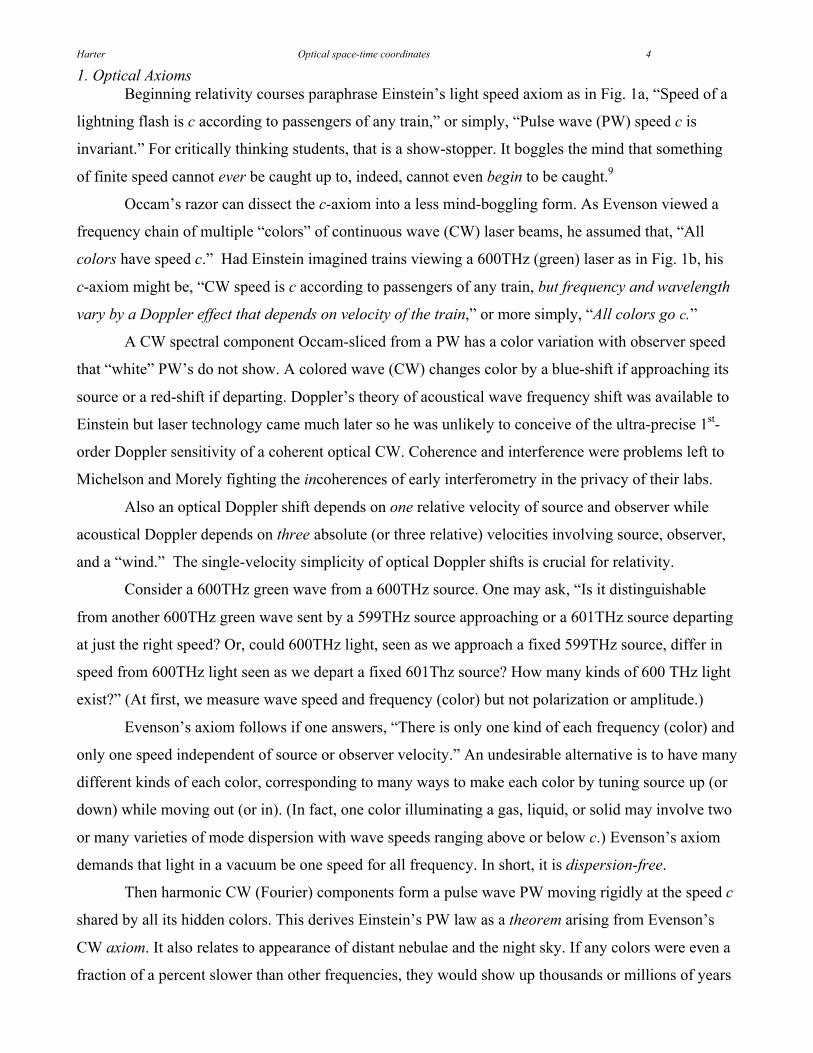
1. Optical Axioms
Beginning relativity courses paraphrase Einstein’s light speed axiom as in Fig. 1a, “Speed of a
lightning flash is c according to passengers of any train,” or simply, “Pulse wave (PW) speed c is
invariant.” For critically thinking students, that is a show-stopper. It boggles the mind that something
of finite speed cannot ever be caught up to, indeed, cannot even begin to be caught.9
Occam’s razor can dissect the c-axiom into a less mind-boggling form. As Evenson viewed a
frequency chain of multiple “colors” of continuous wave (CW) laser beams, he assumed that, “All
colors have speed c.” Had Einstein imagined trains viewing a 600THz (green) laser as in Fig. 1b, his
c-axiom might be, “CW speed is c according to passengers of any train, but frequency and wavelength
vary by a Doppler effect that depends on velocity of the train,” or more simply, “All colors go c.”
A CW spectral component Occam-sliced from a PW has a color variation with observer speed
that “white” PW’s do not show. A colored wave (CW) changes color by a blue-shift if approaching its
source or a red-shift if departing. Doppler’s theory of acoustical wave frequency shift was available to
Einstein but laser technology came much later so he was unlikely to conceive of the ultra-precise 1st-
order Doppler sensitivity of a coherent optical CW. Coherence and interference were problems left to
Michelson and Morely fighting the incoherences of early interferometry in the privacy of their labs.
Also an optical Doppler shift depends on one relative velocity of source and observer while
acoustical Doppler depends on three absolute (or three relative) velocities involving source, observer,
and a “wind.” The single-velocity simplicity of optical Doppler shifts is crucial for relativity.
Consider a 600THz green wave from a 600THz source. One may ask, “Is it distinguishable
from another 600THz green wave sent by a 599THz source approaching or a 601THz source departing
at just the right speed? Or, could 600THz light, seen as we approach a fixed 599THz source, differ in
speed from 600THz light seen as we depart a fixed 601Thz source? How many kinds of 600 THz light
exist?” (At first, we measure wave speed and frequency (color) but not polarization or amplitude.)
Evenson’s axiom follows if one answers, “There is only one kind of each frequency (color) and
only one speed independent of source or observer velocity.” An undesirable alternative is to have many
different kinds of each color, corresponding to many ways to make each color by tuning source up (or
down) while moving out (or in). (In fact, one color illuminating a gas, liquid, or solid may involve two
or many varieties of mode dispersion with wave speeds ranging above or below c.) Evenson’s axiom
demands that light in a vacuum be one speed for all frequency. In short, it is dispersion-free.
Then harmonic CW (Fourier) components form a pulse wave PW moving rigidly at the speed c
shared by all its hidden colors. This derives Einstein’s PW law as a theorem arising from Evenson’s
CW axiom. It also relates to appearance of distant nebulae and the night sky. If any colors were even a
fraction of a percent slower than other frequencies, they would show up thousands or millions of years

Harter Optical space-time coordinates 5
later with less evolved images than neighboring colors. We might then enjoy a sky full of colorful
streaks but would not have the clarity of modern astronomical images.
Spectroscopic view of CW axiom
Astronomy is just one dependent of Evenson’s CW axiom. Spectroscopy is another. Laser
atomic spectra are listed by frequency (s-1
) or period =1/ (s) while earlier tables list atomic lines
from gratings by wavenumber (m-1
) or wavelength =1/ (m). The equivalence of temporal and
spatial listings is a tacit assumption of Evenson’s axiom and may be stated as follows.
c = · = / = / = 1/( · ) = const. (1.1)
An atomic resonance is temporal and demands a precise frequency. Sub-nanometer atomic radii
are thousands of times smaller than micron-sized wavelengths of optical transitions. Optical wave-
length then seems irrelevant. (In dipole approximations, light has no spatial dependence.)
However, optical grating diffraction demands precise spatial fit of micron-sized wavelength to
micron grating slits. Optical frequency then seems irrelevant. (Bragg or Fraunhofer laws assume no
time dependence.) Spatial geometry of a spectrometer grating, cavity, or lattice directly determines a
wavelength . Frequency is determined indirectly from by (1.1). That is valid only to the extent
that light speed c = · is invariant throughout the spectrum (and throughout the universe.)
So spectroscopists expect an atomic laser cavity resonating at a certain atomic spectral line in
one rest frame to do so in all rest frames. Each or value is a proper quantity to be stamped on the
device and officially tabulated for its atoms. Passersby disagree that device output is but instead see
a Doppler red shifted r or blue shifted b . Yet, all can agree on whether the device is working!
Moreover, Evenson’s CW axiom demands that and must Doppler shift inversely one to the
other so that the product · is always a constant c=299,792,458 m·s-1
. The same applies to and
for which · =1/c. Another inverse relation exists between Doppler blue and red shifts seen before
and after passing a source. This is a CW property or axiom involving time reversal.
Time reversal axiom
Atoms behave like tiny radio transmitters, or just as well, like receivers. Unlike macroscopic
radios, atoms are time-reversible in detail since they have no resistors or similarly irreversible parts.
Suppose an atom A broadcasting frequency A resonates an approaching atom B tuned to receive a blue
shifted frequency B = b A. If time runs backwards all velocity values change sign. Atom B becomes a
transmitter of its tuned frequency B = b A that is departing from atom A who is a receiver tuned to its
frequency A = (1/b) B. Atom A sees A red-shifted from B’s frequency B by an inverse factor r=1/b.
b=1/r (1.2)
Harter Optical space-time coordinates 6
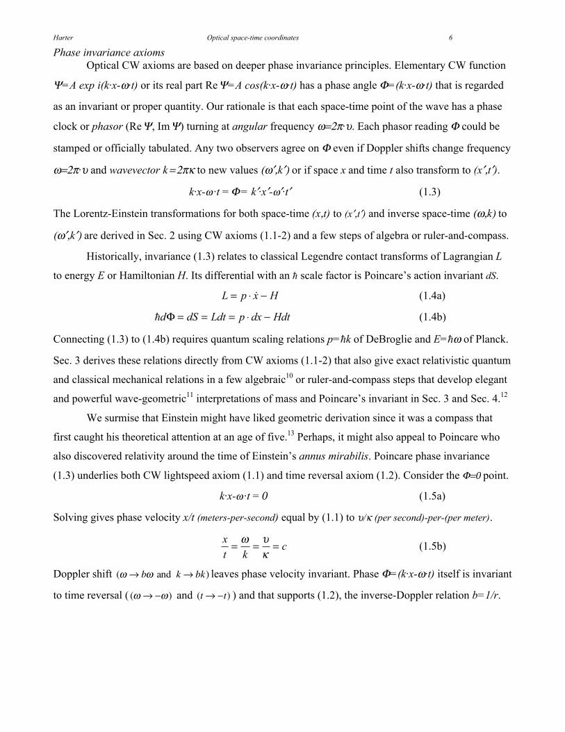
Phase invariance axioms
Optical CW axioms are based on deeper phase invariance principles. Elementary CW function
=A exp i(k·x- ·t) or its real part Re =A cos(k·x- ·t) has a phase angle =(k·x- ·t) that is regarded
as an invariant or proper quantity. Our rationale is that each space-time point of the wave has a phase
clock or phasor (Re , Im ) turning at angular frequency =2 · . Each phasor reading could be
stamped or officially tabulated. Any two observers agree on even if Doppler shifts change frequency
=2 · and wavevector k = 2 to new values ( ,k ) or if space x and time t also transform to (x ,t ).
k·x- ·t = = k ·x - ·t (1.3)
The Lorentz-Einstein transformations for both space-time (x,t) to (x ,t ) and inverse space-time ( ,k) to
( ,k ) are derived in Sec. 2 using CW axioms (1.1-2) and a few steps of algebra or ruler-and-compass.
Historically, invariance (1.3) relates to classical Legendre contact transforms of Lagrangian L
to energy E or Hamiltonian H. Its differential with an scale factor is Poincare’s action invariant dS.
L = p x H (1.4a)
d = dS = Ldt = p dx Hdt (1.4b)
Connecting (1.3) to (1.4b) requires quantum scaling relations p= k of DeBroglie and E= of Planck.
Sec. 3 derives these relations directly from CW axioms (1.1-2) that also give exact relativistic quantum
and classical mechanical relations in a few algebraic10
or ruler-and-compass steps that develop elegant
and powerful wave-geometric11
interpretations of mass and Poincare’s invariant in Sec. 3 and Sec. 4.12
We surmise that Einstein might have liked geometric derivation since it was a compass that
first caught his theoretical attention at an age of five.13
Perhaps, it might also appeal to Poincare who
also discovered relativity around the time of Einstein’s annus mirabilis. Poincare phase invariance
(1.3) underlies both CW lightspeed axiom (1.1) and time reversal axiom (1.2). Consider the =0 point.
k·x- ·t = 0 (1.5a)
Solving gives phase velocity x/t (meters-per-second) equal by (1.1) to / (per second)-per-(per meter).
x
t=
k= = c (1.5b)
Doppler shift ( b and k bk) leaves phase velocity invariant. Phase =(k·x- ·t) itself is invariant
to time reversal ( ( ) and (t t) ) and that supports (1.2), the inverse-Doppler relation b=1/r.
Harter Optical space-time coordinates 7
��� ��� ������
���
���
����� ��! ��" ��� ��� ���
��������
��������
��������
��������
��������
��������
��������
��� ���
���!���!
���"���"
��������
��������
(a)Pulse Wave (PW) #$��%��� |Ψ| &�$��'$� ReΨ�($���'$� ImΨ
(b) CW components
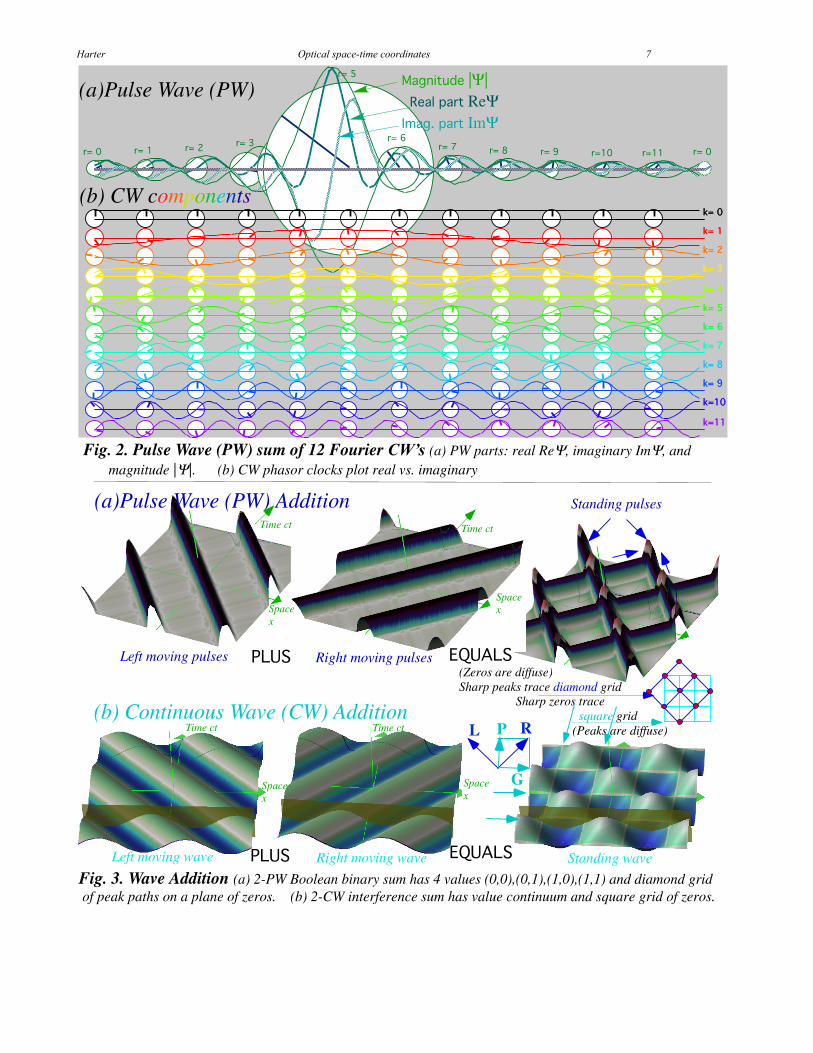
Fig. 2. Pulse Wave (PW) sum of 12 Fourier (a) PW parts: real ReΨ, imaginary ImΨ, and magnitude |Ψ|. (b) CW phasor clocks plot real vs. imaginary
)*+, -.+/*,(Zeros are diffuse)Sharp peaks trace diamond grid
(a)Pulse Wave (PW) Addition
)*+, -.+/*,
Sharp zeros trace square grid (Peaks are diffuse)
(b) Continuous Wave (CW) AdditionL R
G
P
Time ct
Spacex
Left moving pulses Right moving pulses
Standing pulses
Left moving wave Right moving wave Standing wave
Spacex
Time ct
Time ct Time ct
Spacex
Spacex
Fig. 3. Wave Addition (a) 2-PW Boolean binary sum has 4 values (0,0),(0,1),(1,0),(1,1) and diamond grid of peak paths on a plane of zeros. (b) 2-CW interference sum has value continuum and square grid of zeros.

Harter Optical space-time coordinates 8
Comparing pulsed and continuous wave trains
It is instructive to contrast two opposite wave archetypes, the Pulse Wave (PW) train sketched
in Fig. 1a and the Continuous Wave (CW) train sketched in Fig. 1b. The claim is made that the CW is
the more elementary theoretical entity, indeed the most elementary entity in classical optics since it has
just one value of angular frequency =2 · , one value of wavevector k = 2 , and one amplitude A.
CW
k , x,t( ) = Aei(kx t)
= k, x,t (1.6)
The real part is the cosine wave Acos(kx t) shown in Fig. 1(b). Acronym CW fits cosine wave, as
well. If frequency is in the visible 400-750THz range CW could also stand for colored wave.
In contrast, the PW is a less elementary wavefunction and contains N harmonic terms of CW
functions where bandwidth N is as large as possible. Fig. 2 shows an example with N=12.
PW
N (k , ) x,t( ) = A 1+ ei(kx t)
+ ei2(kx t)
+ ei3(kx t)
+ eiN (kx t)( ) (1.7)
An infinite-N PW is a train of Dirac (x-a)-functions each separated by fundamental wavelength
=2 /k. The -spikes march in lockstep at light speed c= /k following Evenson’s CW axiom.
PW
N (k , ) x,t( )N
A x ct n( )n=
Delta functions have infinite frequency bandwidth and are thus impractical. Realistic PW trains apply
cutoff or tapering amplitudes an to each harmonic to restrict frequency to a finite bandwidth .
PWx,t( ) = a
ne
in(kx t)
n=0= G x ct n( )
n=
where: an
1 for n > (1.8)
A common choice is a Gaussian taper an = en /( )
2
that gives Gaussian PW functions G( ) = e ( )2
.
PW functions (1.8) involve an unlimited number of amplitude parameters an in addition to
fundamental frequency , while a CW function has a single amplitude parameter A. Thus, theory based
on CW properties would seem to be closer to an Occam ideal of simplicity than one based on PW.
However, with regard to counter-propagating or colliding beams the PW appear in Fig. 3a to
have simpler properties than CW in Fig. 3b. PW have a simple classical Boolean OFF (0) over most of
space-time with an occasional ON (1) at a sharp pulse. On the other hand CW range gradually between
+1 and –1 over most of space-time, but have a sharp zero (0) in between crest and trough. (A PW can
be designed to show precisely where it is. A CW naturally shows precisely where it is not.)
Interference of colliding PW is wysiwye (What you see is what you expect.), but the pattern of
interference for the sum of colliding CW is subtler. PW paths in space-time (x,ct) resemble baseball
diamonds like the baseline paths in the American sport, while the CW zeros are Cartesian space-time

Harter Optical space-time coordinates 9
squares made of horizontal spatial x-axial lines of equal times (ct=…1,2…) and vertical temporal ct-
axial lines of fixed location (x=…1,2…). PW diamonds, while deceptively simple, cover up a
complicated network of zeros around each pulse. CW squares are a simple lattice of zeros for a
standing wave that is just a factored sum of the following two equal-but-opposite colliding CW.
CWk , +
CWk , = A ei(kx t)
+ ei( kx t)( ) = 2Ae i t cos(kx)( ) (1.9)
The group envelope factor cos(kx)( ) is zero along ct-axial lines of position (kx/ +1/2=…0,1,2…). The
phase factor (e i t ) has zero real part along x-axial lines of simultaneous time (ct/ +1/2=…0,1,2…).
Comparing wave-zero (WZ) and pulse-peak (PP) coordinates
It is now shown how general phase and group wave zeros of 2-CW interference define a space-
time wave-zero (WZ) coordinate grid that complements a pulse peak or particle-path (PP) grid of 2-
PW trains. This helps to visualize the wave-particle duality whose history goes back to Newton’s
corpuscular view of light before wave optics of Maxwell-Young or after Planck-Einstein physics of
quanta. The visualization is done by superimposing a time-vs-space (x,t)-plot on top of its Fourier
inverse per-time-space or reciprocal space-time plot of frequency-vs-wavevector ( ,k).
The plots apply to general wave mechanics and not just optics. An example in Fig. 4 begins by
picking four random numbers, say, 1,2,4, and 4 to insert into frequency-wavevector K2= ( 2,k2)=(1,2)
of a mythical source-2 and frequency-wavevector K4= ( 4,k4)=(4,4) of another mythical source-4.
(This is not light. Slope or velocity c2= 2 /k2 =1/2 of source-2 differs from c4= 4 /k4 =1 of source-4.)
Let continuous waves (CW) from the two sources interfere in a 2-CW sum.
2 CW= (e
i k4 x 4t( )+ e
i k2 x 2t( )) / 2 (1.10a)
To solve for zeros of this sum we first factor it into a phase-wave eip and a group-wave cos g factor.
2 CW= e
ik4 +k2
2x 4 + 2
2t
(ei
k4 k2
2x 4 2
2t
+ ei
k4 k2
2x 4 2
2t
) / 2
= ei
k4 +k2
2x 4 + 2
2t
cosk
4k
2
2x 4 2
2t
= ei kp x pt( ) cos kgx gt ( ) eip cos g
(1.10b))
Phase factor eip
has a half-sum ( ,k)-vector Kphase=(K4+K2)/2 in its argument p = kpx pt . Group
factor cos g has a half-difference ( ,k)-vector Kgroup=(K4 K2)/2 in its argument g = kgx gt .
K phase =K4 + K2
2=
1
24 + 2
k4 + k2
=p
kp
=1
2
4 +1
4 + 2=
2.5
3.0
(1.10c)
Kgroup =K4 K2
2=
1
24 2
k4 k2
=g
kg
=1
2
4 1
4 2=
1.5
1.0
(1.10d)

Harter Optical space-time coordinates 10
K4
K2
Wave group vectors
Frequency ω
Wave phase zero-paths
Kphase=(2.5, 3.0)
Kphase
Kgroup=(1.5, 1.0)
K4K2Kgroup
Space x
Kgroup=(K4-K2)/2
Wavevector kTime t
(b)Per-spacetime (ω,k)
Wavegroupnode-paths
Wave phase vectors
(a) Spacetime (x,t)
Kphase=(K4+K2)/2
PWlattice
CWlattice
source 2
source 4
K2=(ω2,k2)
=(1, 2)
K4=(ω4,k4)
=(4, 4)
Fig. 4 “Mythical” sources and their wave coordinate lattices in (a) Spacetime and (b) Per-spacetime.
CW lattices of phase-zero and group-node paths intermesh with PW lattices of pulse, packet, or “particle” paths.

Harter Optical space-time coordinates 11
The ( ,k)-vectors Kn define paths and coordinate lattices for pulse peaks and wave zeros in Fig. 4a.
Real zeros (Re =0) have speed Vphase on Kphase paths. Group zeros (| |=0) move at Vgroup on Kgroup.
Vphase =4 + 2
k4 + k2
=5
6= 0.83 (1.11a) Vgroup =
4 2
k4 k2
=3
2= 1.5 (1.11b)
Phase factor real part Re eip= Re e
i kpx pt( )= cos p zeros on phase-zero paths where angle p is N(odd)· /2.
kpx pt = p = N p / 2 N p = ±1,±3...( ) .
Group factor cos g = cos kgx
gt( ) zeros on group-zero or nodal paths where angle g is N(odd)· /2.
kgx gt = g = Ng / 2 Ng = ±1,±3...( ) .
At wave zero (WZ) lattice points (x,t) both factors are zero. That defines the lattice vectors in Fig. 4a.
kp p
kg g
x
t=
p
g=
N p
Ng 2 (1.12a)
Solving gives spacetime (x,t) zero-path lattice shown by the white lines in Fig. 4a. Each intersecting
lattice point is an odd-integer (Np, N
g) combination of wave-vectors P = K
phase/ 2D and G = K
group/ 2D .
x
t=
g p
kg kp
p
g
pkg gkp
=
-pg
kg
+gp
kp
pkg gkp
=2D
( N pKgroup+NgK phase ) (1.12b)
Scaling factor 2D/ = 2( pkg gkp) / converts (per-time, per-space) vectors Kgroup or Kphase into
(space, time) vectors P = (tx )
por G = (
tx )
g. (Plot units are set so 2D/ =1 or D= /2 iff D is non-zero.)
Fig. 4b is a lattice of source vectors K2 and K4 (the difference and sum of Kgroup and Kphase).
K2 = K phase Kgroup =2
k2
=1
2(1.13a) K4 = K phase +Kgroup =
4
k4
=4
4(1.13b)
Phase of source-2 has speed V2 on K2 paths. Phase of source-4 has speed V4 on K4 paths.
V2 =2
k2
=1
2= 0.5 (1.14a) V4 =
4
k4
=1
1= 1.0 (1.14b)
However, one can view the K2 and K4 paths in light of a classical or semi-classical viewpoint since
pulse waves (PW) are wave packets (WP) that mimic particles. Newton took a hard-line view of nature
and ascribed reality to mass particles but viewed waves as illusory. He misunderstood light when it
exhibited interference effects and complained that its particles or “corpuscles” were having “fits.”
Newtonian corpuscular views are parodied here by imagining that frequency 2 = 2 / 2
(or 4 = 4 / 2 ) is the rate at which source-2 (or 4) emits “corpuscles” of velocity V2 (or V4) so the
wavelengths 2 = 2 / k2 (or 4 = 2 / k4 ) are just inter-particle spacing of K2 (or K4) lines in Fig. 4a.

Harter Optical space-time coordinates 12
Since wavelength 2 ( 4 ) separates K2 (K4 ) lattice lines in Fig. 4b, one can imagine them as “corpuscle
paths” on diagonals of the Kgroup(Kphase) WZ-lattice in time vs space (x,t) of Fig. 4a.
Left and right baseline vectors L and R of diamonds in Fig. 3a are special cases of K2 and K4
vectors (1.13). Diamond paths in Fig. 3a are ±45° pulse wave (PW) paths due to a multi-term CW sum
(1.17). Still, one might imagine pulses are “corpuscles” or particles, and the L(-45°) and R(+45°) paths,
like the K2 and K4 “corpuscle” paths in Fig. 4b, are baselines for some kind of “optical base runners.”
The square wave zero (WZ) grid in Fig. 3b is due to a two-term CW sum (1.9). It is a special
case of the WZ lattice in Fig. 4a due to two-term sum (1.10). Half-sum phase vector P = (L + R) / 2 and
half-difference group vector G = (L R) / 2 define a square grid of nodal lines in Fig. 3a. Vectors P and
G are a square example of the phase and group lattice vectors Kphase and Kgroup in (1.10) that define a
non-square WZ path lattice of white lines (real zeros) in Fig. 4a. (Sec.2 analyzes Fig. 3 in detail.)
Primitive vectors L and R are optical pulse wave (PW) or particle paths (PP) in Fig. 3a while in
Fig. 3b their half-sum P = (L + R) / 2 and half-difference G = (L R) / 2 define optical phase and group
wave zero (WZ) coordinate grid lines. Phase and group WZ lines are time and space axes, respectively,
forming an optical coordinate basis for our subsequent development of relativistic quantum mechanics.
This development shows wave-particle, wave-pulse, and CW-PW duality in the cells of each
CW-PW wave lattice. Each (L,R)-cell of a PW lattice has two CW vectors P or G on each diagonal,
and each (P,G)-cell of the CW lattice has one PW vector L or R on each diagonal. This is due to sum
and difference relations (1.10d) or (1.13b) between (L,R)= (K2, K4) and (P,G)=(Kphase, Kgroup).
In order that space-time (x,t)-plots could be superimposed on frequency-wavevector ( ,k)-plots
or ( , )-plots, it is necessary to switch axes for one of them. The space-time t(x)-plots in Fig. 4a follow
the convention adopted by most relativity literature for a vertical time ordinate (t-axis) and horizontal
space abscissa (x-axis) that is quite the opposite of Newtonian calculus texts that plot x(t) horizontally.
However, the frequency-wavevector k( )-plots in Fig. 4b switch axes from the usual (k) convention
so that t(x) slope due to space-time velocity x/t or x/ t (meter/second) in Fig. 4a matches that of equal
per-time-per-space wave velocity /k or / k (per-second/per-meter) in Fig.4b. (Recall (1.5))
Superimposing t(x)-plots onto k( )-plots also requires that the latter be rescaled by the scale
factor /2D derived in (1.12b), but rescaling fails if cell-area determinant factor D is zero.
D = pkg gkp = K phase Kgroup (1.15)
Co-propagating light beams K2= ( 2,k2)=(2c,2) and K4= ( 4,k4)=(4c,4) plotted in Fig. 5b have D=0 since
all K-vectors including Kphase=( p,kp)=(3c,3) and Kgroup= ( g,kg)=(c,1) lie on one c-baseline of speed c
that has unit slope ( /ck=1). We rescale ( ,k)-plots to ( ,ck) and (x,t)-plots to (x,ct) in Fig. 5 and later.

Harter Optical space-time coordinates 13
K4
K2Kphase=(K4+K2)/2
Wav
evec
tor
ck κ
Frequency ω
Wave zero-paths all the same speed c
(a) Spacetime (x,ct) (b) Per-spacetime (ω,ck)
Space x
Tim
e ct
Kgroup=(K4-K2)/2
Infrared laser
Krypton laser
source 2
source 4
K2=(ω2,k2)
=(2c, 2)
K4=(ω4,k4)
=(4c, 4)
Replaced by:
Fig. 5 Co-propagating laser beams produce a collapsed wave lattice since all parts have same speed c.
For counter propagating waves shown in Fig. 3 and Fig. 6-7 below, D is not zero because two
opposite (right-left) baselines (R,L)= (K2, K4) are used to make CW square bases (P= Kphase, G= Kgroup)
with a non-zero value for area D =|GxP|, an axis-switch of (1.15). PW base vectors (R,L) are sum and
difference (P+G,P-G) of CW bases so a PW diamond area |RxL| is twice that of a CW square.
|RxL|= |(P+G) x (P-G)| =2|GxP| (1.16)
It will be shown that these areas are key geometric invariants for relativity and quantum mechanics.

Harter Optical space-time coordinates 14
2.Wave coordinates for counter-propagating beams
Let us represent counter-propagating frequency- laser beams by a baseball diamond in Fig. 6a
spanned by CW vectors for waves moving left-to-right (R on 1st base) and right-to-left (L on 3
rd base).
R=K1=(ck1, 1)= (1,1) (2.1a) L=K3=(ck3, 3)= (-1,1) (2.1b)
Fig. 6 uses conventional (ck, )-plots for per-space-time and (x,ct)-plots for space-time. Both beams
have frequency = /2 =600THz(green), the unit scale for and ck axes. For the L-beam, ck is - .
Phase vector P=Kphase and group vector G=Kgroup are also plotted in ( ,ck)-space in Fig. 6b.
K phase =K1 + K3
2=
1
2
ck1 + ck3
1 + 3
= P =
ckp
p
=2
1 1
1+1=
0
1
(2.2a)
Kgroup =K1 K3
2=
1
2
ck1 ck3
1 3
= G =
ckg
g
=2
1+1
1 1=
1
0
(2.2b)
Phase and group velocities of counter-propagating light waves may vary widely from c. These do!
Vphase
c=
1 + 3
ck1 + ck3
=2
0= (2.3a)
Vgroup
c=
1 3
ck1 ck3
=0
2c= 0 (2.3b)
The extreme speeds account for the square (Cartesian) wave-zero (WZ) coordinates plotted in Fig. 6c.
As noted after Fig. 3, the group zeros or wave nodes are stationary and parallel to the time ct-axes,
while the real-zeros of the phase wave are parallel to the space x-axes. The latter instantly appear and
disappear periodically with infinite speed (2.3a) while standing wave nodes have zero speed (2.3b).
Fig. 6d shows 2-way pulse wave (2-PW) trains for comparison with the 2-CW WZ grid in Fig.
6c. As noted after Fig. 2, a PW function is an N-CW combination that suppresses its amplitude through
destructive interference between pulse peaks that owe their enhancement to constructive interference.
Colliding PW’s show no mutual interference in destroyed regions. Generally one PW is alone
on its diamond path going +c parallel to 1st baseline R=K1 or going –c parallel to 3
rd baseline L=K3.
V1
c=
1
ck1
=1
1= 1 (2.4a)
V3
c=
3
ck3
=1
1= 1 (2.4b)
But wherever two PW peaks collide, each of the CW pairs will be seen trying to form a square
coordinate grid that 2-CW zeros would make by themselves. This begins to explain the tiny square
“bases” seen at the corners of the space-time “baseball diamonds” in Fig. 6d.
CW-Doppler derivation of relativity
Occam razors shorten derivations. How much does Evenson’s CW razor-cut of Einstein’s PW
axiom shorten derivation of relativity? Quantifying length for Einstein’s popular (and still common)
derivation is difficult as is a step-by-step count for the CW derivation that follows. Let us just say that
several steps are reduced to very few steps. More important is the wave-nature insight that is gained.

Harter Optical space-time coordinates 15
K pK 3K 1
K g
ck
ω
2ω
ω
(b) Laser group and phase wavevectors (Per-space-time Cartesian lattice)
L=K 3 R=K 1
per-timeω=2π ν
ω
2ω
� per-spaceck=2πc κ
space x
time ct Abs|Ψ|
Re Ψ Im Ψ
(c) Laser Coherent Wave (CW) paths (Space-time Cartesian grid)
(d) Laser Pulse Wave (PW) Paths (Space-time Diamond grid)
space x
time ct
P
O
1st base
2nd base
3rd base
600Thz
Left-to-RightBeam
600Thz
Right-to-LeftBeam
λ = 1 μm2 4
0
1ω
1
0ω
Fig. 6. Laser lab view of 600Thz CW and PW light waves in per-space-time (a-b) and space-time (c-d).
In fact, a case can be made that a CW derivation takes zero steps. The answer is already done
by a 2-CW wave pattern in Fig. 7c that automatically produces an Einstein-Lorentz-Minkowski14
grid
of space-time coordinates. Still we need logical steps drawn in Fig. 7a-b that redo the Cartesian grid in
Fig. 6 just by Doppler shifting each baseline one octave according to c-axiom (1.1) (“Stay on baselines!”)
and t-reversal axiom (1.2) (“If 1st base increases by one octave, 3
rd base decreases by the same.”)

Harter Optical space-time coordinates 16
So Fig. 7 is just Fig. 6 seen by atoms going right-to-left fast enough to double both frequency
= /2 and wavevector ck of the vector R on 1st base (while halving vector L on 3
rd base to obey (1.2).)
R=K1=( ck 1, 1)= (2,2) (2.5a) L=K3=( ck 3, 3 )= (-1/2, 1/2) (2.5b)
The atom sees head-on R-beam blue-shift to frequency 1 =2 = 1 /2 =1200THz(UV) by doubling green
1= /2 = 3=600THz. It also sees the tail-on L-beam red-shift by half to 3 = /2= 3 /2 =300THz(IR).
The phase vector Kphase and group vector Kgroup are plotted in (ck , )-space in Fig. 7b.
K phase =K1 + K3
2=
1
2
ck1 + ck3
1 + 3
= P =
ckp
p
=2
2 1 / 2
2 +1 / 2=
3 / 4
5 / 4
(2.6a)
Kgroup =K1 K3
2=
1
2
ck1 ck3
1 3
= G =
ckg
g
=2
2 +1 / 2
2 1 / 2=
5 / 4
3 / 4
(2.6b)
Phase velocity is the inverse of group velocity in units of c, and V group is minus the atoms’ velocity!
Vphase
c=
1 + 3
ck1 + ck3
=2 +1 / 2
2 1 / 2=
5
3(2.7a)
Vgroup
c=
1 3
ck1 ck3
=2 1 / 2
2 +1 / 2=
3
5(2.7b)
Velocity u=V group =3c/5 is the atoms’ view for a lab speed of zero had by laser standing nodes. (It is the
speed of the lasers’ group nodes and their connecting lab bench relative to the atoms.) Phase velocity
V phase =5c/3 is the atoms’ view for a lab speed of infinity had by lasers’ real wave zeros. (x-zero lines
are simultaneous in the laser lab but not so in the atom-frame. x-lines tip toward ct-lines in Fig. 7c.)
Eqs. (2.5-7) use a Doppler blue-shift factor b=2. If each “2” is replaced by “b” then Eq. (2.7b)
yields a relation for the laser velocity u=V group relative to atoms in terms of their blue-shift b.
Vgroup
c=
u
c=
b 1 / b
b +1 / b=
b2 1
b2+1
(2.8a)
Inverting this gives standard relativistic Doppler b vs. u/c relations.
b2= 1+ u / c( ) / 1 u / c( ) or: b = 1+ u / c( ) / 1 u / c( ) = 1+ u / c( ) / 1 u2 / c2 (2.8b)
It is remarkable that most treatments of relativity first derive second order effects, time dilation and
length contraction. Doppler and asimultaneity shifts are first order in u but treated second. Setting 2=b
in (2.6) using (2.8) gives vectors G = Kg = (ad ) and P = K p = (d
a ) with dilation factor d = 1 / 1 u2 / c2
and asimultaneity factor a=u·d/c. (So d arrives early here, too, but with a wavelike finesse.)
K phase =2
b 1 / b
b +1 / b=
(u / c) / 1 u2 / c2
1 / 1 u2 / c2(2.9a) Kgroup =
2
b +1 / b
b 1 / b=
1 / 1 u2 / c2
(u / c) / 1 u2 / c2(2.9b)
K-vector components d and a (in units) are Lorentz-Einstein (LE) matrix coefficients relating atom-
values (ck , ) or (x ,t ) to lab-values (ck, ) or (x,t) based on lab unit vectors G = 01( ) and P = 1
0( ) in (2.2).
Harter Optical space-time coordinates 17
ck
(b) Boosted group and phase wavevectors (Per-space-time Minkowski lattice)
L=K 3 R=K
1
(Per-space-time rectangle)
per-time=2π ν
per-space
ck =2πc κ
ω
2ω
�
R=K 1
L =K 3
ω
2ω
�
K 1
K 3
ω
(c) (u=3c/5)-Boosted CW paths (Space-time Minkowski grid)
space x
timect
time ct
space x
spacex
timect
(d) Boosted PW Paths (Rectangular grid)
ωckg
ω g
= 45
43
ω
ck p
ω p
= 43
45
ω
1200Thz
Left-to-RightBeam
300Thz
Right-to-LeftBeam
k Rk L
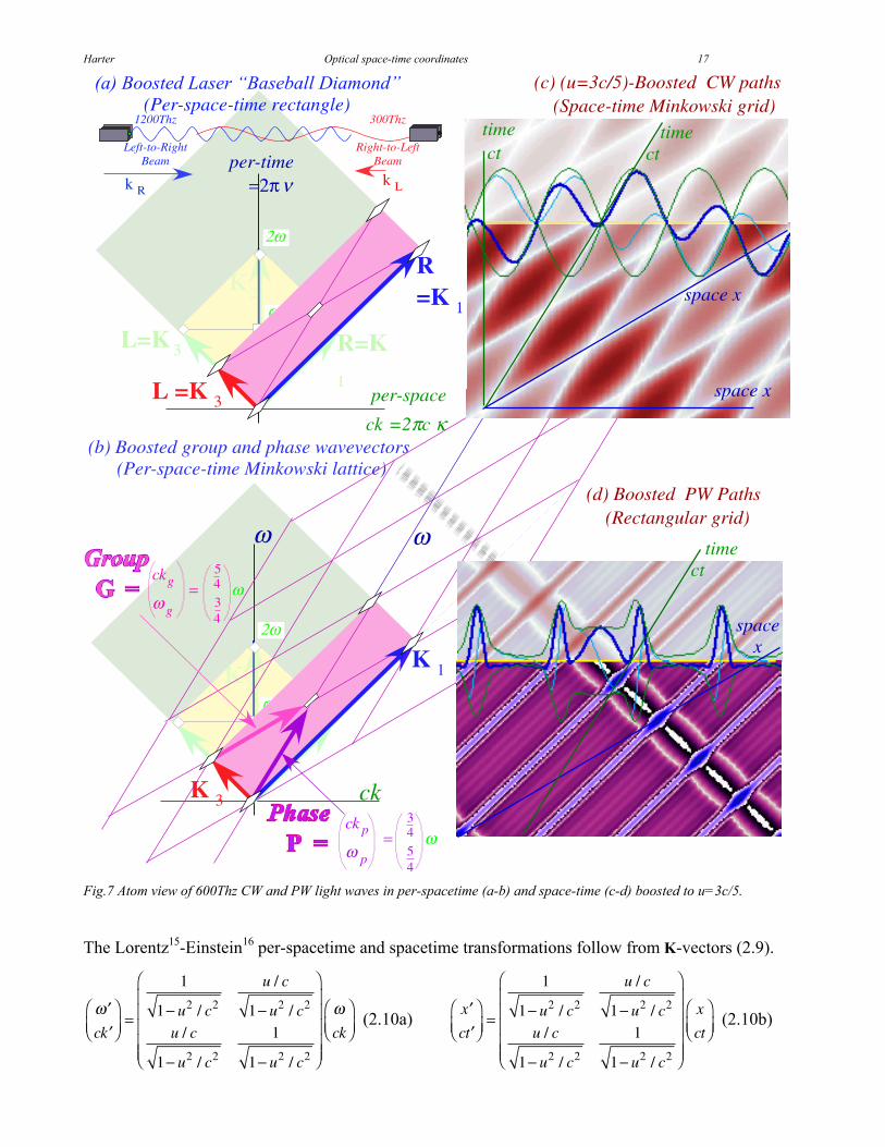
Fig.7 Atom view of 600Thz CW and PW light waves in per-spacetime (a-b) and space-time (c-d) boosted to u=3c/5.
The Lorentz15
-Einstein16
per-spacetime and spacetime transformations follow from K-vectors (2.9).
ck=
1
1 u2 / c2
u / c
1 u2 / c2
u / c
1 u2 / c2
1
1 u2 / c2
ck (2.10a)
x
ct=
1
1 u2 / c2
u / c
1 u2 / c2
u / c
1 u2 / c2
1
1 u2 / c2
x
ct (2.10b)

Harter Optical space-time coordinates 18
Wave K-vectors are bases for space-time and per-space-time. One symmetric LE matrix, invariant to
axis-switch ( ,ck)
(ck, ), applies to both. Conventional ordinate vs. ck-abscissa per-space-time and
ct-ordinate vs. x-abscissa space-time plots are used in Fig. 7 where =P=Kphase and
ck =G=Kgroup vectors
serve as ct-time and x-space bases, respectively, and then also serve as and-ck-bases.
The left and right pulse wave (PW) vectors L and R in per-space-time Fig. 7a also define left
and right PW paths in space-time Fig. 7d. This holds in either convention because L and R lie on 45°
reflection planes that are eigenvectors of an axis-switch ( ,ck)
(ck, ) with eigenvalues +1 and –1
while half-sum-and-difference vectors P = (L + R) / 2 and G = (L R) / 2 simply switch (P
G).
Einstein’s PW axiom “PW speed c is invariant,” might give the impression that pulses themselves
are invariant. This may hold for -pulses whose infinite bandwidth gives them enough energy to start a
new universe! But, finite- pulses in Fig. 7d clearly deform. Only their speed is invariant. Also, each
PW intersection-interference square in Fig. 6d deforms into a Minkowski-like rhombus in Fig. 7d.
Geometry of relative phase
Einstein relativity shows Galilean relativity, based on simple velocity sums and differences, to
be a 400 year-old approximation that fails utterly at high speeds. Einstein also dethrones infinite
velocity, Galileo’s one invariant velocity shared by his observers regardless of their (finite) velocity. In
its place reigns a finite velocity limit c that is now the Einstein-Maxwell-Evenson invariant.
So it is remarkable that frequency sums and differences (1.10) simplify relativity by using
Galilean-like rules for angular velocities A = A of light phases A . Frequency sums or differences
A ± B from interference terms like A B* = ABe i( A B )tbetween wave pairs A = Ae i At
and
B = Be i Bt are relative frequencies (beat notes, overtones, etc.) subject only to simple addition and
subtraction rules that are like Galileo’s rules for linear velocity. Simple angular phase principles deeply
underlie modern physics, and so far there appears to be no c-like speed limit for an angular velocity .
Phase principles have electromagnetic origins. Writing oscillatory wave functions using real
and imaginary parts is common for studies of AC electrical phenomena or harmonic oscillators in
general. The real part q of oscillator amplitude q+ip= Ae i t is position q=Acos t. The imaginary part
p=Asin t is velocity v =-A sin t in units of angular frequency . Positive gives a clockwise rotation
like that of classical phase space or analog clocks, so a minus sign in conventional Ae i t phasors serves
to remind us that wave frequency defines our clocks and wavevector k= /c defines our meter sticks.
A plane wave of wavevector k in Fig. 2 is drawn as a phasor array, one A = A ei kx for each
location x. A plane wave advances in time according to A ei(kx t ) at phase velocity V= /k. Similar
Harter Optical space-time coordinates 19
convention and notation are used for light waves and for quantum matter waves, but only light waves
have physical units, vector potential A and electric E-field, defining their real and imaginary parts.
While classical laser wave phase is observable, only relative quantum wave phase appears to be so.
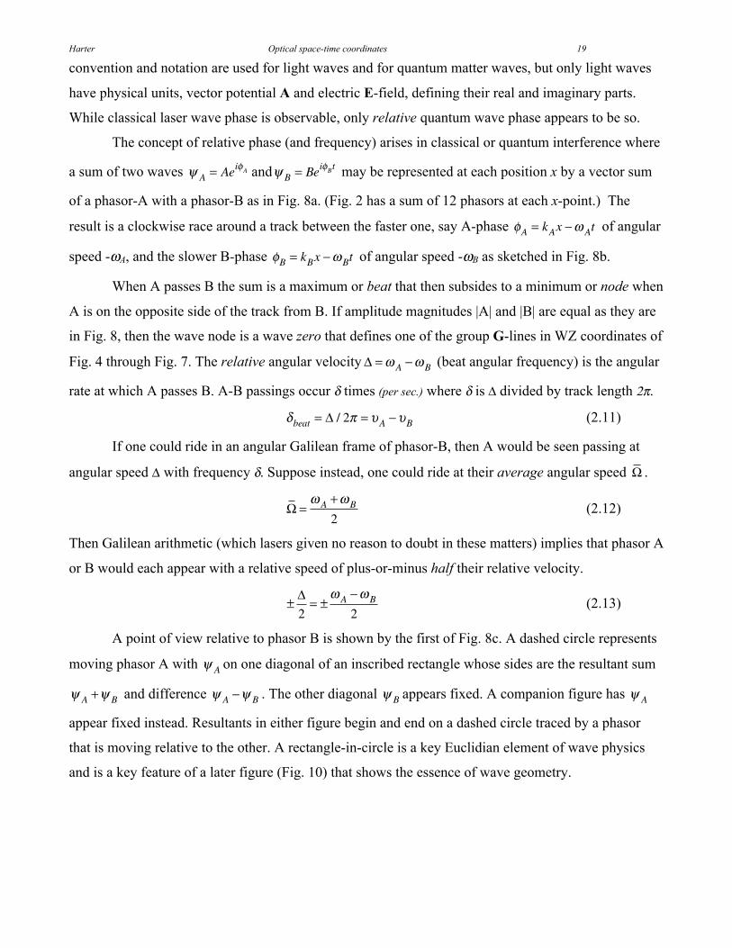
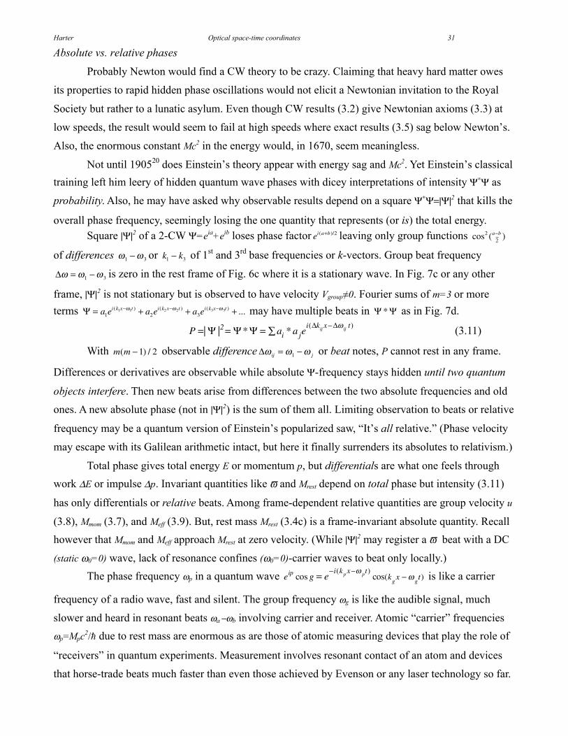
The concept of relative phase (and frequency) arises in classical or quantum interference where
a sum of two waves A = Aei A and B = Bei Bt may be represented at each position x by a vector sum
of a phasor-A with a phasor-B as in Fig. 8a. (Fig. 2 has a sum of 12 phasors at each x-point.) The
result is a clockwise race around a track between the faster one, say A-phase A = kAx At of angular
speed - A, and the slower B-phase B = kBx Bt of angular speed - B as sketched in Fig. 8b.
When A passes B the sum is a maximum or beat that then subsides to a minimum or node when
A is on the opposite side of the track from B. If amplitude magnitudes |A| and |B| are equal as they are
in Fig. 8, then the wave node is a wave zero that defines one of the group G-lines in WZ coordinates of
Fig. 4 through Fig. 7. The relative angular velocity = A B (beat angular frequency) is the angular
rate at which A passes B. A-B passings occur times (per sec.) where is divided by track length 2 .
beat = / 2 = A B (2.11)
If one could ride in an angular Galilean frame of phasor-B, then A would be seen passing at
angular speed with frequency . Suppose instead, one could ride at their average angular speed .
=A + B
2(2.12)
Then Galilean arithmetic (which lasers given no reason to doubt in these matters) implies that phasor A
or B would each appear with a relative speed of plus-or-minus half their relative velocity.
±2= ±
A B
2(2.13)
A point of view relative to phasor B is shown by the first of Fig. 8c. A dashed circle represents
moving phasor A with A on one diagonal of an inscribed rectangle whose sides are the resultant sum
A + B and difference A B . The other diagonal B appears fixed. A companion figure has A
appear fixed instead. Resultants in either figure begin and end on a dashed circle traced by a phasor
that is moving relative to the other. A rectangle-in-circle is a key Euclidian element of wave physics
and is a key feature of a later figure (Fig. 10) that shows the essence of wave geometry.

Harter Optical space-time coordinates 20
B moves relative to A
PLUS
β
αcosα
sinα
cosβ
Red phasor B
EQUALS:
Green phasor A
(α+β)/2
(α−β)/2
(α−β)/2
(b) Typical Phasor Sum:
��� ��� ��� ��� ��� ��� ��� �� ��! ��" ��� ��� ��� ��� ��� ��� ���
A moves relative to B
(c) Phasor-relative views
(a) Sum of Wave Phasor Array
A
A B
B
ψA=eiα
ψB=eiβ
Sum: ΨA+B=ψA+ψB
Difference:ΨA−B=ψA−ψB
ΨA+B=ψA+ψB
(α−β)
Fig. 8 Wave phasor addition. (a) Each phasor in a wave array is a sum (b) of two component phasors.
(c) In phasor-relative views either A or else B is fixed. An evolving sum-and-difference rectangle is inscribed in the
(dashed) circle of the phasor moving relative to the fixed one.

Harter Optical space-time coordinates 21
The half-sum and half-difference angles in Fig. 8b and frequencies (2.12) and (2.13) appear in
the interference formulas (1.10) that lead to relativistic Lorentz-Einstein coordinate relations (2.10) and
their WZ grid plots of Minkowski coordinates in Fig. 7c. One key is the arithimetic mean ( + ) / 2 of
phases that gives the geometric mean ( A B )1/2= Aei( + ) /2 of wave phasor amplitudes. The other key
is the difference mean ( ) / 2( ) and its cross mean ( A B*)1/2= Aei( ) /2 . Euclidian means and
rectangle-in-circle constructions underlie relativistic wave geometry and mechanics as is shown below.
Geometry of Doppler factors
Any number N of transmitter-receivers (“observers” or “atoms” previously introduced) may
each be assigned a positive number b11, b21, b31, …that is its Doppler shift of a standard frequency 1
broadcast by atom-1 and then received as frequency m1= bm1 1 by an atom- m. By definition the
transmitter’s own shift is unity. (1= b11) Also, coefficient bm1 is independent of frequency since such
geometric relations work as well on 1THz or 1Hz waves as both waves march in lockstep to the
receiver by Evenson’s CW axiom (1.1). The production times of a single wavelength of the 1Hz-wave
and 1012
wavelengths of the 1THz wave must be the same (1sec.), and so must be reception time for the
two waves since they arrive in lock step, even if is shortened geometrically by 1/ bm1.
If atoms travel at constant speeds on a straight superhighway, then bm1 in (2.8a) tells what is the
relative velocity um1 of the mth
atomic receiver relative to the number-1 transmitter.
um1
c=
bm12 1
bm12+1
(2.14)
The velocity um1 is positive if the mth
atom goes toward transmitter-1 and sees a blue (bm1>1) shift, but
if it moves away um1 is negative so it sees a red (bm1<1) shift. Transmitter-1 has no velocity relative to
itself. (u11=0) Infinite blue (or red) shift bm1= (or bm1=0) gives um1=c (or um1=-c) and this defines the
range of parameters. The bm1 are constant until atom-m passes atom-1 so relative velocity changes sign
( u1m u1m ). Doppler shift then inverts ( b1m 1 / b1m ) as is consistent with axiom (1.2).
Suppose now b12, b22, b32, …are Doppler shifts of frequency 2 transmitted by the second atom
and received by the mth
atom as frequency m2= bm2 2. (Any atom (say the nth
) may transmit, too.)
mn= bmn n (2.15a)
Recipients do not notice if atom-n simply passes on whatever frequency nm came from atom-m. If
frequency n in (2.15a) is n1= bn1 1 that atom-n got from atom-1 then atom-m will not distinguish a
direct m1 from a perfect copy bmn bn1 1 made by atom-n from atom-1 and then passed on to atom-m.
m1 = bm1 1= bmn bn1 1 (2.15b)

Harter Optical space-time coordinates 22
A multiplication rule results for Doppler factors and applies to light from atom-1 or any atom-p.
mp/ p= bmp = bmn bnp (2.15c)
An inverse relation results from atom-p comparing its own light to that copied by atom-n.
1= bpp = bpn bnp or: bpn =1/bnp (2.15d)
Notice that copying or passing light means just that and does not include reflection or changing
+k to –k or any other direction. This presents a problem for a receiver not in its transmitter’s (+k)-beam
and certainly for atom-p receiving its own beam. The relations (2.15) depend only on relative velocities
and not positions (apart from the problem that receivers might be on the wrong side of transmitters).
An obvious solution is to let the receiver overtake its transmitter or failing that delegate a slave
transmitter or receiver on its right side. A more elegant solution is to conduct experiments in a large
circular coaxial (dispersion-free) waveguide or ring laser so the (+k)-beam illuminates the backside as
well as forward. Fig. 9 shows one arrangement with N=5 receivers of a 3=600THz source whose
various speeds produce a matrix of N(N-1)=20 Doppler shifted frequencies mn and factors bmn.
300THz 400THz 600THz 900THz 1200THz300THz 300/300 300/400 300/600 300/900 300/1200
b11=1 b12=0.75 b13=0.5 b14=0.333 b15=0.25
400THz 400/300 400/400 400/600 400/900 400/1200b21=1.333 b22=1 b23=0.667 b24=0.449 b25=0.333
600THz 600/300 600/400 600/600 600/900 600/1200 b31=2 b32=1.5 b33=1 b34=0.667 b35=0.5
900THz 900/300 900/400 900/600 900/900 900/1200 b41=3 b42=2.25 b43=1.5 b44=1 b45=0.75
1200THz 1200/300 1200/400 1200/600 1200/900 1200/1200 b51=4 b52=3 b53=2 b54 =1.333 b55 =1
10Dopplerred-shiftratios:rl,h = υlo/υhi
10 Doppler blue-shift ratios: b h,l = υhi/υlo
5 Doppler
fixedreceiver
blue shifted oncoming receiversred shifted departing receivers
,�+&0-,�+&0-
,�+&0-,�+&0-,�+&0-
&-0-�1-&&-0-�1-&
&-0-�1-&&-0-�1-& &-0-�1-&&-0-�1-&
&-0-�1-&&-0-�1-& &-0-�1-&&-0-�1-&
&-0-�1-&&-0-�1-&&-0-�1-&&-0-�1-&
&-0-�1-&&-0-�1-& &-0-�1-&&-0-�1-&&-0-�1-&&-0-�1-&
greenreference
source
Fig. 9 Doppler shift b-matrix for a linear array of variously moving receiver-sources.

Harter Optical space-time coordinates 23
Doppler rapidity and mean values
Composition rules (2.15c) suggest defining Doppler factors b=e in terms of rapidity =ln b.
bmp = bmn bnp implies: mp = mn + np where: bab = e ab (2.16)
Rapidity parameters mn mimic Galilean addition rules as do phase angles of wavefunctionss ei , and
and are the parameters that underlie relativity and quantum theory. In fact, by (2.14) rapidity mn
approaches the relative velocity parameter umn /c between atom-m and atom-n for speeds much less
than c. Rapidity is also convenient for astronomically large Doppler ratios bab since then the numerical
value of ab =ln bab is much less than bab while the value of umn /c inconveniently approaches 1.
At intermediate relativistic speeds the geometric aspects of Doppler factors provide a simple
but precise and revealing picture of the nature of wave-based mechanics. Any pair of counter moving
continuous waves (CW) has mean values between a K-vector R=K1=(ck1, 1) going left-to-right and an
L=K3=(ck3, 3) going right-to-left. A key quantity is the geometric mean of left and right frequencies.
= 1 3 (2.17)
In Fig. 10a frequency 1=1 or 3=4 is a blue (b=e+
=2) or red (r=e =1/2) shift of mean = 1 4 = 2 .
1 = b = e (2.18a) 3 = r = e (2.18b)
In units of 2 ·300THz, frequency values 3=1 and 1=4 were used in Fig. 7. Their half-sum 5/2 is their
arithmetic mean. That is the radius of the circle in Fig. 10b located a half-difference (3/2) from origin.
1 + 3
2=
e+ + e
2
= cosh =5
2
(2.19a)
1 3
2=
e+ e
2
= sinh =3
2
(2.19b)
By (2.8) the difference-to-sum ratio is the group or mean frame velocity-to-c ratio u/c=3/5 for b=2.
1 3
1 + 3
=sinh
cosh= tanh =
u
c(2.19c)
The geometric mean ( = 1 4 = 2 ) in units of 2 ·300THz is the initial 600THz green laser lab
frequency used in Fig. 6. Diamond grid sections from Fig. 7b are redrawn in Fig. 10b to connect with
the geometry of the Euclidian rectangle-in-circle elements of interfering-phasor addition in Fig. 8c.
Various observers see the single continuous wave frequencies 1 or 3 shifted to 1=e+
1 and
3=e 3, that is, to values between zero and infinity. But, because factor e cancels e+ , all will agree
on the 2-CW mean value =[ 1 3]1/2
=[ 1 3]1/2
. A 2-CW function has an invariant of its rest frame
(Recall Fig. 7c) seen at velocity u=c( 1- 3)/( 1+ 3). A single CW has no rest frame or frequency since
all observers see it going c as in Fig. 5. To make a home frame, a single CW must marry another one!

Harter Optical space-time coordinates 24
−
ck
ω
Arithmetric mean:
[1 4]1/2 = ϖ = 2 [4 − 1]/2=3/2 [4 + 1]/2=5/2
3/2
3/2
(HALF-DIFFERENCE) (HALF-SUM)(ROOT-PRODUCT)
Geometric mean:
Difference mean:
ω3=1 ω1=4
(a)
−
−
4
4 ρ
ρ= 5/2)
= ρ
= ρred shift
u
c
= ρblue shift
GeometricmeanorBase:ϖ=B=2
(b)
=
=
ρ= 3/2)
(HALF-DIFFERENCE)
(HALF-SUM)
Fig. 10a Euclidian mean geometry for counter-moving waves of frequency 1 and 4. (300THz units).
Fig. 10b Geometry for the CW wave coordinate axes in Fig. 7.

Harter Optical space-time coordinates 25
Invariance of proper time and frequency
Space, time, and frequency may seem to have an out-of-control fluidity in a wavy world of
relativism, so it is all the more important to focus on relativistic invariants. Such quantities make
ethereal light billions of times more precise than any rusty old meter bar or clanking cuckoo clock.
It is because of the time-reversal (1.2) and Evenson axiom (1.1) that product 1 3=2 is
invariant to inverse blue-and-red Doppler shifts b=e+ and r=e . It means the blue-red shifted diamond
in Fig. 10b or Fig. 7 has the same area R xL as the original green “home field” baseball diamond area
RxL drawn below it and in Fig. 6. Constant products 1 3=const. give families of hyperbolas.
|RxL|=2|GxP|=2|KgroupxKphase|=2|2cosh
2 -
2sinh
2|=2
2
One hyperbola in Fig. 11a intersects bottom point B= (“pitchers’mound”). The other hits 2B (2nd base).
Each horizontal P -hyperbola is defined by the phase vector P=Kphase or some multiple of P.
K phase =2
e e
e + e=
sinh
cosh=
ckp
p
on P-hyperbola: p( )2
ckp( )2=
2 (2.20a)
Each vertical G -hyperbola is defined by the wave group vector G=Kgroup or some multiple of G.
Kgroup =2
e + e
e e=
cosh
sinh=
ckg
g
on G-hyperbola: ckg( )2
g( )2=
2 (2.20b)
The G-vectors serve as tangents to P-hyperbolas and vice-versa. The tangent slope dkd to any
(k) curve is a well known definition of group velocity. Fig. 11b shows how dkd of a P-hyperbola is
equal to secant slope k in Fig. 11a as defined in the u=Vgroup equation (2.7b) based on CW axioms.
Phase velocity k =Vphase and its P-vector is an axis-switch ( ,ck)
(ck, ) of k and its G-vector. In
conventional c-units Vgroup/c<1 and 1<Vphase/c are inverses according to (2.7). (Vphase Vgroup=c2)
Features on per-space-time (ck, ) plots of Fig. 10-11 reappear on space-time (x,ct) plots as
noted in Fig. 4, Fig. 6 and Fig. 7. A space-time invariant analogous to (2.20) is called proper-time .
ct( )2
x( )2= c( )
2= ct( )
2x( )
2(2.21)
It conventional to locates oneself at (0,ct) or presume one’s origin x=0 is located on oneself. Then
(2.21) reduces to time axis ct=c . A colloquial definition of proper time is age, a digital readout of
one’s computer clock that all observers note. By analogy, is proper-frequency, a rate of aging or a
digital readout on each of the spectrometers in Fig. 9. Each reading is available to all observers.
( )2
ck( )2= ( )
2= ( )
2ck( )
2(2.22)
The same hyperbolas (2.22) mark off the laser lab ( ,ck), the atom frame ( ,ck ), or any other frame.

Harter Optical space-time coordinates 26
−
ϖ
4
4
ρ
ρρck
ω
ω
ck
u
cu
c dω =d ω=
Group velocity
k= ρω = ρ
ω =Phase velocity
(a)
(b)
2ϖ
Δω
c Δk
PPGG
ϖ
ρ
G
hyperbolas
P hyperbolasc line
Fig. 11 (a) Horizontal G-hyperbolas for proper frequency B= and 2B and vertical P-hyperbolas for proper wavevector k.
(b) Tangents for G-curves are loci for P-curves, and vice-versa.
The proper frequency of a wave is that frequency observed after one Doppler shifts the wave’s
kinks away, that is, the special frequency seen in the frame in which its wavevector is zero (ck=0) in

Harter Optical space-time coordinates 27
(2.22). Hence a single CW has a proper frequency that is identically zero ( =0) by Evenson’s axiom
( =ck), so single CW light cannot age. If we could go c to catch up to light’s home frame then its
phasor clocks would stop. (But, that would be an infinite Doppler shift that we can only approach.)
To produce a nonzero proper frequency 0 requires interference of at least two CW entities
moving in different directions and this produces a standing wave frame like Fig. 6c moving at a speed
less than c as shown in Fig. 7c. Matched CW-pairs of L and R baselines frame a “baseball diamond”
for which the phase wavevector kp in (2.2a) is zero. Then frame velocity u=Vgroup in (2.3b) is zero, too.
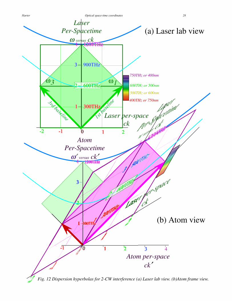
Fig. 12 shows the plots of per-spacetime “baseball diamond” coordinates for comparison of lab
and atom frame views. While Fig. 12a is a “blimp’s-eye view” of the lab-frame diamond in Fig. 6, the
atom frame view in Fig. 12b looks like the baseball field seen by a spectator sitting in the stands above
the dugout. Nevertheless, identical hyperbolas are used to mark grids in both views.
Each point on the lower hyperbola is a bottom point =B=2 (600THZ) for the frame whose
relative velocity u makes it a -axis (k =0)-point, and every (k =0)-point on the upper hyperbola is its
bottom point =2B=4 (1200THZ), and so on for hyperbolas of any given proper frequency value .
The same applies to space-time plots for which time ct takes the place of per-time and space x takes
the place of per-space ck . Then bottom points are called proper time or -values from (2.21).
For single CW light the proper time must be constant since a single CW cannot age. It is a
convention to make the baselines or light cone intersect at the origin in both time and space. This sets
the baseline proper time constant to zero. Then invariants (2.21) reduce to baseline equations x=±ct or
x =±ct for all frames. The space-time light cone relations are in direct correspondence with the per-
space-time light cone relations =±ck or =±ck for zero proper frequency in all frames and are
concise restatements of the Evenson CW axiom (1.1).
Harter Optical space-time coordinates 28
−
−
4 −
Laser per-spaceck
ω1ω3750THz or 400nm
600THz or 500nm
500THz or 600nm
400THz or 750nm1s
t bas
eline3rd baseline
−
−
4 −
Atom per-spaceck
4 −
Laser per-space
ck
4
(a) Laser lab view
(b) Atom view
Fig. 12 Dispersion hyperbolas for 2-CW interference (a) Laser lab view. (b)Atom frame view.
−
Laser
Per-Spacetime
w versus ck
LaserPer-Spacetime
ω versus ck
AtomPer-Spacetime
ω versus ck
ωθωερτψυιοπ
Harter Optical space-time coordinates 29
3. Mechanics by CW axioms
Each of the 2-CW structures or properties discussed so far are due to relative interference
effects between pairs of single CW entities that, by themselves, lack those properties. Single CW plane
waves have no proper invariant frequency, no rest frame, and no velocity less than the unreachable c.
To acquire such properties there must be an interference encounter or pairing with another CW.
Two-CW interference acquires other important properties including classical and relativistic
mechanics of mass, energy, momentum that characterize a quantum matter wave. Such acquisition is
from hyperbolic phase relations (2.19-20) that, in turn, follow from CW axioms (1.1) and (1.2).
p = B cosh
B +1
2B 2 (for u c)
(3.1a)
ckp = Bsinh
B (for u c)(3.1b)
u
c= tanh
(for u c)
(3.1c)
Here B= . The first two are components ( p,ckp) of the P-vector in Fig. 11, and u/c is the tangent slope
at P. At low group velocity (u c) rapidity approaches u/c, and p and kp are simple functions of u.
p B +1
2
B
c2u2 (3.2a)
kpB
c2u (3.2b)
We note that these ( p,ckp) functions fit classical Newtonian-energy E and Galilean-momentum p.
E = const.+1
2Mu2 (3.3a) p Mu (3.3b)
Multiplying wave results (3.2) by a single scale factor s=Mc2/B gives classical definitions (3.3).
E = s p sB +1
2
sB
c2u2 (3.4a)
p = skpsB
c2u (3.4b)
Newton’s const in E (3.3a) is moot; only energy difference E counts. But, in (3.4a) const.=sB is the
proper-frequency value B= of Fig. 11b scaled to sB=s . It is also the famous Einstein rest energy.
const.= sB = Mc2 = s (3.4c)
Then exact relativistic Planck-DeBroglie quantum scaling laws follow from exact CW results (3.1).
E = s p = Mc2 cosh =Mc2
1 u2 / c2(3.5a) p = skp = Mcsinh =
Mu
1 u2 / c2(3.5b)
Scale factor s in Planck17
E=s or DeBroglie18
p=sk laws is found by experiment. The lowest
observed s-value is the Planck angular constant =1.05·10-34
J·s in Planck’s original law E= N=hN for
N=1. Integer N is a light-quantum-number or photon-count discussed in Sec. 6. (Occam’s razor is used
again to further slice classical CW’s into N-photon waves belonging to nets of ( N,ckN)-hyperbolas.)
Each photon of a 2-CW cavity adds a tiny mass M = /c2= (1.2·10
-51)kg to the cavity but p is
zero. A single free CW has no rest mass but its momentum p = k= /c= (3.5·10-43
)kg·m·s-1from (3.5b)
is p =M c. It is small, too, but M times c is not as tiny as M and it resembles Galileo’s relation (3.3b).

Harter Optical space-time coordinates 30
Definitions of wave mass
If mass or rest energy is due to proper phase frequency , then a quantum matter wave has
mass without invoking hidden Newtonian “stuff.” There is a certain Occam-like economy in the fact
that two CW’s of light give exact classical mass-energy-momentum relations (3.5). However, a CW
theory exposes multiple definitions of mass that a Newtonian theory would not distinguish.
First, the Einstein-Planck wave frequency-energy-mass equivalence relation (3.4c) ascribes rest
mass M rest to a scaled proper frequency s /c2. The scale factor s is Planck’s s= N for cavity mode N.
Mrest = E / c2
= N / c2 (3.6)
For rest electron mass me =9.1·10-31
kg or Mp =1.67·10-27
kg of a proton, the proper frequency times N=2 is
called zwitterbevegun (“trembling motion”) and is as mysterious as it is huge. (Electron rest frequency
e = me c2/ =7.76·10
+20(rad)s
-1 is the Dirac (e+e )-pair production
19 threshold as discussed in Sec. 6.)
Second, define momentum-mass Mmom by ratio p/u of momentum (3.5b) to velocity u. (Galileo’s
p=Mmomu) Now Mmom varies as cosh e / 2 at high rapidity but approaches invariant Mrest as 0 .
p
uMmom =
Mrestc
usinh = Mrest cosh
u cMreste / 2
= Mrest 1 u2 / c2u c
Mrest
(3.7)
Frame velocity u is wave group velocity and the Euclid mean construction of Fig. 11a shows u is the
slope of the tangent to dispersion function (k). A derivative of energy (3.5a) verifies this once again.
Vgroup =d
dk=
dE
dp=
c2 p
E= u (3.8)
Third, define effective-mass Meff as ratio p / u =F/a of momentum-change to acceleration.
(Newton’s F=Meffa) Meff varies as cosh3 e3 / 2 at high rapidity but is invariant Mrest as 0 .
F
aMeff
dp
du=
dk
dVgroup
=d
dk
d
dk=
d 2
dk 2
= Mrest 1 u2 / c2( )3/2
u cMrest
(3.9)
Effective mass is divided by the curvature of dispersion function, a general quantum wave
mechanical result. Geometry of a dispersion hyperbola =Bcosh is such that its bottom (u=0) radius of
curvature (RoC) is the rest frequency B=Mrestc2/ , and this grows exponentially toward as velocity u
approaches c. The 1-CW dispersion ( =±ck) is flat so its RoC is infinite everywhere and so is photon
effective mass (Meff( )= ) consistent with the (All colors go c)-axiom (1.1). The other extreme is photon
rest mass (Mrest( )=0. Between these extremes, photon momentum-mass depends on CW color .
Mrest( )=0 (3.10a) Mmom( )=p/c= k/c= /c2 (3.10b) Meff( )= (3.10c)
For Newton this would confirm light’s “fits” to be crazy to the point of unbounded schizophrenia.
Harter Optical space-time coordinates 31
Absolute vs. relative phases
Probably Newton would find a CW theory to be crazy. Claiming that heavy hard matter owes
its properties to rapid hidden phase oscillations would not elicit a Newtonian invitation to the Royal
Society but rather to a lunatic asylum. Even though CW results (3.2) give Newtonian axioms (3.3) at
low speeds, the result would seem to fail at high speeds where exact results (3.5) sag below Newton’s.
Also, the enormous constant Mc2 in the energy would, in 1670, seem meaningless.
Not until 190520
does Einstein’s theory appear with energy sag and Mc2. Yet Einstein’s classical
training left him leery of hidden quantum wave phases with dicey interpretations of intensity as
probability. Also, he may have asked why observable results depend on a square =| |2 that kills the
overall phase frequency, seemingly losing the one quantity that represents (or is) the total energy.
Square | |2 of a 2-CW =e
ia+e
ib loses phase factor ei(a+b)/2 leaving only group functions cos2 ( 2a b )
of differences 1 3 or k1 k3 of 1st and 3
rd base frequencies or k-vectors. Group beat frequency
= 1 3 is zero in the rest frame of Fig. 6c where it is a stationary wave. In Fig. 7c or any other
frame, | |2 is not stationary but is observed to have velocity Vgroup 0. Fourier sums of m=3 or more
terms = a1ei(k1x 1t )
+ a2ei(k2x 2t )+ a3e
i(k3x 3t )+ ... may have multiple beats in * as in Fig. 7d.
P =| |2= * = ai * ajei( kij x ij t)
(3.11)
With m(m 1) / 2 observable difference ij = 1 j or beat notes, P cannot rest in any frame.
Differences or derivatives are observable while absolute -frequency stays hidden until two quantum
objects interfere. Then new beats arise from differences between the two absolute frequencies and old
ones. A new absolute phase (not in | |2) is the sum of them all. Limiting observation to beats or relative
frequency may be a quantum version of Einstein’s popularized saw, “It’s all relative.” (Phase velocity
may escape with its Galilean arithmetic intact, but here it finally surrenders its absolutes to relativism.)
Total phase gives total energy E or momentum p, but differentials are what one feels through
work E or impulse p. Invariant quantities like and Mrest depend on total phase but intensity (3.11)
has only differentials or relative beats. Among frame-dependent relative quantities are group velocity u
(3.8), Mmom (3.7), and Meff (3.9). But, rest mass Mrest (3.4c) is a frame-invariant absolute quantity. Recall
however that Mmom and Meff approach Mrest at zero velocity. (While | |2 may register a beat with a DC
(static 0=0) wave, lack of resonance confines ( 0=0)-carrier waves to beat only locally.)
The phase frequency p in a quantum wave eip cos g = ei(kp x pt)
cos(kgx
gt) is like a carrier
frequency of a radio wave, fast and silent. The group frequency g is like the audible signal, much
slower and heard in resonant beats a b involving carrier and receiver. Atomic “carrier” frequencies
p=Mpc2/ due to rest mass are enormous as are those of atomic measuring devices that play the role of
“receivers” in quantum experiments. Measurement involves resonant contact of an atom and devices
that horse-trade beats much faster than even those achieved by Evenson or any laser technology so far.

Harter Optical space-time coordinates 32
One way to avoid huge Mc2/ -related phase frequencies is to ignore them and approximate the
relativistic equation E=Mc2cosh of (3.5a) by the Newtonian approximation (3.4a) that deletes the big
rest-energy constant sB=Mc2. The exact energy (3.5a) that obeys CW axioms (1.1) is rewritten in terms
of momentum (3.5b) in (3.12). Then (3.13) gives the Newtonian approximation with Mc2 deleted.
E =Mc2
1 u2 / c2= Mc2 cosh = Mc2 1+ sinh2
= Mc2( )2+ cp( )
2(3.12)
E = Mc2( )2+ cp( )
21/2
Mc2+
1
2Mp2
S approx
1
2Mp2 (3.13)
Since only frequency differences affect an observation based on | |2 (3.11), the energy origin may be
dropped from (E=Mc2, cp=0) to (E=0, cp=0). (Frequency is relative!) Hyperbola (3.12) is then Newton’s
parabola (3.13) for momentum p=Mu much less than Mc, or u much less than c.
Group velocity u=Vgroup=dkd of (3.8) is a relative or differential quantity so origin shifting does
not affect it. However, phase velocity k =Vphase is greatly reduced by deleting Mc2 from E= . It slows
from Vphase=c2/u that is always faster than light to a sedate sub-luminal speed of Vgroup/2. Having Vphase go
slower than Vgroup is an unusual situation but one that has achieved tacit approval for Bohr-Schrodinger
matter waves.21
The example used in Fig. 4 is a 2-CW matter wave exhibiting this.
Standard Schrodinger quantum mechanics, so named in spite of Schrodinger‘s protests22
, uses
Newtonian kinetic energy (3.13) (or (3.3) with potential (as the const.-term) to give a Hamiltonian.
H=p2/2M + or: =
2k
2/2M + k (3.14)
The CW approach to relativity and quantum exposes some problems with such approximations.
First, a non-constant potential must have a vector potential A so that ( ,cA) transform like
( ,ck) in (2.10a) or (ct,x) in (2.10b) or as (E,cp) with scaling laws p= k and E= . Transformation
demands equal powers for frequency (energy) and wavevector (momentum) such as the following.
(E- )2=(p-cA)
2/2M+Mc
2 or: ( - k)
2= ( k-cA)
2/2M+Mc
2 (3.15)
Also, varying potentials perturb the vacuum so single-CW’s may no longer obey axioms (1.1-2).
Diracs’s elegant solution obtains ±pairs of hyperbolas (3.12) or (3.15) from avoided-crossing
eigenvalues of 4x4 Hamiltonian matrix equations. These ideas require three-dimensional wavevectors
and momenta as will be introduced later. First, the more fundamental Lagrangian geometry of quantum
phase will be used to relate relativistic classical and quantum mechanics.

Harter Optical space-time coordinates 33
4. Classical vs. quantum mechanics
The CW-spectral view of relativity and quantum theory demonstrates that wave phase and in
particular, optical phase, is an essential part of quantum theory. If so, classical derivation of quantum
mechanics might seem about as viable as Aristotelian derivation of Newtonian mechanics.
However, the 19th
century mechanics of Hamilton, Jacobi, and Poincare developed the concept
of action S defined variously by area
pdq in phase-space or a Lagrangian time integral Ldt . Action
definition begins with the Legendre transformation of Lagrangian L and Hamiltonian H functions.
L = p x H (4.1a)
L is an explicit function of x and velocity u = x while the H is explicit only in x and momentum p.
0 =L
p (4.1b)
p =L
x (4.1c)
0 =H
x (4.1d)
x =H
p (4.1e)
Multiplying by dt gives the differential Poincare invariant dS and its action integral S = Ldt .
dS = L dt = p dx H dt (4.2a) S = L dt = p dx H dt (4.2b)
Planck and DeBroglie scaling laws p= k and E= identify action S as scaled quantum phase .
d = L dt = k dx dt (4.3a)
= k dx dt (4.3b)
If action dS or phase d is integrable, then Hamilton-Jacobi equations or (k, ) equivalents hold.
S
x= p (4.4a)
S
t= H (4.4b)
x= k (4.4c)
t= (4.4d)
Phase-based relations (4.4c-d) define angular frequency and wave number k. The definition (3.8) of
wave group velocity is a wave version of Hamilton’s velocity equation (4.1e).
x =H
p equivalent to: u = V
group=
k
The coordinate Hamilton derivative equation relates to wave diffraction by dispersion anisotropy.
p =H
x equivalent to:
k =x
Classical HJ-action theory was intended to analyze families of trajectories (PW or particle
paths), but Dirac and Feynman showed its relevance to matter-wave mechanics (CW phase paths) by
defining an approximate semi-clasical wavefunction based on the Lagrangian action as phase.
ei= eiS /
= ei L dt / (4.5)
The approximation symbol ( ) indicates that only phase but not amplitude is assumed to vary here. An
x-derivative (4.4a) of semi-classical wave (4.5) has the p-operator form in standard quantum theory.
x
i S
xeiS /
=i
p (4.6a) i x
= p (4.6b)

Harter Optical space-time coordinates 34
The time derivative is similarly related to the Hamiltonian operator. The H-J-equation (4.4b) makes
this appear to be a Schrodinger time equation.
t
i S
teiS /
=i
H (4.7a)
it
= H (4.7b)
However, this approximation like that of (3.14) ignores relativity and lacks the economy of logic shed
by light waves. The Poincare phase invariant of a matter-wave needs re-examination.
Contact transformation geometry of a relativistic Lagrangian
A matter-wave has a rest frame where x =0=k and its phase = kx- t reduces to μ , a product
of its proper frequency μ = N (or Mc2/ ) with proper time t = . Invariant differential d is reduced, as
well, using the Einstein-Planck rest-mass energy-frequency equivalence relation (3.4c) to rewrite it.
d = kdx dt= μ d = -(Mc2/ ) d . (4.8)
-Invariance (2.21) or time dilation in (2.10b) gives proper d in terms of velocity u =dx
dt and lab dt.
d = dt (1-u2/c
2) )=dt sech (4.9)
Combining definitions for action dS=Ldt (4.2) and phase dS = d (4.3) gives the Lagrangian L.
L = μ = -Mc2
(1-u2/c
2)= -Mc
2sech (4.10)
Fig. 13 plots this free-matter Lagranian L next to its Hamiltonian H using units for which c=1=M.
(a) Hamiltonian
Momentum p
P
P′
P′′
-L-L′
-L′′
L(q,q)Velocity u=q
QQ′
Q′′
-H
-H′
-H′′
H H′
H′′L
L′L′′
H
H′
H′′
slope:
slope:∂H∂p
= q= u
∂L∂q
= p
(b) LagrangianH(q,p)
radius = Mc2
O
O
Fig. 13. Geometry of contact transformation between relativistic (a) Hamiltonian (b) Lagrangian
The relativistic matter Lagrangian in Fig. 13b is a circle. Three L-values L, L , and L in Fig.
13 are Legendre contact transforms of the three H-values H , H , and H on the Hamiltonian hyperbola
in Fig. 13a. Abscissa p and ordinate H of a point P in plot (a) gives negative intercept -H and slope p of
the tangent contacting the transform point Q in plot (b) and vice-versa. Contact geometry shows a
structure of wave-action-energy mechanics. Lagrange kinetic energy L =21 Mu2 equals H = p2 / 2M of

Harter Optical space-time coordinates 35
Hamilton with p = Mu as hyperbola H and circle L both approximate a Newton parabola at low speed
u<<c in Fig. 13. But, as u nears c the L-circle rises and the H-hyperbola sags to meet its c-asymptote.
Action integral S= Ldt is to be minimized. Feynman’s interpretation of S minimization is
depicted in Fig. 14. A mass flies so that its “clock” is maximized. (Proper frequency μ = Mc2 / is
constant for fixed rest mass, and so minimizing μ means maximizing + .) An interference of Huygen
wavelets favors stationary and extreme phase and the fastest possible clock as is sketched in Fig. 15.
Feynman imagines families of classical paths or rays fanning out from each space-time point on a
wavefront of constant phase or action S. Then, according to a matter wave application of Huygen's
principle, new wavefronts are continuously built in Fig. 15 through interference from “the best” of all
the little wavelets emanating from a multitude of source points on a preceding wavefront. The result is
a classical momentum normal to each wavefront given by p= S or (4.4a) for the “best” ray.
The “best” are so-called stationary-phase rays that are extremes in phase and thereby satisfy
Hamilton's Least-Action Principle requiring that Ldt is minimum for “true” classical trajectories. This
in turn enforces Poincare' invariance by eliminating, by de-phasing, any “false” or non-classical paths
because they do not have an invariant (and thereby stationary) phase. “Bad rays” cancel each other in a
cacophonous mish-mash of mismatched phases. Each Huygen wavelet is tangent to the next wavefront
being produced. That contact point is precisely on the ray or true classical trajectory path of minimum
action and on the resulting “best” wavefront. Time evolution from any wavefront to another is thus a
contact transformation between them described by the geometry of Huygens Principle.
Thus a Newtonian clockwork-world appears to be the perennial cosmic gambling-house winner
in a kind of wave dynamical lottery on an underlying wave fabric. Einstein’s God may not play dice,
but some persistently wavelike entities seem to be gaming at enormous Mc2/ -rates down in the cellar!
It is ironic that Evenson and other metrologists have made the greatest advances of precision in
human history, not with metal bars or ironclad classical mechanics, but by using the most ethereal and
dicey stuff in the universe, light waves. This motivates a view of classical matter or particle mechanics
that is more simply and elegantly done by its relation to light and its built-in relativity, resonance, and
quantization that occurs when waves are subject to boundary conditions or otherwise confined. While
Newton was complaining about the seeming “fits” of light, it was just trying to tell him something.
Derivation of quantum phenomena using a classical particle paradigm appears a doomed effort.
If particles are made by waves, optical or otherwise, rather than vice versa as Newton believed, the case
is closed. Also, CW trumps PW as CW symmetry axioms (1.1-2) derive classical results (3.4) with
exact relativity and quantum relations (3.5) tossed in the bargain. Such Occam economy is not found
on a PW path from Newton to Einstein and Planck. This leaves the basic CW sum-and-difference
phase relations that seem to underlie physics and Poincare contact geometry. They are clarified next.

Harter Optical space-time coordinates 36
Clock on natural
runs the fastest
Clocks on
are neitherslowest norfastest
Clock on light-cone pathis stopped
Space x
Time ct
...is stopped
...neitherslowest norfastest
Fig. 14 “True” paths carry extreme phase and fastest clocks. Light-cone has only stopped clocks.
Mostly destructiveinterference
Stationary phase
by constructiveinterference
Fig. 15 Quantum waves interfere constructively on “True” path but mostly cancel elsewhere.

Harter Optical space-time coordinates 37
Geometry of circular and hyperbolic functions
Geometry of half-sum and half-difference phase P=(R+L)/2 and group G=(R-L)/2 vectors is
based on trigonometric exponential identities that are crown jewels of 18th
century mathematics and
have Euclidian geometric origins shown in Fig. 16. Phase angle- identities apply to Fig. 16a.
e+i= cos + i sin
e i= cos i sin
(4.11a)cos = (e+i
+ e i ) / 2
i sin = (e+i e i ) / 2(4.11b)
The circular function tan is named for a tangent to a unit circle shown in Fig. 16(a). Its incline (sine)
elevation is sin . The complimentary tangent or cotangent cot completes the tangent distance between
axes where is circle arc-length- or subtended area- . Hyperbolic functions use area for “angle.”
e+ = cosh + sinh
e = cosh sinh(4.11c)
cosh = (e+ + e ) / 2
sinh = (e+ e ) / 2(4.11d)
Fig. 16b shows how hyperbolic functions relate to circular ones in Fig. 16a. The circular sine equals
the hyperbolic tangent (sin =tanh ) and vice versa (tan =sinh ). Each circular function has a segment
that matches one for a hyperbolic function, for example (cos =sech ). These relations recap the CW
view of the Legendre contact transformation in Fig. 13 that underlies classical and quantum theory that
is the algebra and geometry for every bit of light-and-matter in and around us!
In Fig. 16, circular area and hyperbolic area have been chosen so that tan =1.15=sinh and
sin =0.75=tanh , that is for u=3c/4. The tangent to the circle in Fig. 16a-b is like the one that contacts
the Lagrangian circle in Fig. 13b to contact-transform it to the Hamiltonian hyperbola in Fig. 13a, and
vice versa the hyperbolic tangent in Fig. 16b is like the one that transforms the Hamiltonian hyperbola
in Fig. 13a to the Lagrangian circle in Fig. 13b.
The hyperbolic tangent u/c=tanh of (2.19) corresponds to frame rapidity and group velocity
u=Vgroup =dkd in (2.8), (3.8) and in Fig. 11a-b. The circular tangent angle or inclination sin belongs to
Lagrangian velocity function (4.10) in Fig. 13b. (The horizontal axis of the latter in the vertical axis of
Fig.11. This geometry is symmetric to axis-switching.) As u and approach c and , respectively, the
circular angle approaches /2. This angle is the stellar velocity aberration angle, that is, the polar
angle that vertical starlight is seen by a horizontally moving astronomer to tip into her direction of
motion. Aberration angle , like rapidity , is 1st-order in velocity u and equal u/c to low speeds.
Most of the twelve circular-hyperbolic trigonometric ratios in Fig. 13 belong to one or more
physical or geometric effects shown in prior diagrams beginning with Euclid’s rectangle-in-circle
mean construction of Fig. 10. If prior ratio constructions are overlapped in the form of Fig. 13 there
results in Fig. 17a what might be described as a global ratio riot. This riot is simplified and labeled in
zoom-in views of Fig. 17b-d and they are the basis of the following discussion of the role of tangent-
contact geometry in CW analysis of Poincare contact transformation and relativistic quantum waves.

Harter Optical space-time coordinates 38
ct (time)
x(space)
1.0
-1.0
1.0
ρ
1
coshρ
sinhρ
cothρ
cschρ
cschρe+ρ
sechρ
tanhρ
tanhρ
sinhρ
coshρ
Hyperbolic arc areaρ =1.0434=rapiditysinh ρ =1.2433cosh ρ =1.5955tanh ρ =0.7792csch ρ =0.8043sech ρ =0.6267coth ρ =1.2833
x
y
1.0
1.0
1
Circlular arc area(a) Circlular Functions (plane geometry)
(b) Hyperbolic Functions (spacetime geometry)
e-ρ
e-ρ
e-ρ
e-ρ
e-ρ
Fig. 16 Trigonometric geometry (a) Unit circular area =0.86 and (b) Unit hyperbolic area =0.99.

Harter Optical space-time coordinates 39
Hyper-circular contacts
Beginning with the Euclidian mean diagram of Fig. 10, three mean frequencies arise from an
interfering pair of left-moving “red” and right-moving “blue” beams of frequency L and R. First is a
half-sum phase frequency p=( R+ L)/2 (arithmetic mean) that defines the circle radius in Fig. 10.
Second is a half-difference group beat frequency g=( R- L)/2 (difference mean) that is radial distance
of circle center to origin. Third is a root-product proper frequency =( R· L)1/2 (geometric mean) that
is the base radius or bottom of a (k) hyperbola of rest energy B= =Mc2 above origin in Fig. 11.
Phase and group frequencies are defined as ratios or shifts of the geometric mean frequency ,
and this begins with the Doppler shift definition of the red L=e and blue R=e+ CW components.
Ratio values p= cosh and g= sinh define each point on a -hyperbola dispersion curve in Fig. 17.
Fig. 17 is based on circles with three different radii, one for each mean frequency. The base
circle-b drawn centered at origin has radius B= =Mc2 of the Lagrangian circle in Fig. 13b. A smaller
circle-g has group radius g=Bsinh . A larger circle-p has phase radius p=Bcosh of the Euclidean
circle in Fig. 10 and is drawn with dashed lines in Fig. 17. (Base value B is scaled for energy here.)
Circle-p of larger radius p=Bcosh is centered at cp= g=Bsinh , a horizontal distance equal
to the radius of the smaller circle-g, while the latter is centered at E= p=Bcosh , a vertical distance
equal to the radius of the larger circle-p. Tangents contacting the circles or the hyperbola define most of
the physical quantities labeled in the zoom-in view of Fig. 17b. Intersections and chords shared by two
of the circles also provide the key quantities as seen in Fig. 17a.
So far the CW development has emphasized the Doppler ratio as a starting point beginning with
Fig. 7 and culminating with the Euclidean means of Fig. 10. However, most developments of relativity
start with velocity u, and that geometric approach is excerpted in a simplified construction of Fig. 17c
where u/c=45/53 and Fig. 17d where u/c=3/5. (Fig. 17a-b and most other figures use u/c=3/5.) Once the
velocity u/c line intersects the basic b-circle and its horizontal tangent of unit-energy (B=1=Mc2), it
only takes three more lines to derive Lagrangian -L=Bsech , then momentum cp=Bsinh , and finally the
Hamiltonian H=Bcosh . Then a compass is used to check accuracy with the phase p-circle by making
sure it goes from (cp,H) to the (0,B)-point on top of the b-circle. The p-circle goes on to intersect the
negative cp-axis at the Doppler red shift rB=Be+ . Finally, the group g-circle in Fig. 17a-b has a chord
intersection with the p-circle that is the hyperbolic contact tangent, and it grazes the -angle normal to
the Lagrangian circle tangent in Fig. 17b. This helps to clarify geometry of H-L contact transformations
introduced in Fig. 13. The construction also applies to the space-time domain.
If Fig. 17 is in space-time, the segment -L=Bsech is Lorentz contraction = B 1 u2 / c2 . The
H=Bcosh and cp=Bsinh segments are, respectively Einstien time dilation d = B / 1 u2 / c2 and
asimultaneity a=ud/c coefficients. Node-to-node or peak-to-peak gaps contract by =4/5 in Fig. 7d-e.

Harter Optical space-time coordinates 40
ρ
ρρ
ρ
φ
−
4
4
ρ
ρ cp
H=E
ρ
ρ
(a) Geometry of relativistic transformation and wave based mechanics
(b) Tangent geometry (u/c=3/5)
(c) Basic construction given u/c=45/53
u/c =3/5u/c =1
cp =3/4
H =5/4
-L =4/5
cp =45/28
H =53/28
-L=28/45
e-ρ=1/2e-ρ=2/7
(d) u/c=3/5
11
1 1
g-circle
p-circle
Fig. 17 Relativistic wave mechanics geometry. (a) Overview. (b-d) Details of contacting tangents.
As speed reduces in Fig. 17c-d from u/c=45/53 to u/c=3/5 or to lower values, the Lagrangian
velocity angle and Hamiltonian rapidity approach the velocity ratio u/c. Galilean velocity addition
rules resume. In the opposite ultra-relativistic regime, approaches /2, approaches , and u/c nears
unit slope or 45° in Fig. 17c. But, Galilean-like rules (2.16) apply to rapidity at all speeds (so far).

Harter Optical space-time coordinates 41
5. Symmetry and conservation principles
In Newtonian theory the first law or axiom is momentum conservation. Physical axioms, by
definition, have only experimental proof. Logical proof is impossible unless a theory like Newton’s
becomes sub-summed by a more general theory with finer axioms. Proof of an axiom undermines it so
it becomes a theorem or result of more basic axioms. (Or else an axiom might be disproved or reduced
to an approximate result subject to certain conditions.)
The logic of axioms yielding results or theorems in mathematical science probably goes back
two thousand years to the time of Euclid’s Elements. Also, axiomatic approaches to philosophy and
natural science show up in writings as early as that of Occam or even Aristotle, but it is not until the
European Renaissance that experiments are precise enough to support mathematical models. By the
European Enlightenment period, mathematical logic of physical science had become more effective
and productive than any preceding philosophy due in no small part to increasingly precise evidence.
As stated in the introduction, current time and frequency measurements have achieved almost
unimaginable precision. Based on this, two continuous wave (CW) axioms (1.1-2) have been used to
undermine Newtonian axioms concerning mass, energy, and momentum so they became approximate
results (3.2) and give rise to exact equivalents of Newtonian concepts in Einstein and Planck relativity
and quantum theory in (3.5). That is a modern example of an Occam razor-cut undermining axioms.
The undermining of Newton’s first axiom (momentum conservation) by the shaved CW axioms
is a good example to expose the logic involved. CW logic leads to the DeBroglie scaling law (3.5b)
that equates momentum p to wavevector k scaled in units. A rough statement of how CW axioms
undermine or “prove” p-conservation axioms is that k-conservation is required by wave coherence and
so p= k must be conserved, as well. However, that oversimplifies a deeper nature of this logic.
The strength (and also, weakness) of CW axioms (1.1-2) is that they are symmetry principles
due to the Lorentz-Poincare isotropy of space-time that invokes invariance to translation T( , ) in the
vacuum. Operator T has plane wave eigenfunctions k , = Aei(kx t) with eigenvalues ei(k ) .
T k , = ei(k )k , (5.1a) k , T†
= k , e i(k ) (5.1b)
This also applies to 2-part or “2-particle” states K , = k1, 1 k2 , 2 where exponents add (k, )-values of
each constituent to K=k1+k2 and = 1+ 2, and T( , ) -eigenvalues also have the form ei(K ) of (5.1).
Matrix K , U
K , of T-symmetric evolution U is zero unless K = k1 + k2 = K and = 1 + 2 = .
K , UK , =
K , T† ( , )UT( , )K , (if UT = TU for all and )
= e i(K )ei(K )K , U
K , = 0 unless: K = K and: =
(5.2)
T-symmetry requires total energy E = and total momentum P = K be conserved for archetypical
CW states, but laboratory CW have momentum uncertainty k=1/ x due to finite beam size x and
energy uncertainty due to time limits. Newton’s 1st law is verified but only as an ideal limit.

Harter Optical space-time coordinates 42
Symmetry is to physics what religion is to politics. Both are deep and grand in principle but
roundly flaunted in practice. Both gain power quickly by overlooking details. In Sec. 3 relativistic and
quantum kinetic properties of a massive “thing” arise from those of an optical 2-CW function in one
space dimension. This means that mass shares symmetry with 2-CW light, not that mass is 2-CW light.
Massive “things” do not vanish if the light is turned off as does a tiny optical mass N /c2 of a cavity.
Puzzling questions remain. Why do simple wave optics lead directly to general properties (3.5)
of relativity and quantum mechanics of a massive particle? How does a cavity of counter-propagating
green light waves act like it holds particles of mass M= /c2?
The short answer to one question is that particles are waves, too, and so forced by Lorentz
symmetry to use available hyperbolic invariants
2 (ck)2= (Mc2 / )2 for dispersion. To answer the
second question entails further loss of classical innocence. In Sec. 6 Occam’s razor is again applied to
cut semi-classical CW laser fields down to single field quanta
or photons. So the second short
answer is that waves are particles, too, even for optical dispersion ( 2 (ck)2= 0) .
By many accounts, quantum theory begins with Planck’s axiom E= N . This is distinguished
from the scaling law E=s derived in (3.5) since its scale factor s= N is not an obvious consequence of
CW phase axioms (1.1-2) that lead to (3.5). CW logic seems to require additional axioms involving
Maxwell energy E and field amplitude quantization by Planck. This is discussed shortly.
Quantization of phase variables
Waves were known to resonate at discrete wave numbers km = m L2
= mk1 in rings or boxes of
fixed length L. The DeBroglie relations between k and momentum p force quantization pm = km = mp1
where momentum quantum numbers23
m=0, ±1, ±2,… count waves on ring L as in Bohr models. Planck
dispersion E
m= (k
m) (3.5) gives energy levels Em = m2E1 for sub-relativistic cases with E1 = p1
2 / 2M .
Heisenberg24
showed quanta pm or Em arise from eigenvalues (literally “own-values”) of matrix
operators p or H whose eigenvectors (“own-vectors”) pm or Em may be superimposed.
= 1 E1 + 2 E2 + 3 E3 + … (5.3)
(Dirac’s bra-ket25
notation came later.) Allowing things to be at (or in) m places (or states) allows mean
values E = H to range continuously from lowest quantum levels E1 to the highest Em .
E = H = 1
2E1 + 2
2E2 + 2
2E2 + … (5.4)
For classicists, the notion that each multiple-personality-k has a probability k
2seems, if not crazy,
then at least dicey in the sense of Einstein’s skeptical quote, “God does not play dice…” 26
But, superposition is an idea borrowed from classical waves, and their interference makes them
ultra-sensitive to relative position and velocity, a first order sensitivity that leads elegantly to relativity
transformation (2.10) and kinematic relations (3.5) by geometry of optical phase kx- t. But, amplitude
“A” of wave (1.9) or (1.10) is set arbitrarily. It is ignored in (4.5). Without Maxwell and Planck rules,
CW amplitude or wave quantity is undefined and un-quantized. This must now be discussed.

Harter Optical space-time coordinates 43
6. Variation and quantization of optical amplitudes
What is deduced from wave phase alone? Wave amplitude has so far been skirted for Occam economy:
“Pluralitas non est ponenda sine neccesitate” (Do not assume plurality without necessity.) CW phase axioms
(1.1-2) give Lorentz-Doppler and Planck-DeBroglie symmetry relations yet 2-CW amplitudes (1.10)
are not defined beyond assuming their 1-CW amplitudes match. Standing wave grid reference frames
in Fig. 6 and Fig. 7 are just points where amplitude is zero, that is, loci of real wave function roots.
Discussion of non-zero amplitude variation begins with counter-propagating 2-CW dynamics
involving two 1-CW amplitudes A and A that are unmatched. (A A )
A ei(k x t)+ A ei(k x t)
= ei(k x t)[A ei(k x t)+ A e i(k x t) ] (6.1a)
Half-sum mean phase rates (k , ) and half-difference means (k , ) appear here as in (1.10).
k = (k + k ) / 2
= ( + ) / 2(6.1b)
k = (k k ) / 2
= ( ) / 2(6.1c)
Also important is amplitude mean A = (A + A ) / 2 and half-difference A = (A A ) / 2 . Wave
motion depends on standing-wave-ratio SWR or the inverse standing-wave-quotient SWQ affects.
SWR =(A A )
(A + A )(6.2a) SWQ =
(A + A )
(A A )(6.2a)
Recall mean frequency ratios for group velocity (2.7b) or its inverse that is phase velocity (2.7a).
Vgroup =k
= c( )
( + )(6.3a) Vphase = k
= c( + )
( )(6.3b)
A 2-state amplitude continuum is bounded by (A = 1, A = 0) a pure right-moving 1-CW of SWR=1 and
a pure left-moving 1-CW (A = 0, A = 1) of SWR=-1. A 2-CW standing-wave (A =2
1= A ) has SWR=0.
Wave paths for various SWR values are drawn in Fig. 18 for 600THz 2-CW pairs and in Fig. 19
for Doppler shifted 300THz and 1200THz 2-CW pairs at the same SWR values. The SWQ is the ratio of
the envelope peak (interference maximum) to the envelope valley (interference minimum), and vice
versa for SWR=1/SWQ. Single frequency 2-CW paths of nonzero-SWR in Fig. 18 do a galloping motion.
Each wave speeds up to peak speed c/SWR=c·SWQ as it first shrinks to squeeze through its envelope
minima and then slows to resting speed c·SWR as it expands to its maximum amplitude. Only at zero-
SWR do 2-CW zero-paths appear to travel at a constant group speed (6.3a) and phase speed (6.3b) as in
Fig. 18c or 19c. (For 1-CW paths or unit SWR=±1 there is just one speed ±c by axiom (1.1).)
The real and imaginary parts take turns. One gallops while the other rests and vice versa and
this occurs twice each optical period. If frequency ratio (6.3) and amplitude ratio (6.2) have opposite
signs as in Fig. 18c (±0 or ± ) and in Fig. 19e (±3/5 or ±5/3), wave zero paths will follow a right angle
staircase. 1-frequency staircase (Vgroup=0=SWR) in Fig. 18c is a Cartesian grid like Fig. 6c. 2-frequency
waves (Vgroup 0) have Minkowski grids like Fig. 7c for SWR=0 or quasi-Cartesian stair steps like Fig.
19e for Vgroup=-cSWR. To broadcast Cartesian grids to a u-frame one tunes both Vgroup and cSWR to u.

Harter Optical space-time coordinates 44
(a) - =0.2
- =0.8SWR=+3/5
(b) - =0.4
- =0.6
(c) - =0.5
- =0.5
(e) - =0.8
- =0.2
(d) - =0.6
- =0.4 SWR=-1/5
SWR=0
SWR=+1/5
1-frequencycases
ω =2c, k =2,
ω =2c, k =-2
uGROUP=0
uPHASE
SWR=-3/5Fig. 18 Monochromatic (1-frequency)2-CW wave space-time patterns.
(a) - =0.2
- =0.8
(b) - =0.4
- =0.6
(c) - =0.5
- =0.5
(d) - =0.6,
- =0.4
(e) - =0.8
- =0.2
ω =4c, k =4
ω =1c, k =-1
uGROUP/c=3/5
uPHASE/c=5/3
SWR=+3/5
SWR=+1/5
SWR=0
SWR=-1/5
SWR=-3/5
2-frequencycases
Fig. 19 Dichromatic (2-frequency)2-CW wave space-time patterns.

Harter Optical space-time coordinates 45
Galloping is a fundamental interference property that may be clarified by analogy with elliptic
orbits of isotropic 2D-harmonic oscillators and in particular with elliptic polarization of optical wave
amplitudes. Fig. 20 relates polarization states and wave states of Fig. 18 beginning with left (right)-
circular polarization that is analogous to a left (right)-moving wave in Fig. 20g (Fig. 20a). As sketched
in Fig. 20(b-e), galloping waves are general cases analogous to general states of elliptic polarization or
general 2DHO orbits obeying a Keplerian geometry shown in Fig. 20h. Standing waves correspond to
plane-polarization. Polarization in the x-plane of Fig. 20d corresponds to a standing cosine wave and y-
plane polarization (not shown) would correspond to a standing sine wave.
Isotropic oscillator orbits obey Kepler’s law of constant orbital momentum. Orbit angular
velocity slows down by a factor b/a at major axes or aphelions ±a and then speeds up by a factor a/b at
minor axes or perihelions ±b just as a galloping wave, twice in each period, slows down to SWR·c and
speeds up to SWQ·c. The galloping or eccentric motion of the eccentric anomaly angle (t) in Fig. 20h
is a projection of a uniformly rotating mean anomaly (phase angle ·t) of the isotropic oscillator, and
this gives a Keplarian relation of the two angles seen in the figure.
tan (t) =b
atan t (6.4a)
The eccentric anomaly time derivative of (angular velocity) gallops between ·b/a and ·a/b.
=d
dt=
b
a
sec2 t
sec2=
b / a
cos2 t + (b / a)2 sin2 t=
b / a for: t = 0, , 2 ...
a / b t = / 2, 3 / 2,...(6.4b)
The product of angular moment r2 and
is orbital momentum, a constant proportional to ellipse area.
r2 d
dt= constant = (a2 cos2 t + b2 sin2 t)
d
dt= ab
Consider galloping wave zeros of a monochromatic wave (6.1a) having SWQ (6.2b).
0 = Re x,t( ) = Re A ei k0 x 0t( )
+ A ei k0 x 0t( ) where: = 0 = = ck0 = ck
0 = A cos k0x cos 0t + sin k0x sin 0t + A cos k0x cos 0t sin k0x sin 0t
A + A( ) cos k0x cos 0t = A A( ) sin k0x sin 0t
Space k0x varies with time 0t in the same way that eccentric anomaly varies in (6.4a).
tan k0x = SWQ cot 0t = SWQ tan 0 t where: 0 t = 0t / 2 (6.5a)
Speed of galloping wave zeros is the time derivative of root location x in units of light velocity c.
dx
dt= c SWQ
sec20 t
sec2 k0x=
c SWQ
cos20 t + SWQ2 sin2
0 t=
c SWQ for: t = 0, , 2 ...
c SWR t = / 2, 3 / 2,...(6.5b)
Single frequency 2-CW paths in Fig. 18 have a constant product of instantaneous wave velocity
and wave amplitude analogous to the constant product of orbital velocity and radius. So vacuum
optical amplitude and phase motion obey rules of Kepler and (Sec. 2) Galileo. That these 15th
century
geometric relations underlie basic wave physics has not been fully appreciated.

Harter Optical space-time coordinates 46
x
φ(t)
x=a cos ω t
y=b sin ω t
ω.t
ba
A
B P
O
ω
y
Highest speed v=5at perigee r=b=1
Lowest speed v=1at apogee r=a=5
eccentricanomaly
meananomaly
(h) Elliptic oscillator orbit SWR = b/a = 1/5
tanφ(t)=y b sin ω tx a cos ω t=
(g) b/a =-1/1
xleftcircular
polarization
(f) b/a =-3/5
(a) b/a =+1/1
(b) b/a =+3/5
rightcircular
polarization
x
y
x-plane polarization
(d) b/a =0
SWR=+1
SWR=-1
SWR=0
SWR=+3/5
SWR=+1/5
SWR=-1/5
(c) b/a =+1/5
r-ellipticalpolarization
(e) b/a =-1/5
SWR=-3/5
leftmovingwave
leftgalloping
waves
purestanding
wave
rightgalloping
waves
rightmovingwave
tanφ(t) = SWR ω t
(i) Kepler anomaly relations
Fig. 20 (a-g) Elliptic polarization ellipses relate to galloping waves in Fig. 18. (h-i) Kepler anomalies.

Harter Optical space-time coordinates 47
Maxwell amplitudes and energy
Classical Maxwell field amplitudes E = A and B = A are derivatives of vector potential A.
Maxwell energy U per volume V or total energy U·V is a sum of amplitude squares E•E and c2B•B.
U V = 02
E • E +1
2μ0B • B V μ0 0 =
1
c2(6.7)
Fourier analysis of A into amplitudes ak and ak* leads to a harmonic oscillator sum over each plane CW
mode frequencyk= ±c | k
m| , km-vector allowed by a large-cavity, and polarization =x,y normal to km.
U V = 2 0V k2ak
* ak (6.8)
Harmonic oscillator frequency is independent of amplitude. This is consistent with CW phase axiom
(1.1) and dispersion relations (3.5) derived from 2-CW superposition, but such a simple axiom seems
unable to derive the Maxwell vector amplitude structure of 2-dimensional polarization normal to km of
each wave mode or even to establish that its wave variables A, B, E, or km are, in fact, 3D vectors.
The CW axiom (1.1) gives what is effectively a 2-dimensional harmonic oscillator (2DHO)
with two complex amplitudes (aL, aR) for the two longitudinal propagation directions, but each comes
with two transverse polarization amplitudes (ax, ay) that describe the second 2DHO in Maxwell light,
namely polarization ellipsometry used in Fig. 20 as an analogy for propagation left-and-right along z.
Quantized optical fields
Mode amplitude ak or ak* in classical electromagnetic energy k
2ak*ak are replaced by oscillator
operators ak or
ak
† for a field Hamiltonian with explicit linear frequency dependence of Planck.
H = k (ak
†ak ) H = k Nk (6.9)
The H-eigenstates N1N2 Nk for exactly quantized photon numbers
ak
†ak = Nk fix a definite energy
value k
Nk
for each mode-km but has quite uncertain field phase. Average energy of one mode is
Uk V = 2 0V Ek • Ek = k Nk (6.10a)
where a 1-CW-1-photon E-field and vector potential A-amplitude is as follows.
EkNk =1
=k
2 0V(6.10b)
AkNk =1
=2 0 kV
(6.10c)
Field quantization is called 2nd
-quantization to distinguish 1st-quantization km mode numbers m,
used for classical light, from “purely quantum” photon numbers n = Nkmfor wave amplitude. This may
be a prejudice that waves (particles) are usual (unusual) for light but unusual (usual) for matter.
Amplitudes involve relations (6.7) to (6.10) that are more complex than axioms (1.1-2) for
wave phase. While Maxwell-Planck relations lack the simplicity of the latter, they do derive the linear
dispersion (1.1) by Fourier transform of the Maxwell wave equations, and they show optical wave
amplitude has an internal symmetry analogous to that of wave frequency. The following discussion of
this analogy involves a Doppler shift of wave amplitude with invariance or covariance of photon

Harter Optical space-time coordinates 48
number Nk and standing wave ratio (SWR) (6.5). Also, one begins to see how Born quantum probability
formulas n = * arise and are consistent with Dirac amplitude covariance.
Relativistic 1-CW covariance of Poynting flux
Maxwell-Planck energy density U(Joule/m3) in (6.10a) leads to a related Poynting flux S[Joule/(m
2·s)].
S = E B = Uk ck = 2 0c Ek • Ek k = knk k where: nk = cNk / V m 2s 1 (6.11)
Flux S contains two frequency factors, the fundamental laser frequency k and the photon count rate nk
per[ (m2·s)]. Frequency k is quantum quality of a laser beam and rate nk is its quantum quantity. The
product k·nk is Poynting flux. Rate nk and frequency k both Doppler shift by an exponential e± of
rapidity in (2.16). So do 1-CW fields E±k as may be shown by Lorentz transforming them directly.
E+k = e+ E
+k (6.12a) E k = e E k (6.12b)
Thus both electric field polarization E-amplitudes Ex an Ey of a 1-CW field undergo the same
e± Doppler shift that the frequency k or wavevector k experience. If E in (6.11) scaled by 1-photon
factor (6.10) a probability wave follows whose square is a volume photon count N/(m3).
k=
2 0V
kEk k* k = Nk = Nk = nk
V
c(6.13a)
Or, a flux probability wave is defined so its square is an expected flux photon count n/(m2·s).
k =2 0c
kEk k * k = nk = nk =
c
VNk (6.13b)
Due to the 1 / k scaling of (6.13) the Doppler factor of ±k drops an e± /2 factor from Ek in (6.12).
Lz ( ) =+k
k
=e+ /2 0
0 e /2+k
k
= e z /2(6.14)
This is a starting point for the spinor form of Lorentz transformation for Dirac amplitudes.
Relativistic 2-CW invariance of cavity quanta
Mean photon number Nk of a 2-CW cavity mode, unlike a 1-CW flux quantum nk, is invariant to cavity
speed. By analogy, 2-CW modes have variant group-phase velocity (Vgroup, Vphase), energy-momentum
( ck, ), but invariant mean velocity c = VgroupVphase and frequency =+k k =
2 c2k2 .
Vphase
c=
+k k
+k + k (6.15a)
Vgroup
c=
+k k
+k + k(6.15b)
Linear dispersion ±k=±ck and (1.11) or (2.7) are used. Note the analogy to SWR relations (6.2).
SWR =E+k E k
E+k + E k
(6.15c) SWQ =E+k + E k
E+k E k
(6.15d)
Each ratio (6.15) is a wave velocity that Doppler-transforms like relativistic (non-Galilean) velocity.
SWR =SWR + u / c
1+ SWR u / c(6.16a)
Vmc
=Vm / c + u / c
1+ (Vm / c) (u / c)(6.16b)

Harter Optical space-time coordinates 49
Velocity uAB/c=tanh AB is a hyperbolic sum since rapidity is a simple sum AB= A+ B by (2.16).
uABc
= tanh AB = tanh( A + B ) =tanh A + tanh B
1+ tanh A tanh B=
uA / c + uB / c
1+ uAuB / c2(6.17)
The energy and momentum flux values are found for counter-k 2-CW beam functions
.
k = ei(k x t)
+ ei(k x t)
Lab 1-CW flux number expectation values | k |2= nk give 2-CW flux expectations in lab.
E = = n + n =2+
2
cp = ck = ck n + ck n =2 2
The relation (6.13b) of quantum field k and classical Maxwell Ek -field expectation is used.
E =2+
2= 2 0c E
2+ E
2 (6.18a)
cp =2 2
= 2 0c E2
E2
(6.18b)
Values cp and E lie on an invariant hyperbola of constant geometric means N or | E | 2.
E2
cp2= 2c 0( )
2E
2+ E
22
E2
E2
2
= 2c 0( )2
4 E2
E2
E2
cp2= 4 2c 0 E
22c 0 E
2= 4 n( ) n( ) (6.19)
E
2cp
2 = 2c 0 2E
2 = ( ) 2n( ) (6.20a)
The geometric mean frequency , mean quantum number n , and mean field | E | are defined.
= (6.20b) n = n n (6.20c) | E |= E E (6.20d)
Doppler relations imply Lorentz invariance for the mean number n and for the mean frequency
as well as their geometric mean n that is 2c 0 times the mean field | E | and applies to a general 2-
CW beam function . A factor 2 on | 2E | or 2n in (6.20a) is consistent with 1-photon 2-CW states of
balanced number n = n = n =21 whose 1-photon Planck energy expectation is E= .
Ideal cavities balance field E = E = E , frequency = = , and number. A general
beam with , n n , and E E has a center-of-momentum CoM-frame of zero flux
where ECoM= ECoM by (6.18b), an isochromatic IsoC-frame with IsoC
=IsoC , and an IsoN-frame
with balanced photon count N IsoN= N IsoN . Frame speeds u may be distinct as sketched in Fig. 21.
uCoM
c=
E E
E + E(6.21a)
uIsoC
c=
+=
V Group
c(6.21b)
uIsoN
c=
n n
n + n(6.21c)
Flux invariant | E | is maximized by balanced amplitude E = E but is zero if E or E is zero.
Thus optical rest mass (6.20a) decreases continuously as a 2-CW beam is unbalanced toward 1-CW.
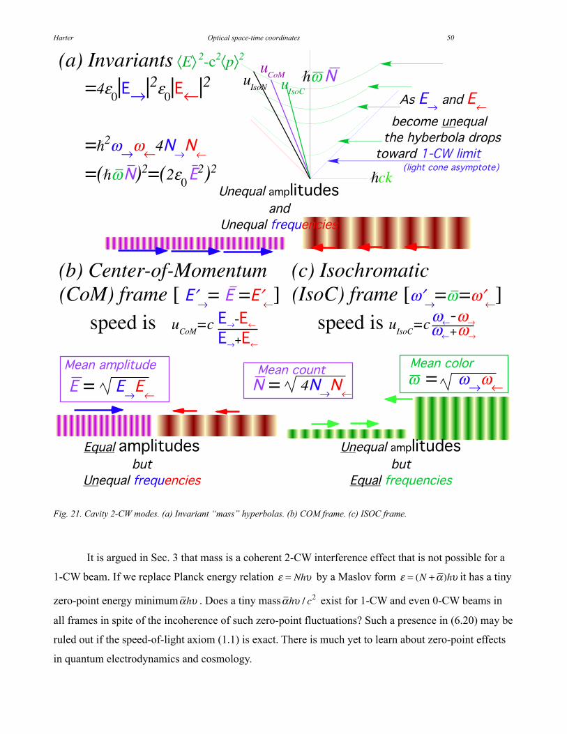
Harter Optical space-time coordinates 50
ω←-ω→ω←+ω→
(c) Isochromatic(IsoC) frame [ω′
→=ω =ω′
←]
speed is uIsoC
=c-→�-←
-→2-←
(a) Invariants ⟨E⟩ 2-c2⟨p⟩2
=4ε0|-→|2ε
0|-←|2
=h2ω→ω←43→3←
=(hω 3)2=(2ε0
-2)2hck
uCoMu
IsoNhω 3
������/��-→�$���-←��������(����4$����5��56�����$���'���7$����08��%(%�
ω = ω→ω←
#�$������
-�= -→-←
#�$��$('�%���
+��4$��$('�%����$��
+��4$����4���%��
(b) Center-of-Momentum(CoM) frame [ -′
→= -�=-′
←]
speed is uCoM
=c
-4$��$('�%������
+��4$����4���%��
+��4$��$('�%������
-4$����4���%��
3�= 43→3←
#�$������
uIsoC
��%�5�������$�6('����
Fig. 21. Cavity 2-CW modes. (a) Invariant “mass” hyperbolas. (b) COM frame. (c) ISOC frame.
It is argued in Sec. 3 that mass is a coherent 2-CW interference effect that is not possible for a
1-CW beam. If we replace Planck energy relation = Nh by a Maslov form = (N + )h it has a tiny
zero-point energy minimum h . Does a tiny mass h / c2 exist for 1-CW and even 0-CW beams in
all frames in spite of the incoherence of such zero-point fluctuations? Such a presence in (6.20) may be
ruled out if the speed-of-light axiom (1.1) is exact. There is much yet to learn about zero-point effects
in quantum electrodynamics and cosmology.

Harter Optical space-time coordinates 51
Photon-N vs Coherent- -states
Optical fields A or E have quantum expectation values of field operators based on mode amplitudes
ak or ak* in classical energy k
2ak*ak . Each ak or ak
* is replaced by oscillator boson operator ak or
ak
† in
a quantum field Hamiltonian H =
k(a
k†a
k+ ) whose eigenstates
N1N2 Nk have exact quantized
photon numbers
ak†ak = Nk for each mode-km.
Each mode phase quanta m and amplitude quanta Nm are invariant constants that define another
hyperbola with Einstein-Planck proper frequency
N ,m = Nm m as sketched in Fig. 21a and Fig. 22. The
problem is that absolute certainty of photon number Nm implies totally uncertain field phase just as
absolutely certain km of 1-CW symmetry implies totally uncertain position in space and time.
Space-time position coordinates were defined by taking 1-CW combinations to make 2-CW
coordinates of Fig. 3b, Fig. 6c, or Fig. 7c. Ultimately an n-CW pulse-wave (PW) of Fig. 2, Fig. 3a, Fig.
6d, or Fig. 7d was localized with as low a space-time uncertainty as desired but it acquires per-space
uncertainty or bandwidth according to Fourier-Heisenberg relation · >1.
So also must photon-number states be combined if amplitude and phase uncertainty are to be
reduced to the point where wave space-time coordinates can emerge. Such combinations are known as
coherent states or -states of harmonic oscillation. Sharper wave zeros require fuzzier hyperbolas.
Fuzzy hyperbolas vs. fuzzy coordinates
Model micro-laser states are coherent states =N N
N made of single-mode eigenstates
N = (a1
† )N 0 with amplitudes N=
Ne2 /2 / N ! . Variable = x + ip = ei is average mode phase, and
(x = Re , p = Im ) , rescaled by a quantum field factor f, are field averages
A , A = E( ) .
A = A = + *( ) f = + *( )2 0 V
(6.22)
Amplitude factor f makes Planck’s E = N equal Maxwell field energy E = U V .
U V = 2 0
2V A2=
2= N (6.23)
A fundamental laser mode in a 0.25μm cubic cavity (See E-wave sketched in one strip of Fig.
6c.) has green light with = 4 10 19 Joule or 2.5eV per photon. The average photon number
N =2= 1010 models a laser with mean energy
E = U V = N = 4.0 nanoJ in a volume V = (4
1 μm)3 .
Photon number uncertainty N = = 105 varies inversely to phase uncertainty = / 3 10 5 .
Amplitude expectation value N A N is zero for N states due to incoherence of phase, but
number value
N ak†a
kN = N is exact as is proper frequency N due to the phase factor (e i t )N of
(a1
† )N . A volume V with (N = 1010 ) -photons has energy E = N or mass-equivalent M = E / c2
= 10 25 kg
on a hyperbola 1010 quanta above the N=1 hyperbola. A coherent-state = 105 has a mass of about
M = 10 25 kg with uncertainty M = 10 30 kg so its phase uncertainty 3 10 5 is low enough to plot grids like
Fig. 6c or Fig. 23a. A low- state (Fig. 23c) has too few photon counts-per-grid to plot sharply. Photon
eigenstate N is a wash even for high-N since N = 0 has total (2 ) phase uncertainty. (Fig. 23d)

Harter Optical space-time coordinates 52
Fig. 22 Optical cavity energy hyperbolas for mode number n=1-3 and photon number N=0, 1, 2,....
(a) |α=105⟩ (b) |α=103⟩ (c) |α=101⟩ (d) |n=1010⟩Quantum field coherent α-states Photon number n-states
Fig. 23 Simulated spacetime photon counts for coherent (a-c) and photon-number states (d).

Harter Optical space-time coordinates 53
Deeper symmetry axioms
Discussion of relativity and quantum theory of wave amplitude requires further details. This
includes Dirac’s extraordinary theory that 2-CW light of certain frequencies in a vacuum may create
“real” matter that does not vanish when the light is turned off. For example, we know that two 0.51MeV
-ray photons of frequency e=mec2/ may create an electron and positron “hole” that form positronium
e + e pairs. Also, 0.94GeV -rays with p=mpc2/ may create proton-anti-proton p + p pairs, and so on.
Dirac creation processes raise questions, “What “cavity” traps 0.51MeV -pairs into stable e + e
pairs?” The discussion so far has only begun to define 2-CW symmetry properties by phase rates in
per-spacetime (K, )-quantum variables. Conservation (5.2) of these kinetic (K, )-values means that
the e + e or p + p pairs have the same (K, )-values as the 2-CW light that “creates” them, yet some other
less familiar internal lepton or baryon quantum variables may change as light becomes “trapped.” This
is beyond the scope of this discussion, and indeed, still largely beyond what is presently known.
7. Photo-emission
In the meantime it is fair to consider an electron, proton, or atom of mass M as having the same
kinetic symmetry as a 2-CW light beam of frequency =Mc2/ . This provides a simplified geometrical
construction for recoil shifts in atomic or nuclear 1-photon-emission, 1-photon-absorption, or 2-photon
Raman-Compton scattering processes by relating them to Doppler shifts on a (k, )-baseball diamond of
a virtual 2-CW photon symmetry hidden in any atom or particle.
Feynman recalls trying to answer his father’s question, “Where is a photon before an atom
emits it?” A pricey MIT education seemed not up to this question.27
Let us try to answer Feynman’s
father’s query in a quantitative way using a 2-CW photon model of an atom that emits some of its
“inner light” allowing a simpler Compton kinetics that uses the diamond geometry of Fig. 24.
Using the baseball diamonds of Fig. 6 or 7, we say atoms have the symmetry of 2-photon states
represented by 2nd
base K2 . In the lower half of Fig. 24a, a 1st base K1= ( , ) and 3
rd base K3= ( , )
sum to an atom’s 2nd
base K2= (0, 2 ) on a hyperbola of mass MQ at Q.
M
Q= 2 / c2 (7.1)
The pitcher’s mound P represents a 1-photon momentum-energy expectation value EP at Kp= (1 / 2)K2
E
P= / c2 (7.2)
It is like Fig. 10 or Fig. 12, but Q is a 2-photon state of energy MQ=2EP.
In Fig. 24a an emitted photon QP is imagined being “cut” from 3rd
base so 3 = shrinks by
what we will call28
a father-Feynman factor ff as 3rd
base alone loses the outgoing QP photon energy.
3 = ff = 3 QP (7.3)
If 1st base stays at its old value ( 1 = = 1 ) the 2
nd base moves from Q on its initial 2 -hyperbola to P
on its final 2 -hyperbola. Its new proper frequency is a geometric mean of 3rd
and 1st as in Fig. 10.

Harter Optical space-time coordinates 54
2 = 2 3 1 = 2 ff (7.4a) 3 = f = ff (7.4b) 1 = f 1= f 1 f = 1 (7.4c)
P
ωQ P
Q
O
P
ComptonScatteringProcesses
ωPQ
ωaxis
ck-axis
P
P
axis
2ω
Q P
Photo-Emission
Q
PωQP
P Q
Photo-Absorption
P
Q
ωPQ
Q
Q
O
R
S
axis
ωQP
ωPQ
1st base3rd base
ωQPQ
P
ωQP
9��9
Q
3rd base
2nd base2ω
ω K1K3
ωPQ
9'$���9ωPQ
P
P
Q
(a) (b)
(c)
1st base
(final)
ω1 = ω1
ω1 = ω
ω 3 = 41ω 3
2ω
ω 3 =ω 3ω1 = 4ω1
Q
M3
-hyperbola
M2-hyperbola
M1-hyperbola
P
Q
3ω
2ω
P
(initial)
recoilρ
recoilρ
(r1=M1c2/��)
NewtonKE2-circle
NewtonKE3-circle
(r2=M2c2/h�)
NewtonKE1-circle
P
O
h
4ϖ
3ϖ
2ϖ
ϖ
ϖ/2
Fig. 24 Optical cavity model of (a) Emission, (b) Absorption, and (c) Compton scattering
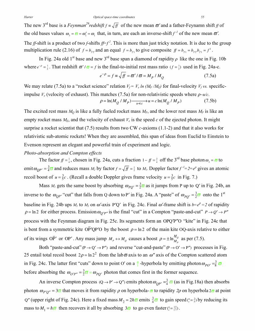
Harter Optical space-time coordinates 55
The new 3rd
base is a Feynman29
redshift f ff of the new mean and a father-Feynamn shift ff of
the old bases values 3 = = 1 = 1 that, in turn, are each an inverse-shift f -1 of the new mean .
The ff-shift is a product of two f-shifts ff=f 2. This is more than just tricky notation. It is due to the group
multiplication rule (2.16) of f = b3 2 and an equal f = b2 1 to give composite ff = b3 1 = b3 2 b2 1 = f 2 .
In Fig. 24a old 1st base and new 3
rd base span a diamond of rapidity like the one in Fig. 10b
where e =21 . That redshift / = f is the final-to-initial rest mass ratio ( f =
21) used in Fig. 24a-c.
e = f ff = / = MP / MQ (7.5a)
We may relate (7.5a) to a “rocket science” relation Vf = Ve ln (MF /ME) for final-velocity Vf vs. specific-
impulse Ve (velocity of exhaust). This matches (7.5a) for non-relativistic speeds where ~u/c.
= ln(MQ / MP )
u cu = c ln(MQ / MP ) (7.5b)
The excited rest mass MQ is like a fully fueled rocket mass MF, and the lower rest mass MP is like an
empty rocket mass ME, and the velocity of exhaust Ve is the speed c of the ejected photon. It might
surprise a rocket scientist that (7.5) results from two CW c-axioms (1.1-2) and that it also works for
relativistic sub-atomic rockets! When they are assembled, this span of ideas from Euclid to Einstein to
Evenson represent an elegant and powerful train of experiment and logic.
Photo-absorption and Compton effects
The factor ff = 41 , chosen in Fig. 24a, cuts a fraction 1 ff = 4
3 off the 3rd
base photon 3 = to
emit QP = 43 and reduces mass M2 by factor f = ff = 2
1 to M1. Doppler factor f -1=2=e gives an atomic
recoil boost of u = 53c . (Recall a double Doppler gives frame velocity u = 5
3c in Fig. 7.)
Mass M1 gets the same boost by absorbing PQ = 23 as it jumps from P up to Q in Fig. 24b, an
inverse to the QP “cut” that falls from Q down to P in Fig. 24a. A “paste” of PQ = 23 onto the 1
st
baseline in Fig. 24b ups M1 to M2 on -axis P Q in Fig. 24c. Final -frame shift is b=e =2 of rapidity
= ln 2 for either process. Emission Q P is the final “cut” in a Compton “paste-and-cut” P Q P
process with the Feynman diagram in Fig. 25c. Its segments form an OPQ P O “kite” in Fig. 24c that
is bent from a symmetric kite OP QP O by the boost = ln 2 of the main kite OQ-axis relative to either
of its wings OP or OP . Any mass jump MP
MQ causes a boost = ± ln
MP
MQ as per (7.5).
Both “paste-and-cut” (P Q P ) and reverse “cut-and-paste” (P O P ) processes in Fig.
25 entail total recoil boost 2 = ln 22 from the lab axis to an axis of the Compton scattered atom
in Fig. 24c. The latter first “cuts” down to point O on a 2 -hyperbola by emitting photon PO =83
before absorbing the O P = 23
= PQ photon that comes first in the former sequence.
An inverse Compton process (Q P Q ) emits photon QP =43 (as in Fig.18a) then absorbs
photon P Q = 3 that moves it from rapidity on hyperbola- to rapidity 2 on hyperbola 2 at point
Q (upper right of Fig. 24c). Here a fixed mass M2 = 2 emits 4
3 to gain speed (cu= 5
3) by reducing its
mass to M1 = then recovers it all by absorbing 3 to go even faster (c
u= 1 7
15) .

Harter Optical space-time coordinates 56
Photon K-vectors for any Compton process between 2:1-rest mass hyperbolas make a -warped
baseball diamond with =ln2 according to (7.5) as shown in Fig. 24c and Fig. 25a. Like a 2:1-Doppler
diamond in Fig. 10b, it has an aspect ratio that is twice its blue-shift b=e =2, that is 2e =4. Unlike the
basic diamond in Fig. 10b, the one in Fig. 25a is suspended on K-vectors of initial, intermediate, and
final atomic states that form the Feynman graphs in Fig. 25b-c. By drawing the vectors and graphs in
the center of momentum (COM) frame Fig. 25d-f, an original diamond like Fig. 6a-b is made.
A 2:1-rest mass drop shows geometry more clearly than a realistic ratio 1010
:1010
-1 for an atomic
transition that is about 10-10 of rest mass. Atomic rest-energy level ratios Em: Eh are close to unity and
fortunately so for our health! Harmonic levels with integral m:h ratios used in Fig. 24 apply to optical-
cavity models but m and h are small integers only for special spectra like Rydberg or rotor transitions.
P
Q
O
P
ωh
ωm
ωl
ωhsinh ρ
ωhcosh ρ
ωm =ωhe
−ρ
ωmsinh ρ
ωPQ = ωmh
ωO P = ωmh=ωhsinh ρ = ωPQ
P
Q
ωQP
P
P
O
ωP Q
ωm
ωl
ωmsinh ρωmsinh ρ
ωh
Q
P
P
ωQ P
ωPQ
O
P
ωP O
ωO P
P(b)�P O P ��:'$���
(a) Compton scattering geometry (c)�P Q P '$���:��
P
P
OωP Q
ωQP
P
Q
ωQP
PωP Q(e)� O P
�COM
P
(d) Center of momentum (COM) geometry
(f)� Q P �COM
P
ωP O = ωml= ωlsinh ρ = ωQ P
MEAN ωCOM
ωP Q =ωmsinh ρ=ωQP
ωQ P = ωml
ωml
INPUT ωIN photon
OUTPUT ωOUT photon
Fig. 25 Compton scattering. (a) Vector sums on mass hyperbolas of low , medium m , and high h. (b-c) Feynman
graphs. (d) Center of Momentum (COM) vector sums. (e-f) COM Feynman graphs.
Compton-Doppler staircase
In going from higher hyperbola h to middle m the lab recoil shift is fhm = e hm = hm by (7.5),
and its emitted frequency h m is the altitude of a kite triangle, like P QP in Fig. 24c, given as follows.
hm = (1 fhm2)
h
2=
h2 m2
2h= m sinh hm (7.6)
The example in Fig. 24a has QP = 43
= 2,1 . Doppler shifts of 2,1by f2,1 = 21 form a geometric series
( , 32
3 , 163 , 8
3, 43, 2
3, 3,6,12, ) of steps on a Compton staircase PQ P Q ... between (2:1)-levels 2 and1

Harter Optical space-time coordinates 57
in Fig. 24c. For any rational level ratio e hm = mh , each dilation factor
hm, recoil
hm, or ratio hm / is a
rational ratio, too, and the Pythagorean sum 1 =hm
2+
hm2 belongs to a rational triangle, e.g.,1 =
5232
+5242
.
hm =uhm
c= tanh hm =
h2 m2
h2+ m2
(7.7a)
hm = cosh hm =h2
+ m2
2mh(7.7b) sinh hm =
h2 m2
2mh(7.7c)
Recoil trims emitted hm below =|h-m| by a factor (h+m)/2h while absorption mh costs more than
by a factor (h+m)/2m. Newtonian recoil KEh
Mhu2 / 2 is a circle of radius M
hc2 in Fig. 24, so even low-u
recoil costs a little. Photons, like money-changing tourists, get nicked coming and going.
An absorption (m<h) frequency m h =IN is greater than emission h m by a factor fmh = m
h . A
Compton OUT due to IN is less than hm by the inverse factor fmh1= fhm = h
m . Hence a Compton
output OUT is less than its input IN by the Doppler ratio-square ff = fhm2
= ( hm )2 as shown before.
IN= mh = m
hhm , OUT
= hm
h m = ( hm )2 IN (7.8)
Compton processes in Fig. 25 start on middle m = m hyperbola to do a 2-photon bounce off a lower
= or a higher
h= h hyperbola. An intermediate “bouncer” is said to be a virtual level if its
or h values are integration variables being summed. A process (m h m) or (m m) is said to be
a resonant Compton process if an h-state or -state exists. Whether numbers m, h , and are integers in
a cavity model or real values for an atomic model, the results (7.6), (7.7), and (7.8) apply in any case.
Inverse frequencies
1= (kc) 1
= (2 c) 1 / c give the famous Compton wavelength sum rule.
( OUT ) 1= ( IN ) 1
+ 2(m ) 1 , or:
OUT=
IN+ 2 C where:
C =c
m=
M mc.
Compton radius C C / 2 is a minimum cavity radius with a frequency equal to the “zwitterbevegun”
of mass Mm. As input
IN reflects from an Mm-cavity it picks up diameter 2 C to become
OUT . Size
OUT
depends on mass Mm of level-m, not on Mh or M of higher level-h or lower level- that bounces level-m.
Compton radius is a curious measure of mass size. Larger mass M m has a smaller C
size that recoils
less and reflects photons elastically as one expects in classical wave optics where light is “light.”
A geometric f p -series
(… f 2 , f 1,1, f 1, f 2…) of levels also has a geometric series f p f 2 1
2 of
transitions. This gives Compton “nets” such as the ( f = 2) -net in Fig. 26a or a finer ( f = 2) -net in Fig.
26b. Finer fractions (f 1) give smaller jumps and acceleration that is more continuous and constant.
An acceleration of space-time frames by geometric or exponential frequency chirping is
described below. The space-time grids have a geometric spacing that is like the Compton nets in Fig.
26 below. The space-time grids are at right angles to the per-space-time nets to which they are
equivalent. They provide an optical realization of Einstein’s famous constant-g elevators.
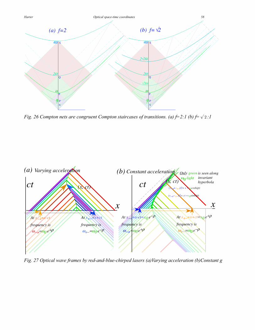
Harter Optical space-time coordinates 58
2ω
ω
4ω
Q
P
ω2
S
p
q
4ω
Q
P
S
p
q
2ω
2 2ω
ω
ω2
2ω
(a) f=2 (b) f= 24ω
Fig. 26 Compton nets are congruent Compton staircases of transitions. (a) f=2:1 (b) f= 2 :1
x
is seen along invariant hyperbola(x, ct)
(x→+x←)/2= x = x0 cosh(ρ)
(x→-x←)/2= ct = x0 sinh(ρ)
Only green ω0-light
ct
(b) Constant acceleration
At x←=x+ct= x0 e+ρ�
frequency is
ω← =ω0 e−ρ
At x→=x-ct= x0 e−ρ�
frequency is
ω→ =ω0 e+ρ
x
ct (x, ct)
(a) Varying acceleration
At x→=x-ct
frequency is
ω→ =ω0 e+ρ
At x←=x+ct
frequency is
ω← =ω0 e−ρ
Fig. 27 Optical wave frames by red-and-blue-chirped lasers (a)Varying acceleration (b)Constant g
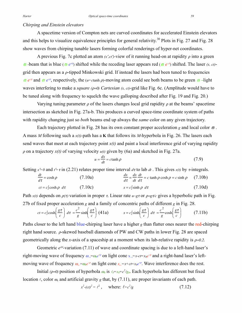
Harter Optical space-time coordinates 59
Chirping and Einstein elevators
A spacetime version of Compton nets are curved coordinates for accelerated Einstein elevators
and this helps to visualize equivalence principles for general relativity.30
Plots in Fig. 27 and Fig. 28
show waves from chirping tunable lasers forming colorful renderings of hyper-net coordinates.
A previous Fig. 7c plotted an atom (x ,ct )-view of it running head-on at rapidity into a green
-beam that is blue ( e+ ) shifted while the receding laser appears red ( e ) shifted. The laser (x, ct)-
grid then appears as a -tipped Minkowski grid. If instead the lasers had been tuned to frequencies
e and e+ , respectively, the (u=ctanh )-moving atom could see both beams to be green light
waves interfering to make a square ( =0) Cartesian (x, ct)-grid like Fig. 6c. (Amplitude would have to
be tuned along with frequency to squelch the wave galloping described after Fig. 19 and Fig. 20.)
Varying tuning parameter of the lasers changes local grid rapidity at the beams’ spacetime
intersection as sketched in Fig. 27a-b. This produces a curved space-time coordinate system of paths
with rapidity changing just so both beams end up always the same color on any given trajectory.
Each trajectory plotted in Fig. 28 has its own constant proper acceleration g and local color .
A mass M following such a x(t)-path has a K that follows its M-hyperbola in Fig. 26. The lasers each
send waves that meet at each trajectory point x(t) and paint a local interference grid of varying rapidity
on a trajectory x(t) of varying velocity u(t) given by (6a) and sketched in Fig. 27a.
u =dx
dt= ctanh (7.9)
Setting x =0 and t = in (2.21) relates proper time interval d to lab dt . This gives x(t) by -integrals.dt
d= cosh (7.10a)
dx
d=
dx
dt
dt
d= c tanh cosh = c sinh (7.10b)
ct = c cosh d (7.10c) x = c sinh d (7.10d)
Path x(t) depends on ( ) variation in proper . Linear rate u~g or =g /c gives a hyperbolic path in Fig.
27b of fixed proper acceleration g and a family of concentric paths of different g in Fig. 28.
ct = c coshg
c
d =
c2
gsinh
g
c
(41a) x = c sinh
g
c
d =
c 2
gcosh
g
c
(7.11b)
Paths closer to the left hand blue-chirping laser have a higher g than flatter ones nearer the red-chirping
right hand source. -skewed baseball diamonds of PW and CW paths in lower Fig. 28 are spaced
geometrically along the x-axis of a spaceship at a moment when its lab-relative rapidity is =0.2.
Geometric e± -variation (7.11) of wave and coordinate spacing is due to a left-hand laser’s
right-moving wave of frequency = 0e+ on light cone x =x-ct=x0e and a right-hand laser’s left-
moving wave of frequency = 0e on light cone x =x+ct=x0e+ . Wave interference does the rest.
Initial ( =0) position of hyperbola 0 is 0=x0=c2/g0. Each hyperbola has different but fixed
location , color , and artificial gravity g that, by (7.11), are proper invariants of each path.
x2-(ct)
2 =
2 , where: =c2/g (7.12)

Harter Optical space-time coordinates 60
l = 0.4
l = 0.4
Trailer has received 10 blue waves.
Trailer has received 5 blue waves.
Coherent waves make space-time coordinates of accelerating ship & trailer(s) for region inside asymptotic“event horizon”
Lab view ofLorentzcontractingseparation
Ship view ofinvariantproperseparationl = 0.4
Ship has received 5 green waves.
Geometrical Chirps Gives Accelerated Minkowski Grids
Ship has received 10 green waves.
Interfering light beams make Minkowski diamonds
Bouncing light Doppler shifts
from moving mirror .
BLUE- CHIRP spectrum results if mirror moves IN
RED- CHIRP spectrum results if mirror moves OUT
x or l-axis for rapidity r=0.2
TIME
TIME
Bouncing light Doppler shifts
from moving mirror .
Fig. 28 Accelerated reference frames and their trajectories painted by chirped coherent light
Frequency and acceleration g vary inversely with the path’s proper location relative to origin.
= c2/g = 0 c
2/g0 = const. (7.13)
Rapidity =g /c in (7.11) has proper time be a product of hyperbolic radius in (7.12) and “angle” .
c = c2/g = (7.14)
This is analogous to a familiar circular arc length formula s = r . Both have a singular center.
The less familiar hyperbolic center (x,ct)=(0,0) here begins an elementary event horizon. The
blue-chirp laser would need infinite frequency 0e+ at origin where ct=e goes to zero, so it gives up
before t=0. After t=0, light from the laser to any path S or T given by (7.11) never arrives. Fig. 28
shows paths of a spaceship S and a “trailer” T trailing by invariant length ST= (S)- (T) on an x-axis of
rapidity through origin (x,ct)=(0,0). S and T always have the same velocity (7.9) relative to the lab,
maintain proper interval ST , but trailer T feels greater g. Lower parts of a rigid rod accelerate more,
and this gives the lab-observed Lorentz length-contraction indicated at the top of Fig. 28.

Harter Optical space-time coordinates 61
In a Newtonian paradigm, asymmetric acceleration seems paradoxical, but if waves make a
coordinate frame, asymmetry is a consequence of the DeBroglie relation (3.5b) between k-vector and
momentum. Accelerating frames require shortening wavelength and this crowds waves.
Wave properties also manifest the accelerated frames’ upstairs-downstairs disparity in proper
time (“later” upstairs by (7.14)) and shift in frequency (lower or “red shifted” upstairs by (7.13)).
Along nodal (white) lines that are the ship-trailer x-axis for a momentary rapidity , wave phase is seen
to be some constant k = /2. The Einstein equivalence of gravity to an accelerated elevator is
manifested by a gravitational red shift and an increase of clock rates in the upstairs regions of a field.
A quantized version of Fig. 28 would be an atom with a transition at I, undergoing a sequential
resonant Compton scattering of exponentially chirped photons I, e±
I, e±2
I, e±3
I,… between the
same pair of hyperbolas in Fig. 28. The atom sees the same color and feels the same recoil rapidity at
each step in the quantum version of constant acceleration.
Constant velocity gives constant acceleration
This leads one to ask if chirped light might be used for atomic or molecular acceleration.
Logarithmic dependence =ln b of rapidity on Doppler b favors ultra-precise low energy acceleration,
more appropriate for nanotechnology than high energy acceleration with its extreme bandwidth.
The flip symmetry between two sides of a lightcone suggests optical cavities with a geometric
chirp. If you flip the diamond sequence in lower Fig. 28 across the light cone to the sides of Fig. 28
you get spacetime light paths bouncing between mirrors moving relative to each other. If mirrors close,
trapped light blue-chirps exponentially as on the right side in Fig. 28. It red-chirps if the two mirrors
separate as they do on the left side of Fig. 28. Together, a desired e±n
spectrum is made simply by
translating one etalon cavity at constant velocity relative to another stationary cavity that is enclosed
by the translating one.
In this way, light generated by mirrors of constant velocity provides the spectrum needed to
make an interference net of constant acceleration. Coherent acceleration like Fig. 28 (but slower)
might be done with great precision. Length metrology involves waves, too!
Wave geometry ought to make us more skeptical of the coordinate boxes and manifolds that
have been a paradigm for centuries. A common image is the Newton-Descartes empty-box at some
absolute time existing whether or not it contains any “particles.” Some learn to picture spacetime
coordinates as a giant metal frame of clocks like Fig. 9 in Taylor and Wheeler’s31
relativity text. That
figure is more like a parody of common views of spacetime manifolds that remain with us to this day.
Such a monstrosity of a framework is decidedly nonexistent and non-operational.
In contrast, a wave frame like Fig. 6, 7, and 22 is physical metrological coordinate system
whose geometry and logic is both revealing and real. The things being coordinated (waves) come with

Harter Optical space-time coordinates 62
their own coordinates and theorems built in. Einstein general theory of relativity trumped Newton’s
box by showing how it is affected (curved) by any energy or mass it holds. Quantum theory seems to
go a step further by indicating that this box and its contents may be one and the same thing.
Pair creation and quantum frames.
Dirac, before others, realized that per-spacetime has the symmetry of spacetime. Past and future
(time-reversal) symmetry demands negative frequency as well as positive. In order to visualize Dirac’s
pair-creation process he extends the playing field to back-to-back baseball-diamonds with four nets of
invariant hyperbolas. Examples of pair-creation are sketched in Fig. 29 as seen from two different
reference frames. Pair creation-destruction is then seen a strange sort of Compton process.
The Feynman graph of Compton scattering in Fig. 25c-d is turned on its side in Fig. 29 so it
may start and end on different branches of the m-hyperbola corresponding to mass ±m. Two photons,
whose energy sum equals the energy gap 2mc2, appear to bounce off intermediate hyperbolas in Fig. 29
that are conjugate hyperbolas defining group wavevectors Kg in Fig. 6 or 7. Such dispersion is said to
belong to instanton or tachyon waves of imaginary frequency ±i μ that entails a huge damping factor
emc2 / that proscribes their direct observation. They are said to be in the virtual or intermediate realm.
ck
ω
ck
-mc2/h
+mc2/h
Fig. 29 Dirac matter-antimatter dispersion relations and pair-creation-destruction processes.
Dirac’s is the first quantum theory to fully incorporate relativity. It introduces dual anti-worlds,
in which all three mass definitions (3.6), (3.7), and (3.9) have negative values, but leaves many
questions about their physical meaning. Analogies between the (2 e + e ) process in Fig. 29 and
exciton formation in the band theory of solids, shed some light on the physics. However, the exciton
process is a straight-up 1-photon process whose momentum is tiny compared to the energy jump, and it
lacks the world-anti-world symmetry of the Dirac exciton in which both the electron and an anti-
electron have the same group velocity but opposite momentum. The Dirac model has duality of
reversed energy (frequency), momentum (k-vector), space, and time that is quite extraordinary.
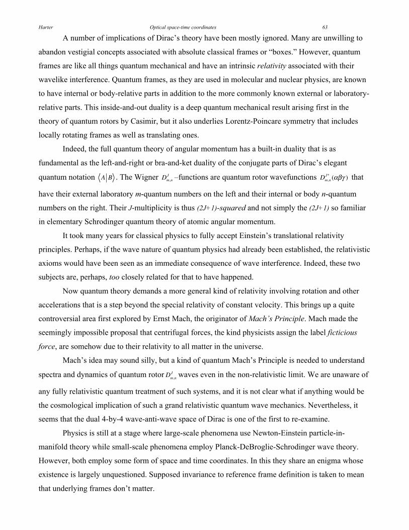
Harter Optical space-time coordinates 63
A number of implications of Dirac’s theory have been mostly ignored. Many are unwilling to
abandon vestigial concepts associated with absolute classical frames or “boxes.” However, quantum
frames are like all things quantum mechanical and have an intrinsic relativity associated with their
wavelike interference. Quantum frames, as they are used in molecular and nuclear physics, are known
to have internal or body-relative parts in addition to the more commonly known external or laboratory-
relative parts. This inside-and-out duality is a deep quantum mechanical result arising first in the
theory of quantum rotors by Casimir, but it also underlies Lorentz-Poincare symmetry that includes
locally rotating frames as well as translating ones.
Indeed, the full quantum theory of angular momentum has a built-in duality that is as
fundamental as the left-and-right or bra-and-ket duality of the conjugate parts of Dirac’s elegant
quantum notation A B . The Wigner Dm,nJ –functions are quantum rotor wavefunctions Dm,n
J* ( ) that
have their external laboratory m-quantum numbers on the left and their internal or body n-quantum
numbers on the right. Their J-multiplicity is thus (2J+1)-squared and not simply the (2J+1) so familiar
in elementary Schrodinger quantum theory of atomic angular momentum.
It took many years for classical physics to fully accept Einstein’s translational relativity
principles. Perhaps, if the wave nature of quantum physics had already been established, the relativistic
axioms would have been seen as an immediate consequence of wave interference. Indeed, these two
subjects are, perhaps, too closely related for that to have happened.
Now quantum theory demands a more general kind of relativity involving rotation and other
accelerations that is a step beyond the special relativity of constant velocity. This brings up a quite
controversial area first explored by Ernst Mach, the originator of Mach’s Principle. Mach made the
seemingly impossible proposal that centrifugal forces, the kind physicists assign the label ficticious
force, are somehow due to their relativity to all matter in the universe.
Mach’s idea may sound silly, but a kind of quantum Mach’s Principle is needed to understand
spectra and dynamics of quantum rotor Dm ,nJ waves even in the non-relativistic limit. We are unaware of
any fully relativistic quantum treatment of such systems, and it is not clear what if anything would be
the cosmological implication of such a grand relativistic quantum wave mechanics. Nevertheless, it
seems that the dual 4-by-4 wave-anti-wave space of Dirac is one of the first to re-examine.
Physics is still at a stage where large-scale phenomena use Newton-Einstein particle-in-
manifold theory while small-scale phenomena employ Planck-DeBroglie-Schrodinger wave theory.
However, both employ some form of space and time coordinates. In this they share an enigma whose
existence is largely unquestioned. Supposed invariance to reference frame definition is taken to mean
that underlying frames don’t matter.

Harter Optical space-time coordinates 64
That leaves our fundamental metrology in a dysfunctional dysphoria of an ignored spouse,
indispensable, but having only marginal identity. If Evenson and Einstein have taught us anything, it is
that this has to be a mistake. Frames do matter! The results of Dirac and many others have shown they
make matter and indeed are our matter.
References
1 K. M. Evenson, J.S. Wells, F.R. Peterson, B.L. Danielson, G.W. Day, R.L. Barger and J.L. Hall, Phys. Rev. Letters 29,1346(1972).2 Guinness Book of Records (1973).3 Glauber, Roy J., Hall, John L. and Hansch, Theodor W. The Nobel Prize in Physics, 2005. http://nobelprize.org/ 4 J. L. Hall and T. Hensch, Opt. Lett. 9, 502-504 (1984).5 N. Ashby, Physics Today, 55(5): 41 (May 2002).6 J. L. Hall, Laser Spectroscopy VII,(T. W. Hansch and Y. R. Shen, Eds., Springer-Verlag, 1985), pp. 393-394.7 William of Occam (1245-1326) “Pluralitas non est ponenda sine neccesitate” (Do not assume plurality withoutnecessity.)8 A. Cho, Science 306, 1461 (2004).9 A. Einstein, Annalen der Physik 17,891(1905). (Translation by W. Perrett and G.B. Jeffery, The Principle ofRelativity(with notes by A. Sommerfield) (Methuen, London 1923), (republished by Dover, London 1952).10 W. G. Harter, J. Mol. Spectrosc. 210, 166(2001).11 W. G. Harter, J. Evans, R. Vega, and S. Wilson, Am. J. Phys. 53, 671(1985).12 W.G. Harter and T. C. Reimer, //www.uark.edu/ua/pirelli/html/poincare_inv_2.htm13 D. E. Herschbach, (unpublished, 2005).14 H. Minkowski, Mathematisch-Physikalische Klasse, vol. 1, 53 (1908).15 H. A. Lorentz Koninklijke Akademie vanWetenschappen te Amsterdam. Section of Science. Proc. 6: 809-831 (1904).16 Albert Einstein "Zur Elektrodynamik bewegter Korper." Annalen der Physik 18,639 (1905); Annalen der Physik17,891(1905). (Translation: Perrett and Jeffery, The Principle of Relativity, (Methuen, London 1923), (Dover, 1952).17 Max Planck "Zur Theorie des Gesetzes der Energieverteilung im Normal-spectrum." Deutsche PhysikalischeGesellschaft. Verhandlungen 2: 237-245 (1900).18 Louis de Broglie, Nature 112, 540 (1923); Annalen der Physik (10) 2 (1923).19 P. A. M. Dirac, “Forms of Relativistic Dynamics” Rev. Mod. Physics, 21: 392 (1949).20 Albert Einstein "Uber einen die Erzeugung und Verwandlung des Lichtes betreffenden heuristischen Gesichtspunkt."Annalen der Physik 17: 132-148 (1905). (Translation by A.B. Aarons and M.B. Peppard, Am. J. Phys. 33, 367(1965).)21 E. Schrodinger, Annalen der Physik (4) 79 361 and 489 (1923); 80, 437 (1926); 81,109 (1926).22 Schrodinger’s protests about prevailing quantum mechanical interpretations are widely circulated. So far we have beenunable to locate more solid references.23 N. Bohr, Zeitschrift fur Physik, 9, 1-2, (1922).24 W. Heisenberg, The Physical Principles of the Quantum Theory, (Dover, New York, 1930).25 P.A.M. Dirac, Lectures on quantum mechanics, (New York, Belfer Graduate School of Science, Yeshiva University,
1964). Dirac’s first text in 1931 used and to denote bra-ket duality.26 A. Einstein, "I shall never believe that god plays dice with the universe" Albert Einstein Archives, The Jewish National &
University Library, The Hebrew University of Jerusalem (www.albert-einstein.org), Einstein Archives Online, Volume 15,
#294, Letter to Cornelius Lanczos, March 21, 1942,http://www.alberteinstein.info/db/ViewDetails.do?DocumentID=30893.27 R. Feynman, The Pleasure of Finding Things Out, (Perseus Publishing, Cambridge, MA,1999) p. 8.28 (unpublished) A huge energy shift is used for sake of geometric clarity. Atoms usually lose less than one part in 10
9 or
1010
of their rest mass in optical emission. The atom in the example loses rest mass 1/2 M2c2 emitting a 3/8 M2c
2 photon.
29 R. P. Feynman, R. Leighton, and M. Sands, The Feynman Lectures (Addison Wesley 1964) Our development owes a lot
to Feynman’s treatment cavity wave dispersion in Vol. II Ch. 24 and Vol. III Ch. 7.30 W. Rindler, Essential Relativity-Special, General, and Cosmological, Springer (New York 1977) p. 18. See also ref. 8, p.111.31 E.F.Taylor and J.A. Wheeler, Spacetime Physics (W. H. Freeman San Francisco 1966) p. 18.
AcknowledgementsThe author would like to thank Ronald F. Fox and Eric J. Heller for careful reading and suggestions regarding
early versions of this work and Daniel Kennefick for information from the Einstein Centennial bibliography
project. Also, we are grateful to Molly Longstreth and Usha Gupta for help with bibliographic search.

Harter Optical space-time coordinates 65
Figure CaptionsFig. 1. Comparison of wave archetypes and related axioms of relativity.
(a) Pulse Wave (PW) peaks locate where a wave is. Their speed is c for all observers.
(b) Continuous Wave (CW) zeros locate where it is not. Their speed is c for all colors (or observers.)
Fig. 2. Pulse Wave (PW) as a sum of 12 Fourier CW’s (a) PW parts: real Re , imaginary Im , and magnitude | |.
(b) CW phasor clocks plot real vs. imaginary parts of wave amplitude .
Fig. 3. Wave addition of counter propagating Fourier components.
(a) 2-PW Sum has binary sum has 4 values (0,0), (0,1), (1,0), (1,1) and diamond grid of peak paths on a plane of zeros.
(b) 2-CW Sum and interference has value continuum and square grid of zeros.
Fig. 4. “Ficticious” sources and their wave coordinate lattices in (a) Spacetime and (b) Per-spacetime.
CW lattices of phase-zero and group-node paths intermesh with PW lattices of “particle” or pulse wave paths.
Fig. 5. Co-propagating laser beams produce a collapsed wave lattice since all parts have same speed c.
Fig. 6. Laser lab view of 600Thz CW and PW light waves in per-space-time (a-b) and space-time (c-d).
Fig.7. Atom view of 600Thz CW and PW light waves in per-spacetime (a-b) and space-time (c-d) boosted to u=3c/5.
Fig. 8. Wave phasor addition. (a) Each phasor in a wave array is a sum (b) of two component phasors.
(c) In phasor-relative views either A or else B is fixed. An evolving sum-and-difference rectangle is
inscribed in the (dashed) circle of the phasor moving relative to the fixed one.
Fig. 9. Doppler shift b-matrix for a linear array of variously moving receiver-sources.
Fig. 10. (a) Euclidian mean geometry for counter-moving waves of frequency 1 and 4. (300THz units).
Fig. 10. (b) Geometry for the CW wave coordinate axes in Fig. 7.
Fig. 11. (a) Horizontal G-hyperbolas for proper frequency B=v and 2B and vertical P-hyperbolas for proper wavevector k.
(b) Tangents for G-curves are loci for P-curves, and vice-versa.
Fig. 12. Dispersion hyperbolas for 2-CW interference (a) Laser lab view. (b)Atom frame view.
Fig. 13. Geometry of contact transformation between relativistic (a) Hamiltonian (b) Lagrangian.
Fig. 14. “True” paths carry extreme phase and fastest phase clocks. Light-cone has only stopped clocks.
Fig. 15. Quantum waves interfere constructively on “True” path but mostly cancel elsewhere.
Fig. 16. Trigonometric geometry (a) Unit circular area =0.86. (b) Unit hyperbolic area =0.99.
Fig. 17. Relativistic wave mechanics geometry. (a) Overview. (b) Details of contact transform tangents.
Fig. 18. Monochromatic (1-frequency) 2-CW wave space-time patterns.
Fig. 19. Dichromatic (2-frequency) 2-CW wave space-time patterns.
Fig. 20. (a-g) Elliptic polarization ellipses relate to galloping waves in Fig. 18. (h-i) Kepler anomalies.
Fig. 21. Cavity 2-CW modes. (a) Invariant “mass” hyperbolas. (b) COM frame. (c) ISOC frame.
Fig. 22. Optical cavity energy hyperbolas for mode number n=1-3 and photon number Nn=0, 1, 2,....
Fig. 23. Simulated spacetime photon counts for coherent (a-c) and photon-number states (d).
Fig. 24. Optical cavity model of (a) Emission, (b) Absorption, and (c) Compton scattering
Fig. 25. Compton scattering. (a) Vector sums on mass hyperbolas of low , medium m , and high h.
(b-c) Feynman graphs. (d) Center of Momentum (COM) vector sums. (e-f) COM Feynman graphs.
Fig. 26. Compton nets are congruent Compton staircases of transitions. (a) f=2:1 (b) f= 2 :1.
Fig. 27. Optical wave frames by red-and-blue-chirped lasers (a)Varying acceleration (b)Constant g.
Fig. 28. Accelerated reference frames and their trajectories painted by e±
-chirped coherent light.
Fig. 29. Dirac matter-antimatter dispersion relations and diagrams of pair-creation-destruction processes.

Harter Optical space-time coordinates 66

Harter Optical space-time coordinates 67
-- The Purest Light and a Resonance Hero – Ken Evenson (1932-2002) --When travelers punch up their GPS coordinates they owe a debt of gratitude to an under sung
hero who, alongside his colleagues and students, often toiled 18 hour days deep inside a laser
laboratory lit only by the purest light in the universe.
Ken was an “Indiana Jones” of modern physics. While he may never have been called
“Montana Ken,” such a name would describe a real life hero from Bozeman, Montana, whose
extraordinary accomplishments in many ways surpass the fictional characters in cinematic thrillers like
Raiders of the Lost Arc.
Indeed, there were some exciting real life moments shared by his wife Vera, one together with
Ken in a canoe literally inches from the hundred-foot drop-off of Brazil’s largest waterfall. But, such
outdoor exploits, of which Ken had many, pale in the light of an in-the-lab brilliance and courage that
profoundly enriched the world.
Ken is one of few researchers and perhaps the only physicist to be twice listed in the Guinness
Book of Records. The listings are not for jungle exploits but for his lab’s highest frequency
measurement and for a speed of light determination that made c many times more precise due to his
lab’s pioneering work with John Hall in laser resonance and metrology†.
The meter-kilogram-second (mks) system of units underwent a redefinition largely because of
these efforts. Thereafter, the speed of light c was set to 299,792,458ms-1
. The meter was defined in
terms of c, instead of the other way around since his time precision had so far trumped that for
distance. Without such resonance precision, the Global Positioning System (GPS), the first large-scale
wave space-time coordinate system, would not be possible.
Ken’s courage and persistence at the Time and Frequency Division of the Boulder Laboratories
in the National Bureau of Standards (now the National Institute of Standards and Technology or NIST)
are legendary as are his railings against boneheaded administrators who seemed bent on thwarting his
best efforts. Undaunted, Ken’s lab painstakingly exploited the resonance properties of metal-insulator
diodes, and succeeded in literally counting the waves of near-infrared radiation and eventually visible
light itself.
Those who knew Ken miss him terribly. But, his indelible legacy resonates today as ultra-
precise atomic and molecular wave and pulse quantum optics continue to advance and provide
heretofore unimaginable capability. Our quality of life depends on their metrology through the Quality
and Finesse of the resonant oscillators that are the heartbeats of our technology.
Before being taken by Lou Gehrig’s disease, Ken began ultra-precise laser spectroscopy of
unusual molecules such as HO2, the radical cousin of the more common H2O. Like Ken, such radical
molecules affect us as much or more than better known ones. But also like Ken, they toil in obscurity,
illuminated only by the purest light in the universe.
In 2005 the Nobel Prize in physics was awarded to Glauber, Hall, and Hensch††
for laser optics
and metrology.
† K. M. Evenson, J.S. Wells, F.R. Peterson, B.L. Danielson, G.W. Day, R.L. Barger and J.L. Hall,
Phys. Rev. Letters 29, 1346(1972).
†† The Nobel Prize in Physics, 2005. http://nobelprize.org/
hysics, 2005. http://nobelprize.org/

Harter Optical space-time coordinates 68
Kenneth M. Evenson – 1932-2002