optical and magnetical properties of endohedral silicon cages · de gaiolas endoh edricas de sil...
TRANSCRIPT

Optical and Magnetical
Properties of Endohedral Silicon
Cages
Mario Rui Goncalves Marques
Department of Physics
University of Coimbra
Thesis Advisors:
Fernando Manuel da Silva Nogueira
Micael Jose Tourdot de Oliveira
A thesis submitted for the degree of
Master of Science
Coimbra, 14th July, 2015


I would like to dedicate this thesis to my loving parents ...

Acknowledgements
I would like to start thanking my supervisors, Dr. Fernando Nogueira
and Dr. Micael Oliveira, for all the help and lessons they gave me. I
learnt a lot.
I would like to thank my parents, I would not be here if not for them.
To my mother for the amazing stories. To my father, all that page
skipping sharpened my mind.
I would like to thank my favourite brother.
I would like to thank all my friends at the Physics Department.
Also, I would like to thank all the members of the Center for Compu-
tational Physics.
I would like to thank Maxwell-Boltzmann for their inspiration.
Finally, I would like to thank Blue for being there for me.

Abstract
This work shows a study of optical and magnetical properties of endo-
hedral silicon cages containing transition metal atoms. Geometries
with different magnetizations are calculated using density functional
theory and the optical response of these systems is obtained by em-
ploying real-time, real-space time-dependent density functional the-
ory. A comparison and discussion of the results is also present.

Resumo
Este trabalho mostra um estudo de propriedades opticas e magneticas
de gaiolas endohedricas de silıcio contendo atomos de metais de tran-
sicao. Geometrias para diferentes magnetizacoes sao calculadas usan-
do a teoria dos funcionais da densidade enquanto que a resposta optica
destes sistemas e obtida usando a teoria dos funcionais da densidade
dependente do tempo em espaco real e em tempo real. Uma com-
paracao e discussao dos resultados tambem e apresentada.

Contents
Contents vi
List of Figures x
List of Tables xii
I Introduction 1
II Theory 5
1 The Many Body Problem 7
1.1 A look into Many-Body theory . . . . . . . . . . . . . . . . . . . . 7
1.2 Interactions of electrons and nuclei . . . . . . . . . . . . . . . . . 8
1.2.1 Schrodinger equation . . . . . . . . . . . . . . . . . . . . . 9
1.2.2 Born-Oppenheimer Approximation . . . . . . . . . . . . . 10
1.3 The Rayleigh-Ritz principle . . . . . . . . . . . . . . . . . . . . . 12
1.4 Hellmann-Feynman Theorem . . . . . . . . . . . . . . . . . . . . . 13
2 Density Functional Theory 15
2.1 A look into DFT . . . . . . . . . . . . . . . . . . . . . . . . . . . 15
2.2 Hohenberg-Kohn Theorems . . . . . . . . . . . . . . . . . . . . . 16
2.3 Kohn-Sham Ansatz . . . . . . . . . . . . . . . . . . . . . . . . . . 21
2.4 Kohn-Sham Equations and Eigenvalues . . . . . . . . . . . . . . . 24
2.4.1 Spin Density Form . . . . . . . . . . . . . . . . . . . . . . 25
2.4.2 Relativistic Density Form . . . . . . . . . . . . . . . . . . 26
2.5 Exchange and Correlation Functionals . . . . . . . . . . . . . . . 27
vi
CONTENTS
2.5.1 Local Density Approximation . . . . . . . . . . . . . . . . 27
2.5.2 Generalized gradient approximation . . . . . . . . . . . . . 28
2.5.2.1 PBE . . . . . . . . . . . . . . . . . . . . . . . . . 28
3 Time Dependent Density Functional Theory 31
3.1 A look into TDDFT . . . . . . . . . . . . . . . . . . . . . . . . . 31
3.2 Runge-Gross Theorem . . . . . . . . . . . . . . . . . . . . . . . . 31
3.3 Time-Dependent Kohn-Sham Equations . . . . . . . . . . . . . . 35
3.4 Adiabatic Approximation for Functionals . . . . . . . . . . . . . . 37
3.5 Response Functions . . . . . . . . . . . . . . . . . . . . . . . . . . 38
3.5.1 Linear Response and Photo-absorption Spectra . . . . . . 39
3.5.2 Kohn-Sham Linear Response . . . . . . . . . . . . . . . . . 42
3.5.3 Time-Propagation Method . . . . . . . . . . . . . . . . . . 44
III Numerical Aspects 47
4 Pseudopotential Approximation 49
4.1 A look into Pseudopotentials . . . . . . . . . . . . . . . . . . . . . 49
4.2 Phillips and Kleinman Formal Construction . . . . . . . . . . . . 50
4.3 Norm-conserving Ab-Initio Pseudopotentials . . . . . . . . . . . . 51
5 The Projector Augmented Waves Method 55
5.1 A look into the PAW Method . . . . . . . . . . . . . . . . . . . . 55
5.2 Formalism . . . . . . . . . . . . . . . . . . . . . . . . . . . . . . . 56
5.2.1 Transformation operator . . . . . . . . . . . . . . . . . . . 56
5.2.2 Operators . . . . . . . . . . . . . . . . . . . . . . . . . . . 57
5.2.3 Total energy . . . . . . . . . . . . . . . . . . . . . . . . . . 59
5.3 PAW Method practical scheme . . . . . . . . . . . . . . . . . . . . 60
5.3.1 Overlap Operator . . . . . . . . . . . . . . . . . . . . . . . 60
5.3.2 Kohn-Sham Equations . . . . . . . . . . . . . . . . . . . . 61
5.3.3 Forces . . . . . . . . . . . . . . . . . . . . . . . . . . . . . 62
vii

CONTENTS
IV Applications 63
6 Methodology 65
6.1 Optical and Magnetical Properties . . . . . . . . . . . . . . . . . 65
6.2 Geometry optimization with ABINIT . . . . . . . . . . . . . . . . 66
6.2.1 A look into ABINIT . . . . . . . . . . . . . . . . . . . . . 66
6.2.2 PAW Method . . . . . . . . . . . . . . . . . . . . . . . . . 67
6.2.3 Geometry Optimization . . . . . . . . . . . . . . . . . . . 68
6.3 Photo-absorpion Spectra with Octopus . . . . . . . . . . . . . . . 68
6.3.1 A look into Octopus . . . . . . . . . . . . . . . . . . . . . 68
6.3.2 Pseudopotentials and APE . . . . . . . . . . . . . . . . . . 69
6.3.3 Photo-absorption Spectra . . . . . . . . . . . . . . . . . . 69
6.4 Overall Procedure . . . . . . . . . . . . . . . . . . . . . . . . . . . 70
7 Silicon cages with one transition metal atom 73
7.1 Results and discussion . . . . . . . . . . . . . . . . . . . . . . . . 73
7.1.1 Optimized geometries . . . . . . . . . . . . . . . . . . . . . 73
7.1.2 Photo-absorption Spectra . . . . . . . . . . . . . . . . . . 79
8 Silicon cages with two transition metal atoms 85
8.1 Results and Discussion . . . . . . . . . . . . . . . . . . . . . . . . 85
V Conclusion 87
References 91
viii

List of Figures
2.1 Schematic representation of the Hohenberg-Kohn Theorem. Start-
ing with the potential and going down, the solution of the Schrodinger
equation with the potential Vext(r) determines all states of the sys-
tem Ψi(r), including the state with lesser energy, the ground
state Ψ0(r) with density n0(r). The long arrow labelled HK
connects the ground state density with the external potential. . . 16
2.2 Schematic representation of the Kohn-Sham Ansatz. The left
scheme shows the schematic representation of Hohenberg-Kohn
theorem for interacting electrons while the right one shows the
same but for non-interacting electrons. The ansatz connects both
ground state densities. . . . . . . . . . . . . . . . . . . . . . . . . 21
2.3 Flow chart depicting the Kohn-Sham SCF cycle. . . . . . . . . . . 25
5.1 The All-electron PAW wavefunction as a sum of the pseudo wave-
function with the atomic partial wavefunction subtracted by the
partial pseudo wavefunction. . . . . . . . . . . . . . . . . . . . . . 56
7.1 Optimized geometries for the cages encapsulating a group four
transition metal atom. . . . . . . . . . . . . . . . . . . . . . . . . 74
7.2 Optimized geometries for the cages encapsulating a group five tran-
sition metal atom. . . . . . . . . . . . . . . . . . . . . . . . . . . . 75
7.3 Optimized geometries for the cages encapsulating a group six tran-
sition metal atom. . . . . . . . . . . . . . . . . . . . . . . . . . . . 75
7.4 Optimized geometries for the cages encapsulating a group seven
transition metal atom . . . . . . . . . . . . . . . . . . . . . . . . . 76
x

LIST OF FIGURES
7.5 Optimized geometries for the cages encapsulating a group nine
transition metal atom. . . . . . . . . . . . . . . . . . . . . . . . . 77
7.6 Optimized geometries for the cages encapsulating a group nine
transition metal atom. . . . . . . . . . . . . . . . . . . . . . . . . 77
7.7 Optimized geometries for the cages encapsulating a group ten or
eleven transition metal atom. . . . . . . . . . . . . . . . . . . . . 78
7.8 Photo-absorption spectrum for the endohedral silicon cages con-
taining one atom of Cr, Mn, Fe and Co for two different magneti-
zations. . . . . . . . . . . . . . . . . . . . . . . . . . . . . . . . . 79
7.9 Photo-absorption Spectra for CrSi12. Obtained using the default
LDA from octopus and the PBE (GGA). . . . . . . . . . . . . . . 80
8.1 Endohedral silicon cage with two transition metal atoms inside.
These structures have a D5h symmetry. . . . . . . . . . . . . . . . 85
8.2 Comparison between the Fe2Si15 and FeSi12 photo-absorption spec-
tra. The highest occupied molecular orbital eigenvalue is -4.90 eV. 86
xi

List of Tables
7.1 Some properties of the geometries presented in figure 7.1 . . . . . 74
7.2 Some properties of the geometries presented in figure 7.2. . . . . . 75
7.3 Some properties of the geometries presented in figure 7.3. . . . . . 76
7.4 Some properties of the geometries presented in figure 7.4. . . . . . 76
7.5 Some properties of the geometries presented in figure 7.5. . . . . . 77
7.6 Some properties of the geometries presented in figure 7.6. . . . . . 78
7.7 Some properties of the geometries presented in figure 7.7. . . . . . 78
7.8 Ionization potentials for the Cr, Mn, Fe and Co endohedral silicon
cages. . . . . . . . . . . . . . . . . . . . . . . . . . . . . . . . . . 80
7.9 Predominant peaks for the Cr, Mn, Fe and Co endohedral silicon
cages. . . . . . . . . . . . . . . . . . . . . . . . . . . . . . . . . . 82
xii

LIST OF TABLES
1

Part I
Introduction


Introduction
Until 1988’s discovery of the giant magnetoresistive effect, the spin of the
electron was completely ignored in electronic devices, based on electrons’ charge.
Currently, spintronics (spin based electronics) presents itself as an active field of
work, which exhaustively seeks new methods and models with the intent of creat-
ing spintronic devices in the near future. The advantages of these devices would
be nonvolatility, increased data processing speed, decreased electrical power con-
sumption and increased integration densities compared with conventional semi-
conductor devices [1]. One of the ideas that lay around is the possibility to control
the spin of a system using electric fields, since the spin-orbit interaction connects
the charge and spin dynamics of a system [2, 3]. In fact, this thesis is a contin-
uation of the work done in [3]. Imagine a building block that could be in any
of two stable states, each characterised by a different magnetization and let an
electrical field be able to change one state to the other. If each magnetization
state is associated with one number, 0 or 1, this could be the building block of
an hard disk.
The main objective of this work is to find endohedral silicon cages with differ-
ent structures, due to a different magnetization of the system and then, investigate
if these different structures can be identified by their photo-absorption spectrum.
Here endohedral is used based on its etymology, meaning there is something in-
side the structure, in this case, an atom, a molecule or a cluster of a transition
metal inside the silicon cage. To achieve a solution of this many-body problem
density functional theory (DFT) and time-dependent density functional theory
(TDDFT) will be used. While DFT permits to describe the ground state prop-
erties of the system, TDDFT shows ways to look into excited state properties
and provides response functions. These exact theories, which use the density as
Introduction
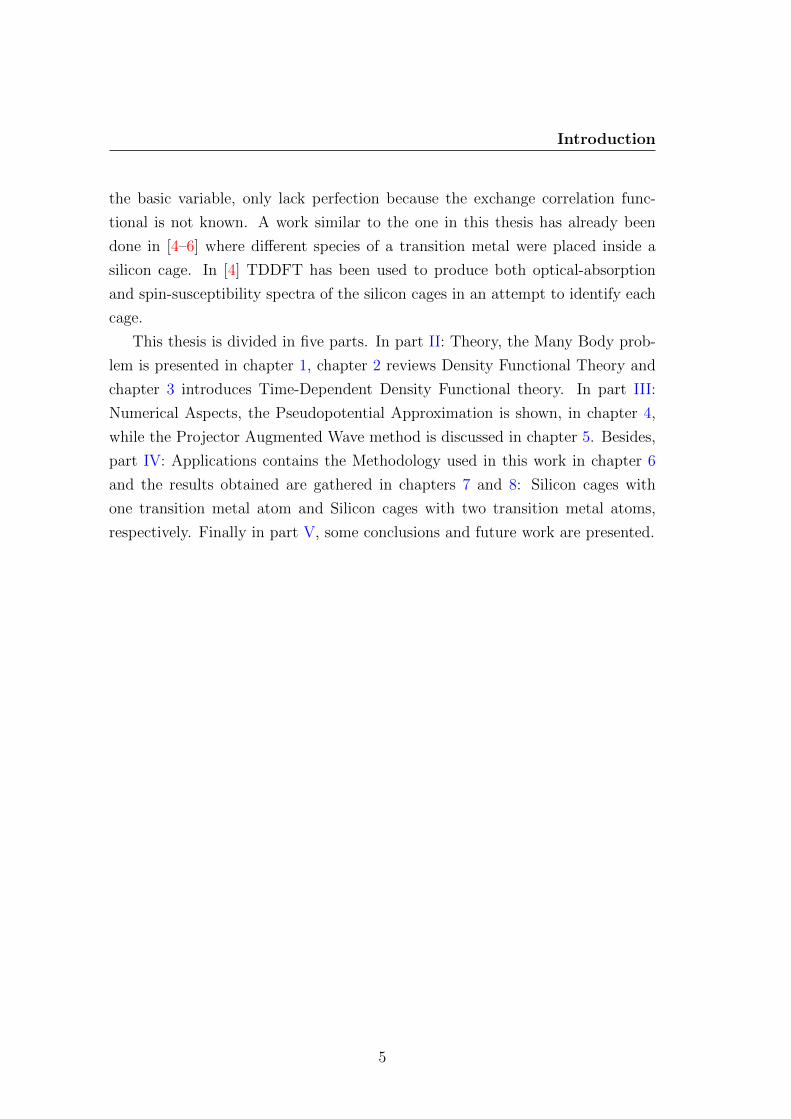
the basic variable, only lack perfection because the exchange correlation func-
tional is not known. A work similar to the one in this thesis has already been
done in [4–6] where different species of a transition metal were placed inside a
silicon cage. In [4] TDDFT has been used to produce both optical-absorption
and spin-susceptibility spectra of the silicon cages in an attempt to identify each
cage.
This thesis is divided in five parts. In part II: Theory, the Many Body prob-
lem is presented in chapter 1, chapter 2 reviews Density Functional Theory and
chapter 3 introduces Time-Dependent Density Functional theory. In part III:
Numerical Aspects, the Pseudopotential Approximation is shown, in chapter 4,
while the Projector Augmented Wave method is discussed in chapter 5. Besides,
part IV: Applications contains the Methodology used in this work in chapter 6
and the results obtained are gathered in chapters 7 and 8: Silicon cages with
one transition metal atom and Silicon cages with two transition metal atoms,
respectively. Finally in part V, some conclusions and future work are presented.
5

Part II
Theory


Chapter 1
The Many Body Problem
There are mysteries which men can only guess at, which age by age they may
solve only in part.
Bram Stoker
1.1 A look into Many-Body theory
Mysteries... The Many-Body problem [7, 8] shows perfectly how both com-
plicated and unrewarding physics can be. Think of an atom, or a molecule, placed
in any region of space and time, subject to whichever field, or fields, and basically
try to name all the interactions that maintain its structure and keep the electrons
bound to the nuclei, or not, if the field is strong enough... Now disregard almost
all of them, except for the interactions between electrons and nuclei and their
self interactions. Oh, and electrons and nuclei can move, but not very fast. One
should try to avoid those relativistic shenanigans as much as possible. This is the
many-body problem. Now, try to solve it. The peculiarity of this problem is that,
even after so much simplifications, it remains rather unsolvable... Strangely this
is what motivates physicists the most. The joy of the challenge, that dwell within
every phenomena exhibited by matter. Not only that, but the elegance of nature,
hidden behind the mysteries of the universe, and unveiled by that undoubtedly
extraordinary approach. It is quite remarkable.

1. The Many Body Problem
Also, further clarification should be made, about something that may, or may
not, have been written somewhere, relativity is awesome! And indispensable.
1.2 Interactions of electrons and nuclei
The Hamiltonian for a system of N electrons and M nuclei can be written as
H(r1, ..., rN ,R1, ...,RM) = −1
2
N∑i=1
∇2i −
N,M∑i,I=1
ZI|ri −RI |
+
+1
2
N∑i,j=1i 6=j
1
|ri − rj|−
M∑I=1
1
2mI
∇2I +
1
2
M∑I,J=1I 6=J
ZIZJ|RI −RJ |
,
(1.1)
where the lower case subscripts denote electrons at position ri and the upper case
subscripts denote nuclei at position RI . Here and throughout this thesis Hartree
atomic units are use. These units arise from casting the Schrodinger equation in
a dimensionless form as well as defining
e = me = ~ = 4πε0 = 1. (1.2)
In the last equation e stands for electron charge, me for electron mass, ~ for the
Planck’s constant and ε0 for the electric permeability of vacuum. In this unit
system length is given in bohr (1 a0 = 4πε0~mee2
= 0.5292 A), and energy in hartree
(1 Ha = e2
4πε0a0= 27.211 eV), the speed of light is c ' 137, the unit of time is
~Ha
= 2.419× 10⁻¹⁷ s, and the unit of force is Haa0
= 8.24× 10⁻⁸ N.
The first term of the aforementioned Hamiltonian is the kinetic energy operator
for electrons,
T = −1
2
N∑i=1
∇2i , (1.3)
while the second term, the potential operator, represents the interaction between
9

1. The Many Body Problem
electrons and nuclei,
V =
N,M∑i,I=1
v(ri,RI),= −N,M∑i,I=1
ZI|ri −RI |
, (1.4)
and the third, is the electron-electron interaction operator,
W =1
2
N∑i 6=j
1
|ri − rj|. (1.5)
The last two terms are the nuclei kinetic operator and the nuclei-nuclei interaction
operator
TN = − 1
2mI
M∑I=1
∇2I , WN =
1
2
M∑I 6=J
1
|RI −RJ |. (1.6)
1.2.1 Schrodinger equation
The fundamental equation governing a non-relativistic quantum system is the
time dependent Schrodinger equation,
i∂
∂tΨ(r, R, t) = H(r, R)Ψ(r, R, t). (1.7)
The abbreviation r = (r1, ..., rN) was used, as well as ri ≡ (r′i, σi), that is
the many-body wavefunction is a function of 3(N + M) spacial coordinates and
N +M spin coordinates.
As the Hamiltonian (1.1) is time-independent, the eigenstates of (1.7) can be
written as Ψ(r, R, t) = Ψ(r, R)e−iEt, where Ψ(r, R) is the solution
of the time-independent Schrodinger equation,
H(r, R)Ψ(r, R) = EΨ(r, R). (1.8)
Alas, this equation is normally impossible to solve.
10

1. The Many Body Problem
1.2.2 Born-Oppenheimer Approximation
Inspection of the many-body Hamiltonian provides a clue towards the simplifica-
tion of the many-body problem: the only small parameter is the inverse nuclear
mass, i.e. the nuclear kinetic energy term. As the electrons’ mass is smaller than
the mass of the nuclei, when the nuclei move, the electrons appear to adjust their
positions instantaneously. Therefore, the electrons move adiabatically with the
nuclei. This motivates the description of each nuclei as a point like static charge
and is the reasoning behind the adiabatic or Born-Oppenheimer approximation
[3, 7, 9]. Let the eigenvalues and the eigenfunctions for the electrons Ei(R) and
Ψi(r : R), which depend upon the nuclear positions as parameters, be the
solution of
H ′(r, R)Ψi(r : R) = EiΨi(r : R), (1.9)
where the electron Hamiltonian is given by
H ′(r, R) = T + W + V . (1.10)
As electrons obey Pauli’s exclusion Principle, this electron, many-body, wave-
function Ψi(r : R) must be antisymmetric with respect to the interchange of
any two electrons. Let Pij be an exchange operator that permutes the coordinates
of the electrons i and j:
PijΨi(r1, ..., ri, ..., rj, ...rN : R) = −Ψi(r1, ..., rj, ..., ri, ...rN : R). (1.11)
Since the electrons are indistinguishable, the new wavefunction and any other
wavefunctions created by application of the exchange operator are also eigen-
functions of the Hamiltonian (1.10).
The full solution for the coupled system (1.8) can be written in terms of Ψi(r :
R) because this wavefunction defines a complete set of states for the electrons
at each R. Therefore,
Ψ(r, R) =∑i
ξi(R)Ψi(r : R). (1.12)
11

1. The Many Body Problem
In the pursuit of decoupled equations for electrons and nuclei, one has to insert the
previous expansion in (1.8), multiply the expression on the left by Ψ†i (r : R)and integrate over the electron variables in order to obtain the equations for
ξi(R):
[TN +WN(R)+Ei(R)
]ξi(R)+
∑i
Cii′(R)ξi(R) = Eξi(R), (1.13)
with Cii′(R) =[Aii′(R) +Bii′(R)
]and
Aii′(R) =∑J
1
mJ
∫d3rΨ†i (r : R)∇JΨi′(r : R)∇J ,
Bii′(R) =∑J
1
2mJ
∫d3rΨ†i (r : R)∇2
JΨi′(r : R).(1.14)
At last, the only thing left in order to decouple the equations are the off-diagonal
terms Cii′ , sinceAii(R) = 0 from the normalization condition, whereasBii(R)can be added to WN(R) to determine a modified potential function for the nu-
clei Ui(R) = WN(R + Bii(R). The Born-Oppenheimer approximation
consists in neglecting those terms, i.e., the electrons are assumed to remain in
a given state k as the nuclei move. Although the electron wave function and
the energy of the state k change, no energy is transferred between the nuclear
degrees of freedom and the excitations of the electrons. This approximation is
rather good and only presents problems when degeneracies of the electronic states
make the off-diagonal terms become large. Thus, the decoupled equations can be
written as
T + W + V (r, R)Ψi(r : R) = Ei Ψi(r : R)
TN + Ui(R) + Ei(R) ξi(R) = E ξi(R).(1.15)
In spite of the simplifications that arose from the adiabatic approximation, these
equations are far too difficult to solve for a reasonable number of electrons and
nuclei. Normally, in electronic structure, the equation for the nuclei is neglected in
favour of a classical one while the equation for the electrons is further simplified.
12

1. The Many Body Problem
From this point forward, the dependency of the electron wavefunctions with the
nuclear coordinate will be omitted from the equations for simplicity.
1.3 The Rayleigh-Ritz principle
Before attempting to solve the first equation of (2.2), it is important to under-
stand the Variational or Rayleigh-Ritz principle [10].
The average of many measurements of the energy of a system in state Ψ can be
written as a functional of that state:
E[Ψ] =〈Ψ| H |Ψ〉〈Ψ|Ψ〉
. (1.16)
Furthermore, since each measurement of the energy provides one of the eigenval-
ues of H, the energy calculated from a guess Ψ has to be an upper bound to the
ground state energy E0
E0 ≤ E[Ψ]. (1.17)
This can be easily proven by insertion of Ψ =∑
iCiΨi in the energy functional
E[Ψ] =
∑i |Ci|2Ei∑i |Ci|2
. (1.18)
As E0 ≤ E1 ≤ E2 ≤ ..., the minimum of the energy functional is only reached
when Ψ = C0Ψ0.
Therefore, the ground state energy can be found by minimization of the energy
functional with respect to all allowed N electron wave functions
E0 = E[Ψ0] = minΨE[Ψ]. (1.19)
Consequently, the variation of the energy functional with respect to the wave
function has to be stationary for the ground state, that is
δE[Ψ0]
δΨ∗0=
HΨ0
〈Ψ0|Ψ0〉− 〈Ψ0| H |Ψ0〉Ψ0
〈Ψ0|Ψ0〉2= 0 hence HΨ0 = E0Ψ0. (1.20)
13

1. The Many Body Problem
In fact, all eigenstates are stationary points, therefore the Schrodinger equation
can be written as
δ[〈Ψ| H |Ψ〉 − E(〈Ψ|Ψ〉 − 1)] = 0, (1.21)
where E is the Lagrange multiplier.
1.4 Hellmann-Feynman Theorem
In classical mechanics, given a Hamiltonian HRIdepending on the parameter RI ,
one can define a force F = − ∂H∂RI
which is associated with the parameter in the
sense that F dRI is the work done in changing the parameter by dRI . In Quantum
Mechanics there are, in principle, two ways of calculating said force: F = − ∂Ei∂RI
,
where Ei(RI) are the eigenvalues of state Ψi, or as F = −〈Ψi| ∂H∂RI|Ψi〉. The
Hellmann-Feynman theorem ensures that both definitions are equivalent [11].
Derivation of the energy functional with respect to the nuclear coordinates, and
assuming 〈Ψ|Ψ〉 = 1 for convenience, leads to
∂E
∂RI
= 〈Ψ| ∂H∂RI
|Ψ〉 + 〈 ∂Ψ
∂RI
|H|Ψ〉 + 〈Ψ|H| ∂Ψ
∂RI
〉 . (1.22)
If the Hamiltonian is an Hermitian Operator and has eigenvalues Ei
∂E
∂RI
= 〈Ψ| ∂H∂RI
|Ψ〉 +∑i
|Ci|2Ei∂
∂RI
〈Ψi|Ψi〉 . (1.23)
Then, conservative forces can be calculated as
FRI= − ∂E
∂RI
= −〈Ψ| ∂H∂RI
|Ψ〉 = −〈Ψ| ∂
∂RI
[V + WN
]|Ψ〉 . (1.24)
14

1. The Many Body Problem
15

Chapter 2
Density Functional Theory
No great discovery was ever made without a bold guess.
Isaac Newton
2.1 A look into DFT
Guess... Currently, Density Functional Theory [10, 12, 13] provides the
most popular methods used in electronic structure. This theory as become so
widespread because it provides both accurate and swift results for many proper-
ties of atoms, solids and molecules. Simulations using DFT have discovered new
materials and predicted many physical phenomena.
The success of this theory is related with the replacement of the wavefunction
with the ground state density as the basic variable, therefore allowing to express
all quantum mechanical observables as a functional of a real scalar function of
three variables. This may not look like a big deal, but the storage space needed,
when performing calculations with the wavefunction as the basic variable, scales
with M3N , where n is the number of electrons, the 3 accounts for the spacial
coordinates and M for the mesh points (neglecting spin).
Another outstanding guess, partially responsible for the triumph of DFT was
the replacement of a problem of interacting electrons by the problem of non-
interacting particles under a peculiar potential.

2. Density Functional Theory
2.2 Hohenberg-Kohn Theorems
The approach of Hohenberg-Kohn [14] consists in the formulation of Density
Functional Theory as an exact theory of many body systems. The foundations
of DFT consists in two theorems named after Hohenberg and Kohn.
Figure 2.1: Schematic representation of the Hohenberg-Kohn Theorem.Starting with the potential and going down, the solution of the Schrodingerequation with the potential Vext(r) determines all states of the system Ψi(r),including the state with lesser energy, the ground state Ψ0(r) with densityn0(r). The long arrow labelled HK connects the ground state density with the
external potential.
The first of those theorems can be stated as:
Theorem 1 The external potential V (r) of a system of interacting particles is
a unique functional of the ground state density, apart from a trivial additive con-
stant.
The proof of this theorem starts by using the Schrodinger equation to obtain the
non-degenerate ground state eigenfunctions and eigenvalues of equation (for the
case of a degenerate ground state see [13])
T + W + V |Ψ0〉 = H |Ψ0〉 = E0 |Ψ0〉 . (2.1)
It is thus possible to define a surjective map between the set of external potentials
and the ground state wavefunctions,
A : V −→ Ψ0. (2.2)
17

2. Density Functional Theory
Moreover, using the density operator
n =N∑i
δ(r− ri) (2.3)
to calculate the ground state density
n(r) = N
∫d3r d3r2 d
3r3 ... d3rN |Ψ0(r2, r3, ..., rN)|2, (2.4)
another surjective map is defined, now between the set of ground state wavefunc-
tions and the ground state density:
B : Ψ0 −→ n0. (2.5)
The gist of the proof of the Hohenberg-Kohn theorem is that the maps A and
B are also injective and thus bijective (fully invertible). That is, there is a one to
one correspondence between the ground state electron density and the external
potential:
V A←−−→ Ψ0B←−−→ n0. (2.6)
The demonstration that A is injective follows from reductio ad absurdum. One
can speculate the existence of two external potentials, V and V ′ that differ by
more than a constant and have the same ground state Ψ0. In that case, from the
difference of the Schrodinger equations
T + W + V |Ψ0〉 = H |Ψ0〉 = E0 |Ψ0〉 , (2.7)
T + W + V ′ |Ψ0〉 = H ′ |Ψ0〉 = E ′0 |Ψ0〉 , (2.8)
results
V − V ′ |Ψ0〉 = E0 − E ′0 |Ψ0〉 , (2.9)
which clearly contradicts the assumption that the potentials differed by more
than a constant.
18

2. Density Functional Theory
On the other hand, the demonstration that B is injective also follows from
reductio ad absurdum. Similarly to the last demonstration, let Ψ0 and Ψ′0 be
two different ground state solutions of the Schrodinger equation which originate
the same ground state density. As A is bijective, two different ground state
wavefunctions corresponds to two different external potentials (V and V’). Then,
from the Rayleigh-Ritz variational principle,
E0 = 〈Ψ0| H |Ψ0〉 < 〈Ψ′0| H |Ψ′0〉 , (2.10)
E ′0 = 〈Ψ′0| H ′ |Ψ′0〉 < 〈Ψ0| H ′ |Ψ0〉 , (2.11)
which can be written as
E0 < 〈Ψ′0| H ′ + V − V ′ |Ψ′0〉 = E ′0 +
∫d3r[v(r)− v′(r)]n0(r), (2.12)
E ′0 < 〈Ψ0| H + V ′ − V |Ψ0〉 = E0 +
∫d3r[v′(r)− v(r)]n0(r), (2.13)
where (2.4) and V =∑
i v(ri) as been used. Addition of both inequalities leads
to the contradiction
E0 + E ′0 < E0 + E ′0. (2.14)
This establishes the desired result: there are no two external potentials which
differ by more than a constant that originate the same ground state density.
Therefore, the density uniquely determines the external potential (to within a
constant).
Also, since the Hamiltonian is fully determined given the knowledge of the
ground state density, the wavefunctions of all states are determined and, conse-
quently, all properties of the system are completely determined.
Then, and because map B is invertible, that is B−1 : n0(r) −→ Ψ0[n],the ground state expectation value of any observable O is a unique functional of
the exact ground state density:
19

2. Density Functional Theory
O[n0] = 〈Ψ0[n0]| O |Ψ0[n0]〉 . (2.15)
With this machinery at hand, one can dwell into the second Hohenberg-Kohn
theorem:
Theorem 2 For a particular external potential, a universal functional for the
energy in terms of the density can be defined. Furthermore, the exact ground
state energy of the system is the global minimum value of this functional and the
minimizer density is the exact ground state density.
This theorem establishes the variational character of the energy functional of the
ground state density
Ev[n0] = 〈Ψ0[n0]| T + W + V |Ψ0[n0]〉
= T [n0] + Vee[n0] +
∫d3r v(r)n0(r)
= FHK[n0] +
∫d3r v(r)n0(r),
(2.16)
where V is the external potential of a specific system with ground state density
n0(r) and ground state energy E0. The last equation also defines the universal
functional FHK. Universal because of the lack of dependence in V , therefore this
functional is the same for atoms, solids and molecules.
Application of the Rayleigh-Ritz variational principle results in
E0 = Ev[n0] = 〈Ψ0[n0]| H |Ψ0[n0]〉 ≤ 〈Ψ[n]| H |Ψ[n]〉 = Ev[n]. (2.17)
For that reason, a energy functional of the density can be defined
Ev[n] = 〈Ψ[n]| T + W + V |Ψ[n]〉 , (2.18)
whose minimum is the ground state energy
E0 = minnEv[n]. (2.19)
20

2. Density Functional Theory
It is extraordinary that the ground state electron density uniquely determines the
properties of the ground state, specially the ground state energy. Due to the close
association between the electron density and the ground state in the Hohenberg-
Kohn theorems, one can define a density to be v-representable if it is connected
with the antisymmetric ground state wave function of a Hamiltonian with some
external potential v(r). The Hohenberg-Kohn theorems presented above are for
v-representable densities. However, many reasonable densities have been shown
to be non-v-representable.
Fortunately DFT can be formulated in a way that only requires the density
to satisfy a weaker condition, the N-representability condition, which is satis-
fied by any reasonable density. A density is N-representable if it can be ob-
tained from some antisymmetric wavefunction, which is a condition weaker than
v-representability, since the later requires the former.
This formulation for N-representable densities is based on the Levy constrained-
search [15] . Equation (1.19) shows that the ground state energy can be found
by minimizing 〈Ψ| H |Ψ〉 over all normalized, antisymmetric N-particle wavefunc-
tions. However this minimization should be separated in two steps. First, a
minimization over all wavefunctions Ψ which yield a given density n(r):
E[n] = minΨ〈Ψ| H |Ψ〉 = min
Ψ〈Ψ| T + W |Ψ〉+
∫d3r v(r)n(r), (2.20)
since all wavefunctions that yield the same n(r) also yield the same 〈Ψ| W |Ψ〉.This also permits to define the universal functional
F [n] = minΨ〈Ψ| T + W |Ψ〉 = T [n] +W [n], (2.21)
which does not depend on the external potential, only on the density of electrons.
Then the energy functional becomes
E[n] = F [n] +
∫d3r v(r)n(r). (2.22)
Finally, a minimization over all N-electron densities n(r) with v(r) constant, will
yield the ground state density (which is the minimizing density)
21

2. Density Functional Theory
E = minn
E[n]. (2.23)
This minimization should be taken with the restriction for the electron number.
Formally this is achieved through the introduction of a Lagrange multiplier µ.
Therefore, the variational equation is
δE = δF [n] +
∫d3r v(r)n(r)− µ
( ∫d3r n(r) − N
)= 0. (2.24)
Carrying out the functional derivatives results in a Euler equation
δF [n]
δn(r)+ v(r)− µ = 0. (2.25)
Although the functional F[n] exists, as assured by the Hohenberg-Kohn The-
orem, its exact form remains unknown until the resolution of the many-body
problem for N electrons. So equation (2.25) can not be solved...
This could be a setback for DFT, as its purpose is an alternative way of solving
the many-body problem resorting to the density instead of the wavefunction, and
it would be, if not for the brilliant Kohn-Sham hypothesis.
2.3 Kohn-Sham Ansatz
Figure 2.2: Schematic representation of the Kohn-Sham Ansatz. The leftscheme shows the schematic representation of Hohenberg-Kohn theorem forinteracting electrons while the right one shows the same but for non-interacting
electrons. The ansatz connects both ground state densities.
Consider a system of N non-interacting electrons. In such a system the in-
teraction operator W vanishes from the Hamiltonian. As the electrons behave
in accordance to the Pauli Exclusion Principle, the ground state solution of a
22

2. Density Functional Theory
system of N non-interacting electrons can be written as a Slater determinant of
single-particle orbitals like
ψ(x1,x2...,xN) =1√N
ϕ1(x1) ϕ2(x1) . . . ϕN(x1)
ϕ1(x2) ϕ2(x2) . . . ϕN(x2)...
.... . .
...
ϕ1(xN) ϕ2(xN) . . . ϕN(xN)
,where the orbitals that form the antisymmetric wavefunction satisfy the equation
[− ∇
2
2+ vs[n](r)
]ϕi(r) = εiϕi(r), (2.26)
and the ground state density is given by
n(r) =N∑i
|ϕi(r|2. (2.27)
The energy of this system can also be written as a functional of the density
Es[n] = Ts[n] +
∫d3r vs(r)n(r), (2.28)
and minimization of the aforementioned functional yields
δTs[n]
δn(r)+ vs(r)− µs = 0, (2.29)
where µs is a different Lagrange multiplier than µ in (2.25). The approach of
Kohn and Sham [16, 17] was to rearrange the terms in the energy functional of
the interacting system
E[n] = T [n] +W [n] +
∫d3r v(r)n(r)
= Ts[n] + (T [n]− Ts[n]) + EH[n] + (W [n]− EH[n]) +
∫d3r v(r)n(r)
= Ts[n] + EH[n] + Exc[n] +
∫d3r v(r)n(r),
(2.30)
23
2. Density Functional Theory
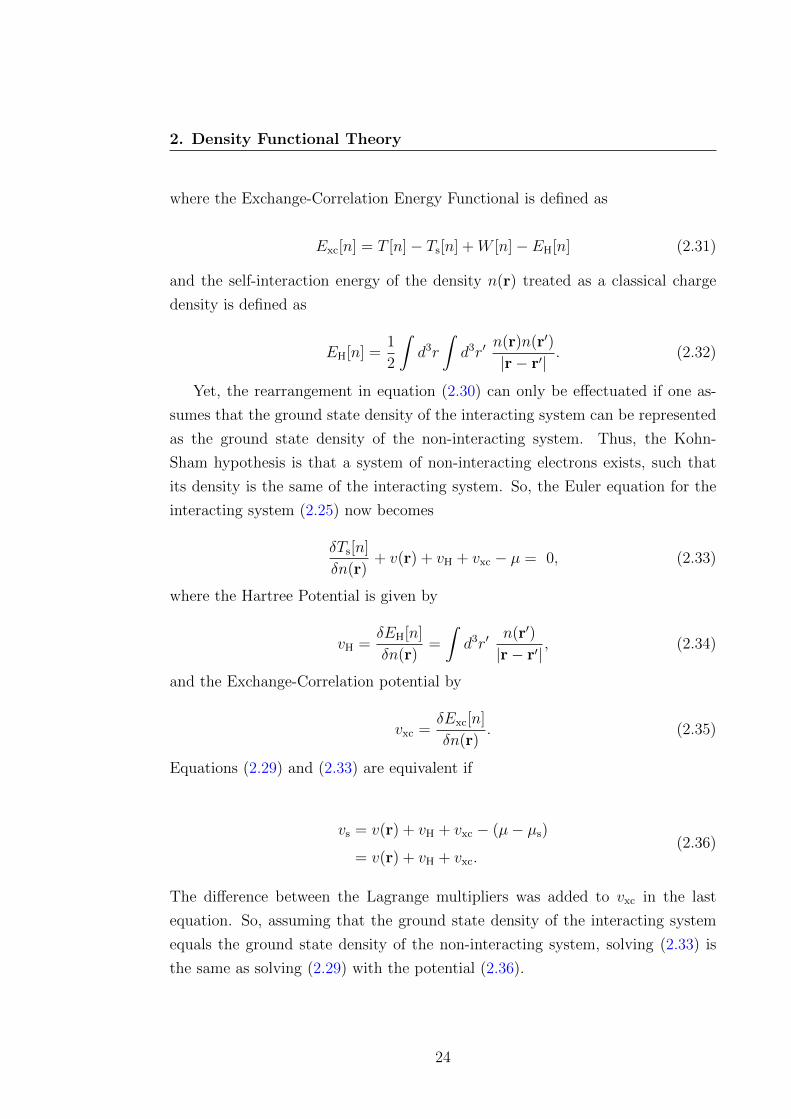
where the Exchange-Correlation Energy Functional is defined as
Exc[n] = T [n]− Ts[n] +W [n]− EH[n] (2.31)
and the self-interaction energy of the density n(r) treated as a classical charge
density is defined as
EH[n] =1
2
∫d3r
∫d3r′
n(r)n(r′)
|r− r′|. (2.32)
Yet, the rearrangement in equation (2.30) can only be effectuated if one as-
sumes that the ground state density of the interacting system can be represented
as the ground state density of the non-interacting system. Thus, the Kohn-
Sham hypothesis is that a system of non-interacting electrons exists, such that
its density is the same of the interacting system. So, the Euler equation for the
interacting system (2.25) now becomes
δTs[n]
δn(r)+ v(r) + vH + vxc − µ = 0, (2.33)
where the Hartree Potential is given by
vH =δEH[n]
δn(r)=
∫d3r′
n(r′)
|r− r′|, (2.34)
and the Exchange-Correlation potential by
vxc =δExc[n]
δn(r). (2.35)
Equations (2.29) and (2.33) are equivalent if
vs = v(r) + vH + vxc − (µ− µs)
= v(r) + vH + vxc.(2.36)
The difference between the Lagrange multipliers was added to vxc in the last
equation. So, assuming that the ground state density of the interacting system
equals the ground state density of the non-interacting system, solving (2.33) is
the same as solving (2.29) with the potential (2.36).
24

2. Density Functional Theory
Therefore, for a given vs, one obtains the density n(r) that satisfies (2.33) by
solving the N one-electron equations (2.26), since solving (2.29) is the same as
solving (2.26). This yields the Kohn-Sham equations.
2.4 Kohn-Sham Equations and Eigenvalues
The Kohn-Sham equations can then be written as
[− ∇
2
2+ vKS[n](r)
]ϕi(r) = εiϕi(r). (2.37)
The Kohn-Sham equations describe non-interacting electrons that move subject
to an effective potential, the Kohn-Sham potential, that has the form
vKS[n](r) = vext(r) + vHartree[n](r) + vxc[n](r). (2.38)
Besides, one should expect no simple physical meaning for the Kohn-Sham wave-
functions ϕi(r) and eigenvalues εi. With the exception of the highest occupied
eigenvalue, which is, approximately, minus the ionization potential I
maxoccupied
εi ' −I (2.39)
there is none. Nevertheless, the density can be obtained from the Kohn-Sham
wave functions as in equation (2.27).
Due to the functional dependence on the density, the Kohn-Sham equations
form a set of non-linear coupled equations. The typical procedure to solve them
is by iterating until self-consistency is achieved [12] (in a Self Consistent Field
Cycle as depicted in figure 2.3). Normally, an initial density is supplied to start
the iterative procedure.
25

2. Density Functional Theory
Figure 2.3: Flow chart depicting the Kohn-Sham SCF cycle.
Would the exact form of the exchange-correlation energy functional be known,
solution of the Kohn-Sham equations should yield the exact ground state density
and energy for the interacting system. Alas, the exact exchange correlation energy
functional is not known and, therefore, has to be approximated.
2.4.1 Spin Density Form
The aforementioned Kohn-Sham equations are only valid in the spin-independent
formalism. Regardless, DFT can be formulated within a spin-dependent formal-
ism which account for external potentials with magnetic terms and spin depen-
dences in the external potential or in the exchange-correlation functional (SDFT
[18, 19]). Here is only presented the special case of a collinear spin polarized
system with no external magnetic field applied and mz will be referred to as the
magnetization density because m = (0, 0,mz)) for a collinear spin system.
Let the ground state electron density and the magnetization density mz have
26

2. Density Functional Theory
the form
n(r) = n↑(r) + n↓(r)
mz(r) = n↑(r)− n↓(r),(2.40)
where
nσ(r) =N∑i
|ϕσi (r|2. (2.41)
For this system, there are two sets of Kohn-Sham equations (one for spin up and
another for spin down)
[− ∇
2
2+ vσext(r) + vHartree[n](r) + vσxc[n,mz](r)
]ϕσi (r) = εσi ϕ
σi (r). (2.42)
Once again, with the Kohn-Sham equations in this form, collinear spin polarized
systems can be described.
2.4.2 Relativistic Density Form
Sometimes relativistic effects are too important to be ignored and a relativistic
extension of DFT has to be applied (RDFT [3, 20, 21]). With the assumption
of collinearity, for the case where there is only an external scalar potential, no
magnetic field and the system is not polarized, the Kohn-Sham equations can be
extended to Dirac-like equations
[icα · ∇+ (β − 1)c2 + vKS(r)
]ϕi(r) = εiϕi(r), (2.43)
where α and β are the usual Dirac matrices, vKS is the usual Kohn-Sham potential,
and the wavefunctions ϕi are four-component spinors. The density is evaluated
as
n(r) =∑i
ϕ†i (r)ϕi(r). (2.44)
27

2. Density Functional Theory
2.5 Exchange and Correlation Functionals
The exchange and correlation energy can be divided in two terms: the ex-
change energy and the correlation energy
Exc[n] = Ex[n] + Ec[n] =
∫d3r n(r)[εx(n(r)) + εc(n(r))], (2.45)
where εxc = εx + εc is the exchange correlation energy per particle of the system.
The exchange energy can be related with the self-interaction correction (a classical
effect which guarantees that an electron cannot interact with itself), and with the
Pauli exclusion Principle, which tends to keep two electrons with parallel spin
apart in space. While the correlation energy have connections to the Coulomb
repulsion, which tends to keep any two electrons apart in space.
This energy functional has to be approximated as its correct form is unknown.
The simplest approximation, and also the first is the local spin density approxi-
mation (LSDA, or only LDA for simplicity). Other example is the quite popular
generalized gradient approximation (GGA).
2.5.1 Local Density Approximation
The LDA for the exchange-correlation energy was proposed in the original
work of Kohn and Sham [16] and can be written as
ELDAxc [n↑, n↓] =
∫d3r n(r)εHEG
xc (n↑(r), n↓(r)), (2.46)
where the exchange-correlation energy density of the system at a given point is
equal to the exchange-correlation energy of the homogeneous electron gas. The
exchange part is known analytically whereas the the correlation part is only known
in the limits of high and low densities. Some points in between were generated
by Monte-Carlo simulations [22]. Due to its relation to the homogeneous electron
gas, it should work well only with fairly homogeneous systems. Surprisingly, it
works well with inhomogeneous systems. It describes very well some physical
properties of atoms, molecules and solids (like equilibrium geometries). But it
also presents large errors (in eigenvalues per example).
28

2. Density Functional Theory
2.5.2 Generalized gradient approximation
An improvement over LDA is the well known GGA. This approximation main-
tains correct physical features of the LDA and introduces a dependence on gra-
dients of the density
EGGAxc [n↑, n↓] =
∫d3r n(r)εGGA
xc (n↑(r), n↓(r),∇n↑(r),∇n↓(r)). (2.47)
To construct the exchange correlation energy functional one has to force the
functional to obey some known physical constraints while avoiding problems with
large gradients. While presenting good results for the energy calculations, most
GGA, like the LDA, fail to reproduce the asymptotic behaviour of the exchange-
correlation potential.
2.5.2.1 PBE
There are many examples of GGA functionals, like the GGA proposed by
Perdew, Burk and Ernzerhof (PBE [23, 24] ). The exchange part is given by
εPBEx = εHEG
x FPBEx
FPBEx = 1 + k − k
1 + (µs2/k),
(2.48)
where k = 0.804 and µ = 0.21951. While the correlation part is chosen as
εGGAxc = εHEG
c +H(rs, ζ, t), (2.49)
where (n↑ − n↓)/n is the spin polarization, rs is the local value of the density
parameter, and t = |∇n|/(2φkTFn) is a dimensionless gradient. Here φ = [(1 +
ζ)2/3 + (1− ζ)2/3]/2 and H is given by
H =e2γφ3
a0
log(1 +
βt2
γ
1 + At2
1 + At2 + A2t4). (2.50)
29

2. Density Functional Theory
The function A represents
A =β
γ
[e−a0ε
HEGc
e2γφ3 − 1
]−1
. (2.51)
30

2. Density Functional Theory
31

Chapter 3
Time Dependent Density
Functional Theory
The only reason for time is so that everything doesn’t happen at once.
Albert Einstein
3.1 A look into TDDFT
Time... TDDFT [25, 26] can be viewed as an exact reformulation of the time-
dependent quantum mechanics, where the many body wave function is replaced in
favor of the density. As DFT revolutionized electronic structure, by introducing
the necessary machinery to obtain all the ground state properties of a system,
TDDFT is proving to be a worthy extension both in name as in achievements.
The methods to obtain the response of a system to an applied field, as propagation
of the Kohn-Sham equations through time, have proven to be a remarkable way
to study the excited states of a system, mainly for the possibilities they provide.
3.2 Runge-Gross Theorem
The time-dependent Schrodinger equation can be written as
i∂
∂tΨ(t) = H(t)Ψ(t) = T + W + V (t)Ψ(t), (3.1)

3. Time Dependent Density Functional Theory
where T and W are taken as in (1.3) and (1.5), and the time dependence of the
Hamiltonian comes from a time dependent potential that may be expressed as
V (t) =N∑i=1
v(r, t). (3.2)
This potential includes the interaction between electrons and nuclei and an ad-
ditional time-dependent term.
In order to formulate a proper Time-Dependent Density Functional Theory,
one has to prove the Runge-Gross theorem [27], the time-dependent extension of
the ordinary Hohenberg-Kohn theorem formulated in 1984.
Theorem 1 For every potential v(r, t) which can be expanded into a Taylor series
with respect to the time coordinate around t = t0, a map G : v(r, t) −→ n(r, t)
is defined by solving the time-dependent Schrodinger equation with a fixed initial
state Ψ(t0) = Ψ0 and calculating the corresponding densities n(r, t). This map
can be inverted up to an additive merely time-dependent function in the potential.
To prove this theorem, one has to show that two densities n(r, t) and n′(r, t) evolv-
ing from the same initial state Ψo through the influence of the potentials v(r, t)
and v′(r, t), respectively, are always different by more than a time-dependent
function
v(r, t) 6= v′(r, t) + c(t). (3.3)
If this is true, the map G, defined as surjective in the theorem, is also injective
G : v(r, t) ←→ n(r, t) (3.4)
and can then be inverted. This one to one correspondence means that the time-
dependent density determines the potential up to a purely time-dependent func-
tion and, therefore, the wavefunction is determined up to a purely time-dependent
phase and can be expressed as a functional of the density and the initial state:
Ψ(t) = eiα(t)Ψ[n,Ψ0](t). (3.5)
33

3. Time Dependent Density Functional Theory
Consequently, the expectation value of any hermitian operator can also be re-
vealed to be a functional of the density and the initial state
Q[n,Ψ0](t) = 〈Ψ[n,Ψ0](t)| O(t) |Ψ[n,Ψ0](t)〉 . (3.6)
The proof of the theorem can be divided in two steps. The first step consists
in proving that different potentials, v(r, t) and v′(r, t), acting on the same initial
state, originate different current densities j(r, t) and j′(r, t). The current density
can be obtained from
j(r, t) = 〈Ψ(t)| j |Ψ(t)〉 , (3.7)
using the paramagnetic current density operator
j(r) =1
2i
N∑i=1
[∇iδ(r− ri) + δ(r− ri)∇i
]. (3.8)
As the initial state is the same for both primed and unprimed systems
Ψ(r, t = 0) = Ψ′(r, t = 0) = Ψ0,
n(r, t = 0) = n′(r, t = 0) = n0(r),
j(r, t = 0) = j′(r, t = 0) = j0(r),
(3.9)
the application of the equation of motion for the expectation value of the current
density,
∂
∂t〈Ψ(t)| j(r) |Ψ(t)〉 = 〈Ψ(t)| ∂ j
∂t− i[j(r), H(t)] |Ψ(t)〉 , (3.10)
yields
∂
∂tj(r, t) =
∂
∂t〈Ψ(t)| j(r) |Ψ(t)〉 = −i 〈Ψ(t)| [j(r), H(t)] |Ψ(t)〉
∂
∂tj′(r, t) =
∂
∂t〈Ψ′(t)| j(r) |Ψ′(t)〉 = −i 〈Ψ′(t)| [j(r), H ′(t)] |Ψ′(t)〉 .
(3.11)
Taking the difference of the last equations and evaluating it at the initial time
34
3. Time Dependent Density Functional Theory
results in
∂
∂t
[j(r, t)− j′(r, t)
]t=0
= −i 〈Ψ0| [j(r), H(0)− H ′(0)] |Ψ0〉
= −i 〈Ψ0| [j(r), V (0)− V ′(0)] |Ψ0〉
= −n0(r)∇[v(r, 0)− v′(r, 0)
].
(3.12)
Now if[v(r, 0)−v′(r, 0)
]is different than a constant, the right hand side of (3.12)
cannot vanish identically and the current densities will become different infinitesi-
mally later than t = 0. But this may not be true. Nevertheless, for potentials that
can be expanded as a Taylor series with respect to the time coordinate around t
= 0
v(r, t) =∞∑k=0
tk
k!
[ ∂k∂tk
v(r, t)]t=0
(3.13)
the condition (3.3) is equivalent to statement that there is a integer k ≥ 0 such
that
wk(r) =∂k
∂tk
[v(r, t)− v′(r, t)
]t=0
6= 0. (3.14)
So, application of the equation of motion (k + 1) times produces
∂k+1
∂tk+1
[j(r, t)− j′(r, t)
]t=0
= −n0(r)∇wk(r) 6= 0. (3.15)
Once more, infinitesimally later than the initial time,
j(r, t) 6= j′(r, t). (3.16)
Therefore, this first step of the proof of the Runge-Gross theorem proves a one
to one correspondence between potentials and current densities.
Similarly, the second step of the proof consists in proving that two different
current densities imply two different densities. For that one uses the continuity
equation,∂
∂tn(r, t) = −∇ · j(r, t), (3.17)
to calculate the (k+ 2) time-derivative of the both densities (n(r, t) and n′(r, t)).
35

3. Time Dependent Density Functional Theory
Taking the difference of the two at the initial time and using (3.14) results in
∂k+2
∂tk+2
[n(r, t)− n′(r, t)
]t=0
= ∇ ·[n0(r)∇wk(r)
]. (3.18)
Hence, if ∇ ·[n0(r)∇wk(r)
]6= 0, then the densities are different, which proves a
one to one correspondence between the densities and the currents. To prove this,
consider the integral∫d3r wk(r)∇ ·
[n0(r)∇wk(r)
]= −
∫d3r n0
[∇wk(r)
]2+
+
∮S
dS ·[n0(r)wk(r)∇wk(r)
],
(3.19)
where Green’s theorem has been used. For potentials arising from normalizable
external charge densities, the surface integral on the right vanishes. Besides, the
remaining integrand on the right (n0
[∇wk(r)
]2) is strictly positive (or zero if the
density is also zero, which is not intended). As a consequence, the integrand on
the left has to be different than zero. Then ∇ ·[n0(r)∇wk(r)
]cannot be zero
everywhere and the proof of the Runge-Gross theorem is complete.
3.3 Time-Dependent Kohn-Sham Equations
Having established the Runge-Gross theorem, it is possible to construct a
time-dependent Kohn-Sham scheme. First, one defines an auxiliary system of
non-interacting electrons subjected to an external local potential vKS. The Runge-
Gross theorem states that this potential is unique and is chosen in a way that the
density of the Kohn-Sham electrons is the same as the density of the original in-
teracting system. Moreover, the Kohn-Sham electrons satisfy the time-dependent
Scrodinger equation
i∂
∂tϕi(r, t) =
[− ∇
2
2+ vKS[n,Ψ0,Φ0](r, t)
]ϕi(r, t), (3.20)
36

3. Time Dependent Density Functional Theory
whose orbitals provide the same density as the density of the interacting system:
n(r, t) = 〈Φ(t)|∑i
δ(r− ri) |Φ(t)〉 =N∑i
|ϕi(r, t)|2. (3.21)
The time-dependent Kohn-Sham potential vKS can be decomposed into:
vKS[n,Ψ0,Φ0](r, t) = vext[n,Ψ0](r, t)+vHartree[n](r, t)+vxc[n,Ψ0,Φ0](r, t). (3.22)
This means that the difference between the external potential, that generates the
density n(r, t) in an interacting system with initial state Ψ0, and the one-body
potential, that generates the same density in a non-interacting system with initial
state Φ0, is the xc potential added to the classical Hartree potential
vHartree[n](r, t) =
∫d3r′
n(r′, t)
|r− r′|. (3.23)
The external potential in vKS can be conveniently defined as
vext[n,Ψ0](r, t) = vext0[n,Ψ0](r) + θ(t− t0)vper[n](r, t), (3.24)
that is, at t < t0 the system is at the ground state under the effect of a static
potential whilst at t ≥ t0 a time-dependent potential is applied to the system.
In this construction, the xc potential includes all non-trivial many body effects
and has an extremely complex functional dependence on the density. Quantum
mechanics shows that minimization of the total energy yields the ground state of
a system. However, as the energy is not a conserved quantity in a time-dependent
system subject to a time-dependent external potential, there can be no variational
principle on the basis of the total energy. Still, there is an analogous quantity to
the ground state energy, the quantum mechanical action
A[Ψ] =
∫ t1
t0
dt 〈Ψ(t)| i ∂∂t− H(t) |Ψ(t)〉 , (3.25)
where Ψ(t) is a N-body function. Unfortunately, using this action to define the
xc potential, as vxc(r, t) = δAδn(r,t)
, results in causality and boundary conditions
problems. These problems were solved by van Leeuwen [28] by using the Keldysh
37

3. Time Dependent Density Functional Theory
formalism and by introducing a new action functional A for which the xc potential
could be written as a variation of this new action without problems. Yet this new
functional dependence on the density is still immensely complex.
3.4 Adiabatic Approximation for Functionals
As the DFT exchange-correlation energy functional, the TDDFT xc potential
is also unknown. This functional depends on the time-dependent density, which
means that, rigorously, vxc[n](r, t) depends on the entire history of the density.
There are few xc functionals that satisfy this computationally demanding condi-
tion. On the contrary, there is a plethora of ground state xc functionals available
for DFT, as the result of more than 46 years of active research. The adiabatic
approximation neglects the time-dependence condition while taking advantage of
the existing ground state xc functionals.
The adiabatic time dependent xc potential takes the form
vxc[n](r, t) = vxc[n](r)|n=n(r,t), (3.26)
for spin-independent TDDFT, and
vσxc[n↑, n↓](r, t) = vσxc[n
↑, n↓](r)|nσ=nσ(r,t), (3.27)
for the spin-dependent version of TDDFT [29]. This quite dramatic approxima-
tion is expected to work only in cases where the temporal dependence is small,
that is, when the time-dependent system is locally close to equilibrium.
Regardless of its problems in describing the situations when the electrons get
away from the nuclei, the adiabatic local density approximation (ALDA), which is
the simplest approximation for the TDDFT xc functional, yields remarkably good
excitation energies for many systems. The AGGA (adiabatic generalized gradient
approximation) xc functional is expected to behave in a similar way, having the
same problems which arise from an incorrect asymptotic behaviour (the potential
do not decay as−1/r) while reasonably describing the true response of the system.
Actually, both ALDA and AGGA provide similar excitation energies, as the KS
orbital energy differences are reasonably good approximations to those energies
38

3. Time Dependent Density Functional Theory
and the xc kernel only has to add a small correction on top of that estimate. In
fact, simple approximations provides good results while similar approximations
provide almost identical results.
3.5 Response Functions
In spectroscopic experiments, a sample is subjected to an external field F (r, t).
Then, the sample, which is a fully interacting many-body system, responds to the
field. This response can be measured by the change of some physical observable
P:
∆P = ∆PF [F ]. (3.28)
Clearly, as this functional has to reproduce the response for a field of any
strength and shape, the dependence of the functional ∆PF on F is very complex.
Nevertheless, for a weak field, the response can be expanded as a power series
with respect to the field strength.
The first order response of an observable consists on a convolution of the linear
response function χ(1)P←F with the variation of the field δF (1), expanded to the
first order in the field strength.
δP(1)(r, t) =
∫dt′∫d3r′ χ
(1)P←F (r, r′, t, t′)δF (1)(r′, t′), (3.29)
where
χ(1)P←F (r, r′, t, t′) =
[δP(1)(r, t)
δF (1)(r′, t′)
]δF (1)(r′,0)
. (3.30)
The linear response can also be cast in terms of the frequency ω in frequency
space
δP(1)(r, ω) =
∫d3r′ χ
(1)P←F (r, r′, ω)δF (1)(r′, ω). (3.31)
On the other hand, second-order response can be written as
39

3. Time Dependent Density Functional Theory
δP(2)(r, t) =1
2
∫dt′∫dt′′∫d3r′
∫d3r′′ ×
χ(2)P←F (r, r′, r′′, t, t′, t′′)δF (1)(r′, t′)δF (1)(r′′, t′′)
+
∫dt′∫d3r′ χ
(1)P←F (r, r′, t− t′)δF (2)(r′, t′).
(3.32)
Higher-order responses have a similar straightforward construction withal.
3.5.1 Linear Response and Photo-absorption Spectra
One of the most important response functions is the linear density response
function
δn(r, ω) =
∫d3r′ χn←vper(r, r
′, ω)δvper(r′, ω), (3.33)
which gives the linear response of the density to an external scalar perturbative
potential δvper(r′, ω). If the density response function χn←vper(r, r
′, ω) can be cal-
culated, it can be used to obtain the first-order response of all properties derivable
from the density with respect to any scalar field. An example is the polarizability
α. Consider a finite system of electrons and nuclei which are subjected to an elec-
trical field E. The response of the system to this electrical field is characterized
by a variation of the time-dependent induced electrical dipole moment µ, which
for finite systems can be expressed as a Taylor expansion [30]
µi = µi0 +∑j
αij(ω)Eωj +
∑j,k
1
2!βijk(ω)Eω1
j Eω2k +
+∑j,k,l
1
3!γijkl(ω)Eω1
j Eω2k E
ω3l + ...,
(3.34)
where the indices refer to spatial coordinates, α is the linear polarizability, β and
γ are hyperpolarizabilities, and in each term ω =∑
m ωm (i.e. in the second term
ω = ω1 + ω2). For a weak field
40
3. Time Dependent Density Functional Theory
δµ(ω) = −α(ω)E(ω), (3.35)
where µ(ω) is the induced dipole moment δµ(t) = µ(t)− µ(0) in the frequency
domain. However, the dipole moment can also be calculated as
µ(t) = −N∑i=1
〈ϕi(t)| r |ϕi(t)〉 = −∫d3r rn(r, t). (3.36)
Therefore, the polarizability is given by
αij(ω) =1
Ej(ω)
∫d3r xi δn(r, ω)
=1
Ej(ω)
∫d3r xi
∫d3r′ χn←vper(r, r
′, ω)δvper(r′, ω),
(3.37)
where xi are the components of r. Now, for a dipole electric field along the xj
direction one has δvper(r, t) = −xjEj(t)δ(t). So, replacing the Fourier transform
of this potential in the last equation yields
αij(ω) = −∫d3r
∫d3r′ xi χn←vper(r, r
′, ω)x′j. (3.38)
Moroever, the polarizability can be used to calculate the photo absorption cross-
section
σij(ω) =4πω
c=αij(ω)
. (3.39)
from which one can then obtain the average orientational absorption coefficient
A:
A =1
3Tr[σ(ω)
]=
4πω
c=1
3Tr[α(ω)
]. (3.40)
The photo absorption spectrum can then be obtained by plotting the average
absorption coefficient as a function of the energy.
The polarizabilities α, β and γ shown in (3.34) allude to the electrical spin-
independent response of a system to an applied electrical field. Therefore they
are known as density-density response functions. Nevertheless, if a perturbation
and/or an observable are spin-dependent, one can define more general response
41
3. Time Dependent Density Functional Theory
functions known as susceptibilities [3]. These susceptibilities can refer to density-
density, spin-density, density-spin and spin-spin response functions. When the
perturbation potential acts differently on collinear spin-up and spin-down elec-
trons, the linear response density becomes:
δnσ(r, ω) =∑σ′
∫d3r′ χσσ
′
n←vper(r, r′, ω)δvσ
′
per(r′, ω). (3.41)
This equation shows how to calculate the change in the density (δn) from a
change in the external potential δvext. Based on the spin-up and spin-down
electron density one can define the variations of the total electron density and of
the magnetization density (once again, refers to mz) as
δn(r, ω) = δn↑(r, ω) + δn↓(r, ω) (3.42)
δm(r, ω) = δn↑(r, ω)− δn↓(r, ω). (3.43)
Combination of the last equations with equation (3.41), taken in the form δnσ(r, ω) =∑σ′ F [χσσ
′, δvσ
′] for simplicity, yields:
δn(r, ω) = F [χ↑↑, δv↑] + F [χ↑↓, δv↓] + F [χ↓↑, δv↑] + F [χ↓↓, δv↓]
δm(r, ω) = F [χ↑↑, δv↑] + F [χ↑↓, δv↓]− F [χ↓↑, δv↑]− F [χ↓↓, δv↓].(3.44)
Let the perturbation potentials in the previous equation have the form
δvσ [n]per (r, ω) = −xjEj(ω), (3.45)
for a spin-independent perturbation (indicated by [n]) and,
δvσ[m]per (r, ω) = −xjEj(ω)σz, (3.46)
with σz = 1,−1 if σz = ↑, ↓ for a spin-dependent perturbation (indicated by [m]).
42

3. Time Dependent Density Functional Theory
Inserting these potentials into (3.44) results in
δn[n](r, ω) = −(F [χ↑↑, xjEj] + F [χ↑↓, xjEj] + F [χ↓↑, xjEj] + F [χ↓↓, xjEj]
)δm[n](r, ω) = −
(F [χ↑↑, xjEj] + F [χ↑↓, xjEj]− F [χ↓↑, xjEj]− F [χ↓↓, xjEj]
)δn[m](r, ω) = −
(F [χ↑↑, xjEj]− F [χ↑↓, xjEj] + F [χ↓↑, xjEj]− F [χ↓↓, xjEj]
)δm[m](r, ω) = −
(F [χ↑↑, xjEj]− F [χ↑↓, xjEj]− F [χ↓↑, xjEj] + F [χ↓↓, xjEj]
).
(3.47)
Using equations (3.35) and (3.36) for the dipole moment and similar equations for
the spin-dipole moment (obtained by replacing the density by the magnetization
density, the dipole moment by the spin-dipole moment and considering α as a
first order susceptibility), one finds
α[nn]ij = α↑↑ij + α↑↓ij + α↓↑ij + α↓↓ij
α[mn]ij = α↑↑ij + α↑↓ij − α
↓↑ij − α
↓↓ij
α[nm]ij = α↑↑ij − α
↑↓ij + α↓↑ij − α
↓↓ij
α[mm]ij = α↑↑ij − α
↑↓ij − α
↓↑ij + α↓↓ij ,
(3.48)
where
ασσ′
ij (ω) = −∫d3r
∫d3r′ xi χ
σσ′(r, r′, ω)x′j. (3.49)
The density-density first order susceptibility, α[nn]ij , is the same as the polarizabil-
ity of equation (3.38).
3.5.2 Kohn-Sham Linear Response
The linear response function χ in equation (3.41) is very hard to calculate.
However, TDDFT provides a way to obtain it via the non-interacting Kohn-Sham
system [31]. Variation of the Kohn-Sham potential (3.22) yields
δvσKS(r, ω) = δvσext(r, ω) +
∫d3r
δn(r′, ω)
|(r− (r′|+∑σ′
∫d3r′ fσσ
′
xc (r, r′, ω)δn(r′, ω),
(3.50)
43

3. Time Dependent Density Functional Theory
with δn as in (3.42) and where fσσ′
xc (r, r′, ω) is the Fourier transform of the xc
kernel
fσσ′
xc (r, r′, t− t′) =δvσxc[n↑, n↓](r
′, t′)
δnσ′(r′, t′). (3.51)
Besides, in the Kohn-Sham system, the variation of the density can be written as
δnσ(r, ω) =∑σ′
∫d3r′ χσσ
′
KS (r, r′, ω)δvσ′
KS(r′, ω). (3.52)
The response function in the last equation, the density response function of
the non-interacting electrons, may also be expressed in terms of the unperturbed
stationary Kohn-Sham orbitals
χσσ′
KS (r, r′, ω) = δσσ′∞∑jk
(fkσ − fjσ)ϕjσ(r)ϕ∗jσ(r′)ϕkσ(r′)ϕ∗kσ(r)
ω − (εjσ − εkσ) + iη. (3.53)
Here η is a positive infinitesimal and, as usual, ϕjσ and εkσ are the ground state
Kohn-Sham orbitals and eigenvalues and fjσ indicates the occupation number.
Combining equations (3.50) and (3.52) results in
δnσ(r, ω) =∑τ
∫d3r′χσσ
′
KS (r, r′, ω)
[δvτext(r
′, ω) +
∫d3x
δn(x, ω)
|r′ − x|+
+∑τ ′
∫d3xf ττ
′
xc (r, r′, ω)δnτ′(ω)
].
(3.54)
Finally, inserting (3.41) and using the fact that vext is an arbitrary function,
makes it possible to reveal the response function as a Dyson-like equation
χσσ′(r, r′, ω) = χσσ
′
KS (r, r′, ω)+
+∑ττ ′
∫d3x
∫d3x′χστ (r, r′, ω)
[1
|x− x′|+ f ττ
′
xc (r, r′, ω)
]χτ′σ′
KS (r, r′, ω).
(3.55)
If the exact functional fxc[n↑, n↓] were known, a self-consistent solution of this
44

3. Time Dependent Density Functional Theory
last equation would yield the exact response function of the interacting system.
Of course, there are several approximations to the xc kernel yet, a full solution
of (3.55) is still quite difficult numerically. Fortunately, there are several ways to
circumvent this problem.
3.5.3 Time-Propagation Method
There are at least three ways to calculate response functions from TDDFT:
the Sternheimer method, the Casida Method, and the time-propagation method.
In the Sternheimer method [32], which is a perturbative approach, solves for a
specific order of the response for a specific field in frequency space. Higher-order
responses can be calculated from the lower ones. While in the Casida Method
[33], instead of discovering the response, one calculates the poles and residues
of the first-order response function, which corresponds to finding the resonant
transitions of a system. Finally, the time-propagation method [34] consists in
explicitly propagating the system in time after the application of a perturbing
potential to excite the ground-state. Afterwards the difference between the final
and the initial dipole moment provides a response function.
Only the later method will be discussed here given its importance for this
thesis (all response calculations were carried out using this method). First, one
has to understand how a wavefunction is propagated. The Kohn-Sham equations
and all other Schrodinger like equations may be rewritten in terms of its linear
propagator U(t, t0) as
i∂
∂tU(t, t0) = HKS(t)U(t, t0), (3.56)
which has a solution in terms of the initial state ϕ(r, t0)
ϕ(r, t) = U(t, t0)ϕ(r, t0). (3.57)
The last differential equation can be integrated
U(t′, t) = 1− i
∫ t′
t
dτ HKS(τ)U(τ, t0). (3.58)
45

3. Time Dependent Density Functional Theory
The evolution operator U(t′, t) can be seen as a Dyson operator, therefore it can
be rewritten as a Dyson’s series
U(t′, t) = T e−i∫ t′t dτ HKS(τ). (3.59)
Three properties of U(t′, t) can be derived from its definition:
• For a Hermitian Hamiltonian, U(t′, t) is unitary.
U †(t+ ∆t, t) = U−1(t+ ∆t, t) (3.60)
• U(t′, t) has time reversal symmetry.
U(t+ ∆t, t) = U−1(t, t+ ∆t) (3.61)
•U(t1, t2) = U(t1, t3)U(t3, t2).
Therefore ϕ(t) can be propagated in small time steps
U(t+ ∆t, t) = T e−i∫ t+∆tt dτ HKS(τ). (3.62)
Application of (3.62) is not trivial and to proceed further, one has to find
an approximation for the full time-evolution operator, which are based on the
approximation of the exponential of an operator. Luckily, there are several algo-
rithms to approximate eˆO(t), like polynomial expansions, Krylov subspace projec-
tion techniques and splitting schemes, and therefore, a handful of approximations
for the time-dependent propagator, based on Magnus Expansions, the Exponen-
tial Midpoint Rule and splitting techniques (for more information one should
check [25]).
An example of an approximation for U , the enforced time-reversal symmetry
method is presented: as in a time-reversible method, propagating backwards ∆t2
starting from ϕ(t+∆t) or propagating forwards ∆t2
starting from ϕ(t) should lead
to the same result
e+i ∆t2H(t+∆t)ϕ(t+ ∆t) = e−i ∆t
2H(t)ϕ(t). (3.63)
46

3. Time Dependent Density Functional Theory
Rearranging the terms provides the approximation for the propagator
UETRS(t+ ∆t, t) = e−i ∆t2H(t+∆t)e−i ∆t
2H(t). (3.64)
With this in mind, it is straightforward to understand the time-propagation
method procedure. Let ϕi(r, 0), the solutions of the ground state Kohm-Sham
equations, be the initial state for the system under study, and let vper(t) =
−xjEjδ(t) be the form of the weak electric dipole spin-independent perturba-
tion that excites the electrons of the initial state. Let also the Kohn- Sham
Hamiltonian be written like HKS(t) = H0KS(t) + vper(t).
First, one needs to find ϕi(r, 0). The ground state is then perturbed at t = 0.
The wavefunctions at t = 0+ can be calculated using
ϕi(r, 0+) = T e−i
∫ 0+
0 dτ[H0
KS(τ)+vper(τ)]ϕi(r, 0)
= T e−i∫ 0+
0 dτ[H0
KS(τ)−xjEjδ(τ)]ϕi(r, 0)
= eixjEjϕi(r, 0).
(3.65)
This phase-factor shifts the momentum of the electrons, giving them a coherent
velocity field that causes the appearance of a polarization as the system evolves
in time.
Finally, the system is propagated up to some finite time using recursively
(3.62). Then the time-dependent dipole moment (3.36) can be used to extract
the dynamic polarizability tensor
αij =1
Kj
∫ ∞0
dt[µi(t)− µi(0)
]e−iωte−ηt +O(Kj), (3.66)
where e−iωt comes from the Fourier transform and e−ηt is a damping function
attached because infinite time-propagation is not possible in practice. The photo-
absorption Spectrum is obtained by calculating the average absorption coefficient
as in (3.40) and plotting it as a function of the energy.
47
Part III
Numerical Aspects


Chapter 4
Pseudopotential Approximation
It always bothers me that according to the laws as we understand them today,
it takes a computing machine an infinite number of logical operations to figure
out what goes on in no matter how tiny a region of space and no matter how
tiny a region of time ...
Richard Feynman
4.1 A look into Pseudopotentials
Computing... The nuclear attractive potential binds electrons to nuclei,
those that are more bound are normally defined as inner core electrons while
those that move more freely, and thus have a greater probability of binding with
other atoms, are designated as valence electrons. In fact, binding properties are
almost completely due to the valence electrons. Besides, near the nucleus, the
valence electrons’ wave functions oscillate rapidly due to the orthogonalization
between wavefunctions. Actually, oscillations of the wave function can be trans-
lated into more kinetic energy to the electrons, which cancels the nucleus strong
attractive potential and explains why the valence electrons move more freely and
are lesser bound to the nuclei. Nevertheless, these oscillations hinder the elec-
tronic structure calculations, as computing becomes more demanding.
This motivates the pseudopotential approximation in which the strong Coulomb
potential of the nucleus and the effects of the tightly bound core electrons are re-
4. Pseudopotential Approximation
placed by an effective (usually weaker) ionic potential acting on valence electrons,
the pseudopotential.
Pseudopotentials have been presented in several creative ways in their long
lasting history [12]. Starting with Fermi’s effective interaction in scattering ex-
periments, they evolved to empirical pseudo-potentials based on the Phillips and
Kleinman cancelation idea, like the Ashcroft potential. With Topp and Hopfield
suggestion, that the pseudopotentials should be adjusted in a way they accu-
rately describe the valence charge density, the ab-initio pseudopotentials were
born. Two examples of this family are the Norm-Conserving pseudopotentials of
Hamann, Schluter, and Chiang, described in this chapter, and the Vanderbilt’s
Ultra-Soft pseudopotentials, where the charge deficit resulting from the relaxation
of the norm-conservation constraint is cancelled by a localized atom-centered aug-
mentation charge.
The study of pseudopotentials has attracted so many people due to their
importance to DFT. Pseudopotentials permit a much faster resolution of the
Kohn-Sham equations while providing accurate results. Therefore, they are in
part responsible for the wild sucess and quick proliferation of DFT.
4.2 Phillips and Kleinman Formal Construction
The Phillips and Kleinman Formal Construction of a Pseudopotential can be
traced back to the orthogonalized plane wave method (OPW) [35], in which the
valence wavefunctions |ϕv〉 were expanded in a plane wave basis orthogonal to the
inner core states |ϕc〉. Let both groups of wavefunctions be the exact solutions
of the Schrodinger equation with Hamiltonian H. The valence wavefunctions can
then be written as a sum of a smooth function (the pseudo wavefunction |ϕv〉)with an oscillating function related to the inner core wavefunctions:
|ϕv〉 = |ϕv〉+∑c
αcv |ϕc〉 . (4.1)
Application of 〈ϕc| on the left side results in αcv = −〈ϕc|ϕv〉. Therefore, the
Schrodinger equation for the smooth orbital can be written as
51

4. Pseudopotential Approximation
H |ϕv〉 = Ev |ϕv〉+∑c
(Ec − Ev) |ϕc〉 〈ϕc| |ϕv〉 . (4.2)
Thus, the pseudo wavefunctions satisfy a Schrodinger like equation, whose pseudo
Hamiltonian HPK has an additional energy-dependent contribution
HPK(E) = H −∑c
(Ec − E) |ϕc〉 〈ϕc| (4.3)
or, after explicitly writing both Hamiltonians,
vPK(E) = v −∑c
(Ec − E) |ϕc〉 〈ϕc| , (4.4)
where vPK is the Phillips and Kleinman pseudopotential and v is the true poten-
tial. Outside the core region, vPK becomes equal to v due to the decay of the
inner core states whereas, in the vicinity of the core, the pseudo potential be-
comes much weaker because of the additional repulsive contribution (the second
term in (4.4)).
4.3 Norm-conserving Ab-Initio Pseudopotentials
When chasing for the perfect pseudopotential, there are two goals to have in
mind: the pseudopotential should be as soft as possible and as transferable as
possible. A soft pseudopotential means that pseudo wavefunctions can be ex-
panded in less basis functions (like plane-waves), while transferability means that
the pseudopotential can correctly describe different configurations, like crystals
and molecules.
The quest for the perfect pseudopotential has lead to the norm-conserving
pseudopotentials. In spite of existing better pseudopotentials by now, these norm-
conserving pseudopotentials are widely used, partially for their simplicity and
mainly for their capability at providing accurate results with reasonable speed.
Norm-conserving pseudopotentials are obtained through the following proce-
dure [12] [36]:
1. Taking into account all electrons, the free atom radial Kohn-Sham equations
52

4. Pseudopotential Approximation
are solved, for a given configuration, in order to obtain the all electron wave
functions.
As a Schrodinger like equation, the Kohn-Sham equation has a similar reso-
lution. A spherical averaging of the density leads to a spherically symmetric
Kohn-Sham potential. Then, a separation of variables in the wavefunction
leads to the spherical harmonics and to the one-dimensional second-order
equation
[− 1
2
d2
dr2− 1
r
d
dr+l(l + 1)
2r2+ vAE
KS [nAE](r)]RAEnl (r) = εnlR
AEnl (r), (4.5)
where
vAEKS [nAE](r) = −Z
r+ vHartree[n
AE](r) + vxc[nAE](r). (4.6)
There are many methods to solve this equation, like the Shooting method.
2. Imposing the norm-conservation and other specific conditions, the pseudo
wavefunctions are determined using a proper scheme. Denoting the core
radius as rcl, where l stands for the dependency of the core radius with the
angular moment quantum number, these conditions can be written as
εPPl = εAE
nl
Ql =
∫ rcl
0
dr|RPPl (r)|2r2 =
∫ rcl
0
dr|RAEnl (r)|2r2, if
RPPl (r) = RAE
nl (r) if r > rcl.
(4.7)
That is, the pseudo eigenvalues should match the true valence eigenvalues,
the integrated charge inside the core radius for the wavefunction and for the
pseudo wavefunction agrees and, the pseudo and the all electron wave func-
tion are equal beyond the core radius. Besides, the pseudo wavefunctions
should not have nodal surfaces.
Two examples of schemes for the generation of the pseudopotential are
53
4. Pseudopotential Approximation
the Hamann Potential [37] and the Troulier-Martins Potential [38]. The
latter scheme will be presented, as it was the one used to generate norm-
conserving pseudopotentials in this thesis. In the Troulier-Martins scheme,
the wave functions are defined as
RPPl (r) =
RAEnl (r), if r > rcl
rlep(r), if r ≤ rcl,(4.8)
with
p(r) =∑i
c2ir2i with i ∈ [0, 6]. (4.9)
These coefficients are adjusted imposing the continuity of the pseudo wave-
functions and their derivatives until the fourth order at r = rcl, norm con-
servation and that the screened pseudo potential has zero curvature at the
origin.
Additionally, the Troullier-Martins Scheme can be extended in order to
include semi core states into the valence space. This extension is known as
multi-reference pseudopotentials and the difference for the normal Troullier-
Martins scheme is three additional terms in (4.9). The new polynomial have
to be adjusted using the same conditions as the ones used for the normal
scheme applied to the semi-core pseudo wavefunctions and imposing the
conditions (4.7) to the valence pseudo wavefunction.
3. Inversion of the radial Kohn-Sham equation for the pseudo wavefunction
and the valence electron density results in the screened pseudopotential.
vPP,screenedl (r) = εPP
l −l(l + 1)
2r2+
1
2rRPPl (r)
d2
dr2[rRPP
l (r)] (4.10)
4. Finally, subtraction of the Hartree and exchange-correlation potentials yield
the unscreened pseudopotential.
vPP(r) = vPP,screened(r)− vHartree[nPP]− vxc[nPP](r) (4.11)
54

4. Pseudopotential Approximation
55

Chapter 5
The Projector Augmented Waves
Method
Resistance is useless.
Doctor Who
5.1 A look into the PAW Method
Resistance... First introduced and implemented by Blochl [39], the Projector
Augmented Waves Method is an alternative to the pseudopotential approach.
Since then it has been implemented in several codes, like ABINIT [40] and VASP
[41, 42]. Although there was some resistance to use this method in the work
presented in this thesis, this method proved to be faster and more efficient than
methods based on norm-conserving pseudopotentials.
The PAW consists in dividing space in two regions: atom-centered augmen-
tation spheres and an interstitial region. Throughout space, the wave function
can be described by a pseudo wavefunction as in the pseudopotential approach.
Nonetheless, within the augmentation region that description is a poor one. So,
the idea behind the PAW method is to have all electron partial-waves functions
inside those regions. Partial or atomic wave functions are only defined inside the
augmentation region.

5. The Projector Augmented Waves Method
Figure 5.1: The All-electron PAW wavefunction as a sum of the pseudowavefunction with the atomic partial wavefunction subtracted by the partial
pseudo wavefunction.
The easiest way to do so, is to remove the pseudo wave function by subtract-
ing a partial or atomic pseudo wavefunction while summing all electron atomic
functions inside the augmentation region
|ϕ〉 = |ϕ〉+∑i
ci(|ξi〉 − |ξi〉). (5.1)
This expression can be easily derived by expanding both the all electron and the
pseudo wavefunctions in their respective partial-waves inside the augmentation
sphere.
Obviously, for the wavefunction and its gradient to be continuous, an all
electron partial-wave and its pseudo partial-wave must have the same logarithmic
derivative at the boundary of the augmentation region.
Therefore, the PAW method precision and efficiency can already be explained:
as the space is divided into two regions, so is the discretization of the functions.
The smooth pseudo wavefunctions are evaluated on regular uniform grids and in
contrast, the partial-waves are evaluated for each sphere individually on a radial
grid. Consequently, one can have normal discretization in the interstitial region
and a better one for the all electron functions inside each augmentation sphere.
5.2 Formalism
5.2.1 Transformation operator
In order to determine the transformation that changes the pseudo wavefunc-
tion to the wavefunction, one has to calculate the ci coefficients of (5.1).
57

5. The Projector Augmented Waves Method
In the PAW method, this is done by defining the projectors pi, which are localized
inside augmentation spheres. These projectors are required to fulfill the condition
that the one center expansion of a pseudo wavefunction is identical to itself,∑i |ξi〉 〈pi|ϕi〉 = |ϕi〉. Therefore, in the limit ξi forms a complete sum:∑
i
|ξi〉 〈pi| = 1. (5.2)
This implies that the projectors obey the orthonormality condition:
〈pi|ξj〉 = δij. (5.3)
Finally, applying these relations and some algebra tricks to (5.1) ,
|ϕ〉 = (1−∑i
1i) |ϕ〉+∑i
ci(|ξi〉 − |ξi〉)+
+∑i
|ξi〉 〈pi|ϕi〉(5.4)
results in
ci = 〈pi|ϕi〉 . (5.5)
Then, the transformation operator takes the form
T = 1 +∑i
(|ξi〉 − |ξi〉) 〈pi| . (5.6)
It can be used to write
|ϕj〉 = T |ϕj〉 (5.7)
5.2.2 Operators
The PAW pseudo operators (O) can be obtained from the all-electron opera-
tors (O) using (5.7):
〈ϕi| O |ϕj〉 = 〈ϕi| T†OT |ϕj〉 = 〈ϕi| O |ϕj〉 . (5.8)
58

5. The Projector Augmented Waves Method
The form of the pseudo operator O = T†OT had to be evaluated both inside
and outside the augmentation region ΩR. Within the augmentation region, some
terms will cancel as a consequence of (5.2) and
O =∑ij
|pi〉 〈ξi| O |ξj〉 〈pj| . (5.9)
While outside the augmentation region the partial waves are equal |ξi〉 = |ξi〉, so
O = O. (5.10)
Therefore, the pseudo operator can be written independently of the region of
space where it is being evaluated as
O = T†OT = O +∑ij
|pi〉 (〈ξi| O |ξj〉 − 〈ξi| O |ξj〉) 〈pj| . (5.11)
As an example, one can use the charge density operator and the later relation
to calculate the PAW charge density as
n(r) = n(r) + n1(r)− n1(r), (5.12)
where
n(r) =∑i
fi 〈ϕi|r〉 〈r|ϕi〉 (5.13)
is the soft pseudo charge density and fi is the occupation of the state. The charge
densities calculated from the partial waves on a radial support grid can be defined
as
n1(r) =∑jk
ρjk 〈ξj|r〉 〈r|ξk〉 , (5.14)
n1(r) =∑jk
ρjk 〈ξj|r〉 〈r|ξk〉 , (5.15)
59

5. The Projector Augmented Waves Method
with ρjk as the occupancies for each augmentation channel obtained from
ρjk =∑i
fi 〈ϕi|pj〉 〈pk|ϕi〉 . (5.16)
5.2.3 Total energy
The exact Kohn-Sham energy functional of the charge density is usually
rewritten as
E =∑i
fi 〈ϕi| −∇2
2|ϕi〉+ EH[n+ nZ ] + Exc[n] (5.17)
when deriving the PAW energy functional. Here Exc stands for the electronic
exchange-correlation energy and EH for the Hartree energy of the electronic
charge density and the point charge density of the nuclei nZ , which is present
to account for the interaction between electrons and nuclei. As in the pseudopo-
tential approach, the cores are taken to be frozen and the wavefunctions of the
PAW method describe only the valence wave functions.
Before proceeding, there is a trick devised by Blochl that consists in splitting
the total charge terms in three terms to allow an efficient treatment of the long-
range electrostatic interactions:
n+ nZc = (n+ n+ nZc) + (n1 + nZc)− (n1 + n+ nZc), (5.18)
where nZc denotes the point charge density of the nuclei plus the frozen core
all-electron charge density, whereas nZc is the pseudized core density, which is
equivalent to nZc outside the core radius and both have the same moment inside
the core region.
Perhaps the most important part of equation (5.18), n represents a compen-
sation charge that was introduced to cancel all multipole moments inside the
augmentation sphere. The compensation charge is then added to the pseudo
charge density to restore the cancelled multipoles. Alas, this term can be added
because terms of the form B −∑
ij |pi〉 〈ξi|B|ξj〉 〈pj| can be added to the pseudo
PAW operator without altering its expectation value.
Similar to the expectation values, the expression for the total energy can also be
60

5. The Projector Augmented Waves Method
divided as
E = E + E1 − E1 (5.19)
into a smooth part E, which is evaluated on regular grids in Fourier (as a Fast
Fourier transform grid) or real space, and two one-centre contributions E1 and
E1 which are evaluated for each sphere individually on a radial support grids in
an angular momentum representation. These parts are given by
E =∑i
fi 〈ϕi| −∇2
2|ϕi〉+ EH[n+ n] + Exc[n+ n+ nc]+
+
∫d3 vH[nZc][n(r) + n(r)+ U(R, Zion),
(5.20)
E1 =∑ij
ρij 〈ξi| −∇2
2|ξj〉+ EH[n1] + Exc[n
1 + nc]+
+
∫Ωr
d3 vH[nZc][n1(r) + n(r),(5.21)
E1 =∑ij
ρij 〈ξi| −∇2
2|ξj〉+ EH[n1 + n] + Exc[n
1 + n+ nc]+
+
∫Ωr
d3 vH[nZc][n1(r) + n(r).(5.22)
5.3 PAW Method practical scheme
5.3.1 Overlap Operator
In the PAW approach, the pseudo wavefunctions ϕi do not obey the orthonor-
mality condition, 〈ϕi|ϕj〉 6= 0. Nevertheless they fulfill the orthogonality condi-
tion
〈ϕi|S|ϕj〉 = δij, (5.23)
where the overlap operator S can be defined as
61

5. The Projector Augmented Waves Method
S[R] = T†1T = 1 +∑i
|pi〉 qij 〈pi| , (5.24)
with qij = 〈ξi|ξj〉 − 〈ξi|ξj〉.
5.3.2 Kohn-Sham Equations
Within the PAW formalism, the Kohn-Sham equations can be written as
Hϕi = εiSϕi. (5.25)
This equation looks rather simple to implement and use, in spite of being a
generalized eigenvalue problem. Unfortunately, the Hamiltonian operator changes
as well in the PAW formalism. In fact, it has to be derived from the total energy
functional (5.19) with respect to the pseudo density operator ρ =∑
i fi |ϕi〉 〈ϕi|(as for a one-particle operator 〈O〉 = Tr[ρO]).
So the Hamiltonian is given by
H =dE
dρ=
∂E
∂ρ+
∫d3r
δE
δn(r)
∂n(r)
∂ρ+∑i,j
∂E
∂ρij
∂ρij∂ρ
(5.26)
where ∂n(r)∂ρ
= |r〉 〈r)| and∂ρij∂ρ
= |pi〉 〈pi|. Three helpful definitions are
Dij =δE
δρij, D1
ij =δE1
δρij, and D1
ij =δE1
δρij. (5.27)
Finally, the Hamiltonian can be written as
H[ρ, R] = −∇2
2+ veff +
∑ij
|pi〉 (Dij +D1ij + D1
ij) 〈pi| , (5.28)
where
veff = vH[n+ n+ nZc] + vxc[n+ n+ nc] (5.29)
is the usual effective one-electron potential. Here vxc stands for the electronic
exchange-correlation potential and vH for the Hartree potential.
62

5. The Projector Augmented Waves Method
5.3.3 Forces
The forces are usually defined as the derivative of the total energy with respect
to the ionic positions (1.24). In the PAW method, complications arise from the
fact that the augmentation spheres and compensation charges are allowed to move
with the ions, which spawn additional terms. Further difficulties emerge from the
nuclear position dependence of the overlap operator. Notwithstanding, the forces
can be derived in several ways [39, 41]. A simple derivation starts with the force
theorem first proven by Goedecker and Maschke which states:
Fi = − ∂E
∂Ri
=∑j
fj 〈ξj|∂
∂Ri
[H[ρ, R]− εjS[R]
]|ξj〉+
∂U
∂Ri
, (5.30)
where the derivative of U ≡ U(Rj, Zi) describes the forces between the ionic
cores and the index i stands for each nuclei. From this expression results three
terms [41]: the first comes from the change of the local potential veff if the ions
are moved, the second contribution arises from Dij due to changes of the com-
pensation charges n if the ions are moved and the third is due to the change of
the projectors pij.
63

Part IV
Applications


Chapter 6
Methodology
Intuition is more important to discovery than logic.
Henry Poincare
6.1 Optical and Magnetical Properties
Intuition... As presented in the introduction, the main objective of this work
is to find endohedral silicon cages with different structures, due to a different
magnetization of the system and then investigate if these different structures can
be identified by their photo-absorption spectrum. The contents of the silicon
cages vary from atoms to clusters of some transition metals. A special interest
is laid on Chromium, Manganese, Iron and Cobalt for their renowned magnetic
properties.
Therefore this work can be divided in two parts: Geometry optimization and
Photo-absorpion Spectra. The DFT implementation chosen to perform the ge-
ometry optimization was the ABINIT code [40, 43, 44] whereas, to calculate the
photo-absorption spectra, a real-time TDDFT implementation has been used:
the Octopus code [45–47]. Alas, intuition played a vital role in deciding which
variables were best to achieve convergence of the SCF cycle. Furthermore, the
Generalized Gradient Approximation was adopted in all calculations (for consis-
tency) and the exchange and correlation functional used in this thesis was the

6. Methodology
spin-polarized form of the PBE (Perdew, Burke and Ernzerhof) from the Libxc
[48], also shown in subsection 2.5.2.
6.2 Geometry optimization with ABINIT
6.2.1 A look into ABINIT
ABINIT is a package whose main program allows one to find the total energy,
charge density and electronic structure of systems made of electrons and nuclei.
It also includes options to optimize the geometry according to the DFT forces and
stresses. It uses a plane-wave basis for the expansion of the Kohn-Sham orbitals
(on a Fast Fourier Transform Grid, FFT Grid) and the pseudopotential approxi-
mation or the PAW method to decrease the computing time of a simulation.
According to Bloch’s theorem (check [49]), the Kohn-Sham orbitals (ϕi,k(r))
can be written as
ϕi,k(r) =∑m
ci,k(Gm)ei(k+Gm)·r ≡∑m
ci,k(Gm) |k + Gm〉 , (6.1)
where k is the wave vector, i the band index and G represents the reciprocal
lattice vectors. According to this transformation, the Kohn-Sham equations may
be expressed as ∑m′
Hmm′(k)ci,k(Gm′) = εi,kci,k(Gm), (6.2)
where the Hamiltonian is given by
Hmm′ = 〈k + Gm| −∇2
2+ vKS |k + Gm〉 . (6.3)
Therefore, a plane wave expansion is rather good to describe solids, as it takes
advantage of the periodicity of the system. Nevertheless, plane waves can also
be used to describe atoms and clusters if the super-cell approach is used. In
this approach the unit cell (in normal space) is taken to be very big, in order
to avoid interactions between neighbouring cells. Then a convergence of the
size of the cell, with respect to the energy, has to be made. Basically, one has to
increment the size of the cell until the variation of the energy is less than a desired
67

6. Methodology
tolerance. Normally in a plane wave calculation a convergence over the Brillouin
zone sampling has also to be made (one has to determine how many k-points are
needed to correctly describe the system). Fortunately, as the unit cell has to be
very big for finite systems, the reciprocal cell and its Wigner-Seitz cell (the first
Brillouin zone) will be very small. As a consequence, only one k-point is necessary
(k = (0, 0, 0)). Finally, one last parameter has to be converged, a cutoff radius
in reciprocal space to truncate over reciprocal lattice vectors (the sum over m′
in (6.2) cannot have infinite terms). In ABINIT this is done by setting a kinetic
energy cut-off, which controls the number of planewaves at a given k point, i.e.,12[2π(k+Gmax)]
2 is the kinetic energy cut-off for the maximum reciprocal vector.
6.2.2 PAW Method
To optimize the geometry of the endohedral silicon cages the PAW method was
used. This was indispensable because of the number of the plane waves and the
unit cell size, the parameters that have to be fine-tuned in every calculation, were
not converging with norm-conserving pseudopotentials (Troullier-Martins for the
3d and its extension for the others). Well, good transferability of a Troullier-
Martins norm-conserving pseudopotential, requires a core radius around the outer
most maximum of the all electron wavefunction. Only then will the pseudo wave-
function correctly describe the charge distribution and moments of the all electron
wavefunction. Therefore, for elements with strongly localized orbitals (like the
3d orbitals of the transition metals), the resulting norm-conserving pseudopoten-
tials require a large plane-wave basis set. Whereas the PAW method presents an
elegant solution for this method.
The basic changes to the Kohn-Sham equations can be found in chapter 5,
as well as details on how the energy and the forces are calculated. This can
also be found in [40], which describes how the PAW method was implemented in
ABINIT. In order to use this method, one needs PAW datasets, which provides the
informations about the PAW functions. More information on the PAW datasets
used in this thesis can be found in [50]. To transfer data from the normal FFT
grid to the spherical grid around each atom (PAW partial wave grid) another grid
is needed, a ”double grid” which is basically a fine FFT grid. As a consequence,
68

6. Methodology
on more convergence parameter is added to the calculation, which is basically the
kinetic energy cut-off for this double grid. This parameter has to be bigger or
equal to the kinetic energy cut-off on the normal grid.
6.2.3 Geometry Optimization
At last, to optimize a geometry for a spin-polarized case, one has to solve self-
consistently the Kohn-Sham equations of subsection 2.4.1 and calculate the energy
and the forces, using the Hellmann-Feynman theorem (1.24). Then minimization
of the energy with respect to the nuclear coordinates will find the geometry where
the forces are smaller. In every minimization step, the Kohn-Sham equations have
to be solved again. To find the optimized geometries of the endohedral silicon
cages in this thesis, the Broyden-Fletcher-Goldfarb-Shanno minimization [51] was
used.
6.3 Photo-absorpion Spectra with Octopus
6.3.1 A look into Octopus
Octopus is a scientific program aimed at the ab initio virtual experimentation
on a hopefully ever-increasing range of system types. Electrons are described
quantum-mechanically within DFT, in its time-dependent form (TDDFT) when
doing simulations in time. Nuclei are described classically as point particles and
the electron-nucleus interaction is described within the pseudopotential approxi-
mation. With Octopus, functions are not expanded in a basis set, but sampled in
a real-space mesh or grid [52]. Therefore, the Hartree potential can be obtained
by solving the Poisson equation and the kinetic energy can be evaluated by a
finite difference method of the form
∇2ϕ(ri) =∑j
cjϕ(rj). (6.4)
It is also necessary to define a finite domain of the real space for the simulation.
This domain or simulation box can have many forms and its boundary can be
subjected to different conditions. For finite systems, like atoms, the wavefunctions
69

6. Methodology
and the density are forced to be zero over the boundary of the domain. As a
consequence, there are two parameters that have to be fine-tuned against the
results in a real-space calculation, the grid spacing and the simulation box size.
6.3.2 Pseudopotentials and APE
The norm-conserving pseudopotentials used with Octopus in this thesis were
obtained with the Atomic Pseudopotentials Engine (APE) [36] as presented in
section 4 with a slight difference. In order to include some important relativistic
effects in the pseudopotentials, the Dirac’s like Kohn-Sham equations of sub-
section 2.4.2 were used to calculate the all electron wavefunction instead of the
Schrodingers’ like Kohn-Sham equation. As a consequence, all the equations in
section 4.3 are different, but the procedure is the same (for more information
check [36]). A relativistic Troullier-Martins scheme and its extension to incorpo-
rate semicore states in the valence space were used to construct the pseudo wave-
functions of the transition metals used. The silicon pseudopotential only uses
the Troullier-Martins scheme. Ideally, the PAW datasets used for the geometry
optimization should have been used here again, instead of the Troullier-Martins
pseudopotentials. However, Octopus does not have an implementation of PAW.
As the possibilities given by Octopus for the calculation of the spectra were far
more that those in other codes (e.g., non-collinear spin), the PAW datasets were
used exclusively to obtain a well-relaxed geometry.
6.3.3 Photo-absorption Spectra
The photo-absorption spectra presented in this thesis were obtained using the
time-propagation method, as it is implemented in Octopus and described in sec-
tion 3.5.3, for the spin-polarized Kohn-Sham equations though. The simulation
box was chosen to be composed of spheres around each atom and the spacing and
the radius chosen for each simulation were the minimum values that converged
the spectra (a smaller spacing or a bigger radius would not alter the position of
the peaks in the absorption spectra).
70

6. Methodology
6.4 Overall Procedure
The overall work procedure for each transition metal can be summarized as
follows:
1. Find an initial geometry.
The initial geometries were based on the ones found in [4] and [6]. They
were reproduced on Avogadro [53] without using any numerical value.
2. Converge the total energy with respect to kinetic energy cut-off, PAW ki-
netic energy cut-off and cell size in ABINIT.
These convergence studies showed that a kinetic energy cut-off of 60 Ha
and a PAW kinetic energy cut-off of 80 Ha were required to converge the
total energy of all the structures. For a cubic cell, the convergence of the
total energy, showed that a cell size of 28 bohr were required.
3. Converge the spectra with respect to simulation box radius and grid spacing
in Octopus.
These convergence studies, done with an unoptimized geometry, showed
that a radius of 8.0A and a spacing of 0.10A were required to converge the
spectra. When a SCF calculation had to be performed, the convergence
tolerance was the relative density (the cycle would converge when the dif-
ference between the input and the output density was less than 1× 10⁻⁷).
4. Optimize geometry for a certain magnetization.
Some autonomy was given to ABINIT for the first geometry. Nevertheless,
when problems occurred or when optimizing the second magnetization, the
magnetization was held fixed. The minimization algorithm would only stop
when the greatest force became smaller than 2.5 × 10⁻³ eV/ A. In every
step of the minimization algorithm a SCF cycle had to be performed to
obtain the energy. This cycle would only converge when the difference
between the input and the output forces would be less than 2.5× 10⁻⁴ eV/
A. Optimization with PAW in Abinit proved to be quicker than a geometry
optimization with the created norm-conserving pseudopotentials. While a
calculation with the NiSi12 silicon cage requires a kinetic energy cut-off of
71
6. Methodology
60 Ha with the PAW, with the norm-conserving pseudopotentials this value
would have to be higher than 90 Ha. Which would be more computationally
demanding, as more planewaves would be needed.
5. Calculate the photo-absorption spectrum for that geometry.
6. Repeat from 4. for another magnetization.
72

6. Methodology
73

Chapter 7
Silicon cages with one transition
metal atom
Science, my lad, is made up of mistakes, but they are mistakes which it is useful
to make, because they lead little by little to the truth.
Jules Verne
7.1 Results and discussion
In this chapter, the geometries and the photo-absorption spectra obtained for
one transition atom inside a silicon cage are presented. It was intended to present
these properties for different magnetizations of 12 transition metal atoms: from
Titanium to Copper (check the period in the periodic Table), Palladium, Plat-
inum, Silver and Gold. At the time this thesis was delivered, only 8 atoms were
studied (plus Zirconium). For five of these, different structures are shown, one for
each different magnetization of the silicon cage. At last, the optical absorption
spectra are presented for different magnetizations of Chromium, Manganese, Iron
and Cobalt (which were the most interesting).
7.1.1 Optimized geometries
The geometries obtained after the optimization are presented in here. These
geometries are divided based on the group of the Periodic Table to which the

7. Silicon cages with one transition metal atom
encapsulated transition metal atom belongs to.
For each geometry shown there is a column in a posterior table where some
properties of the geometry are presented. These properties are the symmetry
group, the value of the magnetic moment mz and the total energy. As in section
2.4.1 the total magnetic moment is related to mz, m = (0, 0,mz)). The values
of these properties should be treated with care, and should not be considered as
absolute. For example, the total energy was obtained for a given valence and
for the PBE functional, so it might change if calculated with other functional.
Regardless, differences, like the magnetic moment, will not change.
The geometries for the Cr, Mn, Fe and Co cages are shown in a different way.
Instead of showing all the bonds (every silicon interacts with the atom inside),
only a fraction of these bond lengths is shown. This permits to better identify
the silicon atoms that are closer to the transition metal, and which silicon atoms
are closer to one another.
(a) TiSi12 with mz = 0. (b) ZrSi12 with mz = 0.
Figure 7.1: Optimized geometries for the cages encapsulating a group fourtransition metal atom.
Property TiSi12 ZrSi12
Symmetry Distortion of D6h Distortion of D6h
mz 0 0
Total Energy / Ha -106.12 -94.96
Table 7.1: Some properties of the geometries presented in figure 7.1
.
75

7. Silicon cages with one transition metal atom
(a) VSi12 with mz = 1. (b) VSi12 with mz = 3.
Figure 7.2: Optimized geometries for the cages encapsulating a group fivetransition metal atom.
Property VSi12 VSi12
Symmetry D6h D6h
mz 1 3
Total Energy / Ha -119.57 -119.53
Table 7.2: Some properties of the geometries presented in figure 7.2.
(a) CrSi12 with mz = 0. (b) CrSi12 with mz = 2.
Figure 7.3: Optimized geometries for the cages encapsulating a group sixtransition metal atom.
76

7. Silicon cages with one transition metal atom
Property CrSi12 CrSi12
Symmetry D6h D6h
mz 0 0
Total Energy / Ha -134.92 -134.90
Table 7.3: Some properties of the geometries presented in figure 7.3.
(a) MnSi12with mz = 1. (b) MnSi12with mz = 3.
Figure 7.4: Optimized geometries for the cages encapsulating a group seventransition metal atom .
Property MnSi12 MnSi12
Symmetry D6h D6h
mz 1 0
Total Energy /Ha -152.34 -152.30
Table 7.4: Some properties of the geometries presented in figure 7.4.
77

7. Silicon cages with one transition metal atom
(a) FeSi12 with mz = 0. (b) FeSi12 with mz = 2. (c) FeSi12 with mz = 4.
Figure 7.5: Optimized geometries for the cages encapsulating a group ninetransition metal atom.
Property FeSi12 FeSi12 FeSi12
Symmetry D6h D6h Distortion of D6h
mz 0 2 4
Total Energy / Ha -171.95 -171.94 -171.91
Table 7.5: Some properties of the geometries presented in figure 7.5.
(a) CoSi12 with mz = 1. (b) CoSi12 with mz = 3.
Figure 7.6: Optimized geometries for the cages encapsulating a group ninetransition metal atom.
78

7. Silicon cages with one transition metal atom
Property CoSi12 CoSi12
Symmetry D6h Distortion of D6h
mz 1 3
Total Energy / Ha -193.91 -193.89
Table 7.6: Some properties of the geometries presented in figure 7.6.
(a) NiSi12 with mz = 2. (b) NiSi10 with mz = 0. (c) CuSi10 with mz = 1.
Figure 7.7: Optimized geometries for the cages encapsulating a group ten oreleven transition metal atom.
Property NiSi12 NiSi10 CuSi10
Symmetry Distortion of D6h Distortion of D4d Distortion of D4d
mz 2 0 1
Total Energy / Ha -218.36 -210.47 -237.50
Table 7.7: Some properties of the geometries presented in figure 7.7.
As can be seen in the last figures and tables, the geometries depend on the
atom that is inside the silicon cage, but for atoms close in the periodic table,
these cages show similar structures. All structures with 12 silicon atoms are
similar. One atom between two layers of silicon. And each layer of silicon forms
an hexagon.
Furthermore, the magnetic moment has some small influence in the geome-
try and in the energy of the cage. The energies presented above for the same
type of atom inside the silicon cage show that the higher the magnetization, the
79

7. Silicon cages with one transition metal atom
smaller the energy. Well, the biggest difference between energies of geometries
with different magnetic moment is 0.04 Ha = 1.09 eV in 171.9 Ha for the Iron
cages. Besides, the magnetic moment also change the distance between atoms.
But once again the changes are small. For the Manganese mz = 1 cage in figure
7.4, the distance between the Manganese and the silicon atoms is approximately
2.61A for all silicon atoms, while the distance between silicon atoms is 2.36A.
For the mz = 3, the distance between the silicon atoms and the Manganese can
take two values, 2.59A and 2.70A (for the atoms that do not share a bond only
in the figure). These silicon atoms also get further away from the opposite layer
of silicon atoms.
7.1.2 Photo-absorption Spectra
Figure 7.8 shows the photo-absorption spectra obtained.
0
1
2
3CrSi12 mz=0 FeSi12 mz=0
0
1
2
CrSi12 mz=2 FeSi12 mz=2
0
1
2
3MnSi12 mz=-1 CoSi12 mz=1
0
1
2
0 1 2 3 4 5
Ave
rag
e a
bso
rptio
n C
oe
ffic
ien
t /(
arb
itra
ry u
nits)
MnSi12 mz=3
0 1 2 3 4 5
Energy /eV
CoSi12 mz=3
Figure 7.8: Photo-absorption spectrum for the endohedral silicon cages con-taining one atom of Cr, Mn, Fe and Co for two different magnetizations.
80

7. Silicon cages with one transition metal atom
Due to a distraction, the results presented in figure 7.8 were obtained with the
Slater exchange (LDA) and the modified Perdew & Zunger correlation functionals
(octopus default). Luckily the results for the PBE (GGA)are similar, as can be
seen in figure 7.9 for the CrSi12 endohedral silicon cage.
-0.5
0
0.5
1
1.5
2
2.5
3
3.5
4
0 1 2 3 4 5 6
Avera
ge a
bsorp
tion C
oeffic
ient /(
arb
itra
ry u
nits)
Energy /eV
GGACrSi12 mz=0LDACrSi12 mz=0
Figure 7.9: Photo-absorption Spectra for CrSi12. Obtained using the defaultLDA from octopus and the PBE (GGA).
Before analysing the spectra, one first has to determine the ionization thresh-
old. Above this energy limit, the electrons leave the atom and are no longer
correctly described. As such, above this threshold the spectra are no longer re-
liable. The ionization potentials, calculated from I = −εmax, are presented in
table 7.8, the eigenvalues used were the ones calculated by Octopus during the
calculation of the ground state.
Cage mz I / eV mz I / eV
CrSi12 0 5.689 2 5.775
MnSi12 1 5.754 3 4.226
FeSi12 0 4.586 2 4.1612
CoSi12 1 4.166 3 4.717
Table 7.8: Ionization potentials for the Cr, Mn, Fe and Co endohedral siliconcages.
81

7. Silicon cages with one transition metal atom
This might not be the correct way to calculate the ionization potential, as LDA
and most GGA are known to be unreliable for describing the ionization process,
mainly because of a incorrect asymptotic behaviour. For a better ionization po-
tential one should also calculate the energy of the system without one electron
and subtract both. Nevertheless, for transitions which are greater than the high-
est occupied molecular orbital, the excited state is not well described (LDA and
GGA incorrect asymptotic behaviour strikes again). Then to study the spectra
presented above, one should restrict the analysis to energy values lower the 5 eV.
The atoms inside the cages whose spectrum was presented in figure 7.8, have
similar properties: they all belong to the same period of the Periodic Table and
they are all known for their magnetic properties. Hence their interest in this
thesis.
At first sight, all the spectra show resemblances. Obviously, the transition
metal atom inside the cage contributes for the optical properties of the combined
system (the endohedral cage), due to its own electronic structure, to the bonds
with the silicon atoms and because its location inside the cage changes the system
geometry. Nevertheless, all geometries share a similar silicon cage (formed by 12
silicon atoms disposed in two superposing hexagons). And, probably because of
that, all geometries share a characteristic peak around 4.2 eV. The intensity of
these peaks vary with the magnetization of the endohedral cage. As shown in the
last figure, when the difference of the spin-up and spin-down valence electrons is
increased, the intensity of this peak diminishes. Also, the cobalt cages show the
least intense peaks. Near those 4.2 eV peaks, one can distinguish at least two
more lesser peaks. Table 7.9 shows their energies and between parentheses their
relative intensities.
82

7. Silicon cages with one transition metal atom
Cage First Second Third Fourth
CrSi12 (mz = 0) 4.01(0.05) 4.26(3.54) 4.54(0.58) 4.71(0.54)
CrSi12 (mz = 2) 4.21(1.49) 4.33(1.41) 4.60(0.41) 4.79(0.66)
MnSi12 (mz = 1) 3.83(0.15) 4.26(3.21) 4.55(0.66) 4.77(0.40)
MnSi12 (mz = 3) 3.87(0.60) 4.29(2.46) 4.11(0.49) 4.90(1.22)
FeSi12 (mz = 0) 3.97(0.03) 4.23(3.14) 4.48(0.83) 4.73(0.37)
FeSi12 (mz = 2) 3.94(0.83) 4.26(2.29) 4.48(0.63) 4.91(0.63)
CoSi12 (mz = 1) 3.26 (0.44) 3.80(0.33) 4.26(2.27)
CoSi12 (mz = 3) 3.41(0.55) 3.66(0.20) 3.96(0.96) 4.33(0.48)
Table 7.9: Predominant peaks for the Cr, Mn, Fe and Co endohedral siliconcages.
A closer look at the last table and at the spectra, shows how one can try to
differentiate two different magnetizations of the same cage based on different in-
tensities. As seen before, the lenght of the peak around 4.2 eV is always larger for
the least magnetization. Then, before that peak, there is one smaller peak which
is greater, the greater the magnetization. Finally, after the 4.2 eV transition
peak, there is always another peak, which has greater intensity if the magnetiza-
tion is smaller. An exception is the cobalt cage with mz = 3. If one looks at its
structure in figure 7.6 it is easy to understand why the spectrum does not behave
like the others: the D6h symmetry is very distorted, almost at a breaking point,
like the Iron geometry for mz = 4 (both these geometries were optimized until no
force were greater done 2.5 × 10⁻³ eV/ A, though). While the spectra in figure
7.8 might look distinguishable in an analysis based on peak intensities, in a real
spectroscopy experiment, that might not be the case, due to impurities or to the
machinery to measure. Based on that, one should rather look at the number of
peaks and at their relative position (the theoretical spectra have almost always
their peaks shifted relatively to the peaks of the experimental spectra).
Then, what follows, is a careful analysis of the spectra for each atom. For
Chromium, the spectrum for the cage with mz = 0 has no peaks until 3 eV.
Around this value, there are two close peaks and then there is another peak at
roughly 3.5 eV. Afterwards there is the big peak around 4.2 eV. The spectra for
mz = 2 is similar, with no peaks until 3eV, but then it has 3 distinct peaks that
83
7. Silicon cages with one transition metal atom
follow one another. The main difference from the former spectrum, is that at 4.2
eV, one can clearly see two peaks.
On the other hand, for Manganese, the spectrum for the geometry with mz =
−1 shows no peaks until 3 eV, then presents 5 peaks before the well known 4.2 eV
peak. The spectra for the other magnetization appears to have 3 peaks around 1
eV and then four peaks past 3 eV until superior peak.
While for Iron, the spectra with null magnetization shows a small peak around
2 eV and a structure of four close peaks between 2.9 and 3.5 eV. Instead, the
spectra for a total magnetic moment of 2 presents a small peak past 1 eV and a
bigger one past 3 eV. Then comes the important part, the next two peaks only
appears past the 3.5 eV. This shows a change in the response of the system due
to a different magnetization.
Finally for Cobalt, there is a gap between the first peaks and the 3 eV peaks.
These first peaks appear first for the geometry with less magnetization (around
1 eV). After the 3 eV mark, the geometry with higher magnetization appears
to have more peaks. This could be important, a strong magnetization could
break the symmetry of a cage without completely destroying it. This could allow
the atoms to interact more, which could increase the excitations. At least that
is what looks like it is happening with Cobalt. Therefore, an increase in the
magnetization can yield an increase in excitation energies.
In conclusion, there are small differences between the geometries with different
magnetizations (for the same type of atom inside the cage). These differences can
be measured in a displacement of 0.1A. The changes in the geometry are enough
to slightly change the photo-absorption spectra, and some distinctions can be
found between spectra for cages with the same type of atom inside. However, part
of these differences are based on the relative intensities of the peaks. While the
other part are based on peaks whose average orientational absorption coefficient
is very small. So, could these cages be used to to construct something useful?
Well, if the experimental spectra is as clear as the ones shown in figure 7.8,
which is rather improbable, it might. And it would come in handy that the
cages’ structure do not change that much for a different magnetization. The
hypothetical device would even be more compact and durable. Although all of
this requires one more property: the system has to be able to change between
84

7. Silicon cages with one transition metal atom
magnetizations, when a electrical field is applied. Nonetheless, in practise, with
an experimental spectrum, it might not be possible to distinguish between the
endohedral silicon cages, with different magnetizations with only one atom inside
them. The next step is to place another atom inside the cage. Obviously, it might
be necessary to add more silicon atoms to create a stable structure.
85

Chapter 8
Silicon cages with two transition
metal atoms
You can’t always get what you want, but if you try sometimes you just might
find, you get what you need ...
Rolling Stones
8.1 Results and Discussion
The structures found for the endohedral silicon cages with two transition metal
atoms inside are shown in figure 8.1.
(a) Mn2Si15 with mz = 0. (b) Fe2Si15 with mz = 0.
Figure 8.1: Endohedral silicon cage with two transition metal atoms inside.These structures have a D5h symmetry.

8. Silicon cages with two transition metal atoms
Instead of two layers of hexagons, the structure for the silicon cages with two
transition metal atoms consist in three layers of silicon atoms, forming a pentagon
in each layer. The atoms that form the pair, can be found between them.
Figure 8.2 shows the optical-absorption spectra of the Fe2Si15 silicon cage. For
an easy comparison, the optical-absorption spectra for the FeSi12 is also presented.
-0.5
0
0.5
1
1.5
2
2.5
3
3.5
0 1 2 3 4 5 6
Avera
ge a
bsorp
tion C
oeffic
ient /(
arb
itra
ry u
nits)
Energy /eV
Fe2Si15 mz=0FeSi12 mz=0
Figure 8.2: Comparison between the Fe2Si15 and FeSi12 photo-absorptionspectra. The highest occupied molecular orbital eigenvalue is -4.90 eV.
The characteristic peak around 4.20 eV is shifted to 4.66 eV (and has lesser
intensity). The spectra also appears to have a peak around 2.5 eV and another
around 3.0 eV.
Another promising feature of the Fe2Si15 spectrum is small number of peaks,
almost like the silicon structure is shielding the atoms (indeed it looks like that
in the figure 8.1). This is great because an increase in the magnetization could
increase the number of peaks. Then one would have two distinct Iron dimer
geometries inside a silicon cage.
87

Part V
Conclusion


Conclusions
This study of optical and magnetic properties of endohedral silicon cages con-
taining transition metal atoms proved that the photo-absorption spectra obtained
using TDDFT can, in theory, identify different magnetic moments of the cages.
Unfortunately, for cages encapsulating a single atom, these differences are based
on relative intensities or in transitions represented by small peaks. This means
that in a spectroscopy experiment, the identification of the structure may prove
to be rather difficult.
It was also shown that the relaxed geometry of the silicon cages can be easily
obtain with the DFT formalism.
The work is never over, there is always something to do. The results presented
in this thesis were not good. A spintronics device can not be envision based on
these silicon cages. Mercifully, silicon cages containing two transition atoms (or
more) might provide the required properties. Therefore, more studies have to be
made concerning the endohedral silicon cages.

91

References
[1] S. A. Wolf, D. D. Awschalom, R. A. Buhrman, J. M. Daughton, S. von
Molnar, M. L. Roukes, A. Y. Chtchelkanova, and D. M. Treger. Spintronics:
A spin-based electronics vision for the future. Science, 294:1488–1495, Nov
2001. doi: 10.1126/science.1065389. 3
[2] S. Datta and B. Das. Electronic analog of the electro-optic modulator. Appl.
Phys. Lett., 56, 1990. doi: 10.1063/1.102730. 3
[3] Micael Jose Tourdot de Oliveira. Relativistic effects in the optical response
of low-dimensional structures: new developments and applications within a
time-dependent density functional theory framework. PhD thesis, Faculdade
de Ciencias e Tecnologia da Universidade de Coimbra, 2008. 3, 10, 26, 41
[4] Micael J. T. Oliveira, Paulo V. C. Medeiros, Jose R. F. Sousa, Fernando
Nogueira, and Gueorgui K. Gueorguiev. Optical and magnetic excitations of
metal-encapsulating si cages: A systematic study by time-dependent density
functional theory. J. Phys. Chem. C,, 118 (21):11377–11384, 2014. doi:
10.1021/jp4096562. 4, 70
[5] G.K. Gueorguiev, J.M. Pacheco, S. Stafstrom, and L. Hultman. Sili-
con–metal clusters: Nano-templates for cluster assembled materials. Thin
Solid Films, 515(3):1192 – 1196, 2006. ISSN 0040-6090. doi: http://dx.doi.
org/10.1016/j.tsf.2006.07.114. Proceedings of the 33rd International Confer-
ence on Metallurgical Coatings and Thin Films ICMCTF 2006.
[6] Hung Tan Pham, Thu-Thuy Phan, Nguyen Minh Tam, Long Van Duong,
My Phuong Pham-Ho, and Minh Tho Nguyen. Mn2@si15: the smallest triple

REFERENCES
ring tubular silicon cluster. Phys. Chem. Chem. Phys., 17:17566–17570, 2015.
doi: 10.1039/C5CP02257F. 4, 70
[7] R. M. Martin. Electronic Structure: Basic Theory and Practical Methods.
Cambridge University Press, 2004. 7, 10
[8] A. Szabo and N.S. Ostlund. Modern Quantum Chemistry: Introduction to
Advanced Electronic Structure Theory. Dover Books on Chemistry Series.
Dover Publications, 1996. 7
[9] Pedro Miguel Monteiro Campos de Melo. Orbital dependent functionals in
non-collinear spin systems. Master’s thesis, Faculdade de Ciencias e Tec-
nologia da Universidade de Coimbra, 2012. 10
[10] R.G. Parr and W. Yang. Density-Functional Theory of Atoms and Molecules.
Oxford University Press, Inc., 1989. 12, 15
[11] J.G. Esteve, Fernando Falceto, and C. Garcıa Canal. Generalization of the
hellmann–feynman theorem. Physics Letters A, 374(6):819 – 822, 2010. ISSN
0375-9601. doi: http://dx.doi.org/10.1016/j.physleta.2009.12.005. 13
[12] C. Fiolhais, F. Nogueira, and M. Marques A.L. (Eds.). A Primer in Density
Functional Theory. Springer-Verlag Berlin Heidelberg, 2003. 15, 24, 50, 51
[13] R. M. Dreizler, E. K. U. Gross, and K. U. Eberhard. Density Functional
Theory: An approach to the Quantum Many-Body Problem. Springer-Verlag
Berlin Heidelberg, 1990. 15, 16
[14] P. Hohenberg and W. Kohn. Inhomogeneous electron gas. Phys. Rev., 136:
B864–B871, Nov 1964. doi: 10.1103/PhysRev.136.B864. 16
[15] M. Levy. Universal variational functionals of electron densities, first-
order density matrices, and natural spin-orbitals and solution of the v-
representability problem. Proc.Natl.Acad.Sci.U.S.A., 76:6062, 1979. 20
[16] W. Kohn and L. J. Sham. Self-consistent equations including exchange and
correlation effects. Phys. Rev., 140:A1133–A1138, Nov 1965. doi: 10.1103/
PhysRev.140.A1133. 22, 27
93

REFERENCES
[17] Pedro Borlido. Atomic ionization energies with hybrid functionals. Master’s
thesis, Faculdade de Ciencias e Tecnologia da Universidade de Coimbra,
2014. 22
[18] U von Barth and L Hedin. A local exchange-correlation potential for the
spin polarized case. Journal of Physics C: Solid State Physics, 5(13):1629,
1972. 25
[19] Tiago Cerqueira. Influence of the exchange and correlation functional in
the ionization potentials of atoms. Master’s thesis, Faculdade de Ciencias e
Tecnologia da Universidade de Coimbra, 2012. 25
[20] M V Ramana and A K Rajagopal. Theory of spin polarised inhomogeneous
relativistic electron gas. Journal of Physics C: Solid State Physics, 14(29):
4291. 26
[21] E. Engel, T. Auth, and R. M. Dreizler. Relativistic spin-density-functional
theory: Robust solution of single-particle equations for open-subshell atoms.
Phys. Rev. B, 64:235126, Nov 2001. doi: 10.1103/PhysRevB.64.235126. 26
[22] J. P. Perdew and Alex Zunger. Self-interaction correction to density-
functional approximations for many-electron systems. Phys. Rev. B, 23:
5048–5079, May 1981. doi: 10.1103/PhysRevB.23.5048. 27
[23] J. P. Perdew, K. Burke, and M. Ernzerhof. Generalized gradient approxima-
tion made simple. Phys. Rev. Lett., 77:3865, 1996. 28
[24] J. P. Perdew, K. Burke, and M. Ernzerhof. Generalized gradient approxima-
tion made simple. Phys. Rev. Lett., 78:1396, 1997. 28
[25] F. Nogueira A. Rubio K. Burke M.A.L. Marques, C. Ullrich and E.K.U. Gross
(Eds.). Time-dependent density functional theory. Lecture Notes in Physics,
Vol. 706, Springer, Berlin, 2006. 31, 45
[26] F. Nogueira E.K.U. Gross M.A.L. Marques, N.T. Maitra and A. Rubio
(Eds.). Fundamentals of time-dependent density functional theory. Lecture
Notes in Physics, Vol. 837, Springer, Berlin, 2012. 31
94
REFERENCES
[27] Erich Runge and E. K. U. Gross. Density-functional theory for time-
dependent systems. Phys. Rev. Lett., 52:997–1000, Mar 1984. doi: 10.1103/
PhysRevLett.52.997. 32
[28] Robert van Leeuwen. Causality and symmetry in time-dependent density-
functional theory. Phys. Rev. Lett., 80:1280–1283, Feb 1998. doi: 10.1103/
PhysRevLett.80.1280. 36
[29] K. L. Liu and S. H. Vosko. A time-dependent spin density functional theory
for the dynamical spin susceptibility. Canadian Journal of Physics, 67(11):
1015–1021, 1989. doi: 10.1139/p89-178. 37
[30] A. Willets, J.E. Rice, and D.P. Shelton D.M. Burland. problems in the
comparison of theoretical and experimental hyperpolarizabilities. J. Chem.
Phys., 97:7590–7599, 1992. 39
[31] M.A.L. Marques and E.K.U. Gross. Time-dependent density functional
theory. Annual Review of Physical Chemistry, 55(1):427–455, 2004. doi:
10.1146/annurev.physchem.55.091602.094449. 42
[32] R. M. Sternheimer. Electronic polarizabilities of ions from the hartree-fock
wave functions. Phys. Rev., 96:951–968, Nov 1954. doi: 10.1103/PhysRev.
96.951. 44
[33] Mark E. Casida. Time-dependent density-functional theory for molecules and
molecular solids. Journal of Molecular Structure: THEOCHEM, 914(1–3):
3 – 18, 2009. ISSN 0166-1280. doi: http://dx.doi.org/10.1016/j.theochem.
2009.08.018. Time-dependent density-functional theory for molecules and
molecular solids. 44
[34] K. Yabana and G. F. Bertsch. Time-dependent local-density approximation
in real time. Phys. Rev. B, 54:4484–4487, Aug 1996. doi: 10.1103/PhysRevB.
54.4484. 44
[35] S.J. Singh and L. Nordstrom. Planewaves, Pseudopotentials and the LAPW
Method, 2 Edition. Springer Science+Business Media, Inc., 2006. 50
95

REFERENCES
[36] Micael J.T. Oliveira and Fernando Nogueira. Generating relativistic pseudo-
potentials with explicit incorporation of semi-core states using ape, the
atomic pseudo-potentials engine. Computer Physics Communications, 178
(7):524 – 534, 2008. ISSN 0010-4655. doi: http://dx.doi.org/10.1016/j.cpc.
2007.11.003. 51, 69
[37] D. R. Hamann, M. Schluter, and C. Chiang. Norm-conserving pseudopoten-
tials. Phys. Rev. Lett., 43:1494–1497, Nov 1979. doi: 10.1103/PhysRevLett.
43.1494. 53
[38] N. Troullier and Jose Luıs Martins. Efficient pseudopotentials for plane-wave
calculations. Phys. Rev. B, 43:1993–2006, Jan 1991. doi: 10.1103/PhysRevB.
43.1993. 53
[39] P. E. Blochl. Projector augmented-wave method. Phys. Rev. B, 50:17953–
17979, Dec 1994. doi: 10.1103/PhysRevB.50.17953. 55, 62
[40] Marc Torrent, Francois Jollet, Francois Bottin, Gilles Zerah, and Xavier
Gonze. Implementation of the projector augmented-wave method in the
ABINIT code: Application to the study of iron under pressure. Com-
putational Materials Science, 42(2):337 – 351, 2008. ISSN 0927-0256. doi:
http://dx.doi.org/10.1016/j.commatsci.2007.07.020. 55, 65, 67
[41] G. Kresse and D. Joubert. From ultrasoft pseudopotentials to the projector
augmented-wave method. Phys. Rev. B, 59:1758–1775, Jan 1999. doi: 10.
1103/PhysRevB.59.1758. 55, 62
[42] G. Kresse and J. Furthmuller. Efficiency of ab-initio total energy calculations
for metals and semiconductors using a plane-wave basis set. Computational
Materials Science, 6(1):15 – 50, 1996. ISSN 0927-0256. 55
[43] X. Gonze, B. Amadon, P.-M. Anglade, J.-M. Beuken, F. Bottin,
P. Boulanger, F. Bruneval, D. Caliste, R. Caracas, M. Cote, T. Deutsch,
L. Genovese, Ph. Ghosez, M. Giantomassi, S. Goedecker, D.R. Hamann,
P. Hermet, F. Jollet, G. Jomard, S. Leroux, M. Mancini, S. Mazevet, M.J.T.
Oliveira, G. Onida, Y. Pouillon, T. Rangel, G.-M. Rignanese, D. Sangalli,
96

REFERENCES
R. Shaltaf, M. Torrent, M.J. Verstraete, G. Zerah, and J.W. Zwanziger.
Abinit: First-principles approach to material and nanosystem properties.
Computer Physics Communications, 180(12):2582 – 2615, 2009. ISSN 0010-
4655. doi: 10.1016/j.cpc.2009.07.007. 65
[44] X Gonze, G Rignanese, M Verstraete, J Betiken, Y Pouillon, R Caracas,
F Jollet, M Torrent, G Zerah, M Mikami, P Ghosez, M Veithen, J-Y Raty,
V Olevano, F Bruneval, R Reining, Land Godby, G Onida, D Hamann, and
D Allan. A brief introduction to the abinit software package. 65
[45] X. Andrade, D. A. Strubbe, U. De Giovannini, A. H. Larsen, M. J. T.
Oliveira, J. Alberdi-Rodriguez, A. Varas, I. Theophilou, N. Helbig, M. Ver-
straete, L. Stella, F. Nogueira, A. Aspuru-Guzik, A. Castro, M. A. L. Mar-
ques, and A. Rubio. Real-space grids and the octopus code as tools for the
development of new simulation approaches for electronic systems. Physical
Chemistry Chemical Physics, 2015. doi: 10.1039/C5CP00351B. 65
[46] A. Castro, H. Appel, Micael Oliveira, C.A. Rozzi, X. Andrade, F. Lorenzen,
M.A.L. Marques, E.K.U. Gross, , and A. Rubio. octopus: a tool for the
application of time-dependent density functional theory. Phys. Stat. Sol. B,
243:2465–2488, 2006. doi: 10.1002/pssb.200642067.
[47] M.A.L. Marques, Alberto Castro, George F. Bertsch, and Angel Rubio. octo-
pus: a first-principles tool for excited electron-ion dynamics. Comput. Phys.
Commun., 151:60–78, 2003. doi: 10.1016/S0010-4655(02)00686-0. 65
[48] Micael J. T. Oliveira Miguel A. L. Marques and Tobias Burnus. Libxc: a
library of exchange and correlation functionals for density functional theory.
Comput. Phys. Commun., 183:2272–2281, 2012. doi: 10.1016/j.cpc.2012.05.
007. 66
[49] N.W. Ashcroft and N.D. Mermin. Solid State Physics. Brooks/Cole, 1976.
66
[50] Francois Jollet, Marc Torrent, and Natalie Holzwarth. Generation of pro-
jector augmented-wave atomic data: A 71 element validated table in the
97
REFERENCES
XML format. Computer Physics Communications, 185(4):1246 – 1254,
2014. ISSN 0010-4655. doi: http://dx.doi.org/10.1016/j.cpc.2013.12.023. 67
[51] J. Nocedal and S. J. Wright. Numerical Optimization. Springer New York,
2006. 68
[52] Thomas L. Beck. Real-space mesh techniques in density-functional theory.
Rev. Mod. Phys., 72:1041–1080, Oct 2000. doi: 10.1103/RevModPhys.72.
1041. 68
[53] Marcus Hanwell, Donald Curtis, David Lonie, Tim Vandermeersch, Eva
Zurek, and Geoffrey Hutchison. Avogadro: an advanced semantic chemical
editor, visualization, and analysis platform. Journal of Cheminformatics, 4
(1):17, 2012. ISSN 1758-2946. doi: 10.1186/1758-2946-4-17. 70
98