Malcolm Jardine

Summer Placement Report 2015

Experimental Quantum Optics and Photonics Group

Malcolm Jardine

Malcolm Jardine

Abstract

The objective of the summer project was to set up an optical magnetometer using a paraffin coated Caesium

gas cell and to then test its sensitivity. Tri-axial Helmholtz coils were installed to create a well-defined

magnetic field in the region of the optical magnetometer, allowing for compensation of the Earth’s field. A

program was developed, a MATLAB Graphical User Interface, to theoretically calculate and examine the

magnetic field of any constructed Helmholtz coils. This was used successfully to test against the constructed

Helmholtz coils and to measure the sensitivity and stability of the magnetic field. These coils were used to

control and test the optical magnetometer which was found to correctly measure the magnetic field to an

initial sensitivity of 0.3µT when measuring a field of 50µT.

Introduction

The manipulation and measurement of magnetic fields is very important to modern day living; it has

applications in medical physics, where extremely sensitive measurements are made using SQUIDS for

devices such as MEGs, and applications in geophysics, and it is also a necessity in fundamental physics. This is

why this experiment was carried out, in order to explore new ways of measuring magnetic fields. Specifically,

to measure very small magnetic fields, ones that are a million times weaker than the earth’s own magnetic

field, and are as sensitive as SQUIDS. [1]

Optical Magnetometry is the measurement of magnetic field using light. This is achieved by using laser light

and an atomic gas paraffin coated vapour cell, and also magnetic spectroscopy. The basis of this method is

to use a polarised light from a laser to ‘excite’ electrons into higher energy levels in alkali metals. Once these

atoms have been optically pumped, a changing magnetic field is applied, and the way the atoms behave in

this magnetic field while in the presence of a steady applied magnetic field is measured by the amount of

light absorption that occurs, which can then be used to measure the applied magnetic field. And thus with a

relatively inexpensive and simple setup one can measure very small magnetic fields, of the order of

nanotesla or even picotesla.

One issue of this method is that in measuring magnetic fields that are one million times smaller than the

earth’s magnetic field the earth’s field then has to be compensated for. Therefore the ambient field needs to

be controlled and its value known to an accurate degree. This is also an objective of the summer placement

at the Experiential Quantum Optics and Photonics group: to design, model, build and test a system that can

perform this. There are different methods to achieve a 3 axis highly uniform magnetic field, i.e. a magnetic

field that is very uniform over a volume. The one that will be implicated here uses a set of Tri-axial

Helmholtz coils.

These are 6 coils, arranged in three pairs, placed to enclose a small cuboid of volume. The Helmholtz

configuration used (where the distance between the coils is equal to the diameter of the coils) achieves a

highly uniform and controllable magnetic field in the volume enclosed by the six coils. [2] The Caesium

atomic vapour cell will be kept in the centre of these coils so the field will be well-defined, and therefore

spectroscopy can be performed on the atoms.

Malcolm Jardine

A major part of this project will relate to these coils, and thus this report has a large section about what will

be undertaken to obtain a precise set of Tri-axial Helmholtz coils. This will be done by first computer

modelling the magnetic fields inside the coils using MATLAB, constructing the coils from a design in the

workshop, measuring the magnetic fields associated with the coil system and then comparing this to the

theoretical predictions given by the program. These will then be used to control and test the optical

magnetometer.

THEORY

This has two predominant sections, the theory governing the coils and the theory governing the optical magnetometry. Helmholtz coils

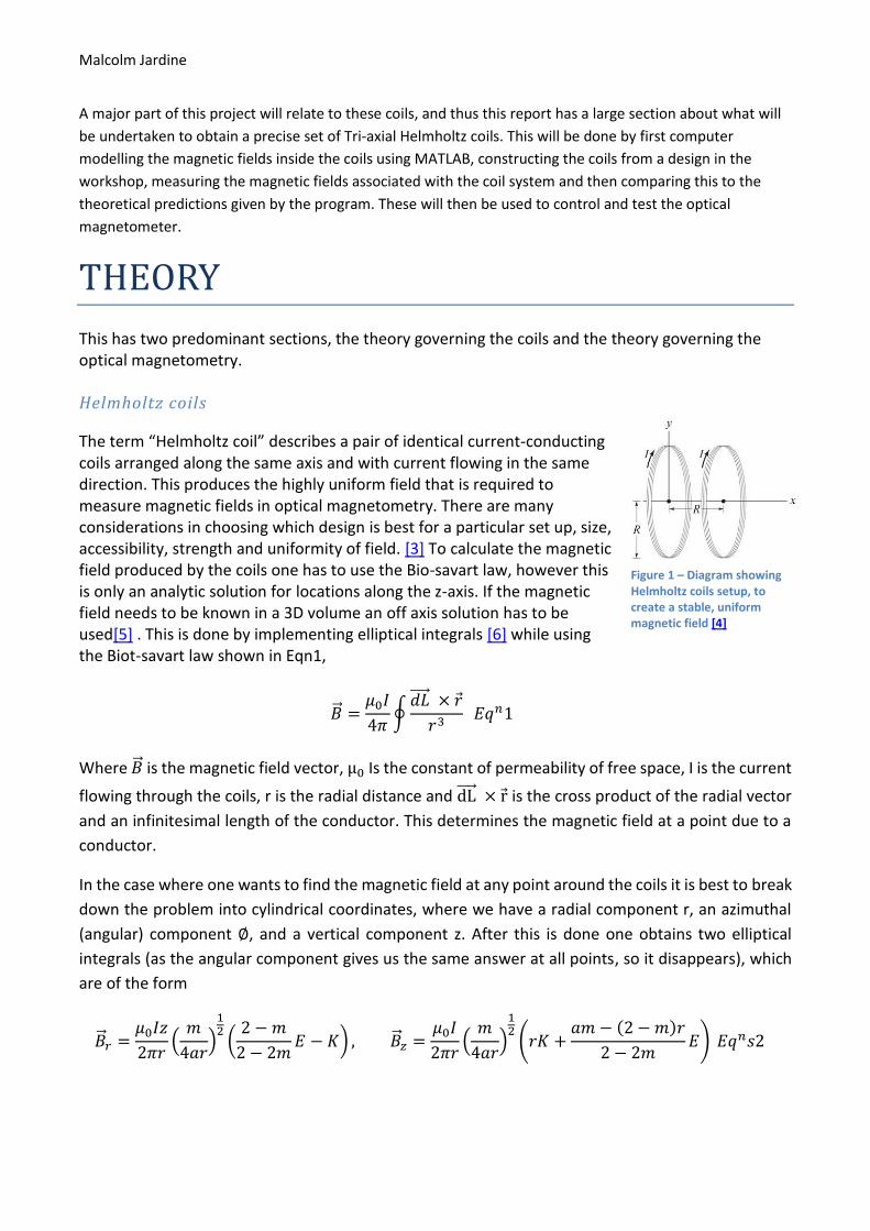
The term “Helmholtz coil” describes a pair of identical current-conducting coils arranged along the same axis and with current flowing in the same direction. This produces the highly uniform field that is required to measure magnetic fields in optical magnetometry. There are many considerations in choosing which design is best for a particular set up, size, accessibility, strength and uniformity of field. [3] To calculate the magnetic field produced by the coils one has to use the Bio-savart law, however this is only an analytic solution for locations along the z-axis. If the magnetic field needs to be known in a 3D volume an off axis solution has to be used[5] . This is done by implementing elliptical integrals [6] while using the Biot-savart law shown in Eqn1,

�⃗� =𝜇0𝐼

4𝜋∮

𝑑𝐿⃗⃗⃗⃗ × 𝑟

𝑟3 𝐸𝑞𝑛1

Where �⃗� is the magnetic field vector, μ0 Is the constant of permeability of free space, I is the current

flowing through the coils, r is the radial distance and dL⃗⃗⃗⃗ × r is the cross product of the radial vector

and an infinitesimal length of the conductor. This determines the magnetic field at a point due to a

conductor.

In the case where one wants to find the magnetic field at any point around the coils it is best to break

down the problem into cylindrical coordinates, where we have a radial component r, an azimuthal

(angular) component ∅, and a vertical component z. After this is done one obtains two elliptical

integrals (as the angular component gives us the same answer at all points, so it disappears), which

are of the form

�⃗� 𝑟 =𝜇0𝐼𝑧

2𝜋𝑟(

𝑚

4𝑎𝑟)

12(

2 − 𝑚

2 − 2𝑚𝐸 − 𝐾) , �⃗� 𝑧 =

𝜇0𝐼

2𝜋𝑟(

𝑚

4𝑎𝑟)

12(𝑟𝐾 +

𝑎𝑚 − (2 − 𝑚)𝑟

2 − 2𝑚𝐸) 𝐸𝑞𝑛𝑠2

Figure 1 – Diagram showing Helmholtz coils setup, to create a stable, uniform magnetic field [4]

Malcolm Jardine

Where B⃗⃗ r is the radial component of the magnetic field; B⃗⃗ z is the vertical component of the magnetic

field; a is the radius of the coil; m is known as the elliptical parameter and it describes how the

elliptical integrals behave in a certain geometry and E and K are elliptical integrals of the first and

second kind. These can be calculated very quickly and accurately in mathematical programs such as

MATLAB, so one is able to calculate the magnetic field at each point in a 3D coordinate system using

these equations. These magnetic field components can then be transformed back into normal x,y,z

Cartesian coordinates which would be more useful in a set up that contained the coils. The Helmholtz

coils configuration to be calculated here uses this method, but has coils of six different orientations,

sizes, currents etc. and is tackled in the methodology in the report when discussing MATLAB.

MATLAB was also used to create a useful program which was an Analytic linear fitting function.

Instead of using excel or MATLAB’s iterative methods of finding a linear fit a program was

developed that analytically minimises the Chi-squared value. It is an analytic solution to the linear

regression chi squared method, and it used the function

Χ2 = ∑1

𝜎𝑖

𝑁

𝑖

(𝑦𝑖 − 𝑐 − 𝑚𝑥𝑖)

where 𝑦𝑖 is the experimentally measured data point, 𝑥𝑖 is the x-axis data point, 𝜎𝑖 is the uncertainty

in each 𝑦𝑖 data point and m and c are the gradient and y intercept respectively of a linear fit. The

objective of this Chi-squared test is to reduce the difference of each point between the linear fit and

the actual experimental data. Solving this and using a system of equations gives us the exact value of

m, c, the uncertainties associated with both of these derived parameters and some other statistics,

such as the residuals. Whereas most computer programs just minimise this Chi-squared value by

‘guessing’ many times, this method provides an analytic value for the linear fit.

Optical magnetometry

This is the use of lasers to determine magnetic fields. There are many different methods and

procedures to achieve this, but they all work on similar principles. The basic principle is using

coherent, polarised light and the atomic spin states of the alkali vapour that are optically pumped

to a higher state until no more absorption of the photons take place. Then an applied oscillating

magnetic field (Known as BAC as it is an alternating magnetic field produced by an alternating

current) causes these states to undergo Larmor precession where they come back down to an

absorption state. This affects the amount of light being absorbed which can be detected.

In order to understand the fundamental principles of optical magnetometers, it is first useful to consider the energy structure of an alkali-metal atom. This is dictated by quantum physics, but the important point is the energy difference in the energy levels of atoms and electrons and how they change under an applied magnetic field.

Malcolm Jardine

In atomic emission and absorption spectroscopy the different energy levels arise from the different energy levels an electron can occupy in the atomic structure. This is shown in figure 2. The S and P are notation for the different energy levels The atomic structure goes much deeper than this. One sees at first, as is the case with figure 2, there are the transitions on what is called the

fine structure, which involve the available sites for the electron to occupy and its spin. However the transitions that are used in the optical magnetometers use a more complicated set of quantum numbers which concern the interaction of the spin of the nucleus and the orbital angular momentum of the electrons. This is what makes the hyperfine structure which behaves, for the S1/2 state, as shown in figure 3

This now shows the hyperfine structure with

different energy states. This splitting of the S1/2

or P1/2 splits it into two different states, the

higher energy levels, such as P3/2, split into a

larger number of states.

Again there is more happening here that one needs to consider, as with the application of a small magnetic field (these F states split again), this is demonstrated in figure 4

The numbers that label the Zeeman Splitting describe the electron’s projection of its orbital angular momentum which affects its energy. The energy states that are of interest here are one in higher momentum states, where the transitions that are of concern are F=4 and F=3. The equations describing the absorption of these states are well understood, and applying a small magnetic field causes the system to deviate from these equations by a small amount. A Taylor expansion is then used around this point, which is of the form of a lorentzian curve, which can then be used to

S1/2

P1/2

Figure 2 – The jump of an electron from the S orbit to the P orbit which is in the fine structure. The lines represent energy levels and the arrow represents an electron being elevated to a higher energy level at the cost of absorbing a photon of the correct energy.

S1/2

F=1

F=2

Figure 3 – the splitting of the S orbit due to the interaction of electrons with the spin of the nucleus. This is the hyperfine structure.

S1/2

F=1

F=2

2 1 0 -1 -2 1 0 -1

Fine Structure Hyperfine Structure Zeeman Splitting

Figure 4 – further splitting of the available energy states due to an applied magnetic field, these are the states that are optically pumped.

Malcolm Jardine

calculate the magnetic field. What is important is that the absorption by these states is not the same for different polarisations of light. The next step for the optical magnetometry is the optical pumping of these states. Photons are used to elevate the electrons to a higher energy state, and through a process of absorption and spontaneous emission, eventually all the electrons are in their highest available energy state, and thus stop absorbing light. However, with the application of the BAC field, these states become depopulated as the electrons fall back down to the absorptive states, thus absorbing more light. If the transmission of the laser is monitored then the applied magnetic field can be calculated, as the rate of precession of the states in the BAC field is related to the magnetic field. [7] There are several limitations associated with optical pumping: these can be with spin-exchange interactions when two atoms collide; or when the spin states are randomly depolarised (i.e. lose their ‘dark’ states) and when they collide with the wall of the cell. These processes all cause the atoms to come out of the dark state such that they cannot be used for measurement. These limitations can be suppressed by the use of a buffer gas, such as N2, or by the use of an anti-relaxation coating on the inside of the gas cell, such as paraffin. These increase the coherence time and thus a longer measurement of the Larmor procession can be made and a better result obtained.

Methodology

MATLAB A large proportion of what was undertaken in the placement was the use of MATLAB to design an

application package to calculate and manipulate the magnetic field produced in the Tri-axial

Helmholtz coil system; this was done using a MATLAB Graphical User Interface (GUI).

First one had to download a code from online that made use of the Biot-savart law and

several approximations to calculate the magnetic field for a conducting ring, i.e. a singular coil. The

use of the elliptical integrals, which are inbuilt in MATLAB, were then implemented to provide a

more accurate result. This was done for all six coils so one could calculate the three magnetic field

components, Bx, By and Bz, in the volume enclosed by the coils. This was all implemented in a

multifunctional, highly controllable GUI package which was designed to be able to do the following:

change all the parameters of each of the coils; control the precision and volume over which the

field was calculated; plot a 3D surface to demonstrate the shape of the produced magnetic field;

investigate the magnetic field and magnetic field gradient along any axis in the coils; to plot the

uniformity of the field over any plane and to be able to save the data from any of these functions

for further inspection.

Additionally the analytic linear fitting function was designed, which was then improved in order to

handle uncertainties with both the yI and xi data points and return the R2 for the fitted data.

Malcolm Jardine

Tri-axial Helmholtz coils Initially each of the 6 coils had to be wound using copper wire to given specifications which are

given in table 1 in the appendix. These were found using Eqn1 to determine the magnitude of the

field produced by each coil (which had to be chosen to either be able to compensate for the earth’s

magnetic field or produce a field vector that the optical magnetometers could measure), and also

the derivative of Eqn1 to work out the field gradients produced by the coils. This was important as

the field gradient affected the width of our measured transitions which in turn affects the

sensitivity of the optical magnetometer.

They were then assembled in the Tri-axial set up as shown in

figure 5 and tested. This was done using a fluxgate

magnetometer and placing it inside the coils at known locations

and taking values of the magnetic field. This was then compared

quantitavely to the expected results from the specifications and

from the calculations from the MATLAB GUI.

The two important results that had to be obtained were the

response of the magnetic field to a change in current (B/I) while

holding the distance constant at the centre of the coils; and the

response of the magnetic field while changing the distance at a

constant value of current (B/I/m). The two test procedures

below were performed for all 3 sets of the coils individually.

To determine the B/I one had to first determine the

centre point of the coils. This was done by first placing the coils in the anti-Helmholtz (AH)

configuration and finding where the magnetic field was 0 due to the coils (figure 7 displays how the

magnetic field changes as one travels through the centre of the coils in AH configuration). The

magnetometer was then held here and the values of the magnetic field were taken as a function of

changing current to find the B/I result. The current range that was used was -1A to 1A, as within

this range the coils were able create a field with a magnitude of that of the earth’s field. This

procedure was performed for all three coils.

To find B/I/m one performed the same operation as the initial tests where the magnetic

field was tested for set locations in a line through the centre of the coils while holding the current

constant. This was done in the Helmholtz configuration. However this result is only linear in a small

region in the centre, so the magnetometer was only moved by a distance of about 20% of the radii

of the coils along the centre.

Optical Magnetometry To find the F4 to F3 transitions (D1 line in caesium) the setup shown in figure 6 was used. Using a

highly stable External Cavity Diode Laser (ECDL) the laser first had to be configured to a reference

caesium cell and the beam calibrated and monitored using an oscilloscope. The purpose of this was

to achieve a ‘clean’ beam with no feedback and to be ‘locked on’ to the correct frequency of the

Figure 5 – Isometric view of the assembled Tri-axial Helmholtz coils with one stand in place - specifications are given in table one in the appendix

Malcolm Jardine

atomic transitions that was being used in the optical magnetometry. The beam was then coupled to

a fibre (using the beam splitter to split the beam between the optical magnetometer and the

calibration setup) to be used to probe the 2nd caesium gas vapour cell.

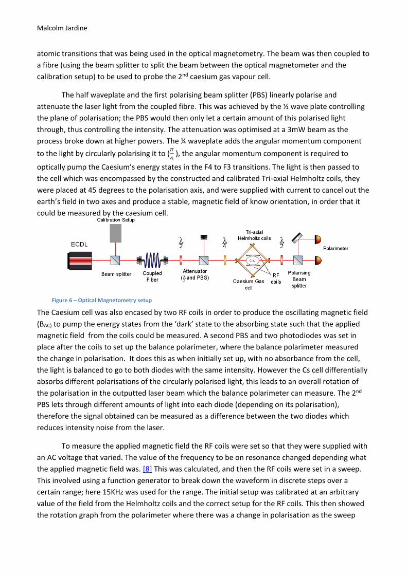
The half waveplate and the first polarising beam splitter (PBS) linearly polarise and

attenuate the laser light from the coupled fibre. This was achieved by the ½ wave plate controlling

the plane of polarisation; the PBS would then only let a certain amount of this polarised light

through, thus controlling the intensity. The attenuation was optimised at a 3mW beam as the

process broke down at higher powers. The ¼ waveplate adds the angular momentum component

to the light by circularly polarising it to (𝜋

4 ), the angular momentum component is required to

optically pump the Caesium’s energy states in the F4 to F3 transitions. The light is then passed to

the cell which was encompassed by the constructed and calibrated Tri-axial Helmholtz coils, they

were placed at 45 degrees to the polarisation axis, and were supplied with current to cancel out the

earth’s field in two axes and produce a stable, magnetic field of know orientation, in order that it

could be measured by the caesium cell.

The Caesium cell was also encased by two RF coils in order to produce the oscillating magnetic field

(BAC) to pump the energy states from the ‘dark’ state to the absorbing state such that the applied

magnetic field from the coils could be measured. A second PBS and two photodiodes was set in

place after the coils to set up the balance polarimeter, where the balance polarimeter measured

the change in polarisation. It does this as when initially set up, with no absorbance from the cell,

the light is balanced to go to both diodes with the same intensity. However the Cs cell differentially

absorbs different polarisations of the circularly polarised light, this leads to an overall rotation of

the polarisation in the outputted laser beam which the balance polarimeter can measure. The 2nd

PBS lets through different amounts of light into each diode (depending on its polarisation),

therefore the signal obtained can be measured as a difference between the two diodes which

reduces intensity noise from the laser.

To measure the applied magnetic field the RF coils were set so that they were supplied with

an AC voltage that varied. The value of the frequency to be on resonance changed depending what

the applied magnetic field was. [8] This was calculated, and then the RF coils were set in a sweep.

This involved using a function generator to break down the waveform in discrete steps over a

certain range; here 15KHz was used for the range. The initial setup was calibrated at an arbitrary

value of the field from the Helmholtz coils and the correct setup for the RF coils. This then showed

the rotation graph from the polarimeter where there was a change in polarisation as the sweep

Figure 6 – Optical Magnetometry setup

Malcolm Jardine

passed over the resonance frequency of the Caesium transmission line.

The graph that is produced by taking the difference of the two voltages from the two

photodiodes was fitted by a Lorentzian curve and the resulting parameters gave the value of the

applied magnetic field.

To test the sensitivity and reliability of the optical magnetometer it was tested against one of the

Tri-axial Helmholtz coils, the largest one. It was used to measure the magnetic field per amp and

compare it to the magnetometer result from before. This was done by changing the current value

for the largest Helmholtz coils, assigning the correct values for the RF coils with the same 15KHz

range and then obtaining the Lorentzian to work out the magnetic field at each value of current.

Results and Discussion

In doing this summer placement several useful MATLAB files were designed and produced, such as

an analytic linear fitting model and the Tri-axial Helmholtz coils application. These can be of further

use in the Quantum Optics labs and in my studies.

The first test results from the flux gate magnetometer to test the coils is shown in figure A in the

appendix. This was to demonstrate that the GUI theoretical calculations were correct compared to

the actual magnetometer data, since the theory and experiment are in good agreement (from

figure A). One could say the GUI is a good predictor of the magnetic field of a set of Tri-axial

Helmholtz coils. The small deviations are explainable by the imperfections in the windings of the

coils and in the width of the copper wires.

The two important results that had to be obtained for controlling the Helmholtz coils were the

response of the magnetic field while changing the distance at a constant value of current (B/I/m)

and the response of the magnetic field while changing the current at a point at the centre of the

coils (B/I). To find both these parameters for the three sets of coils the analytic linear fitting model

was used, where the results of the program are displayed in Table B in the index.

To find the gradient of the B-field response with respect

to small displacements (B/I/m) one had to first determine

where the approximately linear region is, this is displayed

in figure 7. This is because at the edges of the

measurement volume (so near the coils) the magnetic

field can be seen to be no longer approximately linear. So

to find this value for each of the coils one stayed in this

region. There was some magnetometer data taken in this

region to confirm the approximately linear relationship

with distance and magnetic field. This was done for all

three coils, with the gradient being taken from three

-50 0 50 Position [mm] along X-axis

By[

µT]

-6

0

0

-6

0

Figure 7 - This is the GUI plot of the magnetic field while moving along the X axis from the centre of one coil to the other. One can note that the line is approximately linear in the region around the centre, roughly 20mm out

Malcolm Jardine

separate figures, the one for the middle coil being shown in figure 8.

The gradient of the green fitted line (using

the developed fitting software) was

(1269 ± 10)µT/A/m. This compared well to

the desired result when building the coils: it

is only 5% from the specification in table 1.

However, if the plot is examined more

closely, by plotting the residuals (i.e. the

difference between each data point and the

fitted line) one would expect to see a

pattern as the fit is linear, but the

relationship is only approximately linear.

This closer inpection and residual plot is

shown in the residual graph of figure 9. One

can see how there is a pattern in the residuls

for the experimental data. To investigate this

the same residual plot was made for the

theoretical GUI data. This is figure B in the

appendix, which demonstrates the same

pattern in the residuals when a linear fit

(using the same analytic fitting program) is

applied to it, i.e. that the linear fit is truly only

an approximation at this resoltuion.

However what one is actually measuring is

the derivative field, and one actually wants

this value at the centre of the coils. So the

actual value become more exact the closer

one gets to an infintesmal step value around

the centre (like differntiation), however this

isn’t possible for accuarcy reasons so as such

one must make a linear approximation over a

small area and then obtainthe pattern.

The next step was to measure the response of

the magnetic field while changing the current

and holding the magnetometer at a point at

the centre of the coils (B/I). This result is

Position [mm] along the X axis

Figure 8 - The B/I/m measurement of the middle coil, this uses the analytic fitting program developed here to plot the line of best fit (green line) with given uncertainties from the data (red circles). This was taken over 25mm around the centre in the AH configuration

-20 -15 -10 -5 0 5 10 15

Position [mm] along X axis

Mag

nit

ud

e o

f re

sid

ual

Figure 9 – This is the residuals of figure 8. There is a clear pattern here, one that is a polynomial of some power, in the magnitude of the residuals. This implies that the linear fit is not the best one, and that a different fir would provide a more accurate description here.

Figure 10 – The gradient of the fitted line gives the B/I result for the largest coil where the magnetometer was held in the middle of the coils while changing the current and measuring the magnetic field.

Malcolm Jardine

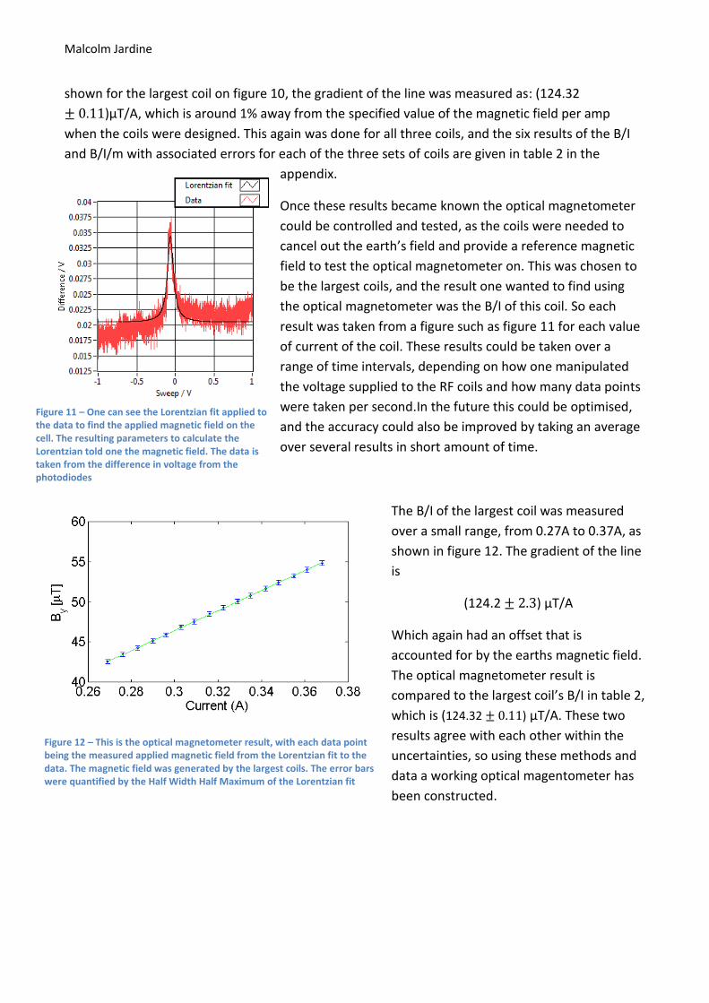
shown for the largest coil on figure 10, the gradient of the line was measured as: (124.32

± 0.11)μT/A, which is around 1% away from the specified value of the magnetic field per amp

when the coils were designed. This again was done for all three coils, and the six results of the B/I

and B/I/m with associated errors for each of the three sets of coils are given in table 2 in the

appendix.

Once these results became known the optical magnetometer

could be controlled and tested, as the coils were needed to

cancel out the earth’s field and provide a reference magnetic

field to test the optical magnetometer on. This was chosen to

be the largest coils, and the result one wanted to find using

the optical magnetometer was the B/I of this coil. So each

result was taken from a figure such as figure 11 for each value

of current of the coil. These results could be taken over a

range of time intervals, depending on how one manipulated

the voltage supplied to the RF coils and how many data points

were taken per second.In the future this could be optimised,

and the accuracy could also be improved by taking an average

over several results in short amount of time.

The B/I of the largest coil was measured

over a small range, from 0.27A to 0.37A, as

shown in figure 12. The gradient of the line

is

(124.2 ± 2.3) μT/A

Which again had an offset that is

accounted for by the earths magnetic field.

The optical magnetometer result is

compared to the largest coil’s B/I in table 2,

which is (124.32 ± 0.11) μT/A. These two

results agree with each other within the

uncertainties, so using these methods and

data a working optical magentometer has

been constructed.

Figure 11 – One can see the Lorentzian fit applied to the data to find the applied magnetic field on the cell. The resulting parameters to calculate the Lorentzian told one the magnetic field. The data is taken from the difference in voltage from the photodiodes

Figure 12 – This is the optical magnetometer result, with each data point being the measured applied magnetic field from the Lorentzian fit to the data. The magnetic field was generated by the largest coils. The error bars were quantified by the Half Width Half Maximum of the Lorentzian fit

Malcolm Jardine

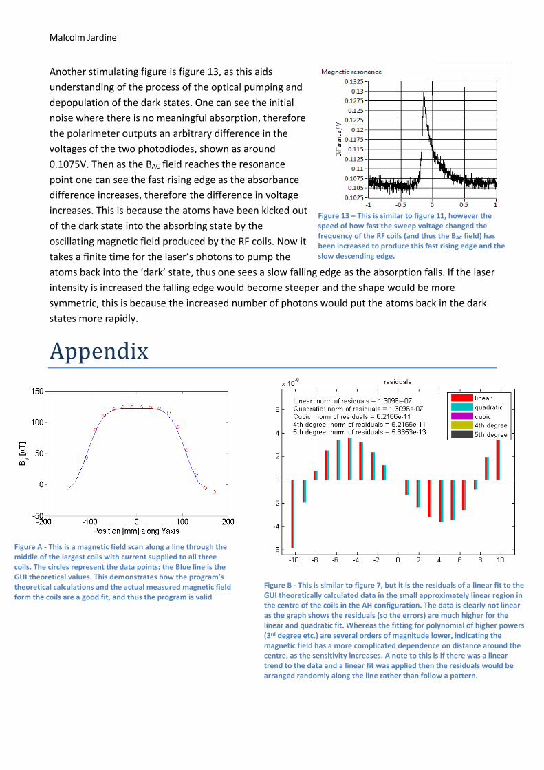
Another stimulating figure is figure 13, as this aids

understanding of the process of the optical pumping and

depopulation of the dark states. One can see the initial

noise where there is no meaningful absorption, therefore

the polarimeter outputs an arbitrary difference in the

voltages of the two photodiodes, shown as around

0.1075V. Then as the BAC field reaches the resonance

point one can see the fast rising edge as the absorbance

difference increases, therefore the difference in voltage

increases. This is because the atoms have been kicked out

of the dark state into the absorbing state by the

oscillating magnetic field produced by the RF coils. Now it

takes a finite time for the laser’s photons to pump the

atoms back into the ‘dark’ state, thus one sees a slow falling edge as the absorption falls. If the laser

intensity is increased the falling edge would become steeper and the shape would be more

symmetric, this is because the increased number of photons would put the atoms back in the dark

states more rapidly.

Appendix

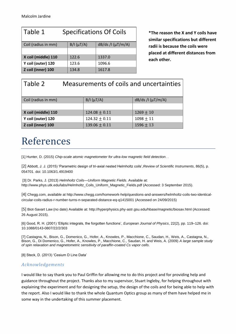
Figure A - This is a magnetic field scan along a line through the middle of the largest coils with current supplied to all three coils. The circles represent the data points; the Blue line is the GUI theoretical values. This demonstrates how the program’s theoretical calculations and the actual measured magnetic field form the coils are a good fit, and thus the program is valid

Figure B - This is similar to figure 7, but it is the residuals of a linear fit to the GUI theoretically calculated data in the small approximately linear region in the centre of the coils in the AH configuration. The data is clearly not linear as the graph shows the residuals (so the errors) are much higher for the linear and quadratic fit. Whereas the fitting for polynomial of higher powers (3rd degree etc.) are several orders of magnitude lower, indicating the magnetic field has a more complicated dependence on distance around the centre, as the sensitivity increases. A note to this is if there was a linear trend to the data and a linear fit was applied then the residuals would be arranged randomly along the line rather than follow a pattern.

Figure 13 – This is similar to figure 11, however the speed of how fast the sweep voltage changed the frequency of the RF coils (and thus the BAC field) has been increased to produce this fast rising edge and the slow descending edge.

Malcolm Jardine

References

[1] Hunter, D. (2015) Chip-scale atomic magnetometer for ultra-low magnetic field detection. .

[2] Abbott, J. J. (2015) ‘Parametric design of tri-axial nested Helmholtz coils’,Review of Scientific Instruments, 86(5), p.

054701. doi: 10.1063/1.4919400

[3] Dr. Parks, J. (2013) Helmholtz Coils—Uniform Magnetic Fields. Available at:

http://www.phys.utk.edu/labs/Helmholtz_Coils_Uniform_Magnetic_Fields.pdf (Accessed: 3 September 2015).

[4] Chegg.com, available at http://www.chegg.com/homework-help/questions-and-answers/helmholtz-coils-two-identical-

circular-coils-radius-r-number-turns-n-separated-distance-eq-q1415001 (Accessed on 24/09/2015)

[5] Biot-Savart Law (no date) Available at: http://hyperphysics.phy-astr.gsu.edu/hbase/magnetic/biosav.html (Accessed:

26 August 2015).

[6] Good, R. H. (2001) ‘Elliptic integrals, the forgotten functions’, European Journal of Physics, 22(2), pp. 119–126. doi:

10.1088/0143-0807/22/2/303

[7] Castagna, N., Bison, G., Domenico, G., Hofer, A., Knowles, P., Macchione, C., Saudan, H., Weis, A., Castagna, N., Bison, G., Di Domenico, G., Hofer, A., Knowles, P., Macchione, C., Saudan, H. and Weis, A. (2009) A large sample study of spin relaxation and magnetometric sensitivity of paraffin-coated Cs vapor cells. [8] Steck, D. (2013) ‘Cesium D Line Data’

Acknowledgements

I would like to say thank you to Paul Griffin for allowing me to do this project and for providing help and

guidance throughout the project. Thanks also to my supervisor, Stuart Ingleby, for helping throughout with

explaining the experiment and for designing the setup, the design of the coils and for being able to help with

the report. Also I would like to thank the whole Quantum Optics group as many of them have helped me in

some way in the undertaking of this summer placement.

Table 1 Specifications Of Coils

Coil (radius in mm) B/I (µT/A) dB/ds /I (µT/m/A)

X coil (middle) 110 122.6 1337.0

Y coil (outer) 120 123.6 1096.6

Z coil (inner) 100 134.8 1617.8

Table 2 Measurements of coils and uncertainties Coil (radius in mm) B/I (µT/A) dB/ds /I (µT/m/A)

X coil (middle) 110 124.08 ± 0.11 1269 ± 10

Y coil (outer) 120 124.32 ± 0.11 1098 ± 11

Z coil (inner) 100 139.06 ± 0.11 1596 ± 13

*The reason the X and Y coils have

similar specifications but different

radii is because the coils were

placed at different distances from

each other.