arX

iv:1

302.

4793

v2 [

cs.N

I] 1

2 Ju

l 201

3

Opportunistic Wireless Energy Harvesting inCognitive Radio Networks

Seunghyun Lee, Rui Zhang,Member, IEEE, and Kaibin Huang,Member, IEEE

Abstract—Wireless networks can be self-sustaining by harvest-ing energy from ambient radio-frequency (RF) signals. Recently,researchers have made progress on designing efficient circuits anddevices for RF energy harvesting suitable for low-power wirelessapplications. Motivated by this and building upon the classiccognitive radio (CR) network model, this paper proposes a novelmethod for wireless networks coexisting where low-power mobilesin a secondary network, called secondary transmitters (STs),harvest ambient RF energy from transmissions by nearby activetransmitters in a primary network, called primary transmitters(PTs), while opportunistically accessing the spectrum licensedto the primary network. We consider a stochastic-geometrymodel in which PTs and STs are distributed as independenthomogeneous Poisson point processes (HPPPs) and communicatewith their intended receivers at fixed distances. Each PT isassociated with a guard zone to protect its intended receiverfrom ST’s interference, and at the same time delivers RF energyto STs located in its harvesting zone. Based on the proposedmodel, we analyze the transmission probability of STs andthe resulting spatial throughput of the secondary network.Theoptimal transmission power and density of STs are derived formaximizing the secondary network throughput under the givenoutage-probability constraints in the two coexisting networks,which reveal key insights to the optimal network design. Finally,we show that our analytical result can be generally applied toa non-CR setup, where distributed wireless power chargers aredeployed to power coexisting wireless transmitters in a sensornetwork.

Index Terms—Cognitive radio, energy harvesting, opportunis-tic spectrum access, wireless power transfer, stochastic geometry.

I. I NTRODUCTION

POwering mobile devices by harvesting energy from am-bient sources such as solar, wind, and kinetic activities

makes wireless networks not only environmentally friendlybut also self-sustaining. Particularly, it has been reportedin the recent literature that harvesting energy from ambientradio-frequency (RF) signals can power a network of low-power devices such as wireless sensors [1]–[6]. In theory, themaximum power available for RF energy harvesting at a free-space distance of40 meters is known to be7uW and1uWfor 2.4GHz and 900MHz frequency, respectively [2]. Mostrecently, Zungeruet al. have achieved harvested power of3.5mW at a distance of0.6 meter and1uW at a distance of11 meters using Powercast RF energy-harvester operating at

S. Lee and R. Zhang are with the Department of Electrical and ComputerEngineering, National University of Singapore, Singapore(email: {elelees,elezhang}@nus.edu.sg). R. Zhang is also with the Institute for InfocommResearch, A*STAR, Singapore.

K. Huang is with the Department of Applied Mathematics, HongKongPolytechnic University, Hong Kong (email: huangkb@ieee.org).

915MHz [2]. It is expected that more advanced technologiesfor RF energy harvesting will be available in the near futuredue to e.g. the rapid advancement in designing highly efficientrectifying antennas [3].

In this work, we investigate the impact of RF energyharvesting on the newly emerging cognitive radio (CR) typeof networks. To this end, we propose a novel method forwireless networks coexisting where transmitters from a sec-ondary network, calledsecondary transmitters (STs), eitheropportunistically harvest RF energy from transmissions bynearby transmitters from a primary network, or transmit sig-nals if theseprimary transmitters (PTs) are sufficiently faraway. STs store harvested energy in rechargeable batterieswith finite capacity and apply the available energy for sub-sequent transmissions when batteries are fully charged. Thethroughput of the secondary network is analyzed based ona stochastic-geometry model, where the PTs and STs aredistributed according to independent homogeneous Poissonpoint processes (HPPPs). In this model, each PT is assumedto randomly access the spectrum with a given probabilityand each active (transmitting) PT is centered at aguardzone as well as aharvesting zone that is inside the guardzone. As a result, each ST harvests energy if it lies in theharvesting zone of any active PT, or transmits if it is outsidethe guard zones of all active PTs, or is idle otherwise. Thismodel is applied to maximize the spatial throughput of thesecondary network by optimizing key parameters including theST transmit power and density subject to given PT transmitpower and density, guard/harvesting zone radius, and outage-probability constraints in both the primary and secondarynetworks.

Our work is motivated by a joint investigation of theproposed conventionalopportunistic spectrum access and thenewly introducedopportunistic energy harvesting in CR net-works, i.e., during the idle time of STs due to the presence ofnearby active PTs, they can take such an opportunity to harvestsignificant RF energy from primary transmissions. Specifically,as shown in Fig. 1, each ST can be in one of the followingthree modes at any given time:harvesting mode if it is insidethe harvesting zone of an active PT and not fully charged;transmitting mode if it is fully charged and outside the guardzone of all active PTs; andidle mode if it is fully chargedbut inside any of the guard zones, or neither fully charged norinside any of the harvesting zones.

A. Related Work

Recently, wireless communication powered by energy har-vesting has emerged to be a new and active research area.

2

PT: Transmitting

ST: Transmitting

ST: Idle (fully charged)

ST: Harvesting

ST: Idle

(not fully charged)

Harvesting zone

Guard zone

rgrhr

PT: Idle

Fig. 1. A wireless energy harvesting CR network in which PTs and STs aredistributed as independent HPPPs. Each PT/ST has its intended informationreceiver at fixed distances (not shown in the figure for brevity). ST harvestsenergy from a nearby PT if it is inside its harvesting zone. Toprotect theprimary transmissions, ST inside a guard zone is prohibitedfrom transmission.

However, due to energy harvesting, existing transmissionalgorithms for conventional wireless systems with constantpower supplies (e.g., batteries) need to be redesigned toaccount for the new challenges such as random energy ar-rivals. For point-to-point wireless systems powered by energyharvesting, the optimal power-allocation algorithms havebeendesigned and shown to follow modified water-filling by Hoand Zhang [7] and Ozelet al. [8]. From a network perspective,Huang investigated the throughput of a mobile ad-hoc network(MANET) powered by energy harvesting where the networkspatial throughput is maximized by optimizing the transmitpower level under an outage constraint [9]. Furthermore, theperformance of solar-powered wireless sensor/mesh networkshas been analyzed in [10], in which various sleep and wakeupstrategies are considered.

Among other energy scavenging sources such as solar andwind, background RF signals can be a viable new sourcefor wireless energy harvesting [11]. A new research trendon wireless power transfer is to integrate this technologywith wireless communication. In [12] and [13], simultaneouswireless power and information transfer has been investigated,aiming at maximizing information rate and transferred powerover single-antenna additive white Gaussian noise (AWGN)channels. For broadcast channels, Zhang and Ho have studiedmulti-antenna transmission for simultaneous wireless informa-tion and power transfer with practical receiver designs such astime switching and power splitting [14]. Moreover, Zhouet al.have proposed a new receiver design for enabling wirelessinformation and power transmission at the same time, byjudiciously integrating conventional information and energyreceivers [15]. For point-to-point wireless systems, Liuetal. have studied “opportunistic” RF energy harvesting wherethe receiver opportunistically harvests RF energy or decodesinformation subject to time-varying co-channel interference[16]. More recently, Huang and Lau have proposed a newcellular network architecture consisting of power beacons

deployed to deliver wireless energy to mobile terminals andcharacterized the trade-off between the power-beacon densityand cellular network spatial throughput [17].

In another track, the emerging CR technology enablesefficient spectrum usage by allowing a secondary network toshare the spectrum licensed to a primary network withoutsignificantly degrading its performance [18]. Besides activedevelopment of algorithms for opportunistic transmissions bysecondary users (see e.g. [19], [20] and references therein),notable research has been pursued on characterizing thethroughput of coexisting wireless networks based on the toolof stochastic geometry. For example, the capacity trade-offsbetween two or more coexisting networks sharing a commonspectrum have been studied in [21]–[23]. Moreover, the outageprobability of a Poisson-distributed CR network with guardzones has been analyzed by Lee and Haenggi [24], where thesecondary users opportunistically access the primary users’channel only when they are not inside any of the guard zones.

B. Summary and Organization

In this paper, we consider a CR network with time slottedtransmissions and PT/ST locations modeled by independentHPPPs. The ST transmission power is assumed to be suf-ficiently small to meet the low-power requirement with RFenergy harvesting. Under this setup, the main results of thispaper are summarized as follows:

1) We propose a new CR network architecture whereSTs are powered by harvesting RF energy from activeprimary transmissions. We study the ST transmissionprobability as a function of ST transmit power in thepresence of both guard zones and harvesting zones basedon a Markov chain model. For the cases of single-slot and double-slot charging, we obtain the expressionsof the exact ST transmission probability, while for thegeneral case of multi-slot charging with more than twoslots, we obtain the upper and lower bounds on the STtransmission probability.

2) With the result of ST transmission probability, we derivethe outage probabilities of coexisting primary and sec-ondary networks subject to their mutual interferences,based on stochastic geometry and a simplified assump-tion on the HPPP of transmitting STs with an effectivedensity equal to the product of the ST transmission prob-ability and the ST density. Furthermore, we maximizethe spatial throughput of the secondary network undergiven outage constraints for the coexisting networksby jointly optimizing the ST transmission power anddensity, and obtain simple closed-form expressions ofthe optimal solution.

3) Furthermore, we show that our analytical result can begenerally applied to even non-CR setups, where dis-tributed wireless power chargers (WPCs) are deployedto power coexisting wireless information transmitters(WITs) in a sensor network, as shown in Fig. 2.Practically, WPCs can be implemented as e.g.wirelesscharging vehicles [25], or fixed power beacons [17]randomly deployed in a wireless sensor network. Based

3

WPC: Transmitting

WIT: Transmitting

WIT: Harvesting

WIT: Idle

(not fully charged)

Harvesting zone

rh

Fig. 2. A wireless powered sensor network in which WPCs and WITs aredistributed as independent HPPPs. Each WIT has intended receiver at a fixeddistance (not shown in the figure for brevity). WIT harvests energy from anearby WPC if inside its harvesting zone. Unlike the CR setupin Fig. 1, theguard zone is not applicable in this case, and thus a fully charged WIT cantransmit at any time.

on our result for the CR network setup, we derive themaximum network throughput of such wireless poweredsensor networks in terms of the optimal density andtransmit power of WITs.

The remainder of this paper is organized as follows. Sec-tion II describes the system model and performance metric.Section III analyzes the transmission probability of energy-harvesting STs. Section IV studies the outage probabilities inthe primary and secondary networks. Section V investigatesthe maximization of the secondary network throughput subjectto the primary and secondary outage probability constraints.Section VI extends the result to the wireless powered sensornetwork setup. Finally, Section VII concludes the paper.

II. SYSTEM MODEL

A. Network Model

As shown in Fig. 1, we consider a CR network in whichPTs and STs are distributed as independent HPPPs1 withdensityλ′

p andλs, respectively, withλ′

p ≪ λs. It is assumedthat time is slotted and each PT independently accesses thespectrum with probabilityp at each time slot. Thus, the pointprocess of active PTs forms another HPPP with densityλp =pλ′

p, according to the Coloring Theorem [28], which variesindependently over different slots. For convenience, we referto active PTs simply as PTs in the rest of this paper. Wedenote the point processes of PTs and STs asΦp = {X}and Φs = {Y }, respectively, whereX,Y ∈ R

2 denote thecoordinates of the PTs and STs, respectively. In addition, itis assumed that each PT/ST transmits with fixed power toits intended primary/secondary receiver (PR/SR) at distances

1In general, transmitters’ locations in cognitive radio networks may havenon-homogeneous or even non-Poisson spatial distributions, which are diffi-cult to characterize and not amenable to analysis. In this paper, we assumeHPPP for transmitters’ locations to obtain tractable analysis for the networkperformance.

dp andds, respectively, in random directions. We denote thefixed transmission power levels of PTs and STs asPp andPs,respectively. We assumePp ≫ Ps in this paper for energyharvesting applications of practical interest.

STs access the spectrum of the primary network and thustheir transmissions potentially interfere with PRs. To protectthe primary transmissions, STs are prevented from transmittingwhen they lie in any of theguard zones, modeled as diskswith a fixed radius centered at each PT. Specifically, letb(T, x) ⊂ R

2 represent a disk of radiusx centered atT ∈ R2;

then b(X, rg) denotes the guard zone with radiusrg forprotecting PTX ∈ Φp. DefineG =

⋃

X∈Φpb(X, rg) as the

union of all PTs’ guard zones; accordingly, an STY ∈ Φs

cannot transmit ifY ∈ G. Note that in practice the guardzone is usually centered at a PR rather than a PT as wehave assumed, while our assumption is made to simplify ouranalysis, similarly as in [19]. We further assumedp ≪ rgto guarantee that guard zones centered at PTs (rather thanPRs) will protect the primary transmissions properly. Underthe above assumptions, the probabilitypg that a typical ST,denoted byY ⋆, does not lie inG is equal to the probability thatthere is no PT inside the disk centered atY ⋆ with radiusrg,i.e., b(Y ⋆, rg). Note that the number of PTs insideb(Y ⋆, rg),denoted byN , is a Poisson random variable with meanπr2gλp;thus, its probability mass function (PMF) is given by

Pr{N = n} = e−πr2gλp(πr2gλp)

n

n!, n = 0, 1, 2, ... (1)

Consequently,pg can be obtained as

pg = Pr{Y ⋆ /∈ G} (2)

= Pr{N = 0} (3)

= e−πr2gλp . (4)

We assume flat-fading channels with path-loss and Rayleighfading; hence, the channel gains are modeled as exponentialrandom variables. As a result, in a particular time slot, thesignals transmitted from a PT/ST are received at the originwith powergXPp|X |−α andgY Ps|Y |−α, respectively, where{gX}X∈Φp

and {gY }Y ∈Φsare independent and identically

distributed (i.i.d.) exponential random variables with unitmean,α > 2 is the path-loss exponent, and|X |, |Y | denotethe distances from nodeX,Y to the origin, respectively.

B. Energy-Harvesting Model

To make use of the RF energy as an energy-harvestingsource, each RF energy harvester in an ST must be equippedwith a power conversion circuit that can extract DC powerfrom the received electromagnetic waves [1]. Such circuitsinpractice have certain sensitivity requirements, i.e., theinputpower needs to be larger than a predesigned threshold for thecircuit to harvest RF energy efficiently. This fact thus motivatesus to define theharvesting zone, which is a disk with radiusrh centered at each PTX ∈ Φp with rh ≪ rg. The radiusrh is determined by the energy harvesting circuit sensitivityfor a givenPp, such that only STs inside a harvesting zonecan receive power larger than the energy harvesting threshold,which is given byPpr

−αh . The power received by an ST

4

outside any harvesting zone is too small to activate the energyharvesting circuit, and thus is assumed to be negligible in thispaper.

Let b(X, rh) represent the harvesting zone centered at PTX ∈ Φp such that an STY can harvest energy from one ormore PTs ifY ∈ H, whereH =

⋃

X∈Φpb(X, rh) denotes the

union of the harvesting zones of all PTs. The probabilityphthat a typical STY ⋆ lies in H is equal to the probability thatthere is at least one PT inside the diskb(Y ⋆, rh). Similar to(1), the number of PTs insideb(Y ⋆, rh), denoted byK, is aPoisson random variable with meanπr2hλp and PMF given by

Pr{K = k} = e−πr2hλp(πr2hλp)

k

k!, k = 0, 1, 2, ... (5)

Accordingly,ph is given by

ph = Pr{Y ⋆ ∈ H} (6)

= Pr{K ≥ 1} (7)

=∞∑

k=1

e−πr2hλp(πr2hλp)

k

k!(8)

= 1− e−πr2hλp . (9)

Sinceλp and rh are both practically small, we can assumeπr2hλp ≪ 1. Thus,ph given in (8) can be approximated asPr{K = 1} by ignoring the higher-order terms withk > 1.Therefore, whenY ⋆ ∈ H, Y ⋆ is inside the harvesting zone ofone single PT most probably, which equivalently means thatthe harvesting zones of different PTs do not overlap at mosttime. As a result, the amount of average power harvested byY ⋆ ∈ H in a time slot can be lower-bounded byηPpR

−α

whereR ≤ rh denotes the distance betweenY ⋆ and its nearestPT, and0 < η < 1 denotes the harvesting efficiency. Note thatthe harvested power has been averaged over the channel short-term fading within a slot.

C. ST Transmission Model

We assume that each ST has a battery of finite capacityequal to the minimum energy required for one-slot transmis-sion with powerPs for simplicity. Upon the battery beingfully charged, an ST will transmit with all stored energy inthe next slot if it is outside all the guard zones. We denote theprobability thatY ⋆ has been fully charged at the beginningof a time slot aspf and the probability that it will be ableto transmit in this slot aspt. As mentioned above, the pointprocess of PTsΦp varies independently over different slots,and thus the events that an ST has been fully charged in oneslot and that it is outside all the guard zones in the next slotare independent. Consequently,pt can simply be obtained as

pt = pfpg, (10)

wherepg is given in (4), andpf will be derived in Section III.

D. Performance Metric

For both PRs and SRs, the received signal-to-interference-plus-noise ratio (SINR) is required to exceed a given targetfor reliable transmission. Letθp and θs be the target SINR

for the PR and SR, respectively. The outage probability isthen defined asP (p)

out= Pr{SINR(p) < θp} for the primary

network andP (s)out

= Pr{SINR(s) < θs} for the secondarynetwork. The outage-probability constraints are applied suchthatP (p)

out≤ ǫp andP (s)

out≤ ǫs with given0 < ǫp, ǫs < 1. Note

that the transmitting STs in general do not form an HPPPdue to the presence of guard zones and energy harvestingzones, but their average density over the network is given byptλs. Accordingly, given fixed PT densityλp and transmissionpowerPp, the performance metric of the secondary networkis the spatial throughputCs (bps/Hz/unit-area) given by

Cs = ptλs log2(1 + θs), (11)

under the given primary/secondary outage probability con-straintsǫp andǫs.

III. T RANSMISSION PROBABILITY OF SECONDARY

TRANSMITTERS

In this section, the transmission probability of a typical STpt given in (10) is analyzed using the Markov chain model. Forconvenience, we defineM as the maximum number of energy-harvesting time slots required to fully charge the battery of anST. Since the minimum power harvested by an ST in oneslot is ηPpr

−αh , which occurs when the ST is at the edge

of a harvesting zone, it follows thatM =⌈

Ps

ηPpr−α

h

⌉

, where

⌈x⌉ denotes the smallest integer larger than or equal tox.Note thatM = 1 corresponds to the case where the battery isfully charged within one slot time; thus this case is referredto as single-slot charging. Similarly, the case ofM = 2 isreferred to asdouble-slot charging. It will be shown in thissection that ifM = 1 or M = 2, the battery power levelcan be exactly modeled by a finite-state Markov chain; hence,the transmission probabilitypt can be obtained. However, formulti-slot charging with M > 2, only upper and lower boundson pt are obtained based on the Markov chain analysis for thecase ofM = 2.

A. Single-Slot Charging (M = 1)

If 0 < Ps ≤ ηPpr−αh , the battery of an ST is fully charged

within a slot, i.e.,M = 1. It thus follows that the batterypower level can only be either 0 orPs at the beginning ofeach slot. Consider the finite-state Markov chain with statespace{0, 1} with states0 and1 denoting the battery level ofpower 0 andPs, respectively. Furthermore, letP1 representthe state-transition probability matrix that can be obtained as

P1 =

[

1− ph phpg 1− pg

]

(12)

with pg and ph given in (4) and (9), respectively. Thenptcan be obtained by finding the steady-state probability of theassumed Markov chain, as given in the following proposition.

Proposition 3.1: If 0 < Ps ≤ ηPpr−αh or M = 1 (single-

slot charging), the transmission probability of a typical ST is

5

given by

pt =ph

ph + pgpg (13)

=(1 − e−πr2hλp)e−πr2gλp

1− e−πr2hλp + e−πr2gλp

. (14)

Proof: Let the steady-state probability of the two-stateMarkov chain be denoted byπ1 = [π1,0, π1,1], whereπ1 isthe left eigenvector ofP1 corresponding to the unit eigenvaluesuch that

π1P1 = π1. (15)

From (15), the steady-state distribution of the battery powerlevel at a typical ST is obtained as

π1,0 =pg

ph + pg, π1,1 =

phph + pg

. (16)

Note that the probability that an ST is fully charged at thebeginning of each slot as defined in (10) ispf = π1,1 in thiscase. Consequently, from (10), the desired result in (13) isobtained.

It is observed from (14) that in the single-slot charging case,pt depends only onλp, rh andrg, but is not related toPs. Thereason is that the battery of an ST is guaranteed to be fullycharged over one slot if it gets into a harvesting zone; hence,the probability that an ST is fully chargedpf = π1,1 = ph

ph+pg

does not depend onPs.

B. Double-Slot Charging (M = 2)

If ηPpr−αh < Ps ≤ 2ηPpr

−αh or M = 2, an ST needs

at most 2 slots of harvesting to make the battery fullycharged. To establish the Markov chain model for this case, wedivide the harvesting zoneb(X, rh) into two disjoint regions,

b(X,h1) and a(X,h1, rh), where h1 =(

Ps

ηPp

)−1α

< rh

and a(T, x, y) = b(T, y)\b(T, x) denotes the annulus withradii 0 < x < y centered atT ∈ R

2. It then follows thatthe regionb(X,h1) consists of the locations at which thepower harvested by a typical STY ⋆ from PT X is greaterthan or equal toPs (i.e., single-slot charging region), whilethe regiona(X,h1, rh) corresponds to the locations at whichthe power harvested byY ⋆ is greater than or equal to12Ps

but smaller thanPs (see Fig. 3). For convenience, we defineH1 =

⋃

X∈Φpb(X,h1) andH2 =

⋃

X∈Φpa(X,h1, rh). Note

that H = H1 ∪ H2. We reasonably assume thatH1 andH2

are disjoint since the harvesting zones are most likely disjointas mentioned in Section II-B.

Consider a 3-state Markov chain with state space{0, 1, 2}.Since the battery power level can only be either0 or in therange[ 12Ps, Ps] sinceηPpr

−αh ≥ 1

2Ps in this case, we definestate0 as the battery level of power 0, state1 with the powerlevel in the range[ 12Ps, Ps), and state2 with the power levelequal toPs. Note that in order to transit from state0 to 1,0 to 2, and 1 to 2, the harvested power atY ⋆ needs to be12Ps ≤ ηPpR

−α < Ps, ηPpR−α ≥ Ps, andηPpR

−α ≥ 12Ps,

respectively (or equivalentlyY ⋆ needs to be insideH2, H1,and H, respectively). Thanks to the fact that the minimumcharging power is always larger than or equal to1

2Ps in this

h1

rh

b(X,h1)

a(X,h1, rh)

X

Fig. 3. Divided harvesting zone for the case of double-slot charging (M = 2).

case, we can determine the probability of the transition fromstate1 to 2, i.e., from the battery power level in the rangeof [ 12Ps, Ps) to Ps, which occurs whenY ⋆ is (anywhere)inside a harvesting zone (see Fig. 4(a)). Accordingly, the state-transition probability matrix for the assumed 3-state Markovchain (see Fig. 4(b)) is given as

P2 =

1− ph p2 p10 1− ph phpg 0 1− pg

, (17)

wherep1 = Pr{Y ⋆ ∈ H1} and p2 = Pr{Y ⋆ ∈ H2}. Noticethat p1 + p2 = ph = 1 − e−πr2hλp , sinceH1 ∪ H2 = H andwe have assumed thatH1 andH2 are disjoint sets. Similarlyto (7), the probabilityp1 is given as

p1 = Pr{Y ⋆ ∈ H1} (18)

= 1− e−πh21λp , (19)

andp2 is given as

p2 = ph − p1 (20)

= e−πh21λp − e−πr2hλp . (21)

Then we can obtainpt for this case as given in the followingproposition.

Proposition 3.2: If ηPpr−αh < Ps ≤ 2ηPpr

−αh or M = 2

(double-slot charging), the transmission probability of atypicalST is given by

pt =ph

ph + pg

(

1 + p2

ph

)pg (22)

=(1− e−πr2hλp)e−πr2gλp

1− e−πr2hλp + e−πr2gλp

(

1 + e−πh21λp−e

−πr2hλp

1−e−πr2

hλp

) . (23)

Proof: The result in (22) can be obtained by following thesimilar procedure as in the proof of Proposition 3.1, i.e., bysolvingπ2P2 = π2, whereπ2 is the steady-state probabilityvector given byπ2 = [π2,0, π2,1, π2,2]. Then, we obtainpf =π2,2 and then (22) is obtained from (10).

6

Ps

0

1

2Ps

State 0

State 1

State 22

0

PsPP

1

(a) Battery power state of ST

0

12

p1

p2

ph

1− ph

1− ph1− pg

pg

(b) Markov chain model

Fig. 4. The battery power state for the case ofM = 2 and the corresponding3-state Markov chain model, where (a) shows an example of theST being instate1 of the Markov model in (b), i.e., the current battery power level is inthe range[ 1

2Ps, Ps).

It is worth noting from (23) thatpt in this case is a

decreasing function ofPs sinceh1 =(

Ps

ηPp

)−1α

in (23) issuch a function. In other words, ifPs increases with fixedPp

andrh, then the size ofb(X,h1) (single-slot charging region)becomes smaller, which results in an ST harvesting for twoslots to be fully charged more frequently, and thus a smallerpf . Hence,pt becomes smaller as well givenpt = pfpg in(10).

C. Multi-Slot Charging (M > 2)

For multi-slot charging withPs > 2ηPpr−αh or M > 2, the

minimum charging power at the edge of the harvesting zone,ηPpr

−αh , is smaller than12Ps. Unlike the previous two cases

of M = 1 andM = 2, the battery power level in this casecannot be characterized exactly by a finite-state Markov chainsince it is not possible in general to uniquely determine thestate-transition probabilities.2 However, we have shown thatfor the case ofM = 2, the battery power level can indeed becharacterized with a 3-state Markov chain regardless of thefactthat we do not know the exact value of the battery power levelin state1, but rather only know its range[ 12Ps, Ps), providedthat the minimum charging powerηPpr

−αh is no smaller than

2For instance, ifM = 3, following the previous two cases, we may dividethe battery power level into4 levels as0, [ 1

3Ps,

2

3Ps), [ 2

3Ps, Ps), andPs

and match each level to the states0, 1, 2, and 3, respectively. Then it canbe easily shown that the transition probabilities are unknown for some of thestate transitions, e.g., from state1 to 2.

h1

rhh2

Xb(X,h1)

a(X,h1, h2)

a(X,h2, rh)

Fig. 5. Divided harvesting zone for the case ofM > 2. In this case, theamount of power harvested from PTX in a(X, h2, rh) is either overestimatedas 1

2Ps or underestimated as0 to obtain an upper/lower bound onpt in

Section III-C.

12Ps. Based on this result, we obtain both the upper and lowerbounds onpt for the case withM > 2 as follows.

As shown in Fig. 5, we divide the harvesting zone into3 disjoint regionsb(X,h1), a(X,h1, h2), and a(X,h2, rh),where0 < h1 < h2 < rh with h1 given in the case ofM = 2

and h2 =(

Ps

2ηPp

)−1α

. Note thatb(X,h1) is also defined in

the case ofM = 2, while the regiona(X,h1, h2) consists ofthe locations inb(X, rh) at which the power harvested fromPTX is larger than or equal to12Ps, but smaller thanPs, andthe regiona(X,h2, rh) consists of the remaining locations inb(X, rh) at which the harvested power is smaller than1

2Ps.Then, if we assume that the power harvested from a PT inthe regiona(X,h2, rh) is equal to 1

2Ps (an overestimation),we can obtain an upper bound onpt; however, if we assumeit is equal to 0 (an underestimation), we can then obtaina lower bound onpt, by applying a similar analysis overthe 3-state Markov chain as for the case ofM = 2. Forconvenience, we define the following mutually exclusive setsA1 =

⋃

X∈Φpb(X,h1), A2 =

⋃

X∈Φpa(X,h1, h2), and

A3 =⋃

X∈Φpa(X,h2, rh), whereA1 = H1 andA1 ∪ A2 ∪

A3 = H. Let p′2 = Pr{Y ⋆ ∈ A2} and p3 = Pr{Y ⋆ ∈ A3}.It then follows thatp1 + p′2 + p3 = ph, wherep1 is given in(19) and

p′2 = Pr{Y ⋆ ∈ A1 ∪ A2} − Pr{Y ⋆ ∈ A1}

= e−πλph21 − e−πλph

22 , (24)

p3 = ph − p1 − p′2 = e−πλph22 − e−πλpr

2h . (25)

The following proposition is then obtained.Proposition 3.3: If Ps > 2ηPpr

−αh or M > 2, the trans-

mission probability of an ST is bounded as

p1 + p′2

(p1 + p′2) + pg

(

1 +p′

2

p1+p′

2

)pg < pt <ph

ph + pg

(

1 +p′

2+p3

ph

)pg.

(26)Proof: See Appendix A.

7

0.05 0.1 0.15 0.2 0.250.02

0.03

0.04

0.05

0.06

0.07

0.08

0.09

0.1

ST transmission power

ST

tran

smis

sion

pro

babi

lity

SimulationLower boundUpper bound

M=1 M>2M=2

Fig. 6. ST transmission probabilitypt versus ST transmission powerPs,with λp = 0.01, rg = 4, rh = 1.5, andPp = 2.

It is worth mentioning that the upper bound onpt is a

decreasing function ofPs sinceh1 =(

Ps

ηPp

)−1α

. Also notethat the bounds in (26) are tight in the case ofM = 1 orM = 2, sincep′2 = p3 = 0 with M = 1, andp′2 = p2 andp3 = 0 with M = 2, thus leading to the same results in (13)and (22), respectively.

Note that unlike the case ofM = 2, it is not possibleto verify in general whetherpt for the case ofM > 2 is adecreasing function ofPs or not; however, it is conjecturedto be so since a larger value ofPs will generally render anST spend more time to be fully charged. We verify this bysimulation in the following subsection (see Fig. 6).

D. Numerical Example

To verify the results onpt, we provide numerical examplesas shown in Figs. 6, 7, and 8. For all of these examples, we setthe path-loss exponent asα = 4 and the harvesting efficiencyasη = 0.1.

In Fig. 6, we show ST transmission probabilitypt versusST transmission powerPs. It is worth noting thatM = 1 if0 < Ps ≤ ηPpr

−αh , M = 2 if ηPpr

−αh < Ps ≤ 2ηPpr

−αh , and

M > 2 if Ps > 2ηPpr−αh . It is observed thatpt is constant

if M = 1, but is a decreasing function ofPs if M = 2,which agrees with the results in (14) and (23), respectively. Itis also shown that ifM > 2, pt is still a decreasing function ofPs as we conjectured. Moreover, the upper bound and lowerbound onpt obtained in (26) forM > 2 are depicted in thisfigure. These bounds are observed to be tight whenM = 1andM = 2, while they get looser with increasingPs whenM > 2. The reason is that the size of the regiona(X,h2, rh)shown in Fig. 5, in which we overestimate or underestimatethe harvested power, enlarges with increasingPs. However,since only small value ofPs is of our interest, we can assumethat these bounds are reasonably accurate for small values ofM .

0 0.01 0.02 0.03 0.04 0.05 0.06 0.07 0.080

0.01

0.02

0.03

0.04

0.05

0.06

0.07

0.08

0.09

0.1

PT density

ST

tran

smis

sion

pro

babi

lity

M=1 (Ps=0.1): Simulation

M=1 (Ps=0.1): Analysis

M=2 (Ps=0.2): Simulation

M=2 (Ps=0.2): Analysis

Fig. 7. ST transmission probabilitypt versus PT densityλp, with rg = 3,rh = 1 andPp = 1.

2 4 6 8 10 12 14 16 180

0.005

0.01

0.015

0.02

0.025

0.03

0.035

Guard zone radius

ST

tran

smis

sion

pro

babi

lity

M=1 (Ps=0.1): Simulation

M=1 (Ps=0.1): Analysis

M=2 (Ps=0.2): Simulation

M=2 (Ps=0.2): Analysis

Fig. 8. ST transmission probabilitypt versus the radius of guard zonerg ,with λp = 0.01, rh = 1, andPp = 1.

Fig. 7 showspt versus PT densityλp. It is observed thatfor bothM = 1 andM = 2, pt first increases withλp whenλp is small but starts to decrease withλp whenλp becomessufficiently large. This can be explained as follows. Ifλp issmall, increasingλp is more beneficial since each ST willget charged more frequently and thus be able to transmit(i.e., pf increases more substantially than the decrease ofpg). However, afterλp exceeds a certain threshold, increasingλp will more pronounce the effect of guard zones and thusmake STs transmit less frequently (i.e.,pg decreases moresubstantially than the increase ofpf ).

In Fig. 8, we showpt versus the guard zone radiusrg . It isobserved thatpt is a decreasing function ofrg. Intuitively, thisresult is expected since largerrg results in STs transmittingless frequently, i.e., smaller values ofpg, and it is known from(10) thatpt = pfpg.

8

0 0.5 1 1.5 2 2.5 3 3.5 4 4.5 5

x 10−4

0

0.1

0.2

0.3

0.4

0.5

0.6

0.7

0.8

x

Cum

ulat

ive

dist

ribut

ion

func

tion

Exact Is (P

s = 0.1)

Approximated Is (P

s = 0.1)

Exact Is (P

s = 0.2)

Approximatec Is (P

s = 0.2)

Fig. 9. The CDF of exactIs and approximatedIs (based on Assumption 1)with α = 4, η = 0.1, rg = 3, rh = 1, λs = 0.2, λp = 0.01, andPp = 2.

IV. OUTAGE PROBABILITY

In this section, the outage probabilities of both the primaryand secondary networks are studied. LetΦt denote the pointprocess of the active (transmitting) STs. In addition, letIp andIs indicate the aggregate interference at the origin from allPTs and active STs, respectively, which are modeled byshot-noise processes [28], given byIp =

∑

X∈ΦpgXPp|X |−α and

Is =∑

Y ∈ΦtgY Ps|Y |−α, respectively. Note that in general,

due to the presence of the guard zone and/or harvesting zone,in each time slot, the point processΦt is not necessarily anHPPP; thus,Is is not the shot-noise process of an HPPP. Ac-cordingly, the outage probabilitiesP (p)

outandP (s)

outfor primary

and secondary networks, both related toIs, are difficult to becharacterized exactly. To overcome this difficulty, we makethefollowing assumption on the process of active STs.

Assumption 1: The point process of active STsΦt is anHPPP with densityptλs.It is shown in Fig. 9 that the cumulative distribution function(CDF) of Is, given byPr{Is ≤ x}, obtained by simulations,can be well approximated by that of approximatedIs basedon Assumption 1. Further verifications of Assumption 1 willbe given later by simulations (see Figs. 11 and 12).

Let Λ(λ) denote the HPPP with densityλ > 0. UnderAssumption 1, the distribution ofΦt is the same as that ofΛ(ptλs). It thus follows thatIs can be rewritten as

Is =∑

Y ∈Λ(ptλs)

gY Ps|Y |−α. (27)

Consider first the outage probability of the primary network,P

(p)out

, which can be characterized by considering a typical PRlocated at the origin. Slivnyak’s theorem [28] states that anadditional PT corresponding to the PR at the origin does notaffect the distribution ofΦp. Therefore, the outage probabilityof the PR at the origin is expressed as

P(p)out

= Pr

{

gpPpd−αp

Ip + Is + σ2< θp

}

, (28)

ds

rg

!"#$%&#&'(#)*+,+-.#

$%/01(#!2.#

rg

32#

Yo

Fig. 10. A typical SR located at the origin, for which there isno PT insidethe shaded regionb(Yo, rg).

wheregp is the channel power between the PR at the originand its corresponding PT, andσ2 is the AWGN power. Then,P

(p)out

is obtained in the following lemma.Lemma 4.1: Under Assumption 1, the outage probability of

a typical PR at the origin is given by

P(p)out

= 1− exp (−τp) , (29)

where

τp =

(

λp + ptλs

(

Ps

Pp

)2α

)

θ2αp d2pϕ+

θpdαpσ

2

Pp

, (30)

ϕ = π 2αΓ( 2

α)Γ(1− 2

α), with Γ(x) =

∫

∞

0 yx−1e−ydy denotingthe Gamma function.

Proof: See Appendix B.Next, consider the outage probability of the secondary

network,P (s)out

, which can be characterized by a typical SRlocated at the origin. Note that there must be an active ST,denoted byYo, corresponding to the SR at the origin. Sincean ST cannot transmit if it is inside any guard zone, toaccurately approximateP (s)

outunder Assumption 1, we consider

the outage probability conditioned on thatYo is outside all theguard zones and thus there is no PT inside the disk of radiusrg centered atYo (see Fig. 10). Let the event in the abovecondition be denoted byE = {Φp ∩ b(Yo, rg) = ∅}. Then theoutage probability of a typical SR at the origin can be obtainedas

P(s)out

= Pr

{

gsPsd−αs

Ip + Is + σ2< θs |E

}

, (31)

wheregs is the channel power between the SR at the originand the corresponding STYo. From the law of total probabilitywe have

P(s)out

=Pr{

gsPsd−αs

Ip+Is+σ2 < θs

}

− Pr{

gsPsd−αs

Ip+Is+σ2 < θs∣

∣E}

Pr{E}

Pr{E}.

(32)

9

4 6 8 10 12 14 160.05

0.1

0.15

0.2

0.25

0.3

0.35

0.4

0.45

0.5

0.55

SINR threshold (θp or θ

s)

Out

age

prob

abili

ty

Primary: Exact

Primary: Approximation (Lemma 4.1)

Secondary: Exact

Secondary: Approximation (Lemma 4.2)

Fig. 11. Outage probability of primary and secondary network versus SINRthreshold, withα = 4, η = 0.1, dp = ds = 0.5, rg = 3, rh = 1,λp = 0.01, λs = 0.1, Pp = 1, andPs = 0.1.

0 0.01 0.02 0.03 0.04 0.05 0.06 0.07 0.08 0.09 0.10

0.2

0.4

0.6

0.8

1

1.2

ST transmission power

Out

age

prob

abili

ty

Primary: Approximation (Lemma 4.1)Primary: ExactSecondary: Approximation (Lemma 4.2)Secondary: Exact

Fig. 12. Outage probability of primary and secondary network versus STtransmission powerPs, with α = 4, η = 0.1, dp = ds = 0.5, rg = 4,rh = 1, λs = 0.2, λp = 0.01, θp = θs = 5, andPp = 2.

Note that E = {Φp ∩ b(Yo, rg) 6= ∅}. Then we have thefollowing lemma.

Lemma 4.2: Under Assumption 1, the outage probability ofthe typical SR at the origin is approximated by

P(s)out

≈1− exp (−τs)− (1− pg)

pg, (33)

where

τs =

(

λp

(

Ps

Pp

)−2α

+ ptλs

)

θ2αs d2sϕ+

θsdαs σ

2

Ps

. (34)

Proof: See Appendix C.Although Is can be well approximated by (27) based on

Assumption 1, it is worth mentioning that the approximatedresult ofP (p)

outandP (s)

outin Lemmas 4.1 and 4.2, respectively,

are valid only whenPp ≫ Ps, as assumed in this paper for thefollowing reasons. First, to deriveP (p)

outunder Assumption 1,

STs are uniformly located and thus can be inside the guardzone corresponding to the typical PR at the origin, and as aresult cause interference to the PR. However, if we assumePp ≫ Ps, the interference due to STs inside this guard zoneis negligible and thus can be ignored. Next, to deriveP

(s)out

,as shown in Appendix C, the termPr

{

gsPsd−αs

Ip+Is+σ2 < θs∣

∣E}

in (32) can be assumed to be1 only when Pp ≫ Ps. InFigs. 11 and 12, we compare the outage probabilities obtainedby simulations and those based on the approximations in (29)and (33). It is observed that our approximations are quiteaccurate and thus Assumption 1 is validated.

In addition, it can be inferred from (33) and (34) thatP(s)out

isin general a decreasing function ofPs, sinceτs is a decreasingfunction ofPs. This implies that large ST transmission powerPs is beneficial to reducing the secondary network outageprobability, although largerPs also increases the interferencelevel from other active STs. This can be explained by the factthat if Ps is increased, the increase of received signal powerby the SR at the origin can be shown to be more significantthan the increase of interference power from all other activeSTs. On the other hand, from (29) and (30), it is analyticallydifficult to show whetherP (p)

outis a decreasing or increasing

function of Ps. This is because in general there is a trade-off for settingPs to minimize the primary outage probability,since largerPs increases the interference level from active STs(resulting in largerP (p)

out) but at the same time reduces the ST

transmission probabilitypt (see Fig. 6) and thus the number ofactive STs (resulting in smallerP (p)

out). In Fig. 12, we show the

outage probabilitiesP (p)out

andP (s)out

versusPs, respectively. Itis observed thatP (s)

outis a decreasing function ofPs, whereas

P(p)out

is quite insensitive to the change ofPs.

V. NETWORK THROUGHPUTMAXIMIZATION

In this section, the spatial throughput of the secondarynetwork defined in (11) is investigated under the primary andsecondary outage constraints. To be more specific, with fixedPp, λp, rg, andrh, the throughput of the secondary networkCs is maximized overPs andλs under givenǫp and ǫs. Theoptimization problem can thus be formulated as follows.

(P1) : max.Ps,λs

ptλs log2(1 + θs) (35)

s.t. P(p)out

≤ ǫp (36)

P(s)out

≤ ǫs, (37)

whereP (p)out

andP (s)out

are given by (29) and (33), respectively.With other parameters being fixed, the transmission probabilitypt is in general a function ofPs (cf. Section III). Thus, wedenotept aspt(Ps) in the sequel.

Sincelog2(1 + θs) in (35) is a constant andP (p)out

, P (s)out

aremonotonically increasing functions ofτp andτs, respectively

10

0 0.005 0.01 0.015 0.02 0.025 0.03 0.035 0.04 0.045 0.050

0.1

0.2

0.3

0.4

0.5

0.6

0.7

PT density

Opt

imal

ST

tran

smis

sion

pow

er

εp=0.1 ε

p=0.2 ε

p=0.3

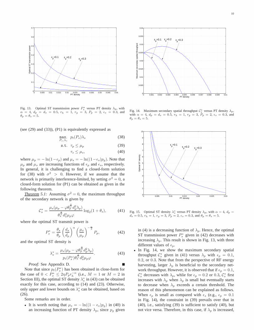
Fig. 13. Optimal ST transmission powerP ∗

s versus PT densityλp, withα = 4, dp = ds = 0.5, rh = 1, rg = 3, Pp = 2, ǫs = 0.3, andθp = θs = 5.

(see (29) and (33)), (P1) is equivalently expressed as

max.Ps,λs

pt(Ps)λs (38)

s.t. τp ≤ µp (39)

τs ≤ µs, (40)

whereµp = − ln(1−ǫp) andµs = − ln((1−ǫs)pg). Note thatµp andµs are increasing functions ofǫp andǫs, respectively.In general, it is challenging to find a closed-form solutionfor (38) with σ2 > 0. However, if we assume that thenetwork is primarily interference-limited, by settingσ2 = 0, aclosed-form solution for (P1) can be obtained as given in thefollowing theorem.

Theorem 5.1: Assumingσ2 = 0, the maximum throughputof the secondary network is given by

C∗

s =µs(µp − ϕθ

2αp d2pλp)

θ2αs d2sµpϕ

log2(1 + θs), (41)

where the optimal ST transmit power is

P ∗

s =θsθp

(

dsdp

)α(µs

µp

)−α2

Pp, (42)

and the optimal ST density is

λ∗

s =µs(µp − ϕθ

2αp d2pλp)

pt(P ∗s )θ

2αs d2sµpϕ

. (43)

Proof: See Appendix D.Note that sincept(P ∗

s ) has been obtained in close-form forthe case of0 < P ∗

s ≤ 2ηPpr−αh (i.e., M = 1 or M = 2 in

Section III), the optimal ST densityλ∗

s in (43) can be obtainedexactly for this case, according to (14) and (23). Otherwise,only upper and lower bounds onλ∗

s can be obtained, based on(26).

Some remarks are in order.• It is worth noting thatµs = − ln((1 − ǫs)pg) in (40) is

an increasing function of PT densityλp, sincepg given

0 0.001 0.002 0.003 0.004 0.005 0.006 0.007 0.008 0.009 0.010

0.005

0.01

0.015

0.02

0.025

0.03

0.035

0.04

PT density

Max

imum

sec

onda

ry s

patia

l thr

ough

put

εp=0.1 ε

p=0.2 ε

p=0.3

Fig. 14. Maximum secondary spatial throughputC∗

s versus PT densityλp,with α = 4, dp = ds = 0.5, rh = 1, rg = 3, Pp = 2, ǫs = 0.3, andθp = θs = 5.

0 0.005 0.01 0.015 0.02 0.025 0.030

1

2

3

4

5

6

7

8

9

10

PT density

Opt

imal

ST

den

sity

εp=0.1

εp=0.3ε

p=0.2

Fig. 15. Optimal ST densityλ∗

s versus PT densityλp, with α = 4, dp =ds = 0.5, rh = 1, rg = 3, Pp = 2, ǫs = 0.3, andθp = θs = 5.

in (4) is a decreasing function ofλp. Hence, the optimalST transmission powerP ∗

s given in (42) decreases withincreasingλp. This result is shown in Fig. 13, with threedifferent values ofǫp.

• In Fig. 14, we show the maximum secondary spatialthroughputC∗

s given in (41) versusλp with ǫp = 0.1,0.2, or 0.3. Note that from the perspective of RF energyharvesting, largerλp is beneficial to the secondary net-work throughput. However, it is observed that ifǫp = 0.1,C∗

s decreases withλp, whlie for ǫp = 0.2 or 0.3, C∗

s firstincreases withλp whenλp is small but eventually startsto decrease whenλp exceeds a certain threshold. Thereason of this phenomenon can be explained as follows.When ǫp is small as compared withǫs (e.g., ǫp = 0.1in Fig. 14), the constraint in (39) prevails over that in(40), i.e., satisfying (39) is sufficient to satisfy (40), butnot vice versa. Therefore, in this case, ifλp is increased,

11

the active STs’ densityptλs or C∗

s will be decreased toreduceτp in (39), i.e., reducing the network interferencelevel. However, whenǫp is relatively larger (e.g.,ǫp = 0.2or 0.3 in Fig. 14), (40) prevails over (39). As a result, ifλp is increased, then so isµs in (40), and thusptλs orC∗

s will be increased. However, ifλp exceeds a certainthreshold,ptλs will be decreased to reduceτs in (40); asa result,C∗

s decreases with increasingλp.• It is revealed from (43) that for givenλp, the optimal

active STs’ densitypt(P ∗

s )λ∗

s is fixed under a givenpair of primary and secondary outage constraints. Inother words,λ∗

s is inversely proportional topt(P ∗

s ). Thisimplies that aspt converges to zero withλp → 0 (seeFig. 7),λ∗

s diverges to infinity at the same time, as shownin Fig. 15. Thus, although the sparse PT density will leadto larger secondary network throughput (see Fig. 14), acorrespondingly large number of STs need to be deployedto achieve the maximum throughput, each with a verysmall transmission probabilitypt. As a result, only asmall fraction of the STs could be active at any time,resulting in large delay for secondary transmissions orinefficient secondary network design.

VI. A PPLICATION AND EXTENSION

In this section, we extend our results on the CR networkto the application scenario depicted in Fig. 2, where a set ofdistributed wireless power chargers (WPCs) are deployed topower wireless information transmitters (WITs) in a sensornetwork. It is assumed that wireless power transmission fromWPCs to WITs is over a dedicated band which is differentfrom that for the information transfer, and thus does notinterfere with wireless information receivers (WIRs). Forsimplicity, we assume that the path-loss exponents for boththepower transmission and information transmission are equaltoα. Moreover, the network models for WPCs and WITs as wellas the energy harvesting and transmission models of WITs aresimilarly assumed as in Section II for PTs and STs in the CRsetup. For convenience, we thus use the same symbol notationsfor PTs and STs to represent for WPCs and WITs, respectively.

A. Transmission Probability

Unlike the CR case, WITs in a sensor network do not needto be prevented from transmissions by guard zones, since thereare no PTs present. As a result, a WIT can transmit at anytime provided that it is fully charged. By lettingrg = 0,we havepg = 1, and from (14), (23) and (26) we obtainthe transmission probability of a typical WIT in the followingcorollary.

Corollary 6.1: The transmission probability of a typicalWIT is given by

1) If 0 < Ps ≤ ηPpr−αh or M = 1,

pt =ph

1 + ph. (44)

2) If ηPpr−αh < Ps ≤ 2ηPpr

−αh or M = 2,

pt =ph

ph + 1 + p2

ph

. (45)

0 0.01 0.02 0.03 0.04 0.05 0.06 0.07 0.080

0.05

0.1

0.15

0.2

0.25

WPC density

WIT

tran

smis

sion

pro

babi

lity

M=1 (Ps=0.1): Simulation

M=1 (Ps=0.1): Analysis

M=2 (Ps=0.2): Simulation

M=2 (Ps=0.2): Analysis

Fig. 16. WIT transmission probabilitypt versus WPC densityλp, withα = 4, η = 0.1, rh = 1, rg = 3, andPp = 1.

3) If Ps > 2ηPpr−αh or M > 2,

p1 + p′2

p1 + p′2 + 1 +p′

2

p1+p′

2

≤ pt ≤ph

ph + 1 +p′

2+p3

ph

, (46)

whereph = 1−e−πr2hλp is given in (9);p1 = 1−e−πh21λp and

p2 = e−πh21λp − e−πr2hλp are given in (19) and (21), respec-

tively; p′2 = e−πλph21 − e−πλph

22 andp3 = e−πλph

22 − e−πλpr

2h

are given in (24) and (25), respectively.It is worth noting that unlike the CR setup,pt in this case

is in general an increasing function ofλp since there are noguard zones and thus largerλp always help charge WITs morefrequently, as shown in Fig. 16.

B. Network Throughput Maximization

Note that unlike the CR setup, here we only need to considerthe outage probability of a typical WIR at the origin due to theinterference of other active WITs. Similar to Assumption 1,we assume that active WITs form an HPPP with densityptλs;thus, the outage probability of a typical WIR at the origin canbe obtained by simplifying Lemma 4.1 as

P(s)out

= Pr

{

gsPsd−αs

Is + σ2< θs

}

(47)

= 1− exp (−τs) , (48)

where in this caseτs is given by

τs = θ2αs d2sϕptλs +

θsdαs σ

2

Ps

. (49)

For the sensor network throughput maximization, Problem(P1) can be modified such that only the outage constraint forthe WIR is applied. Thus we have the following simplifiedproblem.

(P2) : max.Ps,λs

pt(Ps)λs log2(1 + θs) (50)

s.t. P(s)out

≤ ǫs. (51)

12

The solution of (P2) is given in the following corollary, basedon Theorem 5.1.

Corollary 6.2: Assumingσ2 = 0, the maximum networkthroughput is given by

C∗

s =µ′

s

θ2αs d2sϕ

log2(1 + θs), (52)

whereµ′

s = − ln(1− ǫs), and the optimal solution(P ∗

s , λ∗

s) ∈R+ × R+ is any pair satisfying

pt(P∗

s )λ∗

s =µ′

s

θ2αs d2sϕ

. (53)

Proof: With σ2 = 0, from (48) and (49), Problem (P2)can be equivalently rewritten as

maxPs,λs

pt(Ps)λs (54)

s.t. pt(Ps)λs ≤µ′

s

θ2αs d2sϕ

, (55)

whereµ′

s = − ln(1 − ǫs). To maximizept(Ps)λs, then it iseasy to see from (55) that the optimal solution ispt(P

∗

s )λ∗

s =µ′

s

θ2αs d2

sϕ

; by multiplying it with log2(1 + θs), we then obtain

C∗

s in (52).

Note that unlike the result in Theorem 5.1, the maximumnetwork throughput remains constant regardless ofλp. Thisis because there is no primary outage constraint in this caseand thus the optimal density of active WITspt(P ∗

s )λ∗

s isdetermined solely by the outage constraint of WIRs. On theother hand, ifλp is increased, we can effectively reduce therequired WIT densityλ∗

s for achieving the sameC∗

s sinceptin general increases withλp.

VII. C ONCLUSION

In this paper, we have proposed a novel network architectureenabling secondary users to harvest energy as well as reusethe spectrum of primary users in the CR network. Based onstochastic-geometry models and certain assumptions, our studyrevealed useful insights to optimally design the RF energypowered CR network. We derived the transmission probabilityof a secondary transmitter by considering the effects of boththe guard zones and harvesting zones, and thereby charac-terized the maximum secondary network throughput underthe given outage constrains for primary and secondary users,and the corresponding optimal secondary transmit power andtransmitter density in closed-form. Moreover, we showed thatour result can also be applied to the wireless sensor networkpowered by a distributed WPC network, or other similarwireless powered communication networks.

APPENDIX APROOF OFPROPOSITION3.3

For both the upper and lower bounds, similar to the caseof M = 2, we apply a 3-state Markov chain with state space{0, 1, 2} with states0, 1 and2 denoting the battery power levelof 0, in the range[ 12Ps, Ps), and equal toPs, respectively.

First, consider the upper bound onpt. Since the harvestedpower in the regiona(X,h2, rh) is assumed to be equal to12Ps, it is easy to see that the state transition-probability matrixfor this case is given by

P(u) =

1− ph p′2 + p3 p10 1− ph phpg 0 1− pg

. (56)

Let π(u) = [π(u)0 , π

(u)1 , π

(u)2 ] denote the steady-state probabil-

ity vector in this case. Solvingπ(u)P

(u) = π(u), we obtain

π(u)2 = ph

ph+pg

(

1+p′2+p3

ph

) and thus the upper bound onpt can

be obtained by multiplyingπ(u)2 with pg, according to (10).

Next, consider the lower bound onpt. Since the harvestedpower in the regiona(X,h2, rh) is assumed to be0, it is easyto obtain the state transition-probability matrix for thiscase as

P(l) =

1− (p1 + p′2) p′2 p10 1− (p1 + p′2) p1 + p′2pg 0 1− pg

. (57)

Similarly to the derivation of the upper bound onpt, thelower bound onpt can be found by finding the correspondingsteady-state probabilityπ(l)

2 =p1+p′

2

(p1+p′

2)+pg

(

1+p′2

p1+p′2

) , and

then multiplying it with pg. The proof of Proposition 3.3 isthus completed.

APPENDIX BPROOF OFLEMMA 4.1

For convenience, we derive the non-outage probability1−P

(p)out

as follows withP (p)out

given in (28).

1− P(p)out

= Pr

{

gpPpd−αp

Ip + Is + σ2≥ θp

}

(58)

= Pr

{

gp ≥θpd

αp

Pp

(

Ip + Is + σ2)

}

(59)

= EIp

[

EIs

[

exp

(

−θpd

αp

Pp

(

Ip + Is + σ2)

)]]

(60)

= exp

(

−θpd

αp

Pp

σ2

)

EIp

[

exp

(

−θpd

αp

Pp

Ip

)]

EIs

[

exp

(

−θpd

αp

Pp

Is

)]

, (61)

where in (61), the expectations are separated sinceIp andIsare assumed to be independent as a result of Assumption 1.Note that EIp

[

exp(

−θpd

αp

PpIp

)]

and EIs

[

exp(

−θpd

αp

PpIs

)]

are Laplace transforms in terms of the random variablesIp and

Is, respectively, both with input parameterθpd

αp

Pp. According

to the result in [26, 3.21], the Laplace transform of the shot-noise process of an HPPPΛ(λ) with densityλ > 0, denotedby I =

∑

T∈Λ(λ) gTP |T |−α, with input parameters is givenby

EI [exp(−sI)] = exp(−(Ps)2αλϕ), (62)

where {gT }T∈Λ(λ) is a set of i.i.d. exponential randomvariables with mean1, and ϕ is given in Lemma 4.1. Us-ing (62), we can easily obtainEIp

[

exp(

−θpd

αp

PpIp

)]

and

13

Admissible set

Optimal point

Ps

ptλs

ptλs = f1(Ps)

ptλs = f2(Ps)

Fig. 17. Illustration of the optimal solution for Problem (P1).

EIs

[

exp(

−θpd

αp

PpIs

)]

and by substituting them to (61), theproof of Lemma 4.1 is thus completed.

APPENDIX CPROOF OFLEMMA 4.2

The termPr{

gsPsd−αs

Ip+Is+σ2 < θs

}

in (32) is obtained by fol-lowing the similar procedure in the proof of Lemma 4.1, givenby

Pr

{

gsPsd−αs

Ip + Is + σ2< θs

}

= 1− exp(τs), (63)

whereτs is given in (34).Next, under the assumptionPp ≫ Ps, it is reasonable to as-

sume that the interference from even only one single PT insideb(Yo, rg) is sufficient to cause an outage to the typical SR at

the origin. Consequently, we havePr{

gsPsd−αs

Ip+Is+σ2 < θs∣

∣E}

≈

1. Substituting this result, (63) andPr{E} = e−πr2gλp = 1−pginto (32) yields (33). The proof of Lemma 4.2 is thus com-pleted.

APPENDIX DPROOF OFTHEOREM 5.1

From (30) and (34), the constraintsτp ≤ µp and τs ≤ µs

given in (39) and (40) are equivalent topt(Ps)λs ≤ f1(Ps)andpt(Ps)λs ≤ f2(Ps), respectively, where

f1(Ps) =

1

θ2αp d2pϕ

(

µp −θpd

αpσ

2

Pp

)

− λp

(

Ps

Pp

)−2α

,

(64)

f2(Ps) =1

θ2αs d2sϕ

(

µs −θsd

αs σ

2

Ps

)

− λp

(

Ps

Pp

)−2α

. (65)

As illustrated in Fig. 17,f1(Ps) decreases whereasf2(Ps)increases with growingPs. The shaded region in Fig. 17 showsthe admissible set of(Ps, ptλs) that satisfies the given outageprobability constraints. It is observed that the optimal valueof pt(Ps)λs is the intersection of the two curvespt(Ps)λs =f1(Ps) and pt(Ps)λs = f2(Ps). The intersection point can

be found by solvingf1(Ps) = f2(Ps), which has no closed-form solution in general withσ2 > 0. However, by lettingσ2 = 0, the closed-form solution ofP ∗

s can be obtained asθsθp

(

ds

dp

)α (µs

µp

)−α2

Pp. From pt(P∗

s )λ∗

s = f1(P∗

s ) and (64),

we then obtainpt(P ∗

s )λ∗

s =µs(µp−ϕθ

2αp d2

pλp)

θ2αs d2

sµpϕ

, and accordingly

λ∗

s =µs(µp−ϕθ

2αp d2

pλp)

pt(P∗

s )θ2αs d2

sµpϕ

. Theorem 5.1 is thus proved.

REFERENCES

[1] T. Le, K. Mayaram, and T. Fiez, “Efficient far-field radio frequency energyharvesting for passively powered sensor networks,”IEEE J. Solid-StateCircuits, vol. 43, no. 5, pp. 1287-1302, May 2008.

[2] A. M. Zungeru, L. M. Ang, S. Prabaharan, and K. P. Seng, “Radio fre-quency energy harvesting and management for wireless sensor networks,”Green Mobile Devices and Netw.: Energy Opt. Scav. Tech., CRC Press,pp. 341-368, 2012.

[3] R. J. M. Vullers, R. V. Schaijk, I. Doms, C. V. Hoof, and R. Mertens,“Micropower energy harvesting,”Elsevier Solid-State Circuits, vol. 53,no. 7, pp. 684-693, July 2009.

[4] D. Bouchouicha, F. Dupont, M. Latrach, and L. Ventura, “AmbientRF energy harvesting,”Int. Conf. Renew. Energies and Power Qual.(ICREPQ), Mar. 2010.

[5] T. Paing, J. Shon, R. Zane, and Z. Popovic, “Resistor emulation approachto low-power RF energy harvesting,”IEEE Trans. Power Elect., vol. 23,no. 3, pp. 1494-1501, May 2008.

[6] H. Jabbar, Y. S. Song, and T. T. Jeong, “RF energy harvesting system andcircuits for charging of mobile devices,”IEEE Trans. Consumer Elect.,vol. 56, no. 1, pp. 247-253, Feb. 2010.

[7] C. K. Ho and R. Zhang, “Optimal energy allocation for wireless commu-nications with energy harvesting constraints,”IEEE Trans. Sig. Process.,vol. 60, no. 9, pp. 4808-4818, Sep. 2012.

[8] O. Ozel, K. Tutuncouglu, J. Yang, S. Ulukus, and A. Yener,“Transmis-sion with energy harvesting nodes in fading wireless channels: optimalpolicies,” IEEE J. Sel. Areas Commun., vol. 29, no. 8, pp.1732-1743, Sep.2011.

[9] K. Huang, “Spatial throughput of mobile ad hoc networks with energyharvesting,”to appear in IEEE Trans. Inf. Theory (Available on-line athttp://arxiv.org/abs/1111.5799).

[10] D. Niyato, E. Hossain, and A. Fallahi, “Sleep and wakeupstrategies insolar-powered wireless sensor/mesh networks: performance analysis andoptimization,” IEEE Trans. Mobile Computing, vol. 6, no. 2, pp. 221-236,Feb. 2007.

[11] W. C. Brown, “The history of power transmission by radiowaves,”IEEETrans. Microwave Theory and Tech., vol. 32, pp. 1230-1242, Sep. 1984.

[12] L. R. Varshney, “Transporting information and energy simultaneously,”in Proc. IEEE Int. Symp. Inf. Theory (ISIT), pp. 1612-1616, July 2008.

[13] P. Grover and A. Sahai, “Shannon meets Tesla: wireless informationand power transfer,” inProc. IEEE Int. Symp. Inf. Theory (ISIT), pp.2363-2367, June 2010.

[14] R. Zhang and C. K. Ho, “MIMO broadcasting for simultaneous wirelessinformation and power transfer,”IEEE Trans. Wireless Commun., vol. 12,no. 5, pp. 1989-2001, May 2013.

[15] X. Zhou, R. Zhang, and C. K. Ho, “Wireless information and powertransfer: architecture design and rate-energy tradeoff,”submitted to IEEETrans. Commun. (Available on-line at http://arxiv.org/abs/1205.0618)

[16] L. Liu, R. Zhang, and K. C. Chua, “Wireless information transfer withopportunistic energy harvesting,”IEEE Trans. Wireless Commun., vol. 12,no. 1, pp. 288-300, Jan. 2013.

[17] K. Huang and V. K. N. Lau, “Enabling wireless power transfer incellular networks: architecture, modeling and deployment,” submitted forpublication. (Available on-line at http://arxiv.org/abs/1207.5640)

[18] S. Haykin, “Cognitive radio: brain-empowered wireless communica-tions,” IEEE J. Sel. Areas Commun., vol. 23, no. 2, pp. 201-220, Feb.2005.

[19] Q. Zhao and B. M. Sadler, “A survey of dynamic spectrum access,”IEEE Sig. Process. Mag., vol. 24, no. 3, pp. 79-89, May 2007.

[20] R. Zhang, Y. C. Liang, and S. Cui, “Dynamic resource allocation incognitive radio networks,”IEEE Sig. Process. Mag., vol. 27, no. 3, pp.102-114, May 2010.

14

[21] C. Yin, L. Gao, and S. Cui, “Scaling laws for overlaid wireless networks:a cognitive radio network versus a primary network,”IEEE/ACM Trans.Netw., vol. 18, no. 4, pp. 1317-1329, Aug. 2010.

[22] K. Huang, V. K. N. Lau, and Y. Chen, “Spectrum sharing betweencellular and mobile ad hoc networks: transmission-capacity trade-off,”IEEE J. Sel. Areas Commun., vol. 27, no. 7, pp. 1256-1267, Sep. 2009.

[23] J. Lee, J. G. Andrews, and D. Hong, “Spectrum sharing transmissioncapacity,” IEEE Trans. Wireless Commun., vol. 10, no. 9, pp. 3053-3063,Sep. 2011.

[24] C. H. Lee and M. Haenggi, “Interference and outage in Poisson cognitivenetworks,”IEEE Trans. Wireless Commun., vol. 11, no. 4, pp. 1392-1401,Apr. 2012.

[25] L. Xie, Y. Shi, Y. T. Hou, and H. D. Sherali, “Making sensor networksimmortal: an energy-renewal approach with wireless power transfer,”IEEE/ACM Trans. Netw., vol. 20, no. 6, pp. 1748-1761, Dec. 2012.

[26] M. Haenggi and R. K. Ganti, “Interference in large wireless networks,”Found. Trends in Netw., NOW Publishers, vol. 3, no. 2, pp. 127-248,2008.

[27] S. Weber and J. G. Andrews, “Transmission capacity of wirelessnetworks,” Found. Trends in Netw., NOW Publishers, vol. 5, no. 2-3,pp. 109-281, 2012.

[28] J. F. C. Kingman,Poisson processes. Oxford University Press, 1993.