operator splitting methods for non-autonomous differential...
TRANSCRIPT

OPERATOR SPLITTING METHODS FORNON-AUTONOMOUS DIFFERENTIAL
EQUATIONS
A Thesis Submitted tothe Graduate School of Engineering and Sciences of
Izmir Institute of Technologyin Partial Fulfillment of the Requirements for the Degree of
MASTER OF SCIENCE
in Mathematics
bySıla Ovgu KORKUT
December 2011IZMIR

We approve the thesis of Sıla Ovgu KORKUT
Assoc. Prof. Dr. Gamze TANOGLUSupervisor
Prof. Dr. Turgut OZISCommittee Member
Prof. Dr. Ali Ihsan NESLITURKCommittee Member
16 December 2011
Prof. Dr. Oguz YILMAZ Prof. Dr. Tugrul SengerHead of the Department of Dean of the Graduate School ofMathematics Engineering and Sciences

ACKNOWLEDGMENTS
I would like to express my sincere gratitude to my advisor Gamze TANOGLU for
her help, understanding, encouragement and patience during my studies.
I would like to thank to The Scientific and Technological Research Council of
Turkey (TUBITAK) for its financial support.
I owe the same amount of thanks to my family for being perpetually proud of me
without any reason.
It is my pleasure to thank Selin SOYSAL, Aslı ALTAS and Nurcan GUCUYENEN
for their helps.
Especially, I would like to thank foremost to Umut UYSAL for his positiveness to
me and for his endless supports .

ABSTRACT
OPERATOR SPLITTING METHODS FOR NON-AUTONOMOUS DIFFERENTIALEQUATIONS
In this thesis, convergency and stability analysis are studied for the non-autonomo-
us differential equations. Not only classical operator splitting methods; Lie Trother split-
ting, symmetrically weighted splitting and Strang splitting but also iterative splitting
method which is recent popular technique of operator splitting methods are considered.
We concentrate on how to improve the operator splitting methods with the help of the
Magnus expansion. In addition, we construct a new symmetric iterative splitting scheme.
Then, we also study its convergence properties by using the concepts of stability, con-
sistency and order. For this purpose, we use C0 semigroup techniques. Finally, several
numerical examples are illustrated in order to confirm our theoretical results by compar-
ing the new symmetric iterative splitting method with frequently used operator splitting
methods.
iv
OZET
ZAMANA BAGLI DENKLEMLER ICIN OPERATOR AYIRMA METODLARI
Bu tezde zamana baglı denklemler icin yakınsaklık ve kararlılık analizleri incelen-
mistir. Sadece klasik operator ayırma methodları; Lie Trother splitting, symmetrically
weighted splitting ve Strang splitting degil aynı zamanda operator ayırma metodlarının
son zamanlarda populer olan teknigi iterative splitting metodu da ele alınmıstır. Operator
ayırma metodlarını Magnus seri acılımı ile nasıl gelistirildigine yogunlasılmıstır. Buna
ek olarak, yeni bir simetrik iterative splitting seması olusturulmustur. Sonra bu metodun
kararlılık, tutarlılık ve mertebe konseptleri ile yakınsaklık ozellikleri uzerine calısılmıstır.
Bu amacla, C0 yarıgrup teknikleri kullanılmıstır. Son olarak, teorik sonucları dogrulamak
icin yeni simetrik iterative splitting methodu ile sık kullanılan operator ayırma methodları
karsılastırılarak numerik ornekler gosterilmistir.
v

TABLE OF CONTENTS
LIST OF FIGURES . . . . . . . . . . . . . . . . . . . . . . . . . . . . . . . . . . . . . . . . . . . . . . . . . . . . . . . . . . . . . . . . . . . . . . . viii
LIST OF TABLES . . . . . . . . . . . . . . . . . . . . . . . . . . . . . . . . . . . . . . . . . . . . . . . . . . . . . . . . . . . . . . . . . . . . . . . . ix
CHAPTER 1. INTRODUCTION . . . . . . . . . . . . . . . . . . . . . . . . . . . . . . . . . . . . . . . . . . . . . . . . . . . . . . . 1
1.1. Introduction . . . . . . . . . . . . . . . . . . . . . . . . . . . . . . . . . . . . . . . . . . . . . . . . . . . . . . . . . . . . 1
1.2. Layout of the Thesis . . . . . . . . . . . . . . . . . . . . . . . . . . . . . . . . . . . . . . . . . . . . . . . . . . . 3
CHAPTER 2. MAGNUS EXPANSION . . . . . . . . . . . . . . . . . . . . . . . . . . . . . . . . . . . . . . . . . . . . . . . 5
2.1. Magnus Expansion . . . . . . . . . . . . . . . . . . . . . . . . . . . . . . . . . . . . . . . . . . . . . . . . . . . . 5
2.2. Convergency of Magnus Expansion . . . . . . . . . . . . . . . . . . . . . . . . . . . . . . . . . . 7
CHAPTER 3. OPERATOR SPLITTING METHODS BASED ON MAGNUS
EXPANSION . . . . . . . . . . . . . . . . . . . . . . . . . . . . . . . . . . . . . . . . . . . . . . . . . . . . . . . . . . . . 9
3.1. Lie-Trotter Splitting Based on Magnus Expansion . . . . . . . . . . . . . . . . . . 9
3.2. Symmetrically Weighted Splitting Based on Magnus Expansion . . . 10
3.3. Strang Splitting Based on Magnus Expansion . . . . . . . . . . . . . . . . . . . . . . . 11
3.4. Iterative Splitting Method . . . . . . . . . . . . . . . . . . . . . . . . . . . . . . . . . . . . . . . . . . . . . 12
3.4.1. Algorithm for Iterative Splitting . . . . . . . . . . . . . . . . . . . . . . . . . . . . . . . . . . 12
3.5. New Symmetric Iterative Splitting Method . . . . . . . . . . . . . . . . . . . . . . . . . . 16
CHAPTER 4. CONSISTENCY ANALYSIS OF OPERATOR SPLITTING
METHODS . . . . . . . . . . . . . . . . . . . . . . . . . . . . . . . . . . . . . . . . . . . . . . . . . . . . . . . . . . . . . . 19
4.1. Consistency Analysis for Bounded Operators . . . . . . . . . . . . . . . . . . . . . . . 19
4.1.1. Error Analysis of Lie Trotter Splitting . . . . . . . . . . . . . . . . . . . . . . . . . . . 19
4.1.2. Error Analysis of Strang Splitting . . . . . . . . . . . . . . . . . . . . . . . . . . . . . . . . 20
4.1.3. Error Analysis of Symmetrically Weighted Splitting . . . . . . . . . . . 22
4.1.4. Error Analysis of Iterative Splitting . . . . . . . . . . . . . . . . . . . . . . . . . . . . . 24
4.2. Consistency Analysis for Unbounded Operators . . . . . . . . . . . . . . . . . . . . 25
4.2.1. Semigroup Theory . . . . . . . . . . . . . . . . . . . . . . . . . . . . . . . . . . . . . . . . . . . . . . . . 26
4.2.2. Assumptions . . . . . . . . . . . . . . . . . . . . . . . . . . . . . . . . . . . . . . . . . . . . . . . . . . . . . . . 28
4.2.3. Analysis . . . . . . . . . . . . . . . . . . . . . . . . . . . . . . . . . . . . . . . . . . . . . . . . . . . . . . . . . . . . 29
vi

4.2.3.1. Lie-Trotter Splitting . . . . . . . . . . . . . . . . . . . . . . . . . . . . . . . . . . . . . . . . 29
4.2.3.2. Strang Splitting . . . . . . . . . . . . . . . . . . . . . . . . . . . . . . . . . . . . . . . . . . . . . 30
4.2.3.3. Symmetrically Weighted Splitting . . . . . . . . . . . . . . . . . . . . . . . . 32
4.2.4. Symmetric Iterative Splitting . . . . . . . . . . . . . . . . . . . . . . . . . . . . . . . . . . . . 34
CHAPTER 5. STABILITY ANALYSIS FOR OPERATOR SPLITTING
METHODS . . . . . . . . . . . . . . . . . . . . . . . . . . . . . . . . . . . . . . . . . . . . . . . . . . . . . . . . . . . . . . 37
5.1. Stability for Autonomous Linear ODE Systems . . . . . . . . . . . . . . . . . . . . . 37
5.1.1. Stability Analysis for Bounded Operators . . . . . . . . . . . . . . . . . . . . . . . 37
5.1.2. Stability Analysis for Unbounded Operators . . . . . . . . . . . . . . . . . . . . 39
5.2. Stability for Non-autonomous Linear ODE Systems . . . . . . . . . . . . . . . . 42
5.2.1. Stability Analysis of Sequential Splitting . . . . . . . . . . . . . . . . . . . . . . . . 43
5.2.2. Stability Analysis of Strang-Marchuk Splitting . . . . . . . . . . . . . . . . . 44
5.2.3. Stability Analysis of Symmetrically Weighted Splitting . . . . . . . . 44
5.2.4. Stability Analysis of Symmetric Iterative Splitting . . . . . . . . . . . . . . 46
CHAPTER 6. CONVERGENCY ANALYSIS FOR OPERATOR SPLITTING
METHODS . . . . . . . . . . . . . . . . . . . . . . . . . . . . . . . . . . . . . . . . . . . . . . . . . . . . . . . . . . . . . . 48
6.1. Convergence analysis of the Traditional Methods . . . . . . . . . . . . . . . . . . . 48
6.2. Convergency of Proposed Method . . . . . . . . . . . . . . . . . . . . . . . . . . . . . . . . . . . . 49
CHAPTER 7. NUMERICAL EXPERIMENTS . . . . . . . . . . . . . . . . . . . . . . . . . . . . . . . . . . . . . . . 51
7.1. Mathieu equation . . . . . . . . . . . . . . . . . . . . . . . . . . . . . . . . . . . . . . . . . . . . . . . . . . . . . . 51
7.2. Radial Schrodinger equation . . . . . . . . . . . . . . . . . . . . . . . . . . . . . . . . . . . . . . . . . 54
7.3. Schrodinger Equation . . . . . . . . . . . . . . . . . . . . . . . . . . . . . . . . . . . . . . . . . . . . . . . . 57
CHAPTER 8. CONCLUSION . . . . . . . . . . . . . . . . . . . . . . . . . . . . . . . . . . . . . . . . . . . . . . . . . . . . . . . . . . 60
REFERENCES . . . . . . . . . . . . . . . . . . . . . . . . . . . . . . . . . . . . . . . . . . . . . . . . . . . . . . . . . . . . . . . . . . . . . . . . . . . 61
APPENDIX A. MAT-LAB CODES . . . . . . . . . . . . . . . . . . . . . . . . . . . . . . . . . . . . . . . . . . . . . . . . . . . . . 65
vii

LIST OF FIGURES
Figure Page
Figure 7.1. Comparison of 2nd order Magnus and first order approximation for
equation (7.1) for various schemes for small time step h = 0.01 on
[0, 10]. . . . . . . . . . . . . . . . . . . . . . . . . . . . . . . . . . . . . . . . . . . . . . . . . . . . . . . . . . . . . . . . . . . . . . . . . 53
Figure 7.2. Comparison of 2nd order Magnus and first order approximation for
equation (7.1) for various schemes for small time step h = 0.01 on
[0, 10]. . . . . . . . . . . . . . . . . . . . . . . . . . . . . . . . . . . . . . . . . . . . . . . . . . . . . . . . . . . . . . . . . . . . . . . . . 53
Figure 7.3. Comparison first order methods for equation (7.4) for small time step
h = 0.0001 on [0, 6]. . . . . . . . . . . . . . . . . . . . . . . . . . . . . . . . . . . . . . . . . . . . . . . . . . . . . . . . . . 55
Figure 7.4. Comparison of exact and approximation solution for equation (7.4) for
various schemes for small time step h = 0.0001 on [0, 6]. . . . . . . . . . . . . . . . . 56
Figure 7.5. Comparison fourth order Magnus expansion and second order SISM for
equation (7.4) for small time step h = 0.0001 on [0, 6]. . . . . . . . . . . . . . . . . . . . 57
Figure 7.6. The probability of density, |Ψ(x, t)|2, for the particle in (7.12) with
ω2(t) = 4− 3e−t by using the symmetric iterative splitting. . . . . . . . . . . . . . . 58
Figure 7.7. The probability of density, |Ψ(x, t)|2, for the particle in (7.12) with
ω2(t) = cos2(t) by using SISM2. . . . . . . . . . . . . . . . . . . . . . . . . . . . . . . . . . . . . . . . . . . 59
viii
LIST OF TABLES
Table Page
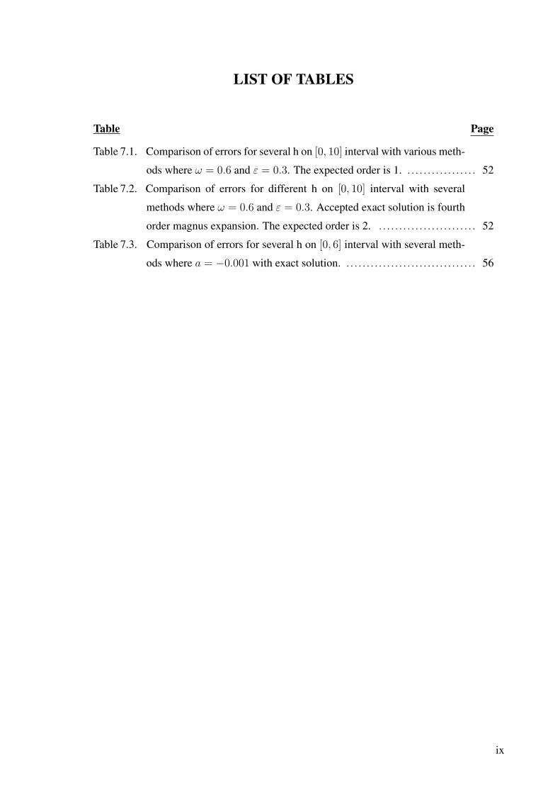
Table 7.1. Comparison of errors for several h on [0, 10] interval with various meth-
ods where ω = 0.6 and ε = 0.3. The expected order is 1. . . . . . . . . . . . . . . . . . 52
Table 7.2. Comparison of errors for different h on [0, 10] interval with several
methods where ω = 0.6 and ε = 0.3. Accepted exact solution is fourth
order magnus expansion. The expected order is 2. . . . . . . . . . . . . . . . . . . . . . . . . 52
Table 7.3. Comparison of errors for several h on [0, 6] interval with several meth-
ods where a = −0.001 with exact solution. . . . . . . . . . . . . . . . . . . . . . . . . . . . . . . . . 56
ix

CHAPTER 1
INTRODUCTION
1.1. Introduction
Operator splitting is a widely used procedure in the numerical solution of large
systems of partial differential equations. It can be regarded as a time-discretization method.
Thus, it can be called as time splitting method. The basic idea behind the operator splitting
methods is based on splitting of complex problem into simpler sub-problems. Then, each
of which are solved by an efficient method. The connections between the sub-systems are
the initial conditions. Instead of the original problem, we deal with simpler sub-problem.
Thus, this technique gives rise to error which is called splitting error. This error can be
estimated theoretically.
The idea of sequential splitting, which is known as Lie-Trotter splitting, dates back
to the 1950s. In (Bagrinovskii and Gudunov, 1957), this method was first applied to a
partial differential equations. During the years 1960-1970, the first splitting methods were
developed. They were in connection with finite difference methods. A renovation of the
methods was done in the 1980s while using the methods for complex processes underlying
partial differential methods (Crandall and Majda, 1980). The simplest kind is sequential
splitting, which, in terms of the local splitting error, is the first order accurate in time.
A second order and, therefore, more popular method is Strang splitting in (Marchuk,
1968), (Strang, 1968). In (Strang, 1963), Strang proposed a splitting method where a
weighted sum of splitting solutions, obtained by different ordering of the sub-operators,
are computed at each time step. The symmetrically weighted sequential (SWS) splitting is
second order accurate, as popular as Strang splitting. Its analysis can be found by Csomos
et al. in (Csomos et al., 2003). There is another sort of splitting method, iterative splitting,
which is recently popular technique of operator splitting methods. The earliest detection
of iterative method era 1995s, (Kelly, 1995), was seemingly far in advance of its time.
In (Kanney et al., 2003), they focused on the convergence of iterative splitting procedure
for nonlinear reactive transport problems. In (Farago and Geiser, 2007), they suggest a
new scheme which is based on the combination of splitting time interval and traditional
iterative operator splitting. Then, this technique is used in (Geiser, 2008); (Geiser, 2008).
In the current study, we propose a new method which is found by the combining with the
1

Magnus expansion and the iterative operator splitting which is suggested in (Farago and
Geiser, 2007).
Magnus integrators are an interesting class of numerical methods for Hamiltonian
problems. The problem which Magnus expansion (ME) solves has a history dating back
at least to the study of Peano, by the end of 19th century, and Baker at the beginning of
the 20th. They combine the theory of differential equations with an algebraic formula-
tion. In connection with these treatments from the beginning, is the study of so called
Baker-Campbell-Hausdorff formula. (Magnus, 1954) have been considered as birth cer-
tificate of Magnus Expansion. The work of Pechukas and Light gave for the first time
a more specific convergence analysis of the problem than the ambiguous considerations
in Magnus paper. Wei and Norman did the same for existence problem. The study of
Robinson, (Robinson, 1963), seems to be the first application of the ME to a physical
problem. During the years between 1971 and 1990, ME was successfully applied to a
wide spectrum of fields in Physics and Chemistry. In the last decay of 20th century ME
has been adapted for specific types of equations: Floquet theory, stochastic differential
equations etc. In numerical analysis, using ME as a geometric integrator along the lines
of work pioneered by Iserles and Nørsett in (Iserles and Nørsett, 1999).
In this thesis, to discuss the analysis and applications, we concentrate on an ap-
proximate solution of non-autonomous systems of the following form
d
dtu(t) = A(t)u(t), t ≥ 0
u(0) = u0 ∈ X
on some (complex) Banach space X with the norm ∥.∥X←X . Since the Magnus expansion
(Blanes et al., 2008); (Blanes and Moan, 2006) is an attractive and widely applied method
of solving explicitly time-dependent problems, in order to solve such non-autonomous
system, as a numerical method, we apply operator splitting methods combining with Mag-
nus expansion. It is often the case that A(t) = T+V (t), where only the potential operator
V (t) is time-dependent and T is the differential operator see (Baye et al., 2003); (Baye
et al., 2004); (Chin and Chen, 2002); (Aguilera-Navarro et al., 1990); (Chin and Anisi-
mov, 2006). To analyze the convergence of the given methods, we study on two different
approaches;
• For the case of T and V (t) are bounded, we use Taylor series expansion.
• For the case of T is unbounded and V (t) is bounded, we use C0 semigroup ap-
2

proaches
The idea of using strongly continuous semigroup (C0 semigroup) approaches for
the convergency of operator splitting methods as an abstract homogeneous Cauchy prob-
lem goes back at least to Pazy in (Pazy, 1983). Bjørhus analyze the operator splitting
method for the linear inhomogeneous abstract Cauchy problem in (Bjørhus, 1998). In
the paper (Batkai et al., 2011), they investigate the convergence of operator splitting
methods by using evolution semigroups. You can also see (Jahnke and Lubich, 2000);
(Hansen and Ostermann, 2009) for obtaining estimates on the order of convergence. By
this to investigate the convergence of any method, the concepts of stability, consistency
and order are used. Both (Geiser and Tanoglu, 2011) and (Geiser, 2008) deal with the
consistency of different splitting schemes has been thoroughly investigated in the terms of
the local splitting error for autonomous systems. In addition, the convergence of iterative
splitting method for the autonomous case in (Gucuyenen and Tanoglu, 2011). In this
thesis, we focused on the convergence of introduced splitting methods and especially the
convergence of the new iterative splitting method.
1.2. Layout of the Thesis
Our aim is to develop and analyze the operator splitting methods combining with
Magnus expansion. In particular, we focused on iterative splitting method. The main
object of this thesis will be two fold: First, we construct a new symmetric iterative split-
ting scheme for non-autonomous problem. Second, its convergence properties are ana-
lyzed using the concepts of stability, consistency, and order as an abstract Cauchy problem
via analytic semigroup approach. Finally, we test these schemes on several numerical ex-
amples to confirm our theoretical results.
The purpose of Chapter 2 is to present Magnus expansion for solving the time-
dependent part of problem. We also give some conditions for convergence of Magnus
expansion (ME). The next step in present thesis is to combine Magnus expansion with
operator splitting methods. Thus, Chapter 3 introduces the operator splitting methods,
which are based on Magnus expansions. In the first, we give the algorithm of traditional
operator splitting methods. Then we embedded ME into operator splitting methods. We
concentrate on to construct a new algorithm for the iterative splitting method which has
time-symmetry property.
In Chapter 4, the consistency of the methods are discussed. Not only bounded
3

case but also unbounded case is considered. Chapter 5 deals with in detail the stability
issue for general case of the splitting methods, which are introduced in previously. We
study this issue as an abstract Cauchy problem. In Chapter 6, we present the convergence
results of the splitting methods which follow the line of telescoping identity and ”Lady
windermere’s fan” argument.
In Chapter 7, we give some numerical examples to confirm our theoretical re-
sults and to demonstrate the effectiveness of suggested scheme. For this purpose, we use
ODEs and PDEs. Since ME is an attractive and widely applied method of solving explic-
itly harmonic oscillator, we test our method in Matheui equation. We compare our new
scheme with traditional schemes in this test problem. Since its efficiency, we apply it into
Schrodinger equation. We present the results as tables and figures.
Finally, we conclude with a brief discussion of the study fulfilled in Chapter 8.
4

CHAPTER 2
MAGNUS EXPANSION
In the present chapter, we summarize a brief overview of Magnus expansion (ME).
In order to present our point of view of ME, we may distinguish two main directions :
• We report the recurrence formulation of Magnus expansion.
• For what values of t does the series converge ? We describe this question as the
convergence problem. Thus, in Section 2.2 we will sum up the convergence condi-
tions for the ME.
2.1. Magnus Expansion
The Magnus integrator was introduced as a tool to solve non-autonomous linear
differential equations for linear operators of the form
du
dt= A(t)u(t) , (2.1)
with solution
u(t) = exp(Ω(t))u(0). (2.2)
This can be expressed as:
u(t) = T(exp(
∫ t
0
A(s) ds
)u(0) , (2.3)
where the time-ordering operator T is given in (Dyson, 2008).
5

The Magnus expansion is defined as:
Ω(t) =∞∑n=1
Ωn(t) , (2.4)
where the first few terms are (Blanes et al., 2008):
Ω1(t) =
∫ t
0
dt1A1
Ω2(t) =1
2
∫ t
0
dt1
∫ t1
0
dt2[A1, A2]
Ω3(t) =1
6
∫ t
0
dt1
∫ t1
0
dt2
∫ t2
0
dt3([A1, [A2, A3] + [A3, [A1, A2]])
· · · · · · etc. (2.5)
where An = A(tn). In practice, it is more useful to define the nth order Magnus operator
Ω[n](t) = Ω(t) +O(tn+1) (2.6)
such that
u(t) = exp[Ω[n](t)
]u(0) +O(tn+1). (2.7)
Thus, the second-order Magnus operator is
Ω[1](t) =
∫ t
0
dt1A(t1)
= etA(12t) +O(t3) (2.8)
or
Ω[1](t) =
∫ t
0
dt1A(t1)
= et(A(t))+(A(0))
2 +O(t3). (2.9)
6

and a fourth-order Magnus operator (Blanes et al., 2008); (Blanes and Moan, 2006) is
Ω[4](t) =1
2t(A1 + A2)− c3t
2[A1, A2] (2.10)
where A1 = A(c1t), A2 = A(c2t) and
c1 =1
2−
√3
6, c2 =
1
2+
√3
6, c3 =
√3
12. (2.11)
The necessity of doing time integrations and evaluating nested commutators make Mag-
nus integrators beyond the fourth-order rather complex.
Remark 2.1 The Magnus expansion can be generalized in different ways, e.g., commuta-
torless expansion, Volsamber iterative method, Floquet-Magnus expansion, etc. (Blanes
et al., 2008). However, none reduces the number of needed operators at high orders.
2.2. Convergency of Magnus Expansion
To study the convergence of the Magnus expansion, we investigate the conditions
on A(t). In the pioneering work Wilhelm Magnus studied its convergence in 1954. He
proposed the Magnus series does not converge unless t is sufficiently small value. In
literature, many bounds to the actual radius of convergence in terms of A(t) have been
obtained. For achieving this radius, the following statement is used.
Proposition 2.1 If Ωm(t) denotes the homogeneous element with m− 1 commutators in
the Magnus series, then Ω(t) =∑∞
m=1 is absolutely convergent for 0 ≤ t < T ,
T = max
t ≥ 0 :
∫ t
0
∥A(s)∥2ds < rc
. (2.12)
Both Pechukas and Light (Pechukas and Light, 2008) and Karasev and Mosolova
(Karasev and Mosolova, 1977) obtained rc = ln 2 = 0.6931.... In 1987, Strichartz
(Strichartz, 1987) had rediscovered the explicit expression for Ωn found by Bialynicki-
Birula et al. (Bialynicki-Birula et al., 1969), stated in terms of Lie brackets. He used this
7

to prove rc = 1. This bound is improved independently in 1998 by Blanes et al. (Blanes
et al., 1998) and Moan (Moan, 1998) as rc = 1.086868.... In 2001, Moan and Oteo
(Moan and Oteo, 2001) derived the bound rc = 2 by similar techniques, except that they
avoided the use of commutators as they seemed to introduce needless complications in
the convergence bound. Finally, Moan and Niesen have been able to prove that rc = π if
only real matrices are involved.
8
CHAPTER 3
OPERATOR SPLITTING METHODS BASED ON MAGNUS
EXPANSION
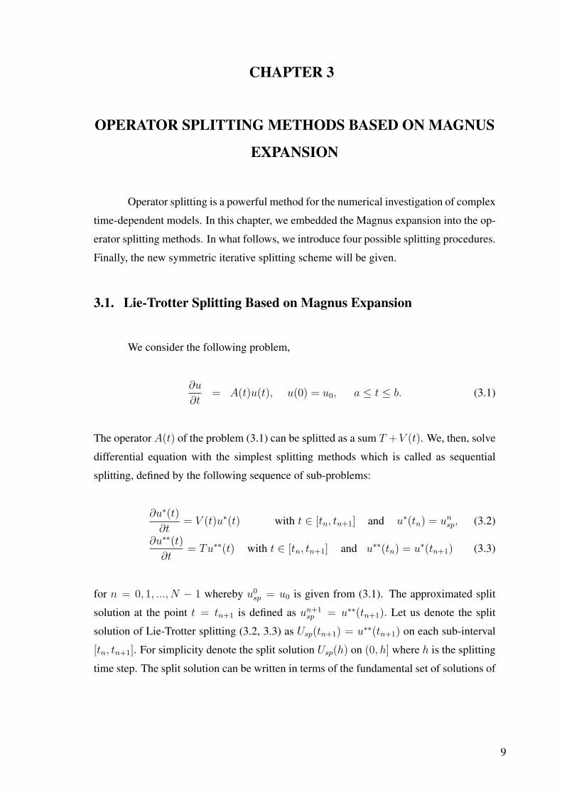
Operator splitting is a powerful method for the numerical investigation of complex
time-dependent models. In this chapter, we embedded the Magnus expansion into the op-
erator splitting methods. In what follows, we introduce four possible splitting procedures.
Finally, the new symmetric iterative splitting scheme will be given.
3.1. Lie-Trotter Splitting Based on Magnus Expansion
We consider the following problem,
∂u
∂t= A(t)u(t), u(0) = u0, a ≤ t ≤ b. (3.1)
The operator A(t) of the problem (3.1) can be splitted as a sum T +V (t). We, then, solve
differential equation with the simplest splitting methods which is called as sequential
splitting, defined by the following sequence of sub-problems:
∂u∗(t)
∂t= V (t)u∗(t) with t ∈ [tn, tn+1] and u∗(tn) = un
sp, (3.2)
∂u∗∗(t)
∂t= Tu∗∗(t) with t ∈ [tn, tn+1] and u∗∗(tn) = u∗(tn+1) (3.3)
for n = 0, 1, ..., N − 1 whereby u0sp = u0 is given from (3.1). The approximated split
solution at the point t = tn+1 is defined as un+1sp = u∗∗(tn+1). Let us denote the split
solution of Lie-Trotter splitting (3.2, 3.3) as Usp(tn+1) = u∗∗(tn+1) on each sub-interval
[tn, tn+1]. For simplicity denote the split solution Usp(h) on (0, h] where h is the splitting
time step. The split solution can be written in terms of the fundamental set of solutions of
9

each sub equations (3.2, 3.3) as
Usp(h) = eTh eΩV (h)u0 (3.4)
where the exponent ΩV (h) is an infinite sum of nested integrals and commutators belongs
to the time dependent operator V (t) explained in Section (2.1). To analyze the order of the
Lie-Trotter splitting, we need to compare (3.4) with the exact solution of unsplit problem
which we will write in the form
u(h) = eΩA(h)u0 (3.5)
where the exponent ΩA(h) is an infinite sum of nested integrals and commutators belong
to the time dependent operator A(t) explained in Section (2.1). If we rearranged the
equation (3.5) by substituting the ΩA(h) then, we have
u(h) = ehA(h/2)u0. (3.6)
3.2. Symmetrically Weighted Splitting Based on Magnus Expansion
We consider A(t) = T + V (t). The weighted splitting can be obtained by using
two sequential splittings as in the following algorithm:
∂u∗(t)
∂t= V (t)u∗(t) with t ∈ [tn, tn+1] and u∗(tn) = un
sp, (3.7)
∂u∗∗(t)
∂t= Tu∗∗(t) with t ∈ [tn, tn+1] and u∗∗(tn) = u∗(tn+1) (3.8)
and
∂v∗(t)
∂t= Tv∗(t) with t ∈ [tn, tn+1] and v∗(tn) = vnsp, (3.9)
∂v∗∗(t)
∂t= V (t)v∗∗(t) with t ∈ [tn, tn+1] and v∗∗(tn) = v∗(tn+1) (3.10)
10
for n = 0, 1, ..., N − 1 whereby u0sp = u0 is given from (3.1). The approximated split
solution at the point t = tn+1 is defined as un+1sp = u∗∗(tn+1). Let us denote the split
solution of Lie-Trotter splitting (3.2, 3.3) as Usp(tn+1) = u∗∗(tn+1) on each sub-interval
[tn, tn+1]. The split solution can be written in terms of the fundamental set of solutions of
each sub equations (3.9, 3.10) as
U∗sp(h) = eΩV (h) eThu0. (3.11)
The numerical solution is computed as a weighted average of the solutions obtained by the
two sequential splitting steps. Let us denote the split solution of symmetrically weighted
splitting(SWS) as Usw(tn+1) on sub-interval. Therefore, we can write the split solution as
follows,
Usw(h) =Usp(h) + U∗sp(h)
2
Usw(h) =eTh eΩV (h) + eΩV (h) eTh
2u0. (3.12)
3.3. Strang Splitting Based on Magnus Expansion
We split the A(t) as in previous techniques. Then, we apply another splitting
technique which is known as Strang-Marchuk splitting, where for one splitting time-step
three sub-problems should be solved:
∂u∗(t)
∂t= Tu∗(t), with t ∈ [tn, tn+1/2] and u∗(tn) = un
sp (3.13)
∂u∗∗(t)
∂t= V (t)u∗(t), with t ∈ [tn, tn+1] and u∗∗(tn) = u∗(tn+1/2), (3.14)
∂u(t)
∂t= T u(t), with t ∈ [tn+1/2, tn+1] and u(tn+1/2) = u∗∗(tn+1) (3.15)
for n = 0, 1, ..., N − 1 whereby u0sp = u0 is given from (3.1). The approximated split
solution at the point t = tn+1 is defined as un+1sp = u∗∗(tn+1). Let us denote the split
solution of Strang Marchuk splitting (3.2, 3.3) as Usm(tn+1) = u(tn+1) on each sub-
interval [tn, tn+1]. For simplicity denote the split solution Usm(h) on (0, h] where h is the
11

splitting time step. The split solution can be written in terms of the fundamental set of
solutions of each sub equations (3.13, 3.15) as
Usm(h) = eTh/2 eΩV (h) eTh/2u0. (3.16)
Example 3.1 By substituting the ΩV (h) as in equation (2.8) which is given in section
(2.1), we get
eΩ[2](h) = eh[T+V (h/2)]
= e12hT ehV (h/2)e
12hT +O(h3). (3.17)
3.4. Iterative Splitting Method
In the present section, we will introduce traditional iterative splitting method. In
this thesis our main focus is to create a new scheme for iterative splitting method. In the
subsection 3.5, we develop the proposed method.
3.4.1. Algorithm for Iterative Splitting
In this section, we summarize brief overview the iterative splitting scheme. We
consider the following problem,
∂u
∂t= (A+B)u(t), u(0) = u0. (3.18)
where A and B are linear operators and u0 is initial condition.
The method is based on iteration by fixing the splitting discretization step size
h on time interval [tn, tn+1]. The following algorithms are then solved consecutively for
i = 1, 3, . . . , 2p+ 1.∂ui
∂t= Aui(t) +Bui−1(t) with ui(tn) = un, (3.19)
∂ui+1
∂t= Aui(t) +Bui+1(t) with ui+1(tn) = un (3.20)
12

where un is the known split approximation at time level t = tn and u0 ≡ 0 is our initial
guess. The split approximation at the time-level t = tn+1 is defined as un+1 = u2p+2(tn),
see (Geiser, 2009); (Farago and Geiser, 2007).
The exact solutions of this system of equation then can be written by using the
variation of constant formula as follows:
ui(t) = exp(At)u0 +
∫ t
0
exp((t− s)A)Bui−1(s) ds (3.21)
ui+1(t) = exp(Bt)u0 +
∫ t
0
exp((t− s)B)Aui(s) ds. (3.22)
We summarize our algorithm in the following steps:
• Step 1: Consider the time interval [t0, tend], divide it into N subintervals so that
time step is h = (tend − t0)/N .
• Step 2: On each subinterval, [tn, tn + h], n = 0, 1..N , use the algorithm by consid-
ering the initial conditions for each step as u(t0) = u0, ui(tn) = ui−1(tn) = u(tn),
ui(tn + h) = eA(tn+h)u0 + A−1Bui−1(tn+1)− A−1ehABui−1(tn)
ui+1(tn + h) = eB(tn+h)u0 +B−1Aui(tn+1)−B−1ehBAui(tn)
where tn+1 denotes tn + h.
• Step 3: Check the condition
|ui − ui−1| ≤ Tol,
if it is satisfied stop the iteration on this interval,
• Step 4: ui(tn + h) → u(tn + h)
• Step 5: Repeat this procedure for the next interval until the desired time T is
achieved.
Theorem 3.1 Let A, B ∈ L(X), where X is a Banach space, be given linear bounded
operators. The Cauchy problem is in (3.18). Then the problem has a unique solution. The
error bounds of the iterations (3.19), (3.20) are given by
13

• for i is odd
∥ei∥ ≤ (K1.∥A∥)i−12 .(K2.∥B∥)
i+12 .∥e0∥
ti
i!, (3.23)
• for i is even
∥ei∥ ≤ (K1.∥A∥)i2 .(K2.∥B∥)
i2 .∥e0∥
ti
i!(3.24)
where ∥e0∥ is the difference between the exact solution and initial guess,
∥exp(At)∥ ≤ K1, ∥exp(Bt)∥ ≤ K2 for t ≥ 0.
Proof The algorithms of the method are given by
u′i(t) = Aui(t) +Bui−1(t) (3.25)
u′i+1(t) = Aui(t) +Bui+1(t) (3.26)
with initial condition ui(0) = u0 and ui+1(0) = u0 where i = 1, 3, . . . , 2p+ 1 for [0, t].
For the first iteration, from the variation of constant formula, we have
=⇒ u1(t) = eAtu0 +
∫ t
0
eA(t−s)Bu0 ds, (3.27)
and we know the exact solution
=⇒ u(t) = eAtu0 +
∫ t
0
eA(t−s)Be(A+B)su0 ds. (3.28)
For the second iteration, from the variation of constant formula, we have
=⇒ u2(t) = eBtu0 +
∫ t
0
eB(t−s)Au1 ds (3.29)
14

and we know the exact solution
=⇒ u(t) = eBtu0 +
∫ t
0
eB(t−s)Ae(A+B)su0 ds. (3.30)
Let’s denote ei = u(t) − ui(t). Assume that A, B are linear bounded operators and
∥exp(At)∥ ≤ K1, ∥exp(Bt)∥ ≤ K2 for t ≥ 0.
For i = 1, we have the error bound
∥u(t)− u1(t)∥ = ∥∫ t
0
eA(t−s)B(e(A+B)su0 − u0) ds∥ (3.31)
∥e1∥ = ∥∫ t
0
eA(t−s)Be0 ds∥ (3.32)
∥e1∥ ≤ K1.∥B∥.∥e0∥t, (3.33)
for i = 2, we get
∥u(t)− u2(t)∥ = ∥∫ t
0
eB(t−s)A(e(A+B)su0 − u1) ds∥ (3.34)
∥e2∥ = ∥∫ t
0
eB(t−s)A(e1) ds∥ (3.35)
∥e2∥ ≤ K2
∫ t
0
∥A∥.∥e1∥ ds (3.36)
∥e2∥ ≤ K2.K1.∥A∥.∥B∥.∥e0∥t2
2(3.37)
and for i = 3
∥u(t)− u3(t)∥ = ∥∫ t
0
eA(t−s)B(e(A+B)su0 − u2) ds∥ (3.38)
∥e3∥ = ∥∫ t
0
eA(t−s)Be2 ds∥ (3.39)
∥e3∥ ≤ K1
∫ t
0
∥B∥.∥e2∥ ds (3.40)
∥e3∥ ≤ K1.K2.K1.∥B∥.∥A∥.∥B∥.∥e0∥t3
6(3.41)
then by induction we get:
15
For i is odd
∥ei∥ ≤ (K1.∥A∥)i−12 .(K2.∥B∥)
i+12 .∥e0∥
ti
i!(3.42)
For i is even
∥ei∥ ≤ (K1.∥A∥)i2 .(K2.∥B∥)
i2 .∥e0∥
ti
i!. (3.43)
Note that in (Farago et al., 2008) they give the same error bounds implicitly. This explicit
form can be found in (Gucuyenen and Tanoglu, 2011).
Remark 3.1 Iterative splitting method provides the higher order accuracy in approxi-
mate solution with increasing number of iteration steps.
3.5. New Symmetric Iterative Splitting Method
Let us consider the initial value problem (IVP ) given in (3.1) on the time interval
[0, tend] where tend ∈ R. We assume for A(t) a two-term splitting
T + V (t).
Let us divide the integration interval [0, tend] in N equal parts by the points t0, t1, ...., tn,
where the length of each interval is h = tn+1 − tn = tend/N, j = 0, 1..N − 1. The
approximated solution and exact solution at time t = tn are U(tn) and u(tn), respectively.
Our technique is close to that used in (Blanes and Ponsoda, 2008). We apply
second order iterative process described as below on each subinterval [tn, tn+1],
u1 = Tu1 + V (t)U(t0) u1(tn) = U(tn) (3.44)
u2 = Tu1 + V (t)u2 u2(tn) = U(tn) (3.45)
where u2(tn) = U(tn) denotes the numerical approximation to the true solution u(tn) at
16

the time t = tn and U(t0) = u0. The formal solution of the sub equations given in (3.44)
and (3.45) on the time interval [t, t+ h] can be written by
ui(t+ h) = Φi(t+ h, t)ui(t) +
∫ t+h
t
Φi (t+ h, s)Fi(s) ds, i = 1, 2
where F1 = V (t)U(t) and F2 = Tu1(t+ h). Furthermore, Φi is given as follows
Φ1(t+ h, t) = e(h)T
Φ2(t+ h, t) = eh2[V (t+h)+V (t)]
which is the second order approximation of the Magnus series given in equation (2.9).
Next we use the trapezoidal rule to approximate the integral
∫ t+h
t
Φi Fi ds =h
2[Fi(t+ h) + Φi(t+ h, t)Fi(t)] +O(h3). (3.46)
Note that Φi(t + h, t + h) = I. After combining approximation (3.46) with the iterative
schemes (3.44), (3.45) and rearranging expressions, we get the first order approximation
u1(tn + h) = eTh[u1(tn) +h
2V (tn)u0(tn)] +
h
2V (tn + h)u0(tn) (3.47)
and the second order approximation,
u2(tn + h) = eh2[V (tn+h)+V (tn)][U(tn) +
h
2Tu1(tn)] +
h
2Tu1(tn + h) (3.48)
where Un+1 = u2(tn + h). Repeat this procedure for next interval until the desired time
tend is reached.
Proposition 3.1 New iterative scheme preserve the time-symmetry property.
Proof
The time- symmetry preservation can be easily seen by interchanging tn+1,
17

ui(tn+1), h by tn, ui(tn), −h, respectively.
un1 = e−hT [un+1
1 − h
2V (tn+1)u
n0 ]−
h
2V (tn)u
n0 . (3.49)
By rearranging the equation (3.49), we have
ehT [un1 +
h
2V (tn)u
n0 ] = [un+1
1 − h
2V (tn+1)u
n0 ]
un+11 = ehT [un
1 +h
2V (tn)u
n0 ] +
h
2V (tn+1)u
n0 .
Similarly, when we consider the second order scheme to prove the time symmetry prop-
erty, we use the same procedure as above.
un2 = e−
h2[V (tn)+V (tn+1)][un+1
2 − h
2Tun+1
1 ]− h
2Tun
1 . (3.50)
When we arrange the equation (3.50) for un+12 , they are equivalent to equations in (3.45).
18

CHAPTER 4
CONSISTENCY ANALYSIS OF OPERATOR SPLITTING
METHODS
In chapter (3), we obtained modified first and second order splitting methods with
the help of the Magnus expansion. This chapter is related to find the error bound for these
methods. We will study on the following equation
d
dtu(t) = A(t)u(t) = (T + V (t))u(t), 0 ≤ t ≤ tend (4.1)
u(0) = u0 ∈ X.
where X is any Banach space and A(t) = T + V (t).
4.1. Consistency Analysis for Bounded Operators
The main idea of this section is to analyze the error bounds for the bounded oper-
ators, T and V (t). These bounds are represented with the help of Taylor expansion in the
following subsections.
4.1.1. Error Analysis of Lie Trotter Splitting
Proposition 4.1 The Lie-Trotter splitting is at least first order for the system of equation
given as (4.1) with the error bound
∥u(h)− Usp(h)∥ ≤ A1h2. (4.2)
Here A1 only depends on ∥[T, V (h/2)]∥ and ∥u0∥.
19

Proof The numerical split solution (3.4) takes the following form after using the Taylor
expansion for eTh and the second order Magnus expansion as in (2.8) for eΩV (h)
Usp(h) = (I + Th+1
2T 2h2 +O(h3))(I + V (
h
2)h+
1
2V 2(
h
2)h2 +O(h3))u0.(4.3)
After collecting the terms under the powers of h, we have
Usp(h) = (I + (T + V (h
2))h+ (
1
2V 2(
h
2) + TV (
h
2) +
1
2T 2)h2 +O(h3))u0.(4.4)
We will approximate the exact solution (3.5) up to the second order also according
to Magnus expansion which is proposed in (2.8). This yields
u(h) = (I + (T + V (h
2))h+
1
2(V 2(
h
2) + TV (
h
2) + V (
h
2)T + T 2)h2
+ O(h3))u0 (4.5)
where A(t) = T + V (t). In order to find the error bound, we compare (4.4) with the
exact solution (4.5). Subtracting (4.4) from (4.5) leads to
u(h)− Usp(h) =1
2(TV (
h
2)− V (
h
2)T )h2 u0 +O(h3). (4.6)
Hence, the error bound of Lie-Trotter splitting is
∥u(h)− Usp(h)∥ ≤ 1
2∥[T, V (h/2)]∥∥u0∥h2. (4.7)
20

4.1.2. Error Analysis of Strang Splitting
Proposition 4.2 The Strang-Marchuk splitting is at least second order for the system of
equation given as (4.1) with the error bound
∥u(h)− Usm(h)∥ ≤ A2h3
where A2 is a function of ∥T∥, ∥u0∥ and ∥V(t)∥.
Proof The numerical split solution which is defined in equation (3.16) as Strang split-
ting takes the following form after using the Taylor expansion for eTh and the second
order Magnus expansion which is given in equation (2.8) for eΩV (h)
Usm(h) = (I +1
2Th+
1
8T 2h2 +
1
48T 3h3 +O(h4))(I + V (
h
2)h+
1
2V 2(
h
2)h2
+1
6V 3(
h
2)h3 +O(h4))(I +
1
2Th+
1
8T 2h2 +
1
48T 3h3 +O(h4))u0.
After collecting the terms under the powers of h, we have
Usm(h) =
[I + (T + V (
h
2))h+ (
1
2V 2(
h
2) +
T
2V (
h
2) + V (
h
2)T
2+
1
2T 2)h2
+
(1
6V 3(
h
2) +
T 2V (h2) + V (h
2)T 2
8+
TV 2(h2)V 2(h
2)T
4
+TV (h
2)T
4+
1
6T 3
)h3
]u0 +O(h4). (4.8)
We will approximate the exact solution by using Magnus expansion as in numerical solu-
tion. This yields
u(h) =
[I + (T + V (
h
2))h+
1
2(V 2(
h
2) + TV (
h
2) + V (
h
2)T + T 2)h2
+1
6
(V 3(
h
2) + T 2V (
h
2) + TV (
h
2)T + TV 2(
h
2) + V (
h
2)T 2
+ V (h
2)TV (
h
2) + V 2(
h
2)T + T 3
)h3]u0 +O(h4) (4.9)
where A(t) = T + V (t).
21

Substraction the (4.9) and (4.8) leads to
u(h)− Usm(h) = [1
24(T 2V (
h
2) + V (
h
2)T 2)
− 1
12(TV 2(
h
2) + V 2(
h
2)T + TV (
h
2)T ) +
1
6V (
h
2)TV (
h
2)]h3u0
+ O(h4). (4.10)
The error bound of Strang splitting is obtained as
∥u(h)− Usm(h)∥ ≤ 1
12∥T 2V (
h
2)∥+ 1
6∥TV 2(
h
2)∥
+1
12∥TV (
h
2)T∥+ 1
6∥V (
h
2)TV (
h
2)∥∥u0∥h3. (4.11)
4.1.3. Error Analysis of Symmetrically Weighted Splitting
Proposition 4.3 The Symmetrically weighted splitting is at least second order for the
system of equation given as (4.1) with the error bound
∥u(h)− Usw(h)∥ ≤ A3h3. (4.12)
where A3 depends on ∥[T, [V (h2), T ]]∥ and ∥[V(h
2), [V(h
2),T]]∥ and ∥u0∥.
Proof
The symmetrically weighted splitting solution in (3.9, 3.10) takes the form
U∗sp(h) = (I + V (h
2)h+
1
2V 2(
h
2)h2 +
1
6V 3(
h
2)h3 +O(h4))(I + Th
+1
2T 2h2 +
1
6T 3h3 +O(h4))u0.
(4.13)
22

After collecting the terms under the powers of h, we have
U∗sp(h) =[I + (T + V (
h
2))h+ (
1
2V 2(
h
2) + TV (
h
2) +
1
2T 2)h2
+
(1
6V 3(
h
2) +
1
2V 2(
h
2)T
+1
2V (
h
2)T 2 +
1
6T 3
)h3 +O(h4)
]u0. (4.14)
and the symmetrically weighted solution is
Usw(h) =Usp(h) + U∗sp(h)
2u0,
or equal to
Usw(h) =
[I + (T + V (
h
2))h+
1
2(V 2(
h
2) + TV (
h
2) + V (
h
2)T + T 2)h2
+
(1
6V 3(
h
2) +
1
4TV 2(
h
2) +
1
4T 2V (
h
2) +
1
4V (
h
2)T 2
+1
4V 2(
h
2)T +
1
6T 3
)h3)u0 +O(h4). (4.15)
We know the exact solution is
u(h) =
[I + (T + V (
h
2))h+
1
2(V 2(
h
2) + TV (
h
2) + V (
h
2)T + T 2)h2
+1
6
(V 3(
h
2) + T 2V (
h
2) + TV (
h
2)T + TV 2(
h
2) + V (
h
2)T 2
+ V (h
2)TV (
h
2) + V 2(
h
2)T + T 3
)h3]u0 +O(h4) (4.16)
Subtracting (4.15) from (4.16) leads to
u(h)− Usw(h) =1
12([T, [V (
h
2), T ]] + [V (
h
2), [V (
h
2), T ]])u0h
3 +O(h4). (4.17)
Therefore, symmetrically weighted splitting is bounded by
∥u(h)− Usw(h)∥ ≤ 1
12(∥[T, [V (
h
2), T ]]∥+ ∥[V (
h
2), [V (
h
2), T ]]∥)∥u0∥h3. (4.18)
23

4.1.4. Error Analysis of Iterative Splitting
The operator A(t) of the problem (4.1) can be splitted as a sum T + V (t). We,
then, solve the following algorithms consecutively for i = 1, 3, . . . , 2p+ 1.
∂ui(t)
∂t= Tui(t) + V (t)ui−1(t) t ∈ [tn, tn+1] and ui(tn) = un
sp, (4.19)
∂ui+1(t)
∂t= Tui(t) + V (t)ui+1(t) t ∈ [tn, tn+1] and ui+1(tn) = un
sp (4.20)
for n = 0, 1, ..., N − 1 whereby u0sp = u0 is given from (4.1) and u0 ≡ 0 is our initial
guess. The split approximation at the time-level t = tn+1 is defined as Un+1itsp = ui+1(tn),
see (Geiser, 2009); (Farago and Geiser, 2007).
Proposition 4.4 The iterative splitting is at first order if we consider one iteration for the
system of equation given as (4.1) with the error bound
∥u(h)− Uitsp(h)∥ ≤ A4h2. (4.21)
Here A4 depends on ∥T∥ and ∥V (t)∥.
Proof
Each sub equation, (4.19) and (4.20) have the following solutions
u1(h) = eThu0 +
∫ h
0
eT (h−s)V (s)u0 for each [0, h], (4.22)
If we use the Taylor expansion for eTh, then (4.22) yields
u1(h) = (I + Th+1
2T 2h2)(I +
∫ h
0
(I − Ts)V (s)ds)u0.
24
Due to midpoint rule for approximating integral in (4.23), one obtains
u1(h) = (I + Th+1
2T 2h2)(
I + h(V (h
2)− h
2TV (
h
2)))u0 +O(h3). (4.23)
By rearranging the equation above, we have
u1(h) = (I + (V (h
2) + T )h+
1
2h2(T 2 + 2TV (
h
2) + V 2(
h
2)))u0
+ O(h3) (4.24)
where Uitsp(h) = u1(h). The exact solution is
u(h) = (I + (T + V (h
2))h+
1
2(V 2(
h
2) + TV (
h
2) + V (
h
2)T + T 2)h2)u0
+ O(h3). (4.25)
The error of the iterative splitting method is obtained by subtracting (4.24) from (4.25).
One obtains
∥u(h)− Uitsp(h)∥ ≤ 1
2(∥[T, V (
h
2)]∥∥u0∥h2. (4.26)
Proposition 4.5 The iterative splitting is at first order if we consider two iterations for
the system of equation given as (4.1) with the error bound
∥u(h)− Uitsp(h)∥ ≤ A5h3 (4.27)
where A5 depends on ∥T∥ and ∥V (t)∥.
Proof The proof follows the line of previous one.
25

4.2. Consistency Analysis for Unbounded Operators
In this section, our main aim is to illustrate the error bounds for operators which
are assumed T is unbounded and V (t) is bounded in Eq.(4.1). To obtain these bounds, we
commence with describing semigroup theory and employed assumptions. Then, we will
give error bounds the given methods.
4.2.1. Semigroup Theory
In the current subsection, we will summarize semigroup theory, since it will be
used to get some basic assumptions in the next subsection. This theory is developed to
solve operator ODE. Consider the initial value problem,
∂u(t)
∂t= Au(t) with t ∈ [0, tend], u(0) = u0, (4.28)
with given matrix A ∈ Rn×n. The solution of equation above can be written as following,
u(t) = etAu0. (4.29)
In preceding section, we represented if A is a linear bounded operator in Banach space,
U(t) still has this form. However, in many interesting cases, it is unbounded which don’t
admit this form. This to some extend shows the richness of semigroup theory.
For its application, semigroup theory uses abstract methods of operator theory to
treat initial boundary value problems for linear and nonlinear equations that describe the
evolution of a system.
Theorem 4.1 (Gelfand) Denote σ(M) = λ ∈ C|λI − M is not invertible to be the
spectrum of bounded linear operator A. We have
• σ(A) is closed bounded nonempty set in C
• Let | σ(M) |= maxλ∈σ(M) | λ |. We have σ(M) = limk→∞ | Mk | 1k .
Remark 4.1 For any power series, f(z) =∑
anzn, suppose the convergence circle of
f is B(0, R). Then if R >| σ(M) |, f(M) =∑
anMn is well-defined. For instance,
26

eM =∑
Mn
n!is well defined for any bounded operator M.
Definition 4.1 A one-parameter strongly continuous semigroup of operators over a real
or complex Banach space X is a map such that,
S : X 7→ X
i S(0)=I
ii for all t, s ≥ 0 S(t+ s) = S(t)S(s)
iii ∀x ∈ X such that ∥S(t)x− x∥ → 0 as t → 0.
The first two axioms are algebraic, and state that S(t) is a representation of the semigroup
(X,X); the last is topological, and states that the map S(t) is continuous in the strong
operator topology.
Theorem 4.2 S(t) be one-parameter semigroup of operator that is strongly continuous
at t = 0 then, there exist constants b, k such that S(t) ≤ bekt.
Definition 4.2 The infinitesimal generator A of S(t) is given by:
Ax := limt↓0
1
t(S(t)x− x)
whenever the limit exists and D(A) is its domain.
Theorem 4.3 S(t) be a strongly continuous semigroup of operators. Then,
• It is uniquely determined by its infinitesimal generator.
• if x ∈ D(A) then S(t)x ∈ D(A) and AS(t)x = S(t)Ax.
• D(An) is dense for any n ∈ N, where D(An) := u ∈ D(An−1)|An−1u ∈ D(A).
• A is closed operator.
For bounded linear operator M, the resolvent set is the complement of spectrum
σ(M), denote by ρ(M). So for any λ ∈ ρ(M), λI −M is invertible. And its resolvent is
R(λ) = (λI −M)−1. However for unbounded operator A, we need change the definition
to λI−A is bijective between D(A) and X . The resolvent of A is still R(λ) = (λI−A)−1,
27
but the map is X 7→ D(A). For any λ ∈ C whose real part is bigger than k( where
| S(t) |≤ bekt), we can define Laplace transform of S(t) by L(λ)x =∫∞0
e−λtS(t)xdt.
The following theorem states the properties of the resolvent of A.
Theorem 4.4 (Hille-Yosida) The infinitesimal generator A of contractions,i.e. | S(t) |≤1 for all t ≥ 0 has every positive, real in its resolvent and | R(λ) |=| (λI − A)−1 |≤ 1
λ.
The detailed proof of this theorem can be found in (Pazy, 1983).
4.2.2. Assumptions
For our analysis we need the following assumptions:
Assumption 4.1 Suppose that closed linear operator A(t) : D → X where D is dense
subset of X and that A(t) is uniformly sectorial for 0 ≤ t ≤ tend. Then, there exist
constants a ∈ R, 0 < φ < π/2,and M1 ≥ 1 such that Sφ(a) = λ ∈ C : | arg(a− λ) |≤φ ∪ a,
∥(λI − A(t))−1∥X←X ≤ M1
| (a− λ) |for any λ ∈ C \ Sφ(a). (4.30)
Then for fixed 0 ≤ s ≤ tend, the analytic semigroup etA(s)satisfy ∥ etA(s) ∥≤ Meωt for
some constants ω < 0 and M ≥ 1. Our general references on semigroups are (Oster-
mann et al., 2006), (Batkai et al., 2011).
Assumption 4.2 Let D(T ) = D(A(t)). We assume that T is linear closed operator and
that generates a strongly continuous semigroup etT on X. By semi group property, we
assume ∥ eTt ∥≤ 1.
Assumption 4.3 We assume that V (t) is bounded linear operator on X. Then we get
eΩV (t) ≤ et∥V (t)∥ where ΩV (t) ≈ Ω2(t) with the help of the equation (2.9). As the con-
vergence of Magnus expansion is guaranteed if ∥ Ω(t) ∥< π. The details can be found in
(Moan and Niesen, 2008).
Lemma 4.1 Let T be an infinitesimal generator of a C0 semigroup S(t), t ≥ 0. Let
tend > 0. If for any V (t)U ∈ D(T ) satisfying V (t)U, TV (t)U ∈ C1([0, tend];X) then the
28

solution of problem satisfies u(t) ∈ D(A2(t)) for 0 ≤ t ≤ tend whenever u0 ∈ D(A2(t)),
and we have
sup0≤t≤tend
∥T iu(t)∥ ≤ Ei(tend), i = 0, 1, 2 (4.31)
where Ei depends on the specific choice of tend, T, V (t)U and u0. For the detailed proof
see (Bjørhus, 1998).
Assumption 4.4 We assume that there are non-negative constants C, R with
sup0≤t≤tend
∥V (t)∥ ≤ C.
∥u∥ ≤ R on 0 ≤ t ≤ tend.
4.2.3. Analysis
Under the assumptions which are given in previous subsection, we will analyze
the consistency. In order to get the error bounds we use the techniques are close to that
use in (Jahnke and Lubich, 2000); (Hansen et al., 2008).
4.2.3.1. Lie-Trotter Splitting
Proposition 4.6 Let Assumption 4.2 and 4.4 be fulfilled. Then, the Lie Trotter splitting
method is first order accuracy, i.e., the local error satisfies the bound
∥u(h)− U(h)∥ ≤ C1h2 (4.32)
where C1 is a function of C and R.
Proof We start from the variation of constant formula for the exact solution
u(h) = eThu0 +
∫ h
0
eT (h)V (h− s)u(h− s)ds.
29

By using midpoint rule for approximating integral, we get
u(h) = eThu0 + heT (h)V (h/2)u(h/2) +O(h2).
Taylor expansion of u(0 + h/2) at t = 0 leads to
u(h) = eThu0 + heT (h)V (h/2)u(0) +O(h2). (4.33)
On the one hand, the split solution is given by
U(h) = eThu0 + heThV (h/2)u0 + F1. (4.34)
where
F1 =h2
2eThV 2(h/2)u0 +O(h3).
Due to our assumptions F1 is bounded by h2
2C2, i.e. F1 ≤ h2
2C2.
The proof follows the subtracting numerical solution in equation (4.34) from the
exact solution given in (4.33). Henceforth, we have
∥u(h)− U(h)∥ ≤ F1 +O(h2)
∥u(h)− U(h)∥ ≤ C1h2 (4.35)
where C1 is function of C and R.
4.2.3.2. Strang Splitting
We, now, show that Strang splitting method is consistent for the abstract Cauchy
problem in 4.1 under the assumptions which we determined in the subsection 4.2.2.
30

Proposition 4.7 Let Assumption 4.2 and 4.4 be fulfilled. Then, the Strang-Marchuk split-
ting is second order accuracy, i.e., the local error satisfies the bound
∥u(h)− U(h)∥ ≤ C2h3
where C2 is a function of C3, R.
Proof
We start with the numerical solution. Using Taylor expansion with the help of the
equation (2.8) for eΩV (h) leads
U(h) = eTh2 (I + hV (h/2) +
h2
2V 2(h/2) +
h3
6V 3(h/2) +O(h4))eT
h2 u0
= eThu0 + heTh2V (h/2)eT
h2 u0 +
h2
2eT
h2V 2(h/2)eT
h2 u0 + F2 (4.36)
where F2 =h3
6eT
h2V 3(h/2)eT
h2 u0 +O(h4). The bound of F2 follows the line of Assump-
tion 4.2 and 4.4 and it is defined as
F2 ≤h3
6C3 ∥u0∥.
On the other side, as in proof of proposition 4.6, we represent the variation of
constant formula for the exact solution. Expressing the last term of integral, we substitute
the u(h) by the same formula, at the end of this process we have
u(h) = eThu0 +
∫ h
0
eT (h−s)V (s)eTsu0 ds
+
∫ h
0
∫ s
0
eT (h−s)V (s)eT (s−ρ)V (ρ)eTρu(ρ)dρ ds. (4.37)
31

We define g1(s) = eT (h−s)V (s)eTsu0 and g2(s, ρ) = eT (h−s)V (s)eT (s−ρ)V (ρ)eTρu(ρ).
With the aid of g1(s), g2(s, ρ) the equation (4.37) can be rewritten as
u(h) = eThu0 +
∫ h
0
g1(s)u0 ds
+
∫ h
0
∫ s
0
g2(s, ρ)dρ ds. (4.38)
We use midpoint rule to approximate the integrals. Hence we obtain
u(h) = eThu0 + h(eTh2V (h/2)eT
h2 +O(h2))
+h2
2eT
h2V (h/2)V (h/2)eT
h2 u(h/2) +O(h3).
Again using Taylor expansion of u(0 + h/2) at t = 0 leads to
u(h) = eThu0 + h(eTh2V (h/2)eT
h2 ) +
h2
2eT
h2V 2(h/2)eT
h2 u0
+ O(h3). (4.39)
By subtracting (4.36) from (4.39), one obtains
∥u(h)− U(h)∥ ≤ ∥F1∥+O(h3)
∥u(h)− U(h)∥ ≤ C2h3 (4.40)
where C2 depends on eTh, V (h/2) and R. Therefore, by means of our assumptions,
C2 is bounded by a function of C3 and R.
32

4.2.3.3. Symmetrically Weighted Splitting
Proposition 4.8 Let Assumption 4.2 and 4.4 be fulfilled. Then, the symmetrically weighted
splitting is second order accuracy, i.e., the local error satisfies the bound
∥u(h)− U(h)∥ ≤ C3h3.
Proof
The proof proceeds by starting numerical solution. As in proof proposition 4.7,
using exponential series with the help of the equation (2.8) for eΩV (h) leads to
U(h) =eTh(I + hV (h/2) + h2
2V 2(h/2)) + (I + hV (h/2) + h2
2V 2(h/2))eTh
2u0
+ O(h3)
= eThu0 +h
2(eThV (h/2) + V (h/2)eTh)u0 +
h2
4(eThV 2(h/2) + V 2(h/2)eTh)u0
+ O(h3). (4.41)
Consequently, by variation of constants formula ,we obtain the following repre-
sentation of exact solution:
u(h) = eThu0 +
∫ h
0
eT (h−s)V (s)eTsu0 ds
+
∫ h
0
∫ s
0
eT (h−s)V (s)eT (s−ρ)V (ρ)eTρu0dρ ds+ F2
where
F3 =
∫ h
0
eT (h−s)V (s)
∫ s
0
eT (s−ρ)V (ρ)
∫ ρ
0
eT (ρ− ξ)V (ξ)u(ξ)dξ dρ ds
which is bounded by ∥F3∥ ≤ h3
6C3 ∥R∥. We define g(s) = eT (h−s)V (s)eTsu0 and ω(s, ρ) =
eT (h−s)V (s)eT (s−ρ)V (ρ)eTρu0. By using trapezium rule to approximate the integrals, i.e.
we substitute h2(g(h) + g(0)) for the second term and substitute h2
4(ω(0, 0) + ω(h, h)) for
33

the last term, one obtains
u(h) = eThu0 +h
2(V (h)eTh + eThV (0))u0 +
h2
4(eThV 2(0) + V 2(h)eTh)u0 +O(h3).
We use Taylor expansion of V (h/2 + h/2) at h/2 and also V (h/2− h/2) at h/2 leads to
u(h) = eThu0 +h
2(V (h/2)eTh + eThV (h/2))u0
+h2
4(eThV 2(h/2) + V 2(h/2)eTh)u0 +O(h3). (4.42)
In order to get the order of this method, we take a look at the error ej = ∥u(tj)− U(tj)∥.
Subtracting 4.41 from and using the assumptions leads to
∥u(h)− U(h)∥ ≤ C3h3. (4.43)
Here C3 is a function of C and R.
4.2.4. Symmetric Iterative Splitting
Proposition 4.9 The symmetric iterative splitting is first order if we consider only one
iteration given in (3.44) with the error bound
∥u(h)− U(h)∥ ≤ Kh2 (4.44)
Here K only depends on C, R,E1(tend).
Proof
We define the local error by ej = U(tj)− u(tj), j = 0, 1, 2, . . . , n. For simplicity,
we only consider the time interval [0,h]. The exact solution of the equation (4.1) can be
written as,
u(h) = eThu0 +
∫ h
0
eThV (h− s)u(h− s)ds. (4.45)
34

We derive the error bound for the equation (4.1) by using first order iterative splitting
scheme.Thus, the numerical solution of (4.1),
U(h) = eThu0 +
∫ h
0
eThV (h− s)u0ds. (4.46)
By subtracting (4.46) from (4.45) leads to
∥u(h)− U(h)∥ = ∥∫ h
0
eThV (h− s)[u(h− s)− u0]ds∥
≤ hC∥u(h− s)− u0∥ (4.47)
where C = sup0≤t≤tend∥V (t)∥. To obtain the error bound for ∥u(h) − u0∥ we use the
Lemma 4.1 and Assumption 4.4 ,
u(h) = u0 +
∫ h
0
A(s)u(s)ds
∥u(h)− u0∥ = h∥A(s)u∥ = h∥(T + V (s))u∥ ≤ h ∥ Tu ∥ + ∥ V (s)u ∥
∥u(h)− u0∥ ≤ h(E1(tend) + CR). (4.48)
By substituting (4.48) in the equation (4.47), we have
∥u(h)− U(h)∥ ≤ h2C(E1(tend) + CR) = Kh2 (4.49)
where K = C(E1(tend) + CR).
Proposition 4.10 The symmetric iterative splitting is the second order if we consider two
iterations given in (3.45) with the error bound
∥u(h)− U(h)∥ ≤ Kh3 (4.50)
Here K only depends on C, R,E1(tend).
35

Proof
We write the equation for second order iterative splitting as follows,
U(h) = eThu0 +
∫ h
0
eThV (h− s)u1ds. (4.51)
For estimating the error bound, we subtract the (4.51) from the equation (4.45), remaining
term is
∥u(h)− U(h)∥ = ∥∫ h
0
eThV (h− s)[u(h− s)− u1]ds∥
≤ hC∥u(h− s)− u1∥. (4.52)
Here u1 is the solution of the equation in (3.44). The proof follows that of the bound of
∥u(t− s)− u1∥ in (4.49), we have
∥u(h)− U(h)∥ ≤ h3C2(E1(tend) + CR) = h3K. (4.53)
36

CHAPTER 5
STABILITY ANALYSIS FOR OPERATOR SPLITTING
METHODS
This chapter deals with the stability of any linear ordinary differential equation
(ODE). We investigate this subject in two main fold. Firstly, the autonomous case is
considered both bounded and unbounded operators. In the sequel, non-autonomous case
is discussed.
5.1. Stability for Autonomous Linear ODE Systems
In this section, we summarize the stability issue in order not to ruin the general
flow of thesis. Our main reference on stability of linear autonomous differential equations
is the book Hundsdorfer and Verwer, see (Hundsdorfer and Verwer, 2003). To analyze
the stability of autonomous differential equations, we focused on the equation in (4.28)
with the exact solution (4.29).
5.1.1. Stability Analysis for Bounded Operators
In the present subsection, we take a look at properties of ODEs and particularly at
influence of perturbations at such systems. Consider the (IVP) in 4.28 with exact solution
. Then, take into account perturbed system,
∂U(t)
∂t= AU(t) + g(t) with t ∈ [0, tend], U(0) = U0. (5.1)
Then by subtracting equation (4.29) from the solution of equation (5.1) which is found by
using variation of constant formula, leads to
δ(t) = etAδ(0) +
∫ t
0
e(t−s)Aδ(s)ds (5.2)
37

where δ(t) denotes to U(t)− U(t). Then, the norm estimation can be found as
∥δ(t)∥ ≤ ∥etA∥∥δ(0)∥+∫ t
0
∥e(t−s)A∥ds max0≤s≤t
∥δ(s)∥.
As a result, if we have the following stability condition,
∥etA∥ ≤ Ketw for all t ≥ 0,
with constants K > 0 and w ∈ R. Therefore, we obtain
∥δ(t)∥ ≤ Ketw∥δ(0)∥+ K
t(etw − 1) max
0≤s≤t∥δ(s)∥, (5.3)
with arranging (etw − 1)/w = t in case w = 0. This inequality shows that the overall
error ∥δ(t)∥ can be bounded in terms of error ∥δ(0)∥ and perturbations ∥δ(s)∥, 0 ≤ s ≤ t.
In general, the term stability will be used to indicate that small perturbations give a small
overall effect. Next, we concentrate on bound for ∥etA∥. Suppose that A is diagonalizable,
that is A = PΛP−1, where Λ = diag(λk). Hence, the norm as follows,
∥etA∥ ≤ ∥P∥∥Λ∥∥P−1∥ = cond(P ) max1≤k≤t
| etλk | . (5.4)
Consequently, if we know that cond(P ) = ∥P∥∥P−1∥ ≤ K and Re(λk) ≤ w, then (5.3)
follows with
w = max1≤≤k≤m≤
| etλk | . (5.5)
In particular, if A is a normal matrix, i.e. A∗A = AA∗ where A∗ denotes conjugate
transpose of A, then the eigenvectors of P is unitary. Since etA = PetΛP−1, the matrix
etA is also normal. Thus
∥etA∥2 = max1≤k≤m
| etλk | .
38
Suppose for A, two-term splitting in equation (4.28) as
A = A1 + A2. (5.6)
The solution of (4.28) is given by
U(tn+1) = ehAU(tn) (5.7)
where h = tn+1 − tn on each subintervals [tn, tn+1], where n = 0, 1, ..N − 1. Instead of
full A, if we wish to use only A1 and A2 separately , then (5.7) can be approximated by
Un+1 = ehA2ehA1Un (5.8)
where Un denotes to U(tn). With regard to stability, if we have ∥etAk∥ ≤ 1, k = 1, 2,
then it follows that ∥Un+1∥ ≤ ∥Un∥ for the equation (5.8). General stability results under
the weaker condition that ∥etAk∥ ≤ K for 0 ≤ h ≤ tend. In general, if the matrix A is not
normal, an estimate cond(U) in some suitable norm may be difficult to obtain. Therefore
we will look a more general concept to get bounds for ∥etA∥. A useful concept for stability
results with non-normal matrices is the logarithmic norm of a matrix A in Rm×m, defined
as
µ(A) = limt↓0
∥I + tA∥t
. (5.9)
In terms of logarithmic matrix norms, ∥etAk∥ ≤ 1 means that µ(Ak) ≤ 0.
39

5.1.2. Stability Analysis for Unbounded Operators
Consider the linear abstract Cauchy problem in a Banach space X ,
d
dtu = Au+ f(t), t > 0 (5.10)
u(0) = u0. (5.11)
Let ∥.∥ be the norm in X , and let ∥.∥Ł(X) denote the corresponding induced operator
norm. Let A be a densely defined closed linear operator in X for which there exist real
constants M ≥ 1 and w such that the resolvent set ρ(A) satisfies ρ(A) ⊃ (w,∞), and we
have resolvent condition
∥(λI − A)−n∥Ł(X) ≤ M
(λ− w)n, for λ > w, n = 1, 2, ... (5.12)
These are necessary and sufficient conditions for A to be the infinitesimal generator of C0
semigroup of bounded linear operator, which we denote by S(t), t ≥ 0, satisfying
∥S(t)∥Ł(X) ≤ Mewt (5.13)
(Pazy, 1983). Then, if u0 ∈ D(A) and f ∈ C1([0, tend], X), our Cauchy problem has
unique solution [0, tend] given by
u(t) = S(t)u0 +
∫ t
0
S(t− s)f(s)ds. (5.14)
where S(t) = eAt is a C0 semigroup. If we define F by
F (t, h) =
∫ t
h
S(t− s)f(s)ds t ≥ h ≥ 0, (5.15)
40

we can write (5.14) as
u(t) = S(t)u0 + F (t, 0). (5.16)
Assume that,
A = A1 + A2 D(A) = D(A1) = D(A2) (5.17)
where A1 and A2 are infinitesimal generators of such C0-semigroups S1(t)t≥0 and
S2(t)t≥0,respectively. Let f1, f2 ∈ C1([0, tend], X). By using the notation u(t−) :=
limε↓0 u(t − ε) and we choose to approximate u(tn) by u2(tn), where u1 and u2 are de-
fined piecewise on the intervals [tn, tn+1] where tn = nh, n = 0, 1, 2, ...[tend/h],
d
dtu1 = Au1 + f1 tn < t < tn+1 (5.18)
u2(tn) = u1(tn+1−)
and
d
dtu2 = Au2 + f2 tn < t < tn+1 (5.19)
u1(tn) = u2(tn−).
Here we note that (5.18) and (5.19)are called mild solution. We use the convention that
u2(0−) = U0 ∈ D(A1) where U0 ≈ u0 and if we denote the approximation u2(tn−) by
Un, a single step of the operator splitting method can be expressed in the form
Un+1 = S2(h)S1(h)Un + S2(h)F1(tn+1, tn) + F2(tn+1, tn). (5.20)
41

Iterating on this expression, we can formulate the method in terms of U0 as
Un+1 = (S2(h)S1(h))n+1U0 +
n∑j=0
(S2(h)S1(h))j
× [S2(h)F1(tn−j+1) + F2(tn−j+1, tn−j)]. (5.21)
Definition 5.1 The method is said to be stable on [0,T] if there are constants KT , h′ such
that
∥(Sspl(h))j∥ = ∥[S2(h)S1(h)]
j∥Ł(X) ≤ KT (5.22)
for all j = 0, 1, 2, ... and 0 < h < h′ satisfying jh ≤ tend.
It is important to note that the verification of the stability of a particular splitting is not
entirely trivial. Using the naiver estimate
∥[S2(h)S1(h)]j∥ ≤ ∥S1(h)∥j∥S2(h)∥j (5.23)
and simply plugging in the growth estimates of S1(t) and S2(t), by using (5.13),
∥[S2(h)S1(h)]j∥ ≤ (M1e
w1h)j(M2ew2h)j = (M1M2)
je(w1+w2)hj. (5.24)
The right-hand side is unbounded as j → ∞, jh ≤ tend if and only if M1M2 > 1. Thus
we get a sufficient condition for stability: The method is stable if S1 and S2 satisfy the
growth estimates
∥S1(t)∥ ≤ ew1t , ∥S2(t)∥ ≤ ew2t. (5.25)
42

5.2. Stability for Non-autonomous Linear ODE Systems
In the present section, we analyze the stability behavior of the operator splitting
schemes introduced in chapter (3). For deducing the stabilities of the schemes, we use
both the formulation which are obtained from the algorithms in Chapter (3) and the as-
sumptions which are given in Subsection (4.2.2) for equation (4.1).
5.2.1. Stability Analysis of Sequential Splitting
We are primarily interested in the sequential splitting. It is also known as Lie-
Trotter splitting. As a first step towards to stability of this scheme, we rewrite the formu-
lation as
Usq(tn+1) = eTh eΩV (h)Usq(tn).
In the following proposition we analyze the stability of this procedure.
Proposition 5.1 The sequential splitting is stable on [0, tend] with the bound
∥ Unsq ∥≤ etendC∥u0∥.
Proof The proof is an immediate consequence of the Assumptions 4.2 and 4.4.
∥Usq(h)∥ = ∥eTh eΩV (h)u0∥
∥Usq(h)∥ = ∥eTh∥∥eΩV (h)∥∥u0∥
∥Usq(h)∥ ≤ ∥ehC∥∥u0∥.
By successively we get the stability of the scheme as
∥Unsq(h)∥ ≤ enhC∥u0∥
∥Unsq(h)∥ ≤ etendC∥u0∥. (5.26)
43

5.2.2. Stability Analysis of Strang-Marchuk Splitting
In order to obtain a stability condition for Strang-Marchuk splitting which is given
by
Usm(tn+1) = eTh/2 eΩV (h) eTh/2Usm(tn) (5.27)
where Usm(t0) = u(t0) = u0.
Proposition 5.2 The Strang-Marchuk splitting is stable on [0, tend] with the bound
∥ Unsm ∥≤ B1
where B1 only depends on tend, C and ∥u0∥.
Proof The proof proceeds by applying the following procedure,
∥Usm(h)∥ = ∥eTh/2 eΩV (h) eTh/2u0∥
∥Usm(h)∥ = ∥eTh/2∥∥eΩV (h)∥∥eTh/2∥∥u0∥
by using both Proposition 4.2 and Assumption 4.4, we get
∥Usm(h)∥ ≤ ehC∥u0∥
By induction one can see that
∥Unsm(h)∥ ≤ enhC∥u0∥
∥Unsm(h)∥ ≤ etendC∥u0∥ (5.28)
The proof is concluded.
44
5.2.3. Stability Analysis of Symmetrically Weighted Splitting
Our purpose is to show that symmetrically weighted splitting method is stable for
the abstract Cauchy problem in 3.1 under the assumptions which we determined previ-
ously. To prove the assertion, we rewrite the following formula
Usw(tn+1) =eTh eΩV (h) + eΩV (h) eTh
2Usw(tn) (5.29)
where Usw(t0) = u0.
Proposition 5.3 The symmetrically weighted splitting scheme is stable on [0, tend] with
the bound
∥ Unsw ∥≤ B2
where B2 only depends on tend, C and ∥u0∥.
Proof The statement of Proposition 5.3 remains valid under the Assumption 4.2 and
Assumption 4.4
∥Usw(h)∥ = ∥eTh eΩV (h) + eΩV (h) eTh
2u0∥
∥Usw(h)∥ ≤ ∥eTh eΩV (h)∥+ ∥eΩV (h) eTh∥
2∥u0∥
∥Usw(h)∥ ≤ ∥ehC∥+ ∥ehC∥2
∥u0∥
∥Usw(h)∥ ≤ ∥ehC∥ ∥u0∥.
Recursively, we get the following stability condition
∥Unsw(h)∥ ≤ enhC∥u0∥
∥Unsw(h)∥ ≤ etendC∥u0∥. (5.30)
45

5.2.4. Stability Analysis of Symmetric Iterative Splitting
Proposition 5.4 The symmetric second order iterative splitting scheme is stable on [0, tend]
with the bound
∥ Un ∥≤ etendC∥u0∥+ he2hCE1(tend)(1− etendC
1− ehC).
Proof
For proving the stability bounds above, we employ the standard techniques. For
this purpose, we start with the needed auxiliary stability bound of the first order iterative
splitting as in following proof,
U1 = U(h) = eThU0 + F1, U0 = u0 (5.31)
where
F1 =
∫ h
0
eThV (h− s)u0
which is bounded by ∥F1∥ ≤ hC∥u0∥ where C = sup0≤t≤tend∥V (t)∥. By rearranging
the equation (4.28),
∥U1∥ = ∥eThU0 + F1∥
∥U1∥ ≤ ∥eThU0∥+ ∥F1∥
∥U1∥ ≤ ∥u0∥+ ∥hCu0∥ = (1 + hC)∥u0∥. (5.32)
Recursively we get the stability polynomial for iterative scheme at first order,
∥Un∥ ≤ (1 + hC)n∥u0∥ = etendC∥u0∥. (5.33)
On the other hand, for finding the stability result of the second order iterative splitting we
use closeness and linearity of T . It follows as,
U1 = eΩV (h)U0 + F2 (5.34)
46

where
F2 =
∫ h
0
Φ2(t, s)Tu1
which is bounded by ∥F2∥ ≤ he2hC∥Tu1∥. Since T is closed operator and for all i =
1, 2...n, by using Lemma 4.1, ∥TU∥ ≤ E1(tend) . Substituting the bound of F2 into the
(4.29) leads to
∥U1∥ ≤ ∥eΩV (h)U0∥+ ∥F2∥
∥U1∥ ≤ ∥eh(V (h)+V (0))
2 U0∥+ he2hCE1(tend)
∥U1∥ ≤ ∥ehCU0∥+ he2hCE1(tend)
∥U1∥ ≤ ∥ehCU0∥+ hH (5.35)
where H = e2hCE1(tend).
By recursively,
∥U1∥ ≤ ∥ehCU0∥+ hH
∥Un∥ ≤ enhC∥u0∥+ hH[1 + ehC + . . .+ eh(n−1)C ]
∥Un∥ ≤ enhC∥u0∥+ hHn−1∑i=0
eihC
∥Un∥ ≤ etendC∥u0∥+ hH(1− etendC
1− ehC)
∥Un∥ ≤ etendC∥u0∥+ hS (5.36)
where S = e2hCE1(tend)(1−etendC
1−ehC) and C = sup0≤t≤tend ∥V(t)∥.
47

CHAPTER 6
CONVERGENCY ANALYSIS FOR OPERATOR
SPLITTING METHODS
The aim of this chapter is to collect the results of Chapter 5 and Chapter 5. We
investigate convergence issues of the given methods. In particular, we focused on our
proposed method
6.1. Convergence analysis of the Traditional Methods
Objective. We are concerned with deducing an estimate for the global error
yN − y(tend) of an exponential operator splitting method when applied to the initial value
problem (3.1); to this purpose, we follow a standard approach based on a Lady Winder-
mere’s Fan argument as follows.
Local error and order. In the present situation, the local error equals
dn = D(hn−1)y(tn−1) = (ϕ(hn−1)− E(hn−1))y(tn−1), 1 ≤ n ≤ N, (6.1)
Therefore, the numerical method is consistent of order p whenever the defect op-
erator D fulfills
D(h) = O(hp+1) (6.2)
Theorem 6.1 Lady Windermere’s Fan. In order to relate the global and local error, we
employ the telescopic identity,
yN − y(tN) =N−1∏j=0
ϕ(hj)(y0 − y(t0)) +N∑
n=1
N−1∏j=n
ϕ(hj)dn (6.3)
48

Proof The validity of relation (6.3) is verified by a short calculation as follows
N−1∏j=0
ϕ(hj)(y0 − y(t0)) +N∑
n=1
N−1∏j=n
ϕ(hj)dn
=N−1∏j=0
ϕ(hj)(y0 − y(t0)) +N∑
n=1
N−1∏j=n
ϕ(hj)(ϕ(hn−1)− E(hn−1))y(tn−1)
=N−1∏j=0
ϕ(hj)y0 −N−1∏j=0
ϕ(hj)y(t0)
+N∑
n=1
N−1∏j=n−1
ϕ(hj)y(tn−1)−N∑
n=1
N−1∏j=n
ϕ(hj)y(tn)
= yN −N−1∏j=0
ϕ(hj)y(t0) +N−1∑n=0
N−1∏j=n
ϕ(hj)y(tn)−N∑
n=1
N−1∏j=n
ϕ(hj)y(tn)
= yN −N−1∏j=0
ϕ(hj)y(t0) +N−1∏j=0
ϕ(hj)y(t0)− y(tN)
= yN − y(tN).
Proposition 6.1 The traditional splitting schemes are convergent.
Proof The proof of this assertion follows the line of the given theorem above. In terms
of theorem, if a scheme is consistent and stable then it is convergent. In chapter 4 and 5
we gave the conditions which are desired. As a result, the schemes which are known as
Lie Trotter, Strang splitting and symmetrically weighted splitting are convergent with the
aid of the Lady Windermere’s Fan Argument.
6.2. Convergency of Proposed Method
In this subsection we consider convergency for proposed scheme of iterative split-
ting method. With the help of telescoping identity, we will prove the following statement.
Proposition 6.2 The global error of iterative splitting is bounded by
∥Un(h)− un(h)∥ ≤ Gh2
49

Here G only depends on tend, ∥ u0 ∥, R and C.
Proof
We use the following insignificant modification of theorem in (Jahnke and Altıntan,
2004). We can show by induction that the error after n > 0 steps,
Un(h)− un(h) =n−1∑i=0
U ih(Uh − uh)e
(n−1−i)Ω(h)u0 (6.4)
where Uh is iterative scheme. Since ∥U ih∥ ≤ ∥etendCu0 + hS∥ and e(n−1−i)Ω(h)u0 =
u(tn−1−i), this yields
∥Un(h)− un(h)∥ ≤n−1∑i=0
∥etendC∥u0∥+ hS∥∥(Uh − unh)un−1−i∥
≤ (etendC∥u0∥+ ∥hS∥)n−1∑i=0
∥Uh − unh∥∥un−1−i∥ (6.5)
and it follows from Proposition 5.4 that
∥Un(h)− un(h)∥ ≤ h2G+O(h3) (6.6)
where G = tendRetendC∥u0∥. Here R denotes to bound of ∥u(tn−1−i)∥.
50

CHAPTER 7
NUMERICAL EXPERIMENTS
This Chapter deals with numerical experiments. We compare our new symmet-
ric iterative splitting method(SISM) with standard splitting methods. Throughout this
section, SISMi denotes ith order symmetric iterative splitting. The examples include
Mathieu equation, radial Schrodinger equation and a complex Schrodinger equation. All
computations are done in Mathworks MATLAB. The codes will be given in Appendix
part.
7.1. Mathieu equation
We first consider the Mathieu equation,
q′′ + (ω2 − ε cos(t))q = 0. (7.1)
Now the time dependent oscillator corresponds to
A(t) =
(0 1
−(ω2 − ε cos t) 0
)=
(0 1
−ω2 0
)+
(0 0
ε cos t 0
)(7.2)
≡ T + V (t). (7.3)
We take as initial condition p(0) = 1.75 and q(0) = 0, integrate up to tend = 10 and
measure the average error for different time steps.
51
h SISM1/Order Lie Trotter/Order0.1 0.0610 0.1015
0.01 0.0066 (0.9658) 0.0105 (0.9853)0.001 6.6819e-004 (0.9946) 0.0011 (0.9798)
Table 7.1. Comparison of errors for several h on [0, 10] interval with various methodswhere ω = 0.6 and ε = 0.3. The expected order is 1.
Another table deals with the comparison of second order methods.
h SISM2/ order Strang Splitting/ order SWS/ order0.1 9.8067e-004 0.0011 0.0062
0.01 8.3542e-006 (2.0696) 1.0839e-005 (2.0064) 6.3187e-005 (1.9918)0.001 8.2197e-008 (2.0070) 1.0801e-007 (2.7672) 6.3309e-007 (1.9992)
Table 7.2. Comparison of errors for different h on [0, 10] interval with several meth-ods where ω = 0.6 and ε = 0.3. Accepted exact solution is fourth orderMagnus expansion. The expected order is 2.
The numerically observed order in the discrete L∞ norm is approximately 1 and 2,
which is supported by propositions in chapter 4. This number is in perfect agreement with
table 7.2. We also observed in Table 7.2 that second order proposed iterative splitting
scheme(SISM2) is more efficient than not only Strang splitting but also symmetrically
weighted splitting.
52

0 2 4 6 8 10−2.5
−2
−1.5
−1
−0.5
0
0.5
1
1.5
2
t
q
NonsplittingLieSISM
Figure 7.1. Comparison of 2nd order Magnus and first order approximation for equa-tion (7.1) for various schemes for small time step h = 0.01 on [0, 10].
0 2 4 6 8 10−2.5
−2
−1.5
−1
−0.5
0
0.5
1
1.5
2
t
q
nonsplittingSWSStrangSISM
2
Figure 7.2. Comparison of 2nd order Magnus and first order approximation for equa-tion (7.1) for various schemes for small time step h = 0.01 on [0, 10].
53

7.2. Radial Schrodinger equation
Consider the radial Schrodinger equation, (Chin and Anisimov, 2006)
∂2u
∂r2= f(r, e)u(r) (7.4)
where
f(r, E) = 2V (r)− 2E +l(l + 1)
r2. (7.5)
The Eqn. (7.4) can be transformed as a harmonic oscillator with a time dependent spring
constant after relabeling r → t and u(r) → q(t) and defining
k(t, E) = −f(t, E). (7.6)
By redefining the variables as u(t) = q(t) and u(t) = p(t), and Y (t) = (q(t), p(t)), Eqn.
(7.4) can be put into the system of equation as
Y (t) = A(t)Y (t) (7.7)
and Hamiltonian of the system reads as
H =1
2p2 +
1
2k(t, E)q2. (7.8)
For specific example, the ground state of hydrogen atom can be modeled as Schrodinger
equation with the parameters l = 0, E = −1/2, V (t) = −1/(t − a), a is arbitrary
constant. Now the time dependent oscillator corresponds to
A(t) =
(0 1
f(t) 0
)=
(0 1
0 0
)+
(0 0
f(t) 0
)≡ T + V (t), (7.9)
54

with
f(t) = (1− 2
t− a). (7.10)
The exact solution for this model with the initial conditions q(0) = −a, p(0) = 1 + a,
a = 0 is
q(t) = (t− a)e−t. (7.11)
The comparison of exact solution and first order methods is illustrated in Figure 7.2. In
addition, we compare exact solution with the second order methods in Figure 7.2. These
computations are exhibited in for tend = 6 and h = 0.0001.
0 1 2 3 4 5 60
0.05
0.1
0.15
0.2
0.25
0.3
0.35
0.4
t
q
exactSISM
1
Lie−Trotter
Figure 7.3. Comparison first order methods for equation (7.4) for small time step h =0.0001 on [0, 6].
55

0 1 2 3 4 5 60
0.05
0.1
0.15
0.2
0.25
0.3
0.35
0.4
t
q
ExactSWSStrangSISM
2
magnus4
Figure 7.4. Comparison of exact and approximation solution for equation (7.4) for var-ious schemes for small time step h = 0.0001 on [0, 6].
The following table deals with the errors of methods for radial Schrodinger equa-
tion. The errors at the endpoint t = 6 are computed in a discrete L∞ norm.
h Iterative Splitting 2 Strang Splitting SWS Magnus 4 Magnus 20.001 4.1483e-002 4.1666e-002 4.1580e-002 4.1554e-002 4.1646e-0020.0001 4.1677e-003 4.1699e-003 4.1689e-003 4.1686e-003 4.1697e-003
Table 7.3. Comparison of errors for several h on [0, 6] interval with several methodswhere a = −0.001 with exact solution.
We notice that our scheme is more efficient than fourth order Magnus expansion. The following
figure is the comparison of Magnus Expansion and SISM method.
56

0 1 2 3 4 5 60
0.05
0.1
0.15
0.2
0.25
0.3
0.35
0.4
t
q
ExactSISM
2
magnus4
Figure 7.5. Comparison fourth order Magnus expansion and second order SISM forequation (7.4) for small time step h = 0.0001 on [0, 6].
7.3. Schrodinger Equation
Another experiment is time dependent Schrodinger equation as following form,
i~∂ψ(x, t)
∂t= Hψ(x, t)
where ψ(x, t) denotes the probability amplitude for the particle to be found at position xat time t
and H is the Hamiltonian operator for a single particle in a potential.
In our study, we choose one-dimensional harmonic oscillator in the finite time interval
t ∈ [0, tend] has the form
i∂ψ(x, t)
∂t=
(− 1
2
∂2
∂x+ω2(t)(x2 − 1)
2
)ψ(x, t) (7.12)
ψ0(x) =4
√1
πexp
(− 1
2x2)
with ω2(t) = 4− 3e−t.
We take into account the system as following form, u
v
=
0 A(t, x)
−A(t, x) 0
u
v
where ψ(x, t) = u(x, t) + iv(x, t),then consider the splitting methods with ODE system split
in the form,T corresponds to spatial derivative ∂2ψ(x, t)/∂x2, we use the second order center
57

difference scheme in order to approximate it, thus we get 2N × 2N system. u
v
=
0 T
−T 0
u
v
+
0 V (t, x)
−V (t, x) 0
u
v
For exhibited figure, we suppose that the system is defined in the interval x ∈ [−10, 10], which
0
1
2
3
−10
−5
0
5
100
0.5
1
1.5
tx
prob
abili
ty d
ensi
ty
Figure 7.6. The probability of density, |Ψ(x, t)|2, for the particle in (7.12) with ω2(t) =4− 3e−t by using the symmetric iterative splitting.
is split into N = 100 parts of length ∆x = 0.2. We integrate the system using proposed method
with the time-step size ∆t = 0.03 up to final time t = 3.
We apply this method for the same problem with different potential. We choose potential
as ω2(t) = cos2(t) for equation (7.12). In the following figure, we suppose that the system is
defined in the interval x ∈ [−20, 20], which is split into N = 100 parts of length ∆x = 0.4. We
integrate the system using SISM2 with the time-step size ∆t = 0.05 up to final time t = 5.
58

01
23
45
−20
−10
0
10
200
0.2
0.4
0.6
0.8
tx
prob
abili
ty d
ensi
ty
Figure 7.7. The probability of density, |Ψ(x, t)|2, for the particle in (7.12) with ω2(t) =cos2(t) by using SISM2.
59

CHAPTER 8
CONCLUSION
In this thesis, we introduced the operator splitting methods; sequential splitting, Strang
splitting, symmetrically weighted splitting and iterative splitting methods which are obtained by
combining with Magnus expansion. We have developed the new symmetric iterative splitting
method (SISM) for non-autonomous systems with the help of the Magnus expansion.
We have also discussed the consistency and stability properties for the standard splitting
methods. In the linear bounded case for the operators we have studied by means of Taylor expan-
sion and in the linear unbounded case, we use the semigroup properties. Then, we investigated the
convergence issue of the introduced schemes. For that purpose, we use both Lady Windermere’s
Fan Argument and telescoping identity.
To confirm the theoretical results, we apply the new scheme into a test problem by com-
paring traditional operator splitting methods. The method also provides the higher order accuracy
in approximate solution with increasing number of iteration steps.
Not only proposed method but also traditional methods of operator splitting are applied to
physical problems. We found out that our new scheme is applicable for obtaining the numerical
solution of the harmonic oscillators for example Schrodinger equation in quantum mechanics since
it preserves the time symmetry.
Finally, numerical experiments reveal that our proposed method is efficient. It can be seen
in Table 7.1 and Table 7.2. In Figures 7.3 and 7.3 illustrated the probability of density for the
particle which is defined by the equation 7.12. This indicates that our scheme preserves not only
time symmetry but also probability density. Thus, the new scheme is easily adapted to solve such
problems numerically.
60

REFERENCES
Aguilera-Navarro V.C., Estevez G.A., and Guardiola R. 1990: Variational and pertur-bative schemes for a spiked harmonic oscillator. J. Math. Phys., 31, 99.
Bagrinovskii K. A. and Gudunov S. K., 1957: Difference schemes for multidimen-sional problems. Dokl. Akad. Nauk SSSR(NS), 115, 431-433
Batkai A., Csomos P., Farkas B., Nickel G., 2011: Operator splitting for non-autonomous evolution equations. Journal of Functional Analysis, 2163-2190 .
Baye D., Goldstein G., Capel P., 2003: Fourth-order factorization of the evolutionoperator for time-dependent potentials. Phys. Letts., A 317-337.
Baye D., Goldstein G. 2004: Sixth-order factorization of the evolution operator fortime-dependent potentials. Phys. Rev., E 70, 056703.
Bjørhus M., 1998: Operator splitting for abstract Cauchy problems. IMA journal ofNumerical Analysis, 18, 419-443.
Bialynicki-Birula I., Mielnik B. and Plebanski J., 1969: Explicit solution of thecontinuous Baker- Campbell-Hausdorff problem and a new expression for the phaseoperator. Ann. Phys., 51, 187-20.
Blanes S., Casas F., Oteo J.A. and Ros J., 1998: Magnus and Fer expansions formatrix differential equations: The convergence problem. J. Phys. A, 31, 259-268.
Blanes S., Casas F., Oteo J.A. and Ros J., 2008: The Magnus expansion and some ofits applications. arXiv.org:0810.5488
Blanes S. and Moan P. C., 2006: Fourth- and sixth-order commutator free Magnusintegrators for ,linear and nonlinear dynamical systems. Applied Numerical Math-ematics, 56, 1519-1537
Blanes S. and Ponsoda E., 2009: Exponential integrators for non-homogeneous linearinitial and boundary value problems. Journal of Numerical Analysis, 1-24.
Chin S.A. and Anisimov P., 2006: Gradient Symplectic Algorithms for Solving theRadial Schrodinger Equation. J. Chem. Phys., 124, 054106.
Chin S.A. and Chen C.R. 2002: Gradient symplectic algorithms for solving theSchrodinger equation with time-dependent potentials. Journal of Chemical Physics,117(4), 1409-1415.
61
Crandall M.G. and Majda A., 1980: The method of franctional steps for conservationlaws. Math. Comp., 34, 285-314.
Csomos P., Farago I., Havasi A., 2003: Weighted sequential splittings and theiranalysis. Comp. Math. Appl.
Dyson F.J., 1976: The radiation theorem of Tomonaga. Swinger and Feynman, Phys.Rev., 75, 486-502.
Farago I. and Geiser J., 2007: Iterative operator splitting methods for linear problems.International Journal of Computational Science and Engineering, 3(4), 255-263.
Farago I. and Havasi A., 2007: Consistency analysis of operator splitting methods forC0 semigroups. Semigroup Forum, 74, 125-139.
Geiser J., 2008: Iterative Operator-Splitting Methods with higher order Time- Integra-tion Methods and Applications for Parabolic Partial Differential Equations.Journalof Computational and Applied Mathematics, Elsevier, 217, 227-242.
Geiser J., 2008: Decomposition methods for differential equations : Theory and appli-cation. CRC Press, Taylor and Francis Group.
Geiser J., 2009: Decomposition methods for differential equations : Theory and ap-plication.Chapman and Hall/CRC Numerical Analysis and Scientific ComputationSeries.
Geiser J. and Tanoglu G., 2011: Operator-splitting methods via the Zassenhaus prod-uct formula. Applied Mathematics and Computation, 217(9), 4557-4575.
Gucuyenen N. and Tanoglu, G. : Iterative operator splitting method for capillaryformation model in tumor angiogenesis problem: Analysis and Application. In-ternational Journal for Numerical methods in Biomedical Engineering, DOI :10.1002/cnm.1435.
Hansen E., Kramer F. and Ostermann A., 2008: Strang Splitting for Reaction-Diffusion Equations. Innsburg.
Hansen E. and Ostermann A., 2009: Exponential splitting for unbounded operators.Math. Comp., 78, 1485-1496.
Hundsdorfer W. and Verwer J.G., 2003: Numerical Solution of time-dependentadvection-diffusion-reaction Equations. Springer Series in Computational Math-ematics, Vol. 33.
Farago I., Gnandt B., Havasi A., 2008; Additive and iterative operator splitting meth-ods and their numerical investigation. Computers and Mathematics with Applica-
62

tions., 55, 2266-2279.
Iserles A. and Nørsett S.P., 1999: On the solution of linear differential equations inLie groups. Philos. Trans. Royal Soc. A, 357, 983-1019.
Jahnke T. and Altıntan D., 2004: Efficient Simulation of discrete stochastic reactionsystem with a splitting method. BIT Numerical Mathematics, 50, Number 4, 797-822.
Jahnke T. and Lubich C., 2000: Error bounds for exponential operator splittings. BITNumerical Mathematics, 40, Number 4, 735-744.
Kanney J., Miller C. and Kelley C, 2003: Convergence of iterative-split operatorapproaches for approximating nonlinear reactive transport problems. Advances inWater Resources, 26, 247-261.
Karasev M. V. and Mosolova M. V., 1977: Infinite products and T products of expo-nentials. J. Theor. Math. Phys., 28, 721-730.
Kelly C., 1995: Iterative Methods for linear and nonlinear Equations. Frontiers inApplied Math.,SIAM.
Marchuk G.I., 1968: Some application of splitting-up methods to the solution of math-ematical physics problems. Aplik. Mat. , 13, No. 2, 103-132.
Magnus W., 1954: On the exponential solution of differential equations for a linearoperator. Commun. Pure Appl. Math., 7, 649-673.
Moan P.C., 1998: Efficient Approximation of Sturm-Liouville Problems Using Lie-Group Methods. Technical Report 1998/NA11, DAMTP, University of Cambridge,Cambridge, UK.
Moan P. C. and Niesen J., 2008: Convergence of the Magnus series. J. Found. ofComp. Math., 8(3), 291–301 .
Moan P.C. and Oteo J.A., 2001: Convergence of the exponential Lie series. J. Math.Phys., 42(1), 501-507.
Gonzalez C., Ostermann A., Thalhammer M., 2006: A second-order Magnus-typeintegrator for nonautonomous parabolic problems. Journal of Computational andApplied Mathematics, 189, 142-156.
Pazy A., 1983: Semigroups of Linear Operators and Applications to Partial DifferentialEquations. Springer, New York
Pechukas P. and Light J. C., 1966: On the exponential form of time-displacement
63

operators in quantum mechanics. J. Chem. Phys., 3897-3912.
Robinson D.W., 1963: Multiple Coulomb excitations of deformed nuclei. Helv. Phys.Acta, 36, 54-140.
Strang G., 1968: Accurate partial difference methods I: Linear Cauchy problems.Archive for Rational Mechanics and Analysis., 12, pp. 392-402.
Strang G., 1968: On the construction and comparison of difference schemes. SIAM J.Numer. Anal., 5, No. 3, 506-517.
Strichartz R.S., 1987: The Campbell-Baker-Hausdorff-Dynkin formula and solutionof differential equations. J. Funct. Anal., 72, 320-345.
64

APPENDIX A
MAT-LAB CODES
A.1. Codes for Mathieu equation
FIRST ORDER METHODS FOR MATHIEU EQUATION
clear all;
close all;
E=0.3;
w=0.6;
h=0.01;
tson =10; t=0:h:tson ;
N=tson/h;
p0=1.75;
q0=0;
C0=[p0;q0];
At=zeros(N+1,1); At(1)=p0;
AAt=zeros(N+1,1); AAt(1)=p0;
T=[0,1;-wˆ2,0];
%%%%%%%%%% magnus-2 %%%%%%%%%%%%%%%
yini=C0;
for k=2:N+1,
H=expm(h*(T+mat(E,t(k)+h/2)))*yini;
yini=H;
AAt(k)=yini(1,1);
end
%Lie-Trother
L(:,1)=C0; L1(:,1)=C0; lie(1)=p0;
for i=2:N+1
A1=mat(E,t(i)+(h/2));
L1(:,i)=expm(h*A1)*L1(:,i-1);
L(:,i)=expm(T*h)*L1(:,i);
65

L1=L;
lie(i)=L1(1,i);
end
% Iterative order 1
IT(:,1)=C0; Itr(1)=p0; IT1(:,1)=C0;
for i=2:N+1
IT(:,i)=expm(T*h)*(IT(:,i-1));
IT1(:,i)=(expm((h/2)*(mat(E,t(i)+h)+
mat(E,t(i))))*(IT1(:,i-1)
+((h/2)*T*IT(:,i-1))))+((h/2)*T*IT(:,i));
IT=IT1;
Itr(i)=IT1(1,i);
end
% Errors
for i=1:N+1
EL(i)=abs(lie(i)-AAt(i));
EI(i)=abs(Itr(i)-AAt(i));
end
nmL=max(EL)
nmI=max(EI)
figure(1)
plot(t,AAt,t,lie,’r’,t,Itr,’g’)
legend(’magnus’,’Lie’,’SISM_1’)
xlabel(’t’)
ylabel(’q’)
% figure(2)
% plot(t,EL,t,EI,’r’)
% legend(’errlie’,’errItr’)
SECOND ORDER METHODS FOR MATHIEU EQUATION
clear all;
close all;
66

E=0.3;
w=0.6;
h=0.1;
tson =10; t=0:h:tson ;
N=tson/h;
p0=1.75;
q0=0;
C0=[p0;q0];
At=zeros(N+1,1); At(1)=p0;
AAt=zeros(N+1,1); AAt(1)=p0;
T=[0,1;-wˆ2,0];
%%%%%%%%% magnus-4 %%%%%%%%%%%%
c1=(1/2)-(sqrt(3)/6);
c2=(1/2)+(sqrt(3)/6);
yini2=C0;
for k=2:N+1,
A1=T+mat(E,t(k)+c1*h);
A2=T+mat(E,t(k)+c2*h);
F=expm(((h/2)*(A1+A2))-((sqrt(3)/12)*(hˆ2)*commut(A1,A2))
+((1/80)*(hˆ3)*commut(A1-A2,commut(A1,A2))))*yini2
; yini2=F; At(k)=yini2(1,1); end
%%%%%%%%%%%%% magnus-2 %%%%%%%%%%%%%%%
yini=C0;
for k=2:N+1,
H=expm(h*mat1(E,t(k)+h,w))*yini;
yini=H;
AAt(k)=yini(1,1);
end
% symmetrically weighted splitting
SW1(:,1)=C0; SWS(:,1)=C0;
SW2(:,1)=C0; Swsss(1)=p0;
for i=2:N+1
67

H1=mat(E,t(i)+(h/2));
SW1(:,i)=expm(T*h)*expm(h*H1)*SWS(:,i-1);
SW2(:,i)=expm(h*H1)*expm(T*h)*SWS(:,i-1);
SWS(:,i)=(SW1(:,i)+SW2(:,i))/2;
Swsss(i)=SWS(1,i);
end
% Strang-Marchuk Splitting
ST=zeros(2,N+1);
ST(:,1)=C0; Str(1)=p0;ST1(:,1)=C0;ST2(:,1)=C0;
for i=2:N+1
H=mat(E,t(i)+(h/2));
A1=expm((h)*H);
ST(:,i)=expm(T*(h/2))*A1*expm(T*(h/2))*ST(:,i-1);
Str(i)=ST(1,i);
end
% Iterative 2
IT2=zeros(2,N+1);ITS=zeros(2,N+1);
IT1=zeros(2,N+1); Tr2=zeros(1,N+1);
IT2(:,1)=C0; IT1(:,1)=C0; Tr2(1)=p0;
ITS(:,1)=C0;
for i=2:N+1
% IT2(:,i)=(expm(T*h)*(IT2(:,i-1)+((h/2)*mat(E,t(i))*C0)))
%+((h/2)*mat(E,t(i)+h)*C0);
% ITS(:,i)=(expm((h/2)*(mat(E,t(i)+h)
%+mat(E,t(i))))*(ITS(:,i-1)+((h/2)*T*IT2(:,i-1))))
%+((h/2)*T*IT2(:,i));
% C0=ITS(:,i);
% IT2=ITS;
% Tr2(i)=ITS(1,i);
%%%%%%%%%%
IT2(:,i)=(expm((h/2)*(mat(E,t(i)+h)
+mat(E,t(i))))*(IT2(:,i-1)+((h/2)*T*C0)))+((h/2)*T*C0);
68

ITS(:,i)=(expm(h*T)*(ITS(:,i-1)+((h/2)*mat(E,t(i))
*IT2(:,i-1))))+((h/2)*mat(E,t(i)+h)*IT2(:,i));
C0=ITS(:,i); IT2=ITS; Tr2(i)=ITS(1,i); end
for i=1:N+1
ESt(i)=abs(At(i)-Str(i));
ESw(i)=abs(At(i)-Swsss(i));
EIt(i)=abs(At(i)-Tr2(i));
EM2(i)=abs(At(i)-AAt(i));
end
%COMP=[ESt,ESw,EIt]
strang=max(ESt)
sim=max(ESw)
tr=max(EIt)
M2=max(EM2)
plot(t,At,t,Swsss,’y’,t,Str,’g’,t,Tr2,’r’)
legend(’Magnus_2’,’SWS’,’Strang’,’SISM_2’)
xlabel(’t’)
ylabel(’q’)
THE PROGRAMMES WHICH ARE USED IN FIRST AND SECOND ORDER METHODS
%%%%%%% mat
%time dependent part
function y=mat(ep,it)
K=zeros(2);
K(2,1)=ep*cos(it);
y=K;
%%%%%%% commut
% commutators
function y=commut(A,B)
K1=zeros(2);
K1=A*B-B*A;
y=K1;
69

A.2. Codes for Radial Schrodinger equation
FIRST ORDER METHODS
clear all;
close all;
h=0.0001;
a=-0.001;
tson =6; t=0:h:tson ;
N=tson/h;
p0=-a;
q0=1+a;
C0=[p0;q0];
At=zeros(N+1,1); At(1)=p0;
AAt=zeros(N+1,1); AAt(1)=p0;
T=[0,1;0,0];
%%%%%%%%%%% Exact Solution %%%%%%%%%%%%%
PP=zeros(N+1,1);
for i=1:N+1
PP(i)=(t(i)-a)*exp(-t(i));
end
%Lie-Trother
L(:,1)=C0; L1(:,1)=C0; lie(1)=p0;
for i=2:N+1
A1=std(a,t(i)+(h/2));
L1(:,i)=expm(T*h)*expm(h*A1)*L1(:,i-1);
lie(i)=L1(1,i);
end
%%%%%%%%%% magnus-2 %%%%%%%%%%
yini=C0;
for k=2:N+1,
H=expm(h*(T+std(a,t(k)+(h/2))))*yini;
yini=H;
70

AAt(k)=yini(1,1);
end
% Iterative order 1
IT(:,1)=C0; Itr(1)=p0; IT1(:,1)=C0;
for i=2:N+1
% IT(:,i)=expm(T*h)*(IT(:,i-1));
% IT1(:,i)=(expm((h/2)*(std(a,t(i)+h)
%+std(a,t(i))))*(IT1(:,i-1)+((h/2)*T*IT(:,i-1))))
%+((h/2)*T*IT(:,i));
% IT=IT1;
% Itr(i)=IT1(1,i);
IT(:,i)=expm((h/2)
*((std(a,t(i)+h)+std(a,t(i)))))*IT(:,i-1);
IT1(:,i)=(expm(T*h))*(IT1(:,i-1)
+((h/2)*std(a,t(i))*IT(:,i-1)))
+((h/2)*(std(a,t(i)+h)*IT(:,i)));
IT=IT1;
Itr(i)=IT1(1,i);
end
% Errors
for i=1:N+1
EL(i)=abs(lie(i)-PP(i));
EI(i)=abs(Itr(i)-PP(i));
EM2(i)=abs(AAt(i)-PP(i));
end
nmL=max(EL)
nmI=max(EI)
nmG=max(EM2)
% plot(t,PP,t,Itr,’-.’,t,lie,’+’)
plot(t,PP); hold on; plot(t,Itr,’-.’);
hold on; plot(t,lie,’r’);
legend(’exact’,’SISM_1’,’Lie-Trotter’)
71

xlabel(’t’) ylabel(’q’)
SECOND ORDER METHODS
clear all;
close all;
h=0.0001;
a=-0.001;
tson =6; t0=0; t=t0:h:tson ;
N=(tson-t0)/h;
p0=-a;
q0=1+a;
C0=[p0;q0];
At=zeros(N+1,1); At(1)=p0;
AAt=zeros(N+1,1); AAt(1)=p0;
T=[0,1;0,0];
%%%%%%%%%%%%% Exact Solution %%%%%%%%%%%%%%%
PP=zeros(N+1,1);
for i=1:N+1
PP(i)=(t(i)-a)*exp(-t(i));
end
%%%%%%%%%%%%%%% magnus-4 %%%%%%%%%%%%%%%%%
c1=(1/2)-(sqrt(3)/6);
c2=(1/2)+(sqrt(3)/6);
yini2=C0;
for k=2:N+1,
A1=T+std(a,t(k)+c1*h);
A2=T+std(a,t(k)+c2*h);
F=expm(((h/2)*(A1+A2))-((sqrt(3)/12)*(hˆ2)*commut(A1,A2))
+((1/80)*(hˆ3)*commut(A1-A2,commut(A1,A2))))*yini2 ;
yini2=F;
At(k)=yini2(1,1);
end
%%%%%%%%%%%%%%%%% magnus-2 %%%%%%%%%%%%%%%%%%
72

yini=C0;
for k=2:N+1,
H=expm(h*(T+std(a,t(k)+(h/2))))*yini;
yini=H;
AAt(k)=yini(1,1);
end
% symmetrically weighted
SWS(:,1)=C0; Swsss(1)=p0;
GG=expm(h*T);
for i=2:N+1
H1=std(a,t(i)+(h/2));
AAa=GG*expm(h*H1)*SWS(:,i-1);
BBb=expm(h*H1)*GG*SWS(:,i-1);
SWS(:,i)=(AAa+BBb)/2;
Swsss(i)=SWS(1,i);
end
% Strang Splitting
ST=zeros(2,N+1);
ST(:,1)=C0; Str(1)=p0;ST1(:,1)=C0;ST2(:,1)=C0;
YO=expm(T*(h/2));
for i=2:N+1
H=std(a,t(i)+(h/2));
A1=expm((h)*H);
ST(:,i)=YO*A1*YO*ST(:,i-1);
Str(i)=ST(1,i);
end
% Iterative 2
IT2=zeros(2,N+1);ITS=zeros(2,N+1);
IT1=zeros(2,N+1); Tr2=zeros(1,N+1);
IT2(:,1)=C0; IT1(:,1)=C0; Tr2(1)=p0;
ITS(:,1)=C0;
73

for i=2:N+1
IT1(:,i)=expm((h/2)
*((std(a,t(i)+h)+std(a,t(i)))))*IT1(:,i-1);
IT2(:,i)=(GG*(IT2(:,i-1)+((h/2)*std(a,t(i))*IT1(:,i-1))))
+((h/2)*std(a,t(i)+h)*IT1(:,i));
ITS(:,i)=(expm((h/2)*(std(a,t(i)+h)
+std(a,t(i))))
*(ITS(:,i-1)+((h/2)*T*IT2(:,i-1))))+((h/2)*T*IT2(:,i));
IT2=ITS;
IT1=ITS;
Tr2(i)=ITS(1,i);
%%%%%%%%%%
% IT2(:,i)=(expm((h/2)*(std(a,t(i)+h)+std(a,t(i))))
%*(IT2(:,i-1)+((h/2)*T*IT2(:,i-1))))+((h/2)*T*IT2(:,i-1));
% ITS(:,i)=(GG*(ITS(:,i-1)+((h/2)*std(a,t(i))*IT2(:,i-1))))
%+((h/2)*std(a,t(i)+h)*IT2(:,i));
% IT2=ITS;
% ITS=ITS;
% Tr2(i)=ITS(1,i);
%%%%%%%%%%%
end
% Runge-Kutta4 for testing
%RUNG(:,1)=C0; RK2(1)=p0;
%
%for i=2:N+1
% KUTTA=T+(std(a,t(i)));
% KUT=T+(std(a,t(i)+h));
% tild=RUNG(:,i-1)+(h*KUTTA*RUNG(:,i-1));
% RUNG(:,i)=RUNG(:,i-1)
% +((h/2)*(KUTTA*RUNG(:,i-1)+(KUT*tild)));
% RK2(i)=RUNG(1,i);
%end
74

for i=1:N+1
ESt(i)=abs(PP(i)-Str(i));
ESw(i)=abs(PP(i)-Swsss(i));
EIt(i)=abs(PP(i)-Tr2(i));
EM2(i)=abs(PP(i)-AAt(i));
EM4(i)=abs(PP(i)-At(i));
%ERK2(i)=abs(PP(i)-RK2(i));
end
% COMP=[ESt,ESw,EIt]
format short e
strang=max(ESt)
sim=max(ESw)
tr=max(EIt)
M2=max(EM2)
M44=max(EM4)
%Runge=max(ERK2)
plot(t,PP,’m’,t,Swsss,’y’,t,Str,’g’,t,Tr2,t,At)
legend(’Exact’,’SWS’,’Strang’,’SISM_2’,’magnus4’)
xlabel(’t’)
ylabel(’q’)
% plot(t,PP,t,At,’g’,t,Tr2,’r’)
% legend(’Exact’,’Magnus-4’,’SISM_2’)
THE PROGRAMME WHICH IS USED IN FIRST AND SECOND ORDER METHODS
%%%%%%% std
%time dependent part
function y=std(a,it)
K=zeros(2);
K(2,1)=1-(2/(it-a));
y=K;
75

A.3. Codes for Schrodinger Equation
FIRST ORDER METHODS
clear all;
close all;
N=100; t0=0; tson=3; h=(tson-t0)/(N);
x0=-10; xson=10; dx=(xson-x0)/N;
ep=1;
t=t0:h:tson;
x=x0:dx:xson;
%%%%%%%%%initial condition
coeff=0.751125544;
C0=zeros(N+1,1);
for i=1:N+1
C0(i)=coeff*exp((-1/2)*(((ep*x(i)))ˆ2));
% C0(i)=sin(x(i));
end
%%%%%%%%%%%%%% scalar matrix %%%%%%%%%%%%%%%%%%%
n=N; UU=toeplitz([-2 1 0 0 zeros(1,n-3)], [-2 1 0 0 zeros(1,n-3)]);
US=(1/((dx)ˆ2))*full(UU); BB=(-1/2)*US;
T=[zeros(N+1) BB;-BB zeros(N+1)];
%%%%%%%%%%%%% Time-dependent matrix %%%%%%%%%%%%%%%
H=zeros(N+1,N+1); R1=zeros(N+1,N+1); R2=zeros(N+1,N+1);
for i=1:N+1
H(i,i)=shrodin(t(i)+(h/2),x(i));
end
H1=[zeros(N+1) H;-H zeros(N+1)]; % the matrix
% for iterative splitting time dependent matrix
KT=zeros(N+1,N+1); KT1=zeros(N+1,N+1);
for i=1:N+1
KT(i,i)=shrodin(t(i)+(h),x(i));
76

KT1(i,i)=shrodin(t(i),x(i));
end
KTT=[zeros(N+1) KT;-KT zeros(N+1)];
KT11=[zeros(N+1) KT1;-KT1 zeros(N+1)];
%%%%%%%%%%%%% Initial Condition %%%%%%%%%%%%%%
yini=[C0;zeros(N+1,1)];
yini1=yini;
%%%%%%%%%%%%%%% magnus-2 %%%%%%%%%%%%%%%%%%
%%%%%%%%%%%%%%%% No-splitting %%%%%%%%%%%%%%%%
yini2=yini; AAt(:,1)=yini;
for k=2:N+1,
R=expm(h*(T+H1))*yini2;
yini2=R;
AAt(:,k)=yini2;
end
%%%%%%%%%%%%% METHODS %%%%%%%%%%%%%%%%%%%%%
%Lie-Trother
L(:,1)=yini; L1(:,1)=yini;
for i=2:N+1
L1(:,i)=expm(h*H1)*L1(:,i-1);
L(:,i)=expm(T*h)*L1(:,i);
L1=L;
end
% Iterative order 1
IT(:,1)=yini; IT1(:,1)=yini; Y0=zeros(size(yini));
for i=2:N+1
IT(:,i)=expm(T*h)
*(IT(:,i-1)+(h/2)*KT11*Y0)+((h/2)*KTT*Y0);
IT1(:,i)=(expm((h/2)*(KTT+KT11))*(IT1(:,i-1)
+((h/2)*T*IT(:,i-1))))+((h/2)*T*IT(:,i));
Y0=IT1(:,i);
77

IT=IT1;
% IT(:,i)=expm((h/2)*(KTT+KT11))*(IT(:,i-1));
% IT1(:,i)=(expm(T*h)*(IT1(:,i-1)
%+((h/2)*KT11*IT(:,i-1))))+((h/2)*KTT*IT(:,i));
% IT=IT1;
% IT(:,i)=expm((h/2)*((mat(E,t(i)+h)
%+mat(E,t(i)))))*(IT(:,i-1));
% IT1(:,i)=(expm(T*h))*(IT1(:,i-1)
%+((h/2)*mat(E,t(i))*IT(:,i-1)))
%+((h/2)*(mat(E,t(i)+h)*IT(:,i)));
end
for i=1:N+1
UL(i)=L1(i,end);
UI(i)=IT1(i,end);
EX2(i)=AAt(i,end);
end
for i=1:N+1
ELie(i)=abs(UL(i)-EX2(i));
EIt(i)=abs(UI(i)-EX2(i));
end
lie=max(ELie)
tr=max(EIt)
plot(t,EX2,t,UL,’r’,t,UI,’g’)
legend(’Magnus’,’Lie-Trotter’,’Iterative’)
break
SECOND ORDER METHODS
%%shrodinger equation with the potential is 4-3exp(-t)
clear all;
close all;
78

N=100; t0=0; tson=3; h=(tson-t0)/(N);
x0=-10; xson=10; dx=(xson-x0)/N;
ep=1;
t=t0:h:tson;
x=x0:dx:xson;
%%%%%%%%%initial condition
coeff=0.751125544;
C0=zeros(N+1,1);
for i=1:N+1
C0(i)=coeff*exp((-1/2)*(((ep*x(i)))ˆ2));
end
%%%%%%%%%%%%% scalar matrix %%%%%%%%%%%%%%%%
n=N;
UU=toeplitz([-2 1 0 0 zeros(1,n-3)],
[-2 1 0 0 zeros(1,n-3)]);
US=(1/((dx)ˆ2))*full(UU);
BB=(-1/2)*US;
T=[zeros(N+1) BB;-BB zeros(N+1)];
%%%%%%%%%% Time-dependent matrix %%%%%%%%%
H=zeros(N+1,N+1); R1=zeros(N+1,N+1); R2=zeros(N+1,N+1);
for i=1:N+1
H(i,i)=shrodin(t(i)+(h/2),x(i));
end
H1=[zeros(N+1) H;-H zeros(N+1)]; % the matrix
% for iterative splitting
KT=zeros(N+1,N+1); KT1=zeros(N+1,N+1);
for i=1:N+1
KT(i,i)=shrodin(t(i)+(h),x(i));
KT1(i,i)=shrodin(t(i),x(i));
end
KTT=[zeros(N+1) KT;-KT zeros(N+1)];
KT11=[zeros(N+1) KT1;-KT1 zeros(N+1)];
KUT=T+KTT;
KUTTA=T+KT11;
79

%%%%%%%%%%%%% Initial Condition %%%%%%%%%%%%
yini=[C0;zeros(N+1,1)];
yini1=yini;
%%%%%%%%%%%%%%%% magnus-4 %%%%%%%%%%%%%%
%Attt(:,1)=yini;
% M1=zeros(N+1,N+1); M2=zeros(N+1,N+1);
% c1=(1/2)-(sqrt(3)/6);
% c2=(1/2)+(sqrt(3)/6);
% for i=1:N+1
% M1(i,i)=shrodin(t(i)+c1*h,x(i));
% M2(i,i)=shrodin(t(i)+c2*h,x(i));
% end
% M11=[zeros(N+1) M1;-M1 zeros(N+1)];
% M22=[zeros(N+1) M2;-M2 zeros(N+1)];
% A1=T+M11;
% A2=T+M22;
% for k=2:N+1,
% F=expm(((h/2)*(A1+A2))-((sqrt(3)/12)*(hˆ2)*commut(A1,A2))
+((1/80)*(hˆ3)*commut(A1-A2,commut(A1,A2))))*yini1 ;
% yini1=F;
% Attt(:,k)=yini1;
% end
%%%%%%%%%%%%% magnus-2 %%%%%%%%%%%%%%%%%
% %%%%%%%%%%% No-splitting %%%%%%%%%%%%%%%%%%
yini2=yini; AAt(:,1)=yini;
for k=2:N+1,
R=expm(h*(T+H1))*yini2;
yini2=R;
AAt(:,k)=yini2;
end
% %%%%%%%%%%%%%% METHODS %%%%%%%%%%%%%%%%%%%
% symmetrically weighted
SW1(:,:,1)=yini; SWS(:,:,1)=yini;
SW2(:,:,1)=yini; K1= expm(h*H1); GG=expm(T*h);
80

for i=2:N+1
SW1(:,:,i)=GG*K1*SWS(:,:,i-1);
SW2(:,:,i)=K1*GG*SWS(:,:,i-1);
SWS(:,:,i)=(SW1(:,:,i)+SW2(:,:,i))/2;
end
% Strang Splitting
ST(:,:,1)=yini;
for i=2:N+1
ST(:,:,i)=expm(T*(h/2))*K1*expm(T*(h/2))*ST(:,:,i-1);
end
% % Iterative 2
% GG=expm(T*h);
% JJ=expm((h/2)*(KT11+KTT));
% % IT2(:,1)=yini; IT1(:,1)=yini;
% % ITS(:,1)=yini;
% IT2(:,:,1)=yini; IT1(:,:,1)=yini;
% ITS(:,:,1)=yini;
for i=2:N+1
%%This part can be used for the probability for different
%% potential at a certain time.
% % IT1(:,i)=JJ*(IT1(:,i-1));
% % IT2(:,i)=(GG*(IT2(:,i-1)+
% %(h/2)*KT11*IT1(:,i-1)))+((h/2)*KTT*IT1(:,i));
% % ITS(:,i)=(JJ*(ITS(:,i-1)
% %+((h/2)*(T)*IT2(:,i-1))))+((h/2)*T*IT2(:,i)) ;
% % IT1=ITS;
% % IT2=ITS;
% %%%%%%%%%%%%%
IT1(:,:,i)=JJ*(IT1(:,:,i-1));
IT2(:,:,i)=(GG*(IT2(:,:,i-1)+(h/2)*KT11*IT1(:,:,i-1)))
+((h/2)*KTT*IT1(:,:,i));
ITS(:,:,i)=(JJ*(ITS(:,:,i-1)+((h/2)*(T)*IT2(:,:,i-1))))
+((h/2)*T*IT2(:,:,i));
81

IT1=ITS;
IT2=ITS;
end
%%%%%%%Runge-Kutta
% RUNG(:,1)=yini;
% for i=2:N
% tild=RUNG(:,i-1)+(h*KUTTA*RUNG(:,i-1));
% RUNG(:,i)=RUNG(:,i-1)+((h/2)*
%(KUTTA*RUNG(:,i-1)+(KUT*tild)));
% end
%%%Probability part
for i=1:N+1
ENEIT(i,:,:)= (ITS(i,:,:).ˆ2 +ITS(N+1+i,:,:).ˆ2);
%ENESTR(i,:,:)= (ST(i,:,:).ˆ2 +ST(N+1+i,:,:).ˆ2);
%ENESWS(i,:,:)= (SWS(i,:,:).ˆ2 +SWS(N+1+i,:,:).ˆ2);
%%prob. for certain time
%ENEIT(i,:)= (ITS(i,:).ˆ2 +ITS(N+1+i,:).ˆ2);
end
figure(1)
[X,Y] = meshgrid(t0:h:tson, x0:dx:xson);
Z = ENEIT;
surf(X,Y,Z)
xlabel(’t’)
ylabel(’x’)
zlabel(’probability density’)
%figure(2)
%
%[X,Y] = meshgrid(t0:h:tson, x0:dx:xson);
%Z = ENESWS;
%surf(X,Y,Z)
%xlabel(’t’)
%ylabel(’x’)
82

%zlabel(’probability density of SWS’)
%figure(3)
%[X,Y] = meshgrid(t0:h:tson, x0:dx:xson);
%Z = ENESTR;
%surf(X,Y,Z)
%xlabel(’t’)
%ylabel(’x’)
%zlabel(’probability density of SMS’)
%%%%plottin for probability for a certain time
%plot(x,ENEIT(:,end),x,ENEIT(:,1),’r’)% figure
% legend(’t=t_end’,’t=t_0’)
% xlabel(’x’)
% ylabel(’probability’)
%break
THE PROGRAMME WHICH IS USED IN FIRST AND SECOND ORDER METHODS
%time dependent part
function y=shrodin(t,x)
ep=1;
K=ep*((4-(3*(exp(-t))))*((xˆ2)-1))/2;
%K=ep*((cos(t))ˆ2)*((xˆ2)-1))/2;
y=K;
83