operations sequencing for a multi-stage production ...jshi/shi-yue-zhao-2013.pdf · operations...
TRANSCRIPT

Operations Sequencing for a Multi-stage Production Inventory System
Junmin Shi∗ Xiaohang Yue† and Yao Zhao‡
July 2013
Abstract
This paper studies operations sequencing for a multi-stage production inventory system with lead times
under predictable (deterministic) yield losses in the presence of uncertain demand, with full or partial release of
work-in-process (WIP) inventories, for pre- or post-operation cost structures, and under the total discounted or
average cost criteria. We derive necessary and sufficient criteria for the optimal sequence of operations for each
of these cases. While the criteria differ in their obtained necessary and sufficient conditions, they all imply the
same principal: those operations with (1) lower yields, (2) lower processing costs, (3) longer lead times, and (4)
lower inventory holding costs should be placed upstream in the system.
Key words: operations sequencing, yield loss, multi-echelon inventory system, lead times.
1 Introduction
Product and process design/redesign has been viewed as a powerful means to increase the flexibility of the process
and to lower the supply chain costs (Lee and Tang 1998). In this paper, we study the operations sequencing deci-
sion under yield losses. Our work is motivated by an operations sequencing problem observed in the mechanical
industry. Specifically, the mechanical industry typically involves machining and heating operations, where ma-
chining is done to form the shape of a product for functionality, and heating is done to improve surface integrity
such as hardness and residual stress for high quality. Generally heating has a much lower yield than machining,
as machining is a well-controlled process (i.e., dimensional tolerance up to 1/1000th of an inch is often obtainable
∗Department of Managerial Sciences, Robinson College of Business, Georgia State University, Atlanta, GA. [email protected]†Sheldon B. Lubar School of Business, University of Wisconsin-Milwaukee, Milwaukee, WI. [email protected]‡Dept. of Supply Chain Management and Marketing Sciences, Rutgers University, Newark, NJ. [email protected]

without much difficulty). On the other hand, heating, which involves heating and cooling rate control as well as
maintaining the desired temperature on specific sections of a part, is harder to control than machining. Traditional-
ly, machining precedes heating for surface hardening because machining a hard surface is difficult. However, with
the recent development of a new technology, hard turning, heating can now be done before machining in many
circumstances. Thus, it is of our interest to find out which sequence of operations is better in terms of operational
efficiency.
Yield loss is not unique to the mechanical industry, but common in electronic & computer, food processing and
chemical industries. The issues of operations sequencing under yield losses widely exist in practice as operations
in these industries can often be re-sequenced or reorganized. Examples can be found in Lee and Tang (1998), Bard
and Feo (1989) and Schraner and Hausman (1997). In this paper, we consider a multi-stage production-inventory
system under deterministic yield losses where work-in-process (WIPs) inventories are either fully or partially
released to downstream stages. Our objective is to determine the optimal operations sequence that minimizes the
system-wide production and supply chain cost.
While yield losses are likely random, a predictable (or deterministic) yield can be a good approximation in
many practical applications. For instance, in many production systems of the mechanical industry, the variation of
yield rates in many operations, e.g., drilling, sawing, heating, etc., may have stable yield losses so that the yield
can be approximately treated as being predictable. In industries with batch productions, such as food processing
and chemical, the yield variability of a batch can be negligible due to the law of large numbers if the batch size is
sufficiently large. In such a case, it is reasonable (and often the practice) to assume a predictable yield loss.
Operations sequencing under deterministic yield losses in multi-echelon inventory systems is not only an
untapped problem in the literature but also a problem worthy of study. Although one can redefine the flow units
along a production line by multipliers representing the impact of yield losses, the flow units may be different for
different operations sequences, and thus the impact of the yield losses on the operations sequence, compounded
with production costs, lead times and inventory carrying costs of different operations, is yet known. This study is
particularly important and meaningful for today’s lean operation system design. We believe this study captures a
generic real-world situation in many industries, and our model makes practical sense in operations management.
This paper is related to the literature of operations re-sequencing/re-designing, production-inventory systems
with yield losses, R&D testing sequence, and deteriorating job scheduling (DJSP). We shall review each stream of
the literature below and point out the difference and our contribution.
In the operations re-sequencing/re-designing literature, Lee and Tang (1998) address the problem of variabil-
2

ity reduction by changing the sequence of operations, known as operations reversal. They build a probabilistic
model to derive conditions under which such a change is desirable. Kapuscinski and Tayur (1999) consider the
same problem but using standard deviation. Jain and Paul (2001) generalize the operations reversal model of Lee
and Tang (1998) to incorporate two characteristics of fashion goods markets: heterogeneity among customers and
unpredictability of customer preferences. Schraner and Hausman (1997) study the production operations sequenc-
ing problem for a single-product and multi-stage system using base-stock policies. They show that resequencing
decisions can be made using a cost-time profiling. Gupta and Krishnan (1998) consider a problem where the ob-
jective is to determine assembly sequences for a family of products. They provide an algorithm to generate generic
sub-assemblies by taking into account inventory costs at an aggregate level. Yan, Sriskandarajah, Sethi and Yue
(2002) study the impact of the process redesign (i.e., operation re-sequencing, operation merging) on the safety
stock levels in a supply chain. They demonstrate that process redesign could have a significant impact on the
safety stock investment. In this stream of literature, however, yield loss is not considered and the impact of yield
on operations sequencing is not studied.
Yield losses have been studied extensively in the literature of production-inventory systems, see Yano and Lee
(1995) for a detailed review. There have been two streams of literature on this subject. One stream focuses on
the single-stage production systems with yield losses (e.g., Henig and Gerchak 1990, Wang and Gerchak 1996,
Gurnani, Akella and Lehoczky 2000). The other stream (e.g., Yano 1986, Lee and Yano 1988, Wein 1992, and
Lee 1996) focuses on multi-stage but single-period systems with yield losses. The inventory control problem of a
general multi-echelon production-inventory system with random yield is well known as a notoriously hard problem
(Grosfeld-Nir, Anily and Ben-Zvi 2006) and remains to be unsolved in the literature. Grosfeld-Nir and Gerchak
(2004) discuss a produce-to-order system consisting of multiple machines (stages or work centers) in series, and
show that the machines should be arranged in an increasing order of a ratio, which suggests to put those operations
with higher processing-succuss rate and larger variable production cost downstream. However, their setting of the
model is different from ours. Specifically, they consider a produce-to-order system where inventory is unnecessary,
and assume multiple lotsizing and rigid demand, i.e., each demand should be satisfied fully.
In the R&D literature, a related problem is the “least-cost testing sequence”, in which a project needs to pass
multiple tests to be completed and can fail in each of them. In a simple single-project model, Boothroyd (1960)
shows that the tests with lower costs and higher failure rates should be conducted earlier. We refer the reader to
Schmidt and Grossmann (1996) for a more recent review of this literature. This literature typically focuses on
a single project. In contrast, our paper considers the operations sequencing problem in multi-echelon inventory
3

systems with yield losses which faces massive and random demand and must take both production and inventory
cost into account. Although the testing sequence problem is drastically different from the operations sequence
problem, their optimal (least cost) sequences surprisingly bear much similarity, e.g., lower cost and lower yield
tests (operations) should be conducted earlier. Of course, the operations sequencing problem is significantly more
complex than the testing sequence problem due to its dynamic nature, the lead time, the more complicated cost
structure and non-consecutive operations, which lead to many novel results.
The deteriorating job scheduling problem (DJSP) is to schedule a set of jobs in which the processing times of
the jobs are not constant but increasing over time, i.e., deteriorating. For example, the temperature of an ingot,
while waiting to enter the rolling machine, drops below a certain level, requiring the ingot to be reheated before
rolling. Another example is fire-fighting, i.e., the time and effort required to control a fire increases if there is a
delay in the start of the fire-fighting effort. DJSP has been extensively studied in literature. For some recent work,
please see Browne and Yechiali (1990), Cheng and Ding (1998), Lee (2004), Cheng, Wu and Lee (2008), Wang
and Cheng (2008), Wu, Shiau and Lee (2008). The DJSP literature focuses on a scheduling problem with the
objective of minimizing the makespan, total completion time, and/or maximum lateness where yield losses and
inventory control issues are not considered.
This paper complements these streams of literature by studying operations sequencing issue in a multi-echelon
production-inventory system under yield losses, and quantify the impact of yield, lead time, production and inven-
tory costs on the optimal operations sequence in a variety of circumstances:
• Pre- v.s. Post-operation cost structure: There are two ways to account for the costs incurred at an op-
eration subject to yield losses (Henig and Gerchak 1990): pre-operation cost structure calculates the pro-
cessing/production costs based on the input batch size to an operation while post-operation cost structure
calculates these costs contingent on the output batch size from an operation.
• Full release v.s. partial release of work-in-progress (WIPs) inventories. Under full release of WIPs, we
assume that all the WIPs are fully released to the downstream stage for processing without being held in
inventory. In contrast, under partial release of WIPs, some WIPs may be deliberately held at each stage for
some time before releasing to the downstream. In this case, the inventory holding cost of these WIPs must
be considered while sequencing the operations.
In addition, we consider interchanging consecutive and non-consecutive operations, and the total discounted and
long-run average cost criteria.
4
The objective of operations sequencing/re-sequencing is to take advantage of flexibility in process design to
improve supply chain efficiency (Schraner and Hausman 1997). Our research contributes to the literature in the
following aspects:
• First, we complement the extant operations management literature by studying the unexplored issue of op-
erations sequencing in a dynamic multi-stage supply chain with yield losses. Specifically, we characterize
the optimal sequence of operations that minimizes the total discounted cost or the long-run average cost.
• Second, our study reveals useful insights for sequencing operations: (i) it is more economical to move
operations with lower yields, lower processing costs, longer lead times, and lower holding costs upstream
if the sequence of operations can be altered. (ii) The optimal sequence of any two operations may depend
on the characteristics of the operations in between them. (iii) Priority should be given to improve the yield
in downstream operations if the investments required for the same yield improvement across operations are
comparable. All these insights would provide important implications and guidelines for lean system design
in supply chain and manufacturing practice. We believe that this study represents a step forward in the
science of flexible/lean manufacturing system design.
In the remainder of this paper, we shall consider the system with full release of WIPs under the pre-operation
cost structure in §2, the same system under the post-operation cost structure in §3, and the system with partial
release of WIPs in §4. Finally, we conclude the paper in §5.
2 Full Release of WIPs and Pre-Operation Cost Structure
We consider a multi-stage system (either a supply chain or a manufacturing system) consisting of a series of op-
erations each of which is reviewed and controlled periodically. We assume that the operations have effectively
unlimited processing capacity. Each operation has a deterministic yield loss and a lead time, and incurs a variable
processing cost. The demand for the finished goods of this system is random in each period. The system repre-
sents any valid way of production and processing including work centers at various locations, a combination of
production, warehousing and transportation.
The system works according to the following sequence of events: At the beginning of a period, a batch size
of components (i.e., raw materials) is released to the upmost operation of this system. After an appropriate delay
(due to the review period and operational lead time), the upmost operation is done on this batch and the resulting
work-in-process (WIPs) after the associated yield loss is fully released to the next operation (partial release of
5
WIPs is discussed in §4). The same sequence of events takes place at subsequent operations until the last one
where the finished products are stored in inventory to satisfy the demand. Unsatisfied demand is fully backlogged
and will be fulfilled in the future periods.
The series of operations is indexed by m = 1, 2, . . . ,M where operation m immediately precedes operation
m + 1 for all m < M, unless we explicitly mention otherwise. We consider a time horizon of N periods indexed
by n = 1, . . . ,N. Throughout this paper, we apply subscript (superscript) to denote operations (time periods,
respectively). For example, the yield and lead time of operation m are respectively denoted by Rm ∈ (0, 1] and
Lm ≥ 0, and the random demand in period n is denoted by D(n).
Let Q(n)m be the WIPs at stage m at the beginning of period n, Q(n) be the total input of raw materials into the
system at the beginning of period n, and y(n) be the inventory level of finished goods at the end of period n after
satisfying the demand in this period. At the beginning of period n, we observe y(n−1) and Q(n)m . At the end of period
n, demand D(n) is realized and any unmet demand is backordered. The finished goods inventory level and WIPs
after each operation are periodically updated as follows,
y(n) = y(n−1) + Q(n)M − D(n), n = 1, 2, ...,N; (1)
Q(n)m+1 = Rm+1 · Q(n−Lm)
m , n = Lm, ...,N, m = 1, 2, ...,M − 1; (2)
Q(n)1 = R1 · Q(n−L1), n = L1, ...,N, (3)
where y(0) and Q(0)m are the initial finished goods inventory and WIPs at stage m, respectively.
For operation m = 1, . . . ,M, let cm be the variable processing cost (e.g., production/transportation) per unit at
operation m, which applies to the batch size prior to processing, i.e., pre-operation cost structure (post-operation
cost structure will be studied in §3). In order to focus on the impact of operations sequencing, we assume that
changes in the sequence of operations do not affect operational characteristics (i.e., preserving the lead time and
variable cost at each operation). This is a common assumption in operation sequencing literature (e.g., Schraner
and Hausman 1997, Yan et al. 2002, etc).
The cost function of the system consists of two components: processing cost and inventory cost. To derive
the processing cost, we keep track of each released batch Q(n) as it travels through all operations. For notational
convenience, let L0 = 0, Lm = Lm−1 + Lm for 1 ≤ m ≤ M, and L = LM; also let R0 = 1 and Rm = Rm−1Rm. We set
all the WIPs that are independent of Q to be zero, and set Q(n) = 0 for n = N−L+2, . . . ,N, because these releasing
quantities have no impact on the inventory cost but just add to the processing cost. We consider a sample path,
denoted by (Q,D), where Q = {Q(1),Q(2), . . . ,Q(N−L)} and D = {D(L+1),D(L+2), . . . ,D(N)}. Given a sample path of
6

(Q,D) and an initial condition of finished goods inventory y(0), the total discounted cost of the system under the
pre-operation cost structure is given by,
C(Q,D) =N−L∑n=1
αn · Q(n) · M∑m=1
cmαLm−1 Rm−1
+ N∑n=L+1
αn · H(n)(I(n)), (4)
where α ∈ [0, 1] is the time discount factor and H(n)(y(n)) is the total cost of holding the finished goods inventory
and backlogging incurred over period n, given inventory level I(n) = y(n−1) + Q(n)M before satisfying demand D(n).
Here, we do not restrict H(n)(·) with a specific form.
In what follows, we consider interchanging two operations that may not be consecutive in a system with
multiple operations. Specifically, we compare two operations sequences X{i}Y{ j}Z and X{ j}Y{i}Z, where X, Y
and Z are subsequences of operations,
X = [x1, x2, · · · , xA]; (5)
Y = [y1, y2, · · · , yK]; (6)
Z = [z1, z2, · · · , zB], (7)
and A, K and B ≥ 0 are the numbers of operations of X, Y and Z, respectively. For notational convenience, we
denote LX =∑
k∈X Lk, LY =∑
k∈Y Lk, RX = Πk∈XRk, and RY = Πk∈YRk. For operation yk, k = 1, . . . ,K − 1 in set
Y, we define Lyk = Lyk−1 + Lyk where Ly0 = 0; we also define Ryk = Ryk−1Ryk where Ry0 = 1.
When supply chain operations can be re-sequenced, it is natural to ask what sequence of operations leads to a
better cost efficiency. Theorem 1 answers this question.
Theorem 1. Consider operations sequences X{i}Y{ j}Z and X{ j}Y{i}Z with positive lead times under pre-operation
cost structure. The system with operation j preceding operation i has a lower or equal total discounted cost than
the system with operation i preceding operation j almost surely if and only if
ci + c(Y)
1 − αLY RYαLiRi≥
c j + c(Y)
1 − αLYRYαL jR j, (8)
where
c(Y) =1
αLYRY
K∑k=1
cykαLyk−1 Ryk−1 . (9)
Proof. Consider operations sequences X{i}Y{ j}Z and X{ j}Y{i}Z and denote their cost functions by Ci j ≡ Ci, j(Q,D)
and C ji ≡ C j,i(Q,D), respectively, for a sample path of D and order quantities Q. Before giving the cost functions
for each of these two sequences, we introduce the following notations for each operation in set Y: for operation xk,
7
k = 1, . . . , A − 1 in set X, we define Lxk = Lxk−1 + Lxk where Lx0 = 0; we also define Rxk = Rxk−1Rxk where Rx0 = 1;
for operation zk, k = 1, . . . , B − 1 in set Z, we define Lzk = Lzk−1 + Lzk where Lz0 = 0; we also define Rzk = Rzk−1Rzk
where Rz0 = 1.
By Eq. (4), we have
Ci j =
N−L∑n=1
αn Q(n)
ϕ(X) + αLXRX ci + αLXRXα
Li Ri · ϕ(Y)+
αLX+LY RXRYαLi Ri c j + α
LX+LYRXRYαLi+L j Ri R j ϕ(Z)
+ N∑n=L+1
αn · H(n)(I(n)). (10)
where
ϕ(X) =A∑
k=1
cxkαLxk−1 Rxk−1 ; (11)
ϕ(Y) =K∑
k=1
cykαLyk−1 Ryk−1 ; (12)
ϕ(Z) =B∑
k=1
czkαLzk−1 Rzk−1 . (13)
Next, interchange i with j in Eq. (10) yields C ji. Hence, their difference is given as
Ci j −C ji =
N−L∑n=1
αnQ(n) · αLX · RX · T (R), (14)
where all the terms associated with ϕ(X), ϕ(Z) and H(n)(I(n)) are canceled out, and
T (R) =(ci − c j
)+ ϕ(Y) ·
(αLiRi − αL jR j
)+ αLYRY ·
(c jα
LiRi − ciαL jR j
).
Rearranging terms in Eq. (14) yields,
Ci, j(Q,D) −C j,i(Q,D) = K(Q) · T (R), (15)
where K(Q) =∑N−L
n=1 αnQ(n)αLXRX is positive. Note that Eq. (15) ≥ (≤) 0 is equivalent to T (R) ≥ (≤) 0. Hence,
the criterion can be written as
ci ·(1 − αLYRYα
L jR j
)− c j ·
(1 − αLYRYα
LiRi
)+(αLiRi − αL jR j
)ϕ(Y) ≥ 0.
Further, by Eq. (12), it is further written as
ci ·(1 − αLYRYα
L jR j
)− c(Y) · αLYRYα
L jR j ≥ c j ·(1 − αLYRYα
LiRi
)− c(Y) · αLYRYα
LiRi.
where c(Y) is defined by Eq. (9). Finally, the result readily follows after adding c(Y) on both sides of the above
inequality and rearranging the resultant equation. �
8

Theorem 1 shows that operations with higher lead times, lower yield, and lower processing cost should be
placed higher upstream in the system. It also explicitly shows that the criterion for interchanging two non-
consecutive operations depends not only on these operations themselves but also on the operations in between
them, i.e., subsequence Y. However, such a decision does not depend on the operations before or after them, i.e.,
subsequences X and Z. We shall point out that Theorem 1 requires no specific assumption on the inventory cost
function, H(n)(·), and the demand process. To better understand the implications of this theorem, we discuss a few
special cases.
Special Case 1: Null Operation in Between
In this case, Y is null, then LY = 0, K = 0 and RY = 1, which implies αLYRY = 1. We also have c(Y) = 0 because
there is no operation in Y and thus no processing cost for them. Accordingly, we have the following result.
Corollary 1. Consider two consecutive operations, i and j, with lead times Li and L j, and processing cost ci and
c j, respectively. The system with operation j preceding operation i has a lower or equal total discounted cost than
the system with operation i preceding operation j almost surely if and only if θi ≥ θ j, where for each operation
m = 1, 2, . . . ,M, θm is defined as
θm ≡ cm/(1 − αLmRm). (16)
In view of Corollary 1, when Y is null, operation j should be set preceding operation i if and only if
ci/(1 − αLiRi) ≥ c j/(1 − αL jR j). (17)
This implies that the optimal operations sequence (that minimizes the system-wide cost almost surely) follows
the increasing order of the ratio cm/(1 − αLmRm). In other words, the higher the ratio, the further downstream the
operation should be positioned in the sequence. Specifically, those operations with shorter lead times, and/or higher
yields, and/or higher processing cost should be placed further downstream in system. Such specific sequence helps
to reduce the operational cost for defective items and thus leads to the minimum total discounted cost for the
system.
Corollary 1 can be useful for practitioners involved in designing operational processes. Suppose that the
operations sequence of a system is adjustable, then the designer could refer to Corollary 1 to obtain the most
efficient sequence of operations. This result could serve as an important guideline for process design in mechanical
industry as well as process industry where yield losses are common.
The following result follows directly from Corollary 1.
9

Corollary 2. For a sequence of adjustable operations with lead times, the optimal sequence is the one with {θm :
m = 1, 2, . . . ,M} given in an increasing order.
Special Case 2: Only One Operation in Between
Consider the case where Y has only one operation, denoted by k. Then X{i}Y{ j}Z can be written as X{i}{k}{ j}Z.
Therefore, we have LY = Lk, RY = Rk and c(Y) =ck
αLk Rk. Accordingly, the criterion given by Eq. (8) is simplified
as:
ci · αLk Rk + ck
1 − αLk RkαLiRi≥
c j · αLk Rk + ck
1 − αLk RkαL jR j. (18)
Although the criterion given by Eq. (18) has a similar form as the one given by Eq. (17), they do not always
specify the same optimal sequence of operations. To see this, consider an example where ci = 2, c j = 1, ck = 5,
αLiRi = 0.2, αL jR j = 0.5 and αLk Rk = 0.5. Here, Eq. (17) holds (i.e., θi = 2.5 > θ j = 2) but Eq. (18) does not (i.e.,
θi = 6.7 < θ j = 7.3). This example shows that as we insert other operations between two operations, the optimal
sequence of these two operations may change.
3 Full Release of WIPs and Post-Operation Cost Structure
In this section, we discuss post-operation cost structure where the processing cost at an operation is contingent on
the output of this operation (as opposed to its input batch size for the pre-operation cost structure) immediately
after the operation is completed. The sequence of events remains the same as the previous section. Following the
logic of Eq. (4), we set Q(n) = 0 for n = N − L + 1, . . . ,N, and set all the WIPs that are independent of Q(n) for
n = 1, 2, · · · ,N − L, to be zero. Given a sample path of (Q,D) and an initial condition of finished goods inventory
y(0), the cost function of the system under the post-operation cost structure can be written by
C(Q,D) =N−L∑n=1
αnQ(n)
M∑m=1
cmαLmRm
+ N∑n=L+M
αnH(n)(I(n)), (19)
where, as introduced in §2, cm is the processing cost per unit of output at operation m, Lm = Lm−1+Lm with L0 = 0,
L = LM , and Rm = Rm−1Rm with R0 = 1 for m = 1, 2, . . . ,M.
Next, as discussed in §2, we consider two operation sequences X{i}Y{ j}Z and X{ j}Y{i}Z, where X, Y and
Z are subsequences of operations, and we follow the notational convention, e.g., LX =∑
k∈X Lk, LY =∑
k∈Y Lk,
RX = Πk∈XRk, and RY = Πk∈YRk. For yk ∈ Y, let Lyk = Lyk−1 + Lyk where Ly0 = 0, and Ryk = Ryk−1Ryk where
Ry0 = 1.
10

Theorem 2. Under the post-operation cost structure, consider operations sequences X{i}Y{ j}Z and X{ j}Y{i}Z
with lead times. The system with operation j preceding operation i has a lower or equal total cost than the system
with operation i preceding operation j almost surely if and only if
ciαLiRi + c(Y)
1 − αLY RYαLiRi≥
c jαL j R j + c(Y)
1 − αLYRYαL jR j, (20)
where
c(Y) =1
αLYRY
K∑k=1
cykαLyk Ryk . (21)
Proof. Consider operations sequences X{i}Y{ j}Z and X{ j}Y{i}Z and denote their system-wide total discounted
cost functions by Ci j ≡ Ci, j(Q,D) and C ji ≡ C j,i(Q,D), respectively, for a sample path of D and order quantities
Q. Before giving the cost functions for each of these two sequences, we introduce the following notations as
introduced in the proof of Theorem 1: for operation xk, k = 1, . . . , A − 1 in set X, we define Lxk = Lxk−1 + Lxk
where Lx0 = 0; we also define Rxk = Rxk−1Rxk where Rx0 = 1; for operation zk, k = 1, . . . , B − 1 in set Z, we define
Lzk = Lzk−1 + Lzk where Lz0 = 0; we also define Rzk = Rzk−1Rzk where Rz0 = 1.
By Eq. (19), we have
Ci j =
N−L∑n=1
αn Q(n)
ϕ(X) + αLX RXαLiRi ci + α
LX RXαLi Ri · ϕ(Y)+
αLX+LYRXRYαLi+L j RiR j c j + α
LX+LY RXRYαLi+L j Ri R j ϕ(Z)
+ N∑n=L+1
αn · H(n)(I(n)). (22)
where
ϕ(X) =A∑
k=1
cxkαLxk Rxk ; (23)
ϕ(Y) =K∑
k=1
cykαLyk Ryk ; (24)
ϕ(Z) =B∑
k=1
czkαLzk Rzk . (25)
Next, interchange i with j in Eq. (22) yields C ji. Hence, their difference is given as
Ci j − C ji =
N−L∑n=1
αnQ(n) · αLX · RX · T (R), (26)
where all the terms associated with ϕ(X), ϕ(Z) and H(n)(I(n))
are canceled out, and
T (R) =(αLi Ri ci − αL j R j c j
)+ ϕ(Y) ·
(αLiRi − αL jR j
)+ αLYRYα
LiRiαL jR j
(c j − ci
).
11

Rearranging terms in Eq. (26) yields,
Ci, j(Q,D) − C j,i(Q,D) = K(Q) · T (R), (27)
where K(Q) =∑N−L
n=1 αnQ(n)αLXRX is positive. Note that Eq. (27) ≥ (≤) 0 is equivalent to T (R) ≥ (≤) 0. Hence,
the criterion can be written as
ci · αLi · Ri ·(1 − αLYRYα
L jR j
)− c j · αL j · R j ·
(1 − αLY RYα
LiRi
)+(αLiRi − αL jR j
)ϕ(Y) ≥ 0.
Further, by Eq. (24), it is further written as
ci · αLi · Ri ·(1 − αLYRYα
L jR j
)− c(Y) · αLYRYα
L jR j ≥ c j · αL j · R j ·(1 − αLYRYα
LiRi
)− c(Y) · αLYRYα
LiRi.
where c(Y) is defined by Eq. (21). Finally, the result readily follows after adding c(Y) on both sides of the above
inequality and rearranging the resultant equation. �
Although the criterion presented in Theorem 2 differs from that of Theorem 1 (this fact is better illustrated
below by their special cases), their insights are consistent and independent of the pre- or post-operation cost struc-
ture, that is, the criterion of switching two operations depends on these operations and those operations in between
them, but independent on the operations before and after. Furthermore, those operations with higher lead times,
and/or lower yields, and/or lower processing costs should be placed upstream in system. We now consider a few
important special cases as follows.
Special Case 1: Null Operation in Between
If Y is null, then αLY RY = 1 and c(Y) = 0. Accordingly, Eq. (20) reduces to
ci
1/(αLiRi) − 1≥
c j
1/(αL jR j) − 1. (28)
For operation m = 1, 2, . . . ,M, denote
θm ≡ cm
/(1/(αLmRm) − 1
). (29)
Note that θm is increasing in cm and Rm, but decreasing in Lm. Obviously, θm is different from θm defined in Eq.
(16), and indeed,
θm = θm · (αLmRm).
12
Although the criterion given by Eq. (17) for pre-operation cost structure results in the same insights as the
one given by Eq. (28) for post-operation cost structure, they do not always specify the same optimal sequence of
operations. To see this, consider the example where ci = 2, c j = 1, αLiRi = 0.2 and αL jR j = 0.5. In this example,
θi = 2.5 > θ j = 2 suggests to set operation j preceding operation i; while θi = 0.5 < θ j = 1 recommends the
opposite. This example shows pre- and post-operation structures might render opposite sequencing solutions.
Analogous to Corollary 2, the following corollary characterizes the optimal sequence of operations under the
post-operation cost structure, which readily follows from Eq. (28).
Corollary 3. Consider a sequence of adjustable operations with lead times under the post-operation cost structure.
The optimal sequence is the one given in the increasing order of {θm,m = 1, 2, . . . ,M}.
Special Case 2: Only One Operation in Between
If Y has only one operation, denoted by k, then X{i}Y{ j}Z can be written as X{i}{k}{ j}Z. Therefore, we have
LY = Lk, RY = Rk and c(Y) = ck. Accordingly, Eq. (20) reduces to
ciαLiRi + ck
1 − αLk RkαLiRi≥
c jαL jR j + ck
1 − αLk RkαL jR j. (30)
For the case with only one operation in between, although the criterion given by Eq. (30) for post-operation
cost structure has a similar format as the one given by Eq. (18) for pre-operation cost structure, they do not always
specify the same optimal sequence of operations. To see this, consider the example where ci = 2, c j = 1, ck = 2,
αLiRi = 0.2, αL jR j = 0.3 and αLk Rk = 0.8. In this example, Eq. (18) (as 4.3 > 3.7) holds, which suggests to set
operation j before operation i; while Eq. (30) (as 2.8 < 3.0) does not hold, which recommends the opposite. This
example shows that the optimal sequence is not only determined by the operations between the two switchable
operations, but also the pre- and post-operation cost structures.
Theorems 1-2 provide managerial insights for sequencing under the total discounted cost criteria. The same
insight holds true for a long-run time-average cost criterion.
Corollary 4. Under a system-wide time-average cost criterion and pre- or post-operation cost structure with full
release of WIPs, given everything else being the same, those operations with lower yields and/or lower processing
costs should be placed higher upstream in the system, while lead times do not affect the operations sequencing
decisions.
13
Proof. The proof readily follows from Theorem 1 for pre-operation cost structure, and from Theorem 2 for post-
operation cost structure, with setting α = 1 and dividing the resultant cost functions by total period number N.
Note that while setting α = 1, the lead time does not play a role in time-average cost criterion, as opposed to the
discounted cost criterion. �
4 Partial Release of WIPs
In this section, we assume that WIPs can be held in inventory at each operation and it is possible to partially release
WIPs to the next operation. Therefore, inventory holding costs of the WIPs are introduced in addition to the costs
considered in Sections 2-3. Allowing inventory to be carried for each operation makes the system effectively be
functioning as a multi-echelon inventory system; given deterministic yield losses, it has been shown in the literature
that an installation base-stock policy is optimal, cf. Chen and Zheng (1994), Axsater and Rosling (1993). For ease
of exposition, we consider a continuous-review system facing Poisson external demand and assume an installation
base-stock policy to control WIPs inventory at each operation (stage).
Under the partial release of WIPs, each stage in the system works as follows: the stage processes a certain
number of units of raw material ordered (according to the base-stock policy) from its immediate prior stage, and
after a lead time, the generated WIPs after yield loss is added to the inventory at this stage. Then the stage receives
an order from the immediate following stage, and will satisfy the order as much as possible from its inventory and
any unmet order is backordered. The remaining WIPs (if any) will be held on stock subject to a holding cost. The
same process sequentially occurs at each of the following operations. Finally, the finished product after all the
operations will be used to fulfill the end demand. Unsatisfied demand of finished product is backlogged, subject
to a backlog cost π per unit product per unit of time. We assume that the base-stock level at stage i is si ≥ 0 for
i = 1, 2, · · · ,M, and the inventory holding cost is hi per unit WIPs per unit of time.
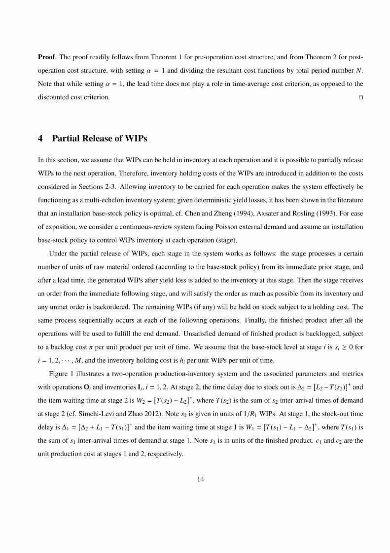
Figure 1 illustrates a two-operation production-inventory system and the associated parameters and metrics
with operations Oi and inventories Ii, i = 1, 2. At stage 2, the time delay due to stock out is ∆2 =[L2−T (s2)
]+ and
the item waiting time at stage 2 is W2 =[T (s2) − L2
]+, where T (s2) is the sum of s2 inter-arrival times of demand
at stage 2 (cf. Simchi-Levi and Zhao 2012). Note s2 is given in units of 1/R1 WIPs. At stage 1, the stock-out time
delay is ∆1 =[∆2 + L1 − T (s1)
]+ and the item waiting time at stage 1 is W1 =[T (s1) − L1 − ∆2
]+, where T (s1) is
the sum of s1 inter-arrival times of demand at stage 1. Note s1 is in units of the finished product. c1 and c2 are the
unit production cost at stages 1 and 2, respectively.
14

I2O2 I1
O1
Demand
Parameters c2, R
2, L
2s2, h
2c1, R
1, L
1s1, h
1
Flow Unit 1/(R1R
2) 1/R
1 1 1
Metrics
Figure 1: Two-Operation Sequence with WIP Inventories and the Associated Parameters
Theorem 3. In a multi-operation production system, for two consecutive operations i and j,
(i) under the pre-operation production cost structure, it is optimal to put operation j before operation i, if and only
if
c j + αL jR jci
RiR j+
(h j
Ri+ αLiπ
)· W(s j, L j) + (hi + π) · B(si, s j, Li, L j)
≤ci + α
LiRic j
RiR j+
( hi
R j+ αL jπ
)· W(si, Li) + (h j + π) · B(s j, si, L j, Li), (31)
where
W(s, L) = αL · E[T (s) − L
]+; (32)
B(s1, s2, L1, L2) = αL1+L2 · E[T (s1) − L1 −
(L2 − T (s2)
)+]+. (33)
(ii) Under the post-operation production cost structure, it is optimal to put operation j before operation i, if and
only if
αL jc j
Ri+ αLi+L jci +
(h j
Ri+ αLiπ
)· W(s j, L j) + (hi + π) · B(si, s j, Li, L j)
≤ αLici
R j+ αLi+L jc j +
( hi
R j+ αL jπ
)· W(si, Li) + (h j + π) · B(s j, si, L j, Li). (34)
(iii) In particular, for both pre- and post-operation cost structures, given everything else the same, those operations
with (1) lower yields, (2) lower processing costs, (3) longer lead times, and (4) lower holding costs should be
placed higher upstream in the system.
15

Proof. Consider the multi-operation sequence X{ j}{i}Y with two operations i and j to be consecutive. We want to
see if the interchange between operations i and j will lessen the expected discounted cost. Since the demands faced
by operations i and j from their downstream operation(s) Y can be treated as a new random variable, it suffices to
consider the two-operation system as illustrated in Figure 1 where the demand is a general random variable.
Under the backlog assumption for unsatisfied demand, for the stationary system, the demand rate satisfies
E[D] = µ = R1R2Q where Q is the average releasing batch size of the raw material per unit of time. Hence, we
have Q = µ/(R1 · R2). Following the idea of tracking product flow, we define the flow unit at each stage to be the
amount sufficient to produce one unit of the finished product. The expected discounted total cost for the stationary
system is decomposed into two parts: (1) CI: the processing/production cost, and (2) CII: inventory related cost
(holding and penalty), which are respectively given as,
CI =µ
R1R2[c2 + α
L2R2c1]; (35)
CII = E[αL2
h2W2µ
R1+ αL1+L2
(h1W1µ + π∆1µ
)]. (36)
Here, the processing cost is assessed at both operations. At O2, the total processing cost is c2 · Q = c2 · µ/(R1 · R2)
under the pre-operation cost structure. Given the backorder assumption for the end product, the average units of
WIPs processed at O1 is µ/R1; otherwise, the end demand will be backlogged infinitely over a long time. In this
case, the processing cost is c1 · µ/R1. The inventory related cost is assessed at both stages as well. In particular,
after lead time L2 at stage 2, the WIPs will be hold on inventory for W2 long and incurs holding cost h2 · (QR2W2).
The released WIPs from stage 2 become the end product after processing at stage 1 with lead time L1. Those µ
units of finished product incur two types of cost: holding cost h1W1 per unit and backorder cost π∆1 per unit.
In what follows, we consider the expected discounted total cost per unit of end demand, V2,1 = (CI + CII)/µ.
By Eqs. (35) and (36), we have
V2,1 =c2 + α
L2R2c1
R1R2+ E[αL2
h2W2
R1+ αL1+L2
(h1W1 + π∆1
)].
Plugging ∆2 =[L2 − T (s2)
]+, W2 =[T (s2) − L2
]+ , ∆1 =[∆2 + L1 − T (s1)
]+ and W1 =[T (s1) − L1 − ∆2
]+ into the
equation above, and using the facts that ∆1 −W1 = ∆2 + L1 − T (s1) and ∆2 −W2 = L2 − T (s2), we rewrite V2,1 as
V2,1 =c2 + α
L2R2c1
R1R2+ αL2
( h2
R1+ αL1π
)E[T (s2) − L2
]++ αL1+L2(h1 + π)E
[T (s1) − L1 − (L2 − T (s2))+
]++ Γ,
where
Γ ≡ Γ(s1, s2, L1, L2) = αL1+L2 · π ·(L1 + L2 − E[T (s1) + T (s2)]
).
16

Therefore, for operation j preceding operation i, the expected discounted total cost per unit of end demand can
be generally expressed as,
V j,i =c j + α
L jR jci
RiR j+
(h j
Ri+ αLiπ
)· W(s j, L j) + (hi + π) · B(si, s j, Li, L j) + Γ(si, s j, Li, L j), (37)
where W(s j, L j) and B(si, s j, Li, L j) are given by Eqs. (32) and (33), respectively.
One may simplify interchange i with j in Eq. (37) to obtain Vi, j. Finally, it is optimal to set operation j pre-
ceding operation i if and only if V j,i ≤ Vi, j, which is simplified to be Eq. (31) after Γ(si, s j, Li, L j) is canceled out
with Γ(s j, si, L j, Li), and hence completes the proof for part (i).
To prove part (ii), we may follow the proof for part (i) and the only difference is the processing/production cost
given by Eq. (35). Here, under post-operation cost structure, the processing/production cost is expressed as
CI = αL2c2µ
R1+ αL1+L2c1µ. (38)
The proof readily follows that for part (i) by replace Eq. (35) with Eq. (38).
To prove part (iii), we only consider pre-operation cost case. The similar argument holds for the post-operation
cost case. Let each operation i be only characterized by Oi = {Ri, ci, Li, hi, si}. To compare two operations Oi and
O j, we consider the variation from only one of those factors while the rest factors are assumed to be identical. In
what follows, we investigate the following cases to see the impact of each of those factors on optimal sequencing.
• Only Ri , R j: then Eq. (31) reduces to
c j + αLR jci + hR j · W(s, L) ≤ ci + α
LRic j + hRi · W(s, L), (39)
where h = hi = h j, L = Li = L j and W(s, L) = W(si, Li) = W(s j, L j). If ci = c j, Eq. (39) holds if and only if
R j ≤ Ri. Namely, O j with a lower yield rate should be put preceding Oi.
• Only ci , c j: then Eq. (31) reduces to Eq. (39). If Ri = R j, Eq. (39) holds if and only if c j ≤ ci. Namely, O j
with a lower processing cost should be put preceding Oi.
• Only Li , L j: then Eq. (31) reduces to
c + αL jRcR2 +
( hR+ αLiπ
)· W(s, L j) + (h + π) · B(s, s, Li, L j)
≤ c + αLiRcR2 +
( hR+ αL jπ
)· W(s, Li) + (h + π) · B(s, s, L j, Li). (40)
17

where h = hi = h j, c = ci = c j and s = si = s j. The above equation holds if and only if L j ≥ Li. We prove
this by contradiction. Assume L j ≤ Li. Then, each of the following holds,
c + αL jRcR2 ≥ c + αLiRc
R2 ; (41)( hR+ αLiπ
)· W(s, L j) ≥
( hR+ αL jπ
)· W(s, Li); (42)
(h + π) · B(s, s, Li, L j) ≥ (h + π) · B(s, s, L j, Li), (43)
where the last equation holds by Eq. (33) given L j ≤ Li and Eq. (42) holds from the following two facts: (a)
W(s, L j) ≥ W(s, Li) given L j ≤ Li; and (b) by Eq. (32)
αLiW(s, L j) = αLi+L j · E[T (s) − L j
]+≥ αLi+L j · E
[T (s) − Li
]+= αL jW(s, Li).
Finally, summing up each terms on both sides of Eqs. (41)-(43) yields a contradiction to Eq. (40). Therefore,
we must have L j ≥ Li.
Namely, operation O j with a longer lead time should be put preceding Oi.
• Only hi , h j: then Eq. (31) reduces to
h j ·[W(s, L) − R · B(s, s, L, L)
]≤ hi ·
[W(s, L) − R · B(s, s, L, L)
], (44)
Note W(s, L) − R · B(s, s, L, L) > 0 by Eqs. (32) and (33). The above holds if and only if h j ≤ hi. Namely,
operation O j with a lower holding cost should be put preceding Oi.
This concludes part (iii) and thus the whole proof is complete. �
Theorem 3 provides the criteria for operation sequencing to minimize the expected discounted cost. The
following corollary shows that the same managerial insight holds for long-run time average cost as well.
Corollary 5. Under a long-run time average cost criterion, pre- or post-operation cost structure, part (iii) of
Theorem 3 still holds, that is, given everything else the same, those operations with (1) lower yields, (2) lower
processing costs, (3) longer lead times, and (4) lower holding costs should be placed higher upstream in the
system.
Proof. The proof readily follows from that of Theorem 3 by setting α = 1 and dividing the resultant cost functions
by the total lead times. �
18

Note that under the time-average cost criterion, the lead time does not affect operations sequencing for the full
release of WIPs, cf. Corollary 4; while for partial release of WIPs, lead time should be considered as an important
factor, cf. Corollary 5. This can be explained by the fact that lead times affect WIPs inventories if they are partially
released, as illustrated by Eqs. (32) and (33).
5 Concluding Remarks
Operations sequencing/re-sequencing can take advantage of flexibility in process design to improve supply chain
efficiency. In this paper, we study operations sequencing in a multi-stage production inventory system with yield
losses for both pre- and post-operation cost structures and both discounted and average cost measures. In the case
of full release of WIPs, we derive the explicit and strong criteria (i.e., almost surely) on sequencing operations
(Theorems 1-2). In the case of partial release of WIPs, we provide explicit criteria (Theorem 3). While the criteria
vary in their explicit forms, they all indicate the same principal, that is, those operations with (1) lower yields, (2)
lower processing costs, (3) longer lead times, and (4) lower holding costs should be placed higher upstream in the
system. Furthermore, the sequencing of two adjustable operations depends not only on these operations themselves
but also on the operations between them. The results can be extended to the cases where different products may
require different sub-sets of operations and the sequence for each product can be optimized individually.
One important assumption of this paper is the deterministic yield, while it is a good approximation for many
practical applications and makes the mathematical analysis tractable, it serves as a starting point of a potentially
much expandable literature where the introduction of random yield may significantly enrich the discoveries. In-
tuitively, under random yield, the optimal operations sequence may depend not only on the expected yields but
also on the yield variability and even the yield distribution. Furthermore, under random yield, the decision of
operations sequence can be intertwined with the dynamic production-inventory decisions. However, inventory
control of multi-echelon inventory systems under random yield is currently an unsolved problem in the literature,
cf. Grosfeld-Nir et al. (2006). We shall leave it and the associated operations sequencing problem to a future
research.
Acknowledgments. The authors thank the Editor-in-Chief, the Associate Editor and two anonymous referees
for their constructive comments and thoughtful suggestions.
19

References
[1] Axsater, S. and K. Rosling (1993), Notes: Installation vs. Echelon stock policies for multilevel inventory
control. Management Science, 39, 1274-1280.
[2] Bard, J. F. and T. A. Feo (1989), Operations sequencing in discrete parts manufacturing. Management Sci-
ence, 35, 249-255.
[3] Boothroyd, H. (1960). Least-cost testing sequence. Journal of the Operational Research Society, 11, 137-138.
[4] Browne, S. and U. Yechiali (1990), Scheduling deterioration jobs on a single processor. Operations Research,
38(3), 495-498.
[5] Chen, F. and Y. Zheng (1994), Lower bounds for multi-echelon stochastic inventory systems. Management
Science, 40(11), 1426-1443.
[6] Cheng, T. and Q. Ding (1998), The complexity of single machine scheduling with release times. Information
Processing Letters, 65(2), 75-79.
[7] Cheng, T., C. Wu, and W. Lee (2008), Some scheduling problems with deteriorating jobs and learning effects.
Computers and Industrial Engineering, 54 (4), 972-982.
[8] Gupta, S. and V. Krishnan (1998), Production family-based assembly sequence design methodology. Institute
of Industrial Engineers Transactions, 30, 933-945.
[9] Gurnani, H., R. Akella and J. Lehoczky (2000), Supply management in assembly systems with random yield
and random demand. Institute of Industrial Engineers Transactions, 32, 701-714.
[10] Grosfeld-Nir, A., Anily, S. and T. Ben-Zvi (2006), Lot-sizing two-echelon assembly systems with random
yields and rigid demand. European Journal of Operational Research, 173(2), 600-616.
[11] Grosfeld-Nir, A. and Y. Gerchak (2004), Multiple lotsizing in production to order with random yields: Review
of Recent Advances. Annals of Operations Research, 126(1-4), 43-69.
[12] Henig, M. and Y. Gerchak (1990), The structure of periodic review policies in the presence of random yield.
Operations Research, 38, 634-642.
[13] Jain, N. and A. Paul (2001), A generalized model of operations reversal for fashion goods. Management
Science, 47, 595-600.
20

[14] Kapuscinski, R. and S. Tayur (1999). Variance vs. standard deviation: variability reduction through operations
reversal. Management Science, 45, 765-767.
[15] Lee, H. L. (1996), Input control for serial production lines consisting of processing and assembly operations
with random yields. Operations Research, 44, 464-468.
[16] Lee, H. and C. S. Tang (1998), Variability reduction through operations reversal in supply chain re-
engineering. Management Science, 44, 162-172.
[17] Lee, H. and C. Yano (1988), Production control in multistage systems with variable yield losses. Operations
Research, 36, 269-278.
[18] Lee, W. (2004), A note on deteriorating jobs and learning in single-machine scheduling problem. Interna-
tional Journal of Business and Economies, 3, 83-89.
[19] Schmidt, C. W. and I. E. Grossmann (1996), Optimization models for the scheduling of testing tasks in new
product development. Industrial Engineering and Chemical Research, 35, 3498-3510.
[20] Schraner, E. and W. Hausman (1997), Optimal production operations sequencing. Institute of Industrial En-
gineers Transactions, 29, 651-660.
[21] Simchi-Levi, D. and Y. Zhao (2012), Performance evaluation of stochastic multi-echelon inventory systems:
a survey. Advances in Operations Research, Volume 2012, 1-34.
[22] Wang, X. and T. Cheng (2008), Single-machine scheduling with deteriorating jobs and learning effects to
minimize the makespan. European Journal of Operational Research, 178(1), 57-70.
[23] Wang, Y. and Y. Gerchak (1996), Periodic review production models with variable capacity, random yield,
and uncertain demand. Management Science, 42, 130-136.
[24] Wein, A. S. (1992), Random yield, rework and scrap in a multistage batch manufacturing environment.
Operations Research, 40, 551-563.
[25] Wu, C., Y. Shiau and W. Lee (2008), Single-machine group scheduling Problems with deterioration consid-
eration. Computers & Operations Research, 35, 1652-1659.
[26] Yan, H., C. Sriskandarajah, S. Sethi and X. Yue (2002), Supply chain redesign to reduce safety stock levels:
sequencing and merging Operations. IEEE Transactions on Engineering Management, 49, 243-257.
21

[27] Yano, C. A. (1986), Controlling production in serial systems with uncertain demand and variable yields.
Technical Report 86-5, Department of Industrial and Operations Engineering, University of Michigan, Ann
Arbor.
[28] Yano, C. A. and H.L. Lee (1995), Lot sizing with random yields: a review. Operations Research, 43, 311-333.
22