Operationalizing the Concept of Neighborhood: Application

to Residential Location Choice Analysis

Jessica Y. Guo* and Chandra R. Bhat

Department of Civil Engineering, University of Texas at Austin, 1 University Station C1761,

Austin, TX 78712-0278, USA

Email: jessica.guo@mail.utexas.edu, bhat@mail.utexas.edu

Phone: 512-471-4535, Fax: 512-475-8744

* Corresponding author

Abstract

In this paper, we explore different conceptualizations to represent neighborhoods in residential

location choice models, and describe three alternative ways for constructing operational units to

represent neighborhoods. In particular, we examine the possibility of using the census units to

represent the hierarchical ‘fixed neighborhood’ definition, and the circular units and network

bands to represent the hierarchical ‘sliding neighborhood’ definition. Overall, the network band

definition is conceptually appealing. It also is marginally superior to the other two operational

representations from a model fit standpoint.

Keywords: Neighborhood; Spatial definition; Residential location choice; Modifiable areal unit

problem

1. Introduction

In the literature relating to urban planning and travel behavior modeling, ‘neighborhood’ is a

widely used and important term. Studies of the housing market investigate what kind of people

live in what kind of neighborhoods (Hunt et al., 1994). Research work on the land-

use/transportation interaction frequently use neighborhood as a synonym for built environment

or land-use. In particular, advocates and skeptics of the ‘New Urbanism’ concept talk about

whether neighborhood design and other characteristics can affect various aspects of travel

behavior (Ewing and Cervero, 2001).

Obviously, any study about neighborhoods is a spatial investigation. Yet, the spatial

definition of neighborhood has received very little attention in the literature. Theoretical studies

of neighborhood effects often use the term neighborhood rather loosely. For instance, New

Urbanism designs tend to focus on the micro scale of four hundred meters (one-quarter mile) or

less. Yet it is not clear on an a priori basis whether residential and travel choice behavior is

influenced by the urban form within small neighborhoods, or over larger areas, or both. On the

other hand, empirical studies of neighborhood effects across many disciplines typically use

census tracts, zip code areas, or transport analysis zones (TAZ) as operational surrogates for

neighborhoods (Sampson et al., 2002; Dietz, 2002). This use of administrative boundaries as

operational units typically has little theoretical foundation and subjects the analysis to the

modifiable areal unit problem (MAUP) (Openshaw, 1984), leading to potentially inaccurate

analytic outcomes and erroneous recommendations for urban policy (see, for example,

Fotheringham and Wong, 1991, and Guo and Bhat, 2004, for more detailed discussions of the

MAUP).

1

So how do we define neighborhoods? Or, how do we measure neighborhood

characteristics and the associated effects? Our simple answer is that we should measure what

matters to people over the area that really matters to people. For example, in the study of

residential location choice, a common hypothesis is that good access to stores is an attractive

neighborhood feature. When examining such a hypothesis, if we define a neighborhood over too

large an area, any spatially concentrated commercial activities would likely be averaged out with

surrounding low-density patterns. Consequently, it would be difficult to associate the

commercial intensity with the choice behavior being studied. Alternatively, if we arbitrarily

define a neighborhood to exclude a commercial center that is in fact easily accessible for a given

household, it would again be difficult to account for the presence of the commercial center in

explaining the residential location choice of that household. Therefore, only when the chosen

definition reflects the decision makers’ perceived neighborhoods can we accurately study the

effect of neighborhoods.

The objective of this paper is to clarify what we, as decision makers and as analysts,

mean by neighborhood and to develop ways of operationalizing the concept of neighborhood.

With residential location choice as the application context, we expand on an earlier work (Guo

and Bhat, 2004) that proposed a hierarchical spatial representation of neighborhoods to examine

neighborhood effects. Our previous study showed the superiority of the hierarchical, multi-scale,

approach over the conventional, single-scale, approach to accommodate the effect of built form,

land use, and other neighborhood attributes. However, the challenge remains regarding how to

exploit the flexibility of using analyst-defined spatial units to appropriately identify the impacts

of neighborhood factors. In this paper, we specifically examine three alternative sets of

operational units for neighborhood definition and embed these spatial representations to study

2

the effects of neighborhood factors on households’ residential location choices. Our results

demonstrate the feasibility of using these operational units of neighborhood, the sensitivity of

modeling outcomes to the choice of spatial units, and the strengths and limitations of the

alternative units.

The remainder of this paper is structured as follows. The next section discusses the

concept of neighborhood, as used in earilier studies. Section 3 provides a background for

residential location choice analysis and discusses the methodological shortcomings in the

conventional approach with regard to the definition of neighborhood. Section 4 briefly reviews

the hierarchical approach proposed in Guo and Bhat (2004) for representing neighborhoods in

residential location choice analysis. Section 5 discusses three different ways to operationalize

the concept of hierarchical neighborhoods. An empirical application of the three ways of

representing neighborhoods is described in Section 6. Finally, Section 7 concludes with a

summary of the contribution of the study.

2. Concept of Neighborhood

Urban social scientists have treated ‘neighborhood’ in much the same way as

courts of law have treated pornography: a term that is hard to define precisely,

but everyone knows it when they see it. (Galster, 2001, p.2111)

Indeed, ‘neighborhood’ is a vague, difficult-to-define, concept. Scholars investigating the

significance of neighborhood for individuals’ behavior and well-being often do not provide the

term with an explicit definition. When spatial definition of neighborhood is required for the

purpose of quantitative analysis, “most social scientists and virtually all studies of neighborhoods

… rely on geographic boundaries defined by the Census Bureau or other administrative

agencies… [which] offer imperfect operational definitions of neighborhoods for research and

3

policy” (Sampson et al., 2002, p.445). This widespread practice suggests that perhaps we don’t

really know ‘it’ − at least not as well as we think − when we see ‘it’. To better understand the

nature of neighborhood, we review and discuss below a collection of approaches for defining the

term. The review is by no means exhaustive, as our focus is on definitions that will bring us

closer to formulate operational units for neighborhoods. The reader is referred to Galster (2001)

for a more extensive survey of the literature.

An area in which neighborhood definition plays an important role is the study of

neighborhood effects, which refers to the neighborhood influences on the well-being and

behavior of families, and often children in particular. A pioneering study (Park, 1916) in the

field points out that cities are generally outlined by their physical geography, natural advantages,

and transportation systems. The processes of human nature then proceed to shape cities through

competitive forces for efficient locations among businesses and individuals. These informal

processes result in the formation of neighborhoods – naturally segregated localities that share

similar sentiments, traditions and history. Followers of this line of thought tend to consider

neighborhoods as discrete, non-overlapping, communities, leading to the common use of

administratively defined zones for analyzing neighborhood effects.

Later, Suttles (1972) argues that, in addition to being the result of free-market

competition, some communities’ identities and boundaries are imposed by outsiders. Suttles also

suggests that neighborhoods are best thought of not as distinct areas of a city, but rather as a

hierarchy of ecological grouping at four levels. At the lowest level is the ‘local networks and the

face-block’, namely, a grouping of residents who share the same local facilities and residential

condition because of their proximity to each other. A neighborhood, defined at this level, is

usually different for each person and is unlikely to have any sharp boundaries. The second level

4

is labeled the ‘defending neighborhood’, defined as “the smallest area which possesses a

corporate identity known to both its members and outsiders”. Its size may vary, but it is

generally large enough to include a complement of establishments (grocery, liquor store, church,

etc.) that people use in their daily round of local movements. The next level, the ‘community of

limited liability’, is typically a construct imposed by external commercial and governmental

interests. Residents may be associated with multiple communities whose boundaries are

fragmented and overlapping. The highest level in the neighborhood hierarchy is the ‘expanded

community of limited liability’. These are large scale community organizations referring to

entire sectors of a city, such as North Austin, whose identity usually arises from government

policies and programs.

Galster (2001) defines a neighborhood as a ‘complex commodity’ that is produced by the

same actors – households, businesses, property owners and local governments – that consume

them. Neighborhood is a bundle of spatially based attributes, including structural,

infrastructural, demographic, class status, tax/public service package, environmental, proximity,

political, social-interactive, and sentimental characteristics. Consistent with Suttle’s (1972)

multi-scale view of neighborhood, Galster argues that the geographical scale across which a

neighborhood attribute varies is often different for different attributes. Consumers’ perceived

delineation of a neighborhood thus depends on the particular neighborhood attributes of interest.

This view is also shared by O’Campo (2003), who contends that the processes operating in the

neighborhood environment are often many and that the ideal geographic units of analysis for

different social processes may not be compatible.

The multi-scale structure of neighborhood can also be viewed as residents having

multiple neighborhood memberships. As different processes (social, educational or religious)

5

unfold, a household can identify its local identity through its residential neighbors, the school the

children go to, its membership in a church, etc. These group memberships lead to spatial

clusters, some of which may be objectively recognizable (such as a school catchment area or a

gated community). In other cases, however, there are often no clear cutoff points for

determining how far social contact or other processes reach. The boundaries for such

neighborhood attributes are subjective and fuzzy. As group memberships of individuals evolve

with their changing roles in the network of social interaction and their stage in life cycle, their

perceptions of neighborhood also change (Horton and Reynolds, 1971). The perception may

also be influenced by race (Lee et al., 1991) and gender (Guest and Lee, 1984). Furthermore, an

individual’s perceived neighborhood also depends on where she or he lives: “an individual living

on the boundary of a census tract probably has more in common with residents of the adjoining

tract than with residents on the far side of his own” (Dubin, 1992, p.435). The concept that no

set of fixed neighborhood boundaries can accurately describe an urban area is referred to as

‘sliding neighborhoods’.

Motivated by the uncertainty about how to construct operational units for neighborhoods

in view of the many factors influencing residents’ perception, Coulton et al. (2001) examine the

residents’ perception through their mental maps. They asked 140 parents of minor children to

draw a map of what they considered as the boundaries of their neighborhoods. The study found

evident discrepancies between resident-defined neighborhoods and census geography. The study

also demonstrated that individuals residing in close proximity and homogenous on race, age and

gender can differ markedly from one another in how they define the physical space of their

neighborhood. This variability renders the task of defining resident-perceived neighborhoods a

very challenging proposition. Coulton et al. conclude by suggesting further research on mental

6

maps of neighborhoods. However, even residents’ hand drawn mental maps, which may be

influenced by neighborhood names or generally acknowledged definitions, may not reflect the

geographic areas that truly affect them (Shinn and Toohey, 2003).

Grannis (1998, 2003) also attempts to construct practical representations of

neighborhoods. He contends that street networks are one of the primary tools populations use to

organize themselves in urban settings and that “the network of tertiary [small, residential-type]

streets give rise to a network of neighborly relations” (Grannis, 1998) (p.1560). In a subsequent

effort, Grannis (2003) models cities as multiple independent ‘islands’ – discontinuous networks

of pedestrian streets that are separated by major thoroughfares. By comparing these islands with

residents’ cognitive maps of their neighborhood, he shows that, while islands circumscribe

residents’ perception of their neighborhoods, residents typically perceive only a portion of their

island as their neighborhood. Like Coulton et al. (2001), he is unable to construct operational

spatial units as close proxies for perceived neighborhoods.

The studies discussed above reflect the well-recognized difficulty in defining a

neighborhood, both at the conceptual and the operational levels. While the question of

neighborhood definition remains to be further explored, the existing literature provides a few

pointers for constructing neighborhood boundaries. First, a neighborhood has a geographical

reference, but its meaning depends on function and domain. The relevant units depend on the

specific process, or the outcome of the process, being studied. Thus, the conventional practice of

using a single definition of spatial units to analyze multiple neighborhood processes (such as the

effects of various neighborhood factors on residential location choice) may lead to spurious

conclusions. Second, an urban region can be viewed as a mix of fixed (objectively recognizable

boundaries such as major roads, geographical barriers and political demarcations) and sliding

7

(subjective boundaries that depend on the characteristics and location of the residents)

neighborhoods. Certain neighborhood processes are related to fixed boundary definitions, while

others are associated with sliding definitions. Third, administratively defined units do not

represent real neighborhoods and thus constitute imperfect operational definitions of

neighborhoods for research and policy. However, census geography in terms of tracts, block

groups and blocks are reasonably consistent with the notion of neighborhood as a nested

ecological structure, where different processes take place at different levels of the structure.

3. Residential Location Choice

The home is where people typically spend most of their time, a common venue for social contact

and, for most people, a major financial and personal investment. One’s choice of residence also

reflects one’s choice of the surrounding neighborhood, which has a significant impact on one’s

well-being and quality of life. The concept of neighborhood and its definition are, therefore,

central to residential location choice analysis.

Residential location choice has long been a multidisciplinary research topic. For urban

and transportation planning, the interest in the causes and consequences of individuals’ choice of

residence arises from the recognition that it is the values, decisions, and actions of the people

who are attracted to certain types of land use patterns that ultimately shape the transportation,

land-use, and urban form. The decision of residential location not only determines the

connection between the household with the rest of the urban environment, but also influences the

household’s activity time budgets and perceived well being. Altering land use characteristics by

itself might not affect the residents’ travel behavior, as expected by proponents of New

Urbanism. Rather, travel characteristics might only change after new residents are attracted by

new land use and move into an area, while old residents who find the land use unsuitable

8

eventually move out (Kitamura et al., 1997; Lund, 2003; Bhat and Guo, 2005). Hence,

understanding the why, who, and where questions associated with residential choices is

important for devising effective spatial policies to manage travel demand.

Over the past four decades, there has been considerable development in the mathematical

modeling of residential activities. A popular modeling approach is based on the discrete choice

formulation pioneered by McFadden (1978). Such a formulation is appealing for residential

choice analysis for at least the following two reasons: First, the decision on residential location

is one that encompasses housing choices as well as the physical and social attributes of the

neighborhood. Based on microeconomic random utility theory, the discrete choice approach

provides a way of understanding how residents trade-off among the wide range of choice factors

that come into play. Second, the discrete choice approach allows the sensitivity to choice

attributes to vary across socio-demographic segments of the population through the inclusion of

interaction terms of spatial characteristics with demographic characteristics of households. The

modeling results can thus help devise urban policies that effectively target specific population

groups.

Of the past discrete choice modeling efforts of residential location, most adopt Lerman’s

(1976) grouped alternatives choice (GAC) model (e.g. Quigley,1985; Gabriel and Rosenthal,

1989; Waddell, 1993 and 1996; Rapaport, 1997; Levine, 1998; Nechyba and Strauss, 1998;

Chattopadhyay, 2000; Sermons and Koppelman, 2001; and Deng, Ross, and Wachter, 2003).

The GAC model is essentially a multinomial logit (MNL) model where the choice alternatives

are the spatial groupings of dwellings, as opposed to the individual dwellings. The probability

that decision maker chooses a dwelling in grouping by is given by: cnP , n c

9

∑=

= C

b

U

U

cnbn

cn

e

eP

1

,,

,

, (1)

where is the utility that decision maker obtains from grouping : cnU , n c

( ) cccncn JXU ln1,, σβ −+′= . (2)

In the above equation, is a vector of observed grouping-specific attributes; cnX , β is a

vector of the model parameters to be estimated; and is used to correct for the grouping

process so that, other conditions being equal, a large grouping would have a higher probability of

being selected than a small grouping. In almost all of the past residential location choice

analyses that have adopted the GAC model, the spatial groupings are interpreted as alternative

neighborhoods of residence and are conceived as commodities with fixed, clearly defined,

boundaries based on administratively defined units such as census tracts (e.g. Lerman, 1975;

Sermons and Koppelman, 2001), school districts (Nechyba and Strauss, 1998), or TAZs

(Waddell, 1996; Deng, Ross, and Wachter, 2003). The neighborhood characteristics are

then constructed accordingly. Such constructs are assumed to provide an accurate representation

of the perceived neighborhood of relevance during the household’s decision making process.

cJ

cnX ,

The GAC modeling approach has a number of limitations. First, by examining

neighborhood attributes over a single definitional configuration of zones, one in fact assumes

that every neighborhood factor operates at one and the same spatial scale. The multi-scale nature

of neighborhood, as discussed in the preceding section, casts serious doubts on the validity of

such an assumption. Second, the use of mutually exclusive administrative zones is a ‘fixed

neighborhoods’ representation, excluding the consideration of the ‘sliding neighborhoods’

concept. Third, the model parameters β are typically interpreted as the effects of the

10

neighborhood attributes on location choice. Yet, as a manifestation of the MAUP, parameter

estimates may differ when different zonal configurations are used. Hence, unless the zones are

coterminous with neighborhoods as perceived by residents, model estimates derived from

arbitrarily defined zones should be interpreted only with respect to these zones and may not

correctly reflect the residents’ choice behavior. This highlights the need to address the

limitations of the GAC approach and to seek more accurate ways of representing residential

neighborhoods in models of residential location choice.

4. The Multi-Scale Logit Model

The use of the GAC model to approximate the ideal disaggregate models (where every

distinguishable dwelling is treated as a distinct choice entity) was a result of the lack of detailed

data for modeling purposes (Lerman, 1976). The same data constraint has also in part

contributed to the use of administrative boundaries as proxy spatial separations for neighborhood

definitions. However, the growing availability of rich, micro-level spatial data and the

proliferation of geographical information systems (GIS) makes it possible to conceive the Multi-

Scale Logit (MSL) model (Guo and Bhat, 2004) as an alternative approach for modeling

residential location choices.

The basic idea of the MSL model is to use multiple definitions of neighborhood within

the same study1. This solution has been implemented in, for example, hierarchical linear models

for studying community psychology (Brodsky, 1999; Duncan et al., 2003), housing price

(Orford, 2002) and, to a limited extent, urban form effect on travel behavior (Boarnet and

1 The MSL model can be considered as a spatial application of the multilevel modeling approach (Goldstein, 1995)

where factors from multiple geographical scales (representing a hierarchical structure of neighborhoods) are

considered in the same analysis.

11

Sarmiento, 1998). To the best of our knowledge, the MSL model of Guo and Bhat (2004)

represents the first implementation of the multi-scale concept of neighborhood in a discrete

choice modeling framework.

The MSL model considers each available dwelling unit as a choice alternative. The

geographic location of an alternative is described by a hierarchy of spatial units . Let

denote the vector of location attributes observed over a spatial unit s (

i iS insX ,

iSs∈ ) for household n of

alternative . The utility experienced by household from choosing dwelling unit i is formally

defined as:

i n

∑∑∈∈

+′=ii Ss

ins

Ss

inss

in XU ,,, εβ . (3)

The error terms, , represent any unobserved effects at each spatial scale. By assuming that

the error terms between different spatial scales are independent of each other, we collapse all the

error terms into one and rewrite the above equation as:

ins

,ε

in

Ss

inss

in

i

XU ,,, εβ +′= ∑∈

. (4)

Furthermore, the error terms are assumed to be independent across alternatives i to allow the

estimation of the β parameters using a MNL structure. Relaxing the independence assumptions

across spatial scales and/or alternatives is an important research avenue for future research2.

The MSL model can be considered as a generalization of Lerman’s GAC model by

allowing the neighborhood variables measured over more than one spatial scale to enter the

utility function. The MSL model structure thus provides a more realistic representation of how

2 If the spatial hierarchical structure follows a fixed-neighborhood definition, then the assumption of independence

across alternatives can be accommodated within the general framework of multi-level models by allowing

correlations across error terms at each spatial level (see, for example, Goldstein, 1995; Hox and Kreft, 1994).

12

neighborhoods are perceived as a hierarchy of ecological structures. Moreover, it allows the

scale, or scales, at which each neighborhood factor operates to be determined endogenously.

That is, the model estimation process reveals not only the neighborhood determinants of

significance to the choice behavior but also the spatial extent of their influence. By interpreting

the parameters with reference to the spatial scale at which they are statistically significant, we

gain insights about the spatial strengths, or cluster sizes, of various neighborhood processes. The

empirical results reported in Guo and Bhat (2004) suggest that the MSL approach yields

statistically superior models than the GAC approach. The analysis was based on spatial

variables measured using census units, thus representing a fixed neighborhood representation.

The findings supported the notion that households of different characteristics have different

spatial cognitions of their neighborhood boundaries. The MSL modeling approach was found to

successfully exploit the modifiability of areal units of measurement to produce richer and more

reliable results.

The other advantage of the MSL model over the GAC model is the capability of allowing

more flexible representations of neighborhoods. This capability is achieved through configuring

the spatial hierarchy, , to represent different hypothetical delineations of neighborhoods based

on the concepts discussed in section 2. For example, can be specified as operational units

representing a hierarchy of ‘fixed neighborhoods’, ‘sliding neighborhoods’, or a mix of both.

However, following this flexibility in neighborhood representation are the questions of how to

appropriately implement the different concepts of neighborhoods and how to determine the ‘best’

implementation for the application at hand. The remainder of this paper represents our first steps

in answering these questions.

iS

iS

13

5. Neighborhood Representations

As discussed earlier, the MSL model structure promotes the use of a hierarchy of spatial units to

capture the effects of neighborhood variables. In this section, we consider three alternative ways

of operationalizing some of the ideas discussed in section 2 to produce spatial units that can be

used in a MSL model to represent residential neighborhoods. Below, we describe each of these

three ways and also discuss their respective merits and drawbacks.

5.1. Census-unit Representation

Since the census data is often the main source of data about the spatial distribution of socio-

demographic variables, one convenient way is to define based on the census geography such

that , where indicates the land parcel on which

dwelling i is located, and , , and are the census block, block-group,

and tract that contain dwelling i , respectively. Figure 1(a) illustrates an example of the census-

based neighborhood representation for a dwelling.

iS

} tract,group-block ,block,parcel{ iiiiiS = iparcel

iblock igroup-block tract i

The census-based definition of is a case of ‘fixed neighborhood’ representation. The

spatial delineations represent objectively defined neighborhood boundaries and, by definition,

the boundaries at each level of the hierarchy are non-overlapping. Since the boundaries of

census units usually follow geographical barriers, streets, and administrative demarcations, the

census-unit representation of neighborhoods is suitable when, and only when, the neighborhood

process being studied is confined to these boundaries. This could be a very restrictive condition,

especially if the analysis is conducted at the relatively micro-scale of census blocks. For

example, if the average property value is computed for a given census block to capture the

market potential of a dwelling unit in that block, then one in fact assumes that the value of any

iS

14

properties in an adjacent block – which could be right across the street from the dwelling unit of

interest – is irrelevant to the analysis. Another drawback of using the census-based

representation is that census units can vary significantly across space in size and shape. For

example, it is highly unlikely that an individual who happens to reside within a census block of

100 km2 would consider the entire block as his/her immediate neighborhood.

5.2. Circular-unit Representation

The use of circles to represent an individual’s perceived neighborhood is motivated by the

concept of ‘sliding neighborhoods’, where the neighborhood boundaries are subjectively defined

by the residents of a dwelling unit. Here, the hierarchy of spatial units is defined as

, where are circular areas of varying radii

demarcated around and centered about each alternative dwelling. The radii of the circular units

may in theory vary for different dwelling units to allow for spatial heterogeneity in perceived

neighborhood extents.

}c, ,c ,parcel{ 1i

kiiiS K= k

iii c,,c ,c 21 K kiii r,,r ,r 21 K

Figure 1(b) shows the circular-unit representation of neighborhoods for the same

dwelling considered in Figure 1(a). The circular representation is a simple, but naïve way of

implementing the sliding neighborhoods concept. It implies that the surrounding environment

within a given distance in all directions is equally important to the decision making process.

Therefore, the circular-unit representation is suitable only if the neighborhood process under

investigation is not confined to natural or artificial barriers that are present within the circular

area.

5.3. Network-band Representation

A more sophisticated way of representing sliding neighborhoods is to take into account the street

network configuration. As suggested by Grannis (1998, 2003) and discussed in section 2 of this

15

paper, residents’ cognitive maps of their neighborhood are at least partially guided by the

(connectivity of) street network in the vicinity of their residence. To implement this idea, we

define , where are network bands constructed for varying

distances . Each network band is a buffer defined around dwelling i such that

the network distance from the dwelling to any point in the buffer is no greater than the pre-

specified value .

}b, ,b ,parcel{ 1i

kiiiS K= k

iii b,,b ,b 21 K

kiii d,,d ,d 21 K k

ib

kid

In practice, one way of constructing the network bands is as follows:

1. Grow a shortest path tree (SPT) from a given dwelling, ; i

2. Truncate the SPT branches to include only the nodes within the pre-specified

distance, , from the dwelling; kid

3. Construct a minimum convex hull that covers the truncated SPT. The resulting

convex hull is the desired network band . kib

The above procedure may be implemented using the GISDK script language provided by

TransCAD, which is a commercial GIS developed especially for transportation applications.

Figure 1(c) shows an example of a network-band generated using a GISDK macro written by us.

Compared to the circular neighborhood representation, the network-bands are

conceptually more appealing because the bands are less likely to contain natural or physical

barriers. Also, while the circular units constructed for a predefined buffer size have identical

shapes and sizes, the network-band corresponding to each dwelling can vary in size and

shape, depending on the density and layout of the surrounding street network. Whereas denser

and grid-like streets lead to smaller and more compact network bands, sparse and cul-de-sec

kib i

16

streets lead to network bands that are larger and more irregular in shape. The degree of variation

in the network bands’ sizes and shapes is, however, not as great as that of the census units.

6. Empirical Application

The three alternative ways described in section 5 for representing neighborhoods have been

implemented and empirically applied to the context of residential location choice modeling. The

empirical application involves estimating three MSL models, each based on one of the three

neighborhood representations. The objectives here are twofold: (1) to examine if, and how, the

three configurations suggest different neighborhood effects on residential location choice

behavior; and (2) compare the statistical fitness of the models to determine their relative

explanatory power. Below, we describe the sample used for model estimation in section 6.1, the

spatial data processing considerations in section 6.2, the variable specifications in section 6.3,

and the estimation results in section 6.4.

6.1. Estimation Sample

The study region we have chosen to empirically apply the three neighborhood representation

methods is the San Francisco Bay Area. The primary data source is the 2000 Bay Area Travel

Survey (BATS) that collected, from members of 15,064 households, detailed information on

individual and household socio-demographic information, employment-related characteristics

and all activity and travel episodes for a two-day period. The dataset also contains the point

geocodes of household residences from which the census block, block group and tract in which

the residence is situated can be identified. The geocodes also enable us to construct concentric

circles and network bands of varying distances around each residence (the sizes of the circles and

bands are described later in section 6.2). From the surveyed households, we randomly select

17

50% of those households living in single-family detached houses. The sub-sampling allows us to

avoid the need of differentiating between housing markets. The final sample contains 4791

households.

Following from the MSL structure, the choice alternatives faced by each household are

the individual dwellings. In theory, the universal choice set in this case comprises all the single-

family detached houses in the Bay area. However, not only are data about all such housing units

in the area unavailable, but it would be computationally impractical to consider them all.

Therefore, we assume that the 4791 residences observed in the sample are a random subset of

such housing opportunities, and consider this as the unobserved choice set faced by each

individual household. We also assume an identically and independently distributed (IID)

structure for the error terms across the alternatives in this universal choice set so that the model

can be consistently estimated with only a subset of the choice alternatives (McFadden, 1978).

The individual choice set constructed for each of the households in the sample includes the

chosen alternative and nine randomly selected non-chosen alternatives.

6.2. Spatial Data Processing

Spatial attributes describing the choice alternatives are derived from a number of data sources, as

listed in Table 1. These sources provide raw data for such spatial units as TAZ and census

blocks and block groups. For our purpose of implementing the alternative neighborhood

representations, we need to first construct the hierarchy of census units, circular units, and

network bands, respectively. Once the spatial units are created, we then overlay the geographic

layer associated with the raw data (the source layer) on to these spatial constructs (the target

layer), followed by appropriate disaggregation and aggregation operations to produce the

neighborhood measures desired for model estimation. It should be noted that, since our source

18

data are already in an aggregate form, the process of disaggregating and aggregating them to the

target layer may introduce further information loss or distortion, with the degree of loss or

distortion depending on the configurations of the source and target polygons. To avoid such

information distortion, one should use source data with the highest spatial resolution.

The construction of the census units is trivial as the Census Bureau provides GIS layers

that readily define the census blocks, block groups, and tracts. The construction of the circular

units and the network bands, however, requires us to first determine the appropriate radii (in the

case of circular units) and band sizes (in the case of network bands). Our selection of radii and

band sizes is based on two considerations. First, in order to reduce the magnitude of information

distortion due to data disaggregation, the circles and bands should be of sizes no smaller than the

census units. The great variation in area size of the census units, however, makes the selection of

distance thresholds difficult. For example, the area size of the 1106 census tracts in the Bay

Area ranges from 0.05 to 1515.07 km2, which are equivalent to circular areas of radius ranging

from 0.13 to 21.97 km. Our second consideration in determining the appropriate sizes for the

circular units and network bands is related to the possibility of high correlations between

neighborhood variables measured at the different scales. To be sure, such correlation effects also

exists among the census units. However, the correlation problem may be worse for the circular

units and network bands if the differential increments between the scales are relatively small.

Based on these two points of considerations, we choose 0.4 km, 1.6 km and 3.2 km as the radii

and band sizes for the three-scale circular-unit and network-bands representations3. The 0.4 km

is slightly greater than the radius of a circle equivalent to the average size of the census blocks

3 The exact measurements of the radii are 0.25, 1.0, and 2.0 mi. Their respective metric equivalents of 0.4, 1.6, and

3.2 km are used in this paper.

19

(which is 0.27 km). It captures the surroundings within what is commonly regarded the average

‘walkable’ distance. The second level of 1.6 km radius is comparable to the size of most census

block-groups and tracts and perhaps caps the ‘walkable’ distance. The third level of 3.2 km

radius is selected to detect neighborhood effects that might operate beyond individuals’ walking

distance. The census units associated with, and the circular units and network bands of the

chosen sizes constructed around, each of the 4791 residential locations in the sample are then

used to compute the various neighborhood variables described in the following section.

6.3. Variable Specification

The following two sets of neighborhood variables are computed for the three sets of spatial

units:

(1) Neighborhood socioeconomic and demographic variables

Several variables are computed to test for the presence of segregation along

various socioeconomic and demographic dimensions. These include the racial

composition variables (percentage of population by race), household type

composition variables (percentage of households by type), tenure composition

variables (percentage of households owning or renting), household income

homogeneity (absolute difference between household income and zonal median

income), and household size homogeneity (absolute difference between

household size and zonal average household size). The racial, household type and

tenure composition variables are further interacted with the corresponding

household racial, family type, and tenure attributes.

(2) Neighborhood design variables

20

A variety of neighborhood design measures were considered for this analysis.

These include density measures (population density, housing density), land-use

composition measures (percentage of coverage by land-use type) and employment

density measures (number of employees per person by sector). We also

considered a more complex measure of land-use diversity defined by:

( ) 5.1414141411 −+−+−+−−= sssssssss TOTITCTRMIX (5)

where is the total area of the unit of analysis sT s ; and , , and are

the acreage of residential, commercial, industrial and other land use types. This

land-use mix index takes a value between 0 and 1, where 1 indicates perfect

mixing of land uses and 0 indicates that the land in a particular area is completely

dedicated to a single land use (Bhat and Gossen, 2004).

sR sC sI sO

Two additional sets of variables are also considered in our MSL models to capture

the effects of regional access, for both commute and non-commute purposes, on the

choice of residential location. These variables are:

(1) Commute-related variables

Based on the residents’ work and alternative residential TAZ locations, we extract

from the level-of-service data the auto commute times and costs, which are then

interacted with individual work status, gender, ethnicity, and income variables.

(2) Regional accessibility

A residential location’s attractiveness depends not only on its immediate

surroundings, but also how it relates spatially to the rest of the urban area. This is

the motivation for considering regional accessibility measures for shopping,

recreational, and employment activities. We compute the accessibility measures

21

as NdRAN

jijj

Shopi ⎟⎟

⎠

⎞⎜⎜⎝

⎛= ∑

=1, NdEA

N

jijj

Empi ⎟⎟

⎠

⎞⎜⎜⎝

⎛= ∑

=1, and NdVA

N

jijj

ci ⎟⎟

⎠

⎞⎜⎜⎝

⎛= ∑

=1

Re

where , and denote the shopping, employment and recreational

accessibility indices, respectively, for TAZ ; , and are the number of

retail employment, number of basic employment and vacant land acreage in TAZ

, respectively; is the distance between zones i and . Due to data

constraints, these zonal accessibility measures are used in our analysis as proxy

for point-to-region accessibility measures for each observed residence. Large

values of the accessibility measures indicate more opportunities for activities in

close proximity of that residence, while small values indicate residences that are

spatially isolated from such opportunities.

EmpiA c

iARe ShopiA

i jR jE jV

i ijd j

6.4. Estimation Results

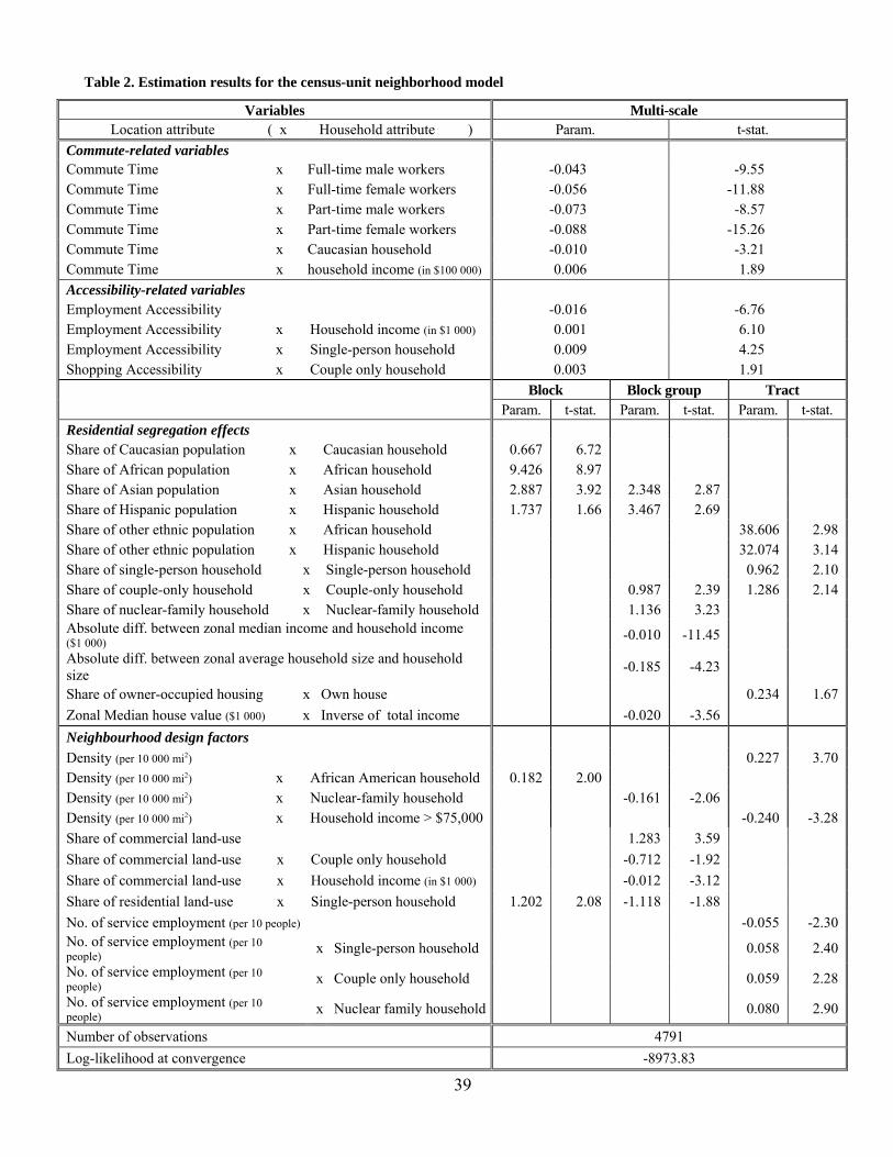
We arrived at the final specification for each of the three models based on a systematic process

of testing and eliminating variables found to be statistically insignificant. The specification was

also guided by parsimony and intuitive considerations, and the results from earlier studies. The

final specifications are presented in Table 2 (census-unit representation), Table 3 (circular-unit

representation) and Table 4 (network-band representation). The results are discussed below by

variable group. Overall, the three models are consistent in the signs of the parameter estimates.

The final specifications differ in the presence and the absence of certain variables and the spatial

level at which the variables are significant.

22

Commute-related variables

The three models are most comparable in terms of the parameter estimates (both in sign

and magnitude) associated with commute time. All models reveal that households tend to locate

themselves closer to the work locations of the workers in the household. In particular,

households locate themselves close to the workplace of the female workers in the household.

This gender disparity supports the household responsibility hypothesis (Sermons and

Koppelman, 2001). A similar higher responsibility hypothesis may be the underlying cause for

the greater commute time effect on part-time workers relative to full-time workers. The racial

disparity in commute sensitivity suggests greater spatial job-housing mismatch for non-

Caucasians compared to Caucasians. The positive sign associated with the interaction of

commute time and income may be a reflection of the willingness of higher income earners to

travel further in exchange for better housing quality.

Accessibility-related variables

The three models also have similar estimates for the sensitivity to employment

accessibility. Taken together with the parameter on the interaction term between employment

accessibility and income, the results indicate that households earning an annual income greater

than $16 000 (in the census-unit model) or $12 000 (in the circular-unit model) or $8 000 (in the

network-band model) tend to locate themselves near employment centers even after the direct

accessibility to work locations has been accounted for. Single-person households are also found

to locate in closer proximity to regional employment opportunities than other types of

households. The effect of regional shopping accessibility is different for the models. While the

census-unit model suggests that, compared to other household types, couple-only households

tend to locate in areas with good access to shopping opportunities, the other two models do not

23

suggest any difference in sensitivity to shopping accessibility across household types.

Recreation accessibility measures were introduced into the utility function during the estimation

process, but were not found to impact residential choice.

Residential segregation effects

A consistent finding in all models is the evidence of residential segregation across a

number of dimensions. As indicated by the magnitude of the parameter estimates, African-

Americans are the most segregated group, while Hispanics and Asians are segregated to a lesser

degree – this finding is in agreement with the national demographic trend found in Iceland et al.

(2002). The results essentially indicate that African-Americans and Hispanics are more likely to

integrate with other minority groups compared to Caucasian and Asians. It is also interesting

that, despite the common impression of strong Black-White segregation, the coefficient

associated with the share of Caucasian population interacted with Caucasian household is

relatively smaller than the respective coefficient associated with the share of African-

American/Asian/Hispanic population interacted with African-American/Asian/ Hispanic

household. This perhaps indicates that the Caucasians in the Bay area have a relatively high

tolerance for the presence of the other population groups as a whole in their neighborhoods.

Evidence of strong racial segregation is a common finding in past studies of residential

location choice. What past studies have not been able to reveal is the differential spatial extents

of the racial clustering behavior. Our estimation results show that the size of racial clusters does

vary for different racial groups and that different neighborhood definitions suggest different

cluster sizes. In Tables 3 and 4, almost all the racial clustering variables are significant at, and

only at, the 0.4 km direct/network distance level, with the exception being the aggregation of the

‘other’ ethnic population with African-American households. This suggests that racial clusters

24

are generally of 0.4 km in radius. The census-unit model in Table 2, however, tells a different

story. The aggregation among Caucasians and among African-Americans is prominent in census

blocks only; whereas the aggregation among Asians and among Hispanics is found in both

census blocks and block-groups. Also, the integration of African-Americans and of Hispanics

with the other minority groups is found only at the tract level. This difference in spatial scales of

racial segregation between the two models is perhaps a result of the MAUP, the variation in the

sizes of census units, or other factors that require further research to uncover.

The household structure-related segregation effects suggest that a household tends to

locate in an area with a high proportion of other households with a similar household structure

and household size as their own. Table 2 suggests the presence of clustering among couple-only

and nuclear-family households at the census block-group level, and clustering among single-

person and couple-only households at the census tract level. Tables 3 and 4 both show that the

cluster size of single-person households (1.6 km) is higher than that of the other household types

(0.4 km). In addition to segregation by race and household structure, households are found to

locate near other households of similar income level, household size, and residential tenure

status. Again, the observed inconsistency between the three models regarding the clustering size

of households along various demographic and socio-economic dimensions calls for further

research.

Neighborhood design factors

The consistency of the neighborhood design parameters among the three models is very

mixed. Density and density interacted with nuclear-family households are significant in all three

models, but show different spatial extents of influence. The census-unit model implies that

households generally locate in census tracts of high population density, but nuclear-families are

25

less likely to location in census block-groups of high density. The circular-unit and network-

band models indicate that high population density within close proximity (0.4 km in terms of air

or network distance) of households’ residence generally has a positive influence on households’

residential location choice. However, population density has a negative influence on nuclear-

family households, and the extent of this influence is within a 1.6 km radius of their residence

(the circular-unit model) or 3.2 km network distance from their residence (the network-band

model). In the census-unit model, density is also found to have an additional positive effect on

African-Americans and a negative effect on high-income households. In the network-band

model, density also has a negative effect on high-income households (annual income above $114

000).

Of the several land-use composition variables and their interaction terms with household

characteristics, only the share of the commercial land-use variable and the share of commercial

land-use interacted with household income variable are significant in both census-unit and

circular-unit model specifications. Taken together, the parameters suggest that the attractiveness

of local access (within the same census block-group, or within the 1.6 km radius neighborhood)

to stores diminishes as household income increases. In addition, as suggested by the census-unit

model but not the circular-unit model, couple-only households are less likely to location in

census block-groups with high commercial land-use than other types of households. The census-

unit model also indicates different effects of residential land-use at two spatial scales on single-

only households. On the other hand, the network-band model suggests that, compared to lower-

income households, high income households are more likely to locate themselves in residential-

oriented areas (within 1.6 km of the residence). Also, couple-only households tend to locate

themselves in areas with less open space then other types of households.

26

Of the employment density variables tested, only the service employment density

variable has an influence on residential choice decisions. The census-unit model indicates that,

on the one hand, nuclear-family, couple-only and single-only households are more likely to

locate in census tracts with high service employment density, with the degree of likelihood being

highest for nuclear-families and lowest for single-only households; but on the other hand,

households other than these three types are less likely to locate in such tracts. The effects of

service employment density, however, are not evident in the circular-unit model nor the network-

band model.

It is surprising that the land-use mix parameter, either by itself or through interaction with

the various household characteristics, does not appear to be a significant factor in the census-unit

model. This suggests that, after the access to particular types of land-use (commercial) or

amenity (service) is accounted for, mixed land-use does not have influence on residential

location choice behavior. With the network-band model, however, we find evidence supporting

the hypothesis that households with no car are more likely to reside in mixed land-use

environment. The circular-unit model also suggests effects of land-use mix, measured within 1.6

km network distance, on residential location choice. Measured within a 3.2 km radius around the

residences, heterogeneous land-use composition has a positive effect on households with none or

one car, and a negative effect on households with young children. These effects appear to be

intuitive.

Measures of fit

Since the number of variables present in the final specifications is different between the

census-unit model and the circular-unit model, the log-likelihood ratios are not directly

comparable. Instead, we compare the goodness-of-fit of the two models using the adjusted

27

likelihood ratio (ALR). The values of the ALR for the census-unit, circular-unit, and network

band models are 0.183, 0.183, 0.184, respectively. That is, statistically speaking, the network-

band model is found to be superior to the other two models. The differences in model goodness-

of-fits are, however, quite small and not statistically significantly different based on non-nested

likelihood ratio tests (see Ben-Akiva and Lerman, 1985, for a discussion of non-nested

likelihood ratio tests).

7. Summary and Conclusions

The ‘neighborhood’ is a key concept in urban study. Its attributes can be observed and

accurately measured only after a location has been specified and a space of relevance been

demarcated. In this study, we investigate the spatial definition problem of neighborhood in the

context of residential location choice analysis. From past research efforts aimed at

conceptualizing the nature of neighborhood, we learn that neighborhood is intrinsically

hierarchical and is continuously shaped by the infrastructure and the many ecological and social

processes that take place in the urban environment. The hierarchical organization and the spatial

boundaries of neighborhood are very much domain dependent. In certain contexts they can be

described by objectively recognizable spatial delineations while, in other situations, they are

constructed by individuals’ perception. This dynamic nature of neighborhood renders the

popular grouped alternatives modeling approach methodologically flawed. By not appropriately

considering neighborhood attributes over the area that really matters to the decision makers,

these past modeling efforts produce biased parameter estimates that lead to erroneous

interpretations and ineffective policies.

We contend that, with the increasing availability of micro-level spatial data and the

proliferation of GIS, researchers should re-examine the conventional practice and consider the

28

more general, and behaviorally more realistic, MSL modeling approach. The MSL model serves

as a useful tool for uncovering the appropriate spatial structure to best represent neighborhood

for a given study context. Our earlier work (Guo and Bhat, 2004) showed that, at least in the

context of residential location choice analysis, the hierarchical nature of the MSL model

outperforms the single-level model both conceptually and statistically. The MSL model is

especially valuable in its ability to allow the spatial scale of relevance for each variable to be

determined endogenously.

In this paper, we explore different conceptualizations of neighborhoods and describe

three alternative ways for constructing operational units to represent neighborhoods. In

particular, we examine the possibility of using the census units to represent the hierarchical

‘fixed neighborhood’ definition, and circular units and network bands around housing units to

represent the hierarchical ‘sliding neighborhood’ definition. Each of these three neighborhood

representations has its conceptual merits and drawbacks. The fact that the boundaries of census

units often follow the street network makes the units a good candidate for studying the

neighborhood factors whose influence are perceived to differ from one street block to the other.

However, the same quality also makes the census unit unsuitable for studying other types of

neighborhood processes. Another major drawback is that the census units vary greatly in size

and shape, rendering it difficult to interpret the associated parameters. One the same note, the

distance-based units (circular units and network bands) provide much more tangible indication of

the spatial extents of the neighborhood factors’ influence. Moreover, since the network bands

are constructed based on the street network, they have the desirable quality of including major

natural/physical barriers in their boundary definition.

29

Our empirical application of the three neighborhood representation methods in studying

households’ residential location choices showed that the network band representation is

statistically, but not significantly, superior to the other two representations. A number of

additional conclusions can be drawn from the empirical results. First, the three models are

generally consistent in the signs and magnitudes of the parameter estimates relating to the

commute-related and the regional accessibility variables. For the other variables considered in

the analysis, the models differ in the variables that are significant and the spatial scale at which

these variables are significant. Second, for parameters that are found to be significant, they tend

to have the same sign but their respective values can differ up to 300%. Third, all three models

suggest that the social-economic and demographic composition variables have significantly

smaller spatial extent of influence than the land-use variables. The aforementioned findings can

perhaps explain why previous residential choice models utilizing the GAC approach sometimes

fail to provide empirical evidence for certain intuitive hypotheses about the impact of

neighborhood characteristics on residential utility.

The current study has demonstrated the feasibility, and the potential benefits, of breaking

away from utilizing administrative zones in residential location choice analysis, as well as other

activity-based analyses that involve neighborhood variables. Yet, it does not necessarily answer

the question of what operational units are most suitable for analyzing neighborhood variables. In

fact, this study represents only the beginning of an inquiry into that question. Future research

along this line of inquiry may include the following: (1) empirically applying and comparing the

alternative spatial representations based on disaggregate data (as opposed to, for example, land

use data at the TAZ level) to more accurately assess their empirical explanatory power; (2)

devising alternative hierarchical representations of neighborhoods to incorporate both of (or the

30

merits of both) the fixed- and sliding-neighborhood concepts; (3) examining the appropriate

scales of analysis to successfully identify the effects of neighborhood variables while avoiding

the effects of multi-colinearity; (4) designing surveys to collect data that will help identify

respondents’ perceived neighborhood boundaries.

Acknowledgement

We would like to thank Professor Harvey Miller for his suggestion on defining

neighborhoods based on network distance and an anonymous individual for constructive

comments on an earlier version of the paper.

31

Reference

Ben-Akiva, M., Lerman, S. R., 1985. Discrete Choice Analysis: Theory and Application to

Travel Demand. MIT Press, Cambridge, Massachusetts.

Bhat, C.R., Gossen, R., 2004. A mixed multinomial logit model analysis of weekend recreational

episode type choice. Transportation Research Part B 38(9), 767-787.

Bhat, C.R. and Guo, J.Y., 2005. A comprehensive analysis of built environment characteristics

on household residential choice and auto ownership levels. Technical paper, Department

of Civil Engineering, The University of Texas at Austin, July 2005.

Boarnet , M .G., Sarmiento, S., 1998. Can land-use policy really affect travel behavior? A study

of the link between non-work travel and land-use characteristics. Urban Studies 35(7),

1155-1169.

Brodsky, A., O’Campo, P., Aronson, R., 1999. PSOC in community context: multilevel

correlates of a measure of psychological sense of community in low income, urban

neighborhoods. Journal of Community Psychology 27, 659-680.

Chattopadhyay, S., 2000. The Effectiveness of McFadden’s Nested Logit Model in Valuing

Amenity Improvement, Regional Science and Urban Economics 30, 23-43.

Coulton, C.J., Korbin, J., Chan, T., Su, M., 2001. Mapping residents’ perceptions of

neighborhood boundaries: A methodological note. American Journal of Community

Psychology 29(2), 371-383.

Deng, Y., Ross, S.L., Wachter, S.M., 2003. Racial Differences in Homeownership: The Effect of

Residential Location, Regional Science and Urban Economics 33, 517-556.

Dietz, R.D., 2002. The estimation of neighborhood effects in the social sciences: An

32

interdisciplinary approach. Social Science Research 31, 539-575.

Dubin, R.A., 1992. Spatial Autocorrelation and Neighborhood Quality. Regional Science and

Urban Economics 22, 433-452.

Duncan, T.E., Duncan, S.C., Okut, H., Strycker, L.A., Hix-Small, H., 2003. A multilevel

contextual model of neighborhood collective efficacy. American Journal of Community

Psychology 32(3/4), 245-252.

Ewing, R., Cervero, R., 2001. Travel and the built environment – synthesis. Transportation

Research Record 1780, 87-114.

Fotheringham, A.S., Wong, D.W.S., 1991. The modifiable areal unit problem in multivariate

statistical analysis. Environment and Planning A 23, 1025-1044.

Galster, G.C., 2001. On the nature of neighborhood. Urban Studies 38(12), 2111-2124.

Gabriel, S.A., Rosenthal, S.S., 1989. Household Location and Race: Estimates of a Multinomial

Logit Model, The Review of Economics and Statistics 17 (2), 240-249.

Goldstein, H., 1995. Multilevel Statistical Models. Edward Arnold, London.

Grannis, R., 2003. Islands in the city: Social networks and street networks. Working paper,

Department of Sociology, University of California, Los Angeles.

Grannis, R., 1998. The importance of trivial streets: Residential streets and residential

segregation. American Journal of Sociology 103(6), 1530-1564.

Guest, A.M., Lee, B.A., 1984. How urbanites define their neighborhoods. Population and

Environment 7(1), 32-56.

Guo, J.Y., Bhat, C.R., 2004. Modifiable areal units: a problem or a matter of perception?

Transportation Research Record, forthcoming.

33

Horton, F.E., Reynolds, D.R., 1971. Effects of urban spatial structure on individual behavior.

Economic Geography 47(1), 36-48.

Hox, J.J., Kreft, I.G., 1994. Multilevel analysis methods, Sociological Methods and Research,

22, 283-299.

Hunt, J.D., McMillan, J.D.P., Abraham, J.E., 1994. Stated Preference Investigation of Influences

on Attractiveness of Residential Locations. Transportation Research Record 1466, 79-87.

Iceland, J., Weinberg, D.H., Steinmetz, E., 2002. Racial and Ethnic Residential Segregation in

the United States: 1980-2000. U.S. Census Bureau, Census Special Report, CENSR-3,

US Government Printing Office, Washington, DC.

Kitamura, R., Mokhtarian P.L., Laidet, L., 1997. A micro-analysis of land use and travel in five

neighborhoods in the San Francisco Bay Area. Transportation 24(2), 125-158.

Lee, B.A., Campbell, K.E., Miller, O., 1991. Racial differences in urban neighboring.

Sociological Forum 9(3), 525-550.

Levine, J., 1998. Rethinking Accessibility and Jobs-Housing Balance, Journal of American

Planning Association 64(2), 133-149.

Lerman, S.R., 1976. Location, Housing, Automobile Ownership and Mode to Work: A Joint

Choice Model. Transportation Research Record 610, 6-11.

Lund, H., 2003. Testing the claims of New Urbanism. APA Journal 69(4), 414-429.

McFadden, D., 1978. Modeling the Choice of Residential Location. In: Karlqvist, A. et al. (Eds),

Spatial Interaction Theory and Planning Models. Amsterdam: North Holland Publishers.

Nechyba, T.J., Strauss, R.P., 1998. Community Choice and Local Public Services: A Discrete

Choice Approach, Regional Science and Urban Economics 28, 51-73.

34

O’Campo, P., 2003. Invited commentary: Advancing theory and methods for multilevel models

of residential neighborhoods and health. American Journal of Epidemiology 157(1), 9-13.

Openshaw, S., 1984. Concepts and Techniques in Modern Geography: Number 38 - The

Modifiable Areal Unit Problem. Norwick: Geo Books.

Orford, S., 2002. Valuing locational externalities: A GIS and multilevel modeling approach.

Environment and Planning B: Planning and Design 29, 105¯127.

Park, R., 1916. Suggestions for the Investigations of Human Behavior in the Urban Environment.

American Journal of Sociology 20(5), 577-612.

Quigley, J.M., 1985. Consumer Choice of Dwelling, Neighborhood and Public Services.

Regional Science and Urban Economics 15, 41-63.

Rapaport, C., 1997. Housing Demand and Community Choice: An Empirical Analysis, Journal

of Urban Economics 42, 243-260.

Sampson, R.J., Morenoff, J.D., Gannon-Rowley, T., 2002. Assessing ‘neighborhood effects’:

Social processes and new directions in research. Annual Reviews in Sociology 28, 443-

478.

Sermons, M.W., Koppelman, F.S., 2001. Representing the differences between female and male

commute behavior in residential location choice models. Journal of Transport Geography

9(2), 101-110.

Shinn, M., Toohey, S.M., 2003. Community contexts of human welfare. Annual Reviews in

Psychology 54, 427-459.

Suttles, G.D., 1972. The Social Construction of Communities. Chicago: University of Chicago

Press.

35

Waddell, P., 1996. Accessibility and Residential Location: The Interaction of Workplace,

Residential Mobility, Tenure, and Location Choices, presented at the Lincoln Land

Institute TRED Conference. [http://www.odot.state.or.us/tddtpan/modeling.html]

Waddell, P., 1993. Exogenous workplace choice in residential location models: Is the assumption

valid?. Geographical Analysis 25, 65-82.

36

LIST OF TABLES

TABLE 1 Spatial variables considered in the residential choice models

TABLE 2 Estimation results for the census-unit neighborhood model

TABLE 3 Estimation result for the circular-unit neighborhood model

TABLE 4 Estimation result for the network-band neighborhood model

LIST OF FIGURES

FIGURE 1 Alternative ways of representing perceived neighborhood

37

38

TABLE 1. Spatial variables considered in the residential choice models

Data source Spatial level at which data is available Variables considered

Bay Area Metropolitan Transportation Commission

Transport analysis zone • Number of employment by sector (retail, wholesale, service, manufacturing, agriculture, and other)

• Land-use acreage by purpose (residential, office, retail, and vacant)

Bay Area Metropolitan Transportation Commission

Transport analysis zone Inter-zonal • Distances • Peak and off-peak travel times and costs by travel

mode (car, shared ride, transit mode by both walk access, and transit mode by drive access)

Census block • Number of households • Population • Land/water area • Number of people by ethnicity (non-Hispanic

Caucasian, African American, Asian, Hispanic, and other)

Census 2000 population and housing data summary file 1 (SF1)

Census block-group • Median household income • Average household size • Number of housing units by size (single-family

detached, apartments, etc) • Median housing value • Number of households by income quartiles

39

Table 2. Estimation results for the census-unit neighborhood model

Variables Multi-scale Location attribute ( x Household attribute ) Param. t-stat.

Commute-related variables Commute Time x Full-time male workers -0.043 -9.55 Commute Time x Full-time female workers -0.056 -11.88 Commute Time x Part-time male workers -0.073 -8.57 Commute Time x Part-time female workers -0.088 -15.26 Commute Time x Caucasian household -0.010 -3.21 Commute Time x household income (in $100 000) 0.006 1.89 Accessibility-related variables Employment Accessibility -0.016 -6.76 Employment Accessibility x Household income (in $1 000) 0.001 6.10 Employment Accessibility x Single-person household 0.009 4.25 Shopping Accessibility x Couple only household 0.003 1.91 Block Block group Tract Param. t-stat. Param. t-stat. Param. t-stat. Residential segregation effects Share of Caucasian population x Caucasian household 0.667 6.72 Share of African population x African household 9.426 8.97 Share of Asian population x Asian household 2.887 3.92 2.348 2.87 Share of Hispanic population x Hispanic household 1.737 1.66 3.467 2.69 Share of other ethnic population x African household 38.606 2.98 Share of other ethnic population x Hispanic household 32.074 3.14 Share of single-person household x Single-person household 0.962 2.10 Share of couple-only household x Couple-only household 0.987 2.39 1.286 2.14 Share of nuclear-family household x Nuclear-family household 1.136 3.23 Absolute diff. between zonal median income and household income ($1 000) -0.010 -11.45 Absolute diff. between zonal average household size and household size -0.185 -4.23

Share of owner-occupied housing x Own house 0.234 1.67 Zonal Median house value ($1 000) x Inverse of total income -0.020 -3.56 Neighbourhood design factors Density (per 10 000 mi2) 0.227 3.70 Density (per 10 000 mi2) x African American household 0.182 2.00 Density (per 10 000 mi2) x Nuclear-family household -0.161 -2.06 Density (per 10 000 mi2) x Household income > $75,000 -0.240 -3.28 Share of commercial land-use 1.283 3.59 Share of commercial land-use x Couple only household -0.712 -1.92 Share of commercial land-use x Household income (in $1 000) -0.012 -3.12 Share of residential land-use x Single-person household 1.202 2.08 -1.118 -1.88 No. of service employment (per 10 people) -0.055 -2.30 No. of service employment (per 10 people) x Single-person household 0.058 2.40 No. of service employment (per 10 people) x Couple only household 0.059 2.28 No. of service employment (per 10 people) x Nuclear family household 0.080 2.90

Number of observations 4791 Log-likelihood at convergence -8973.83

40

Table 3. Estimation result for the circular-unit neighborhood model

Variables Multi-scale Location attribute ( x Household attribute) Param. t-stat.

Commute-related variables Commute Time x Full-time male workers -0.042 -9.28 Commute Time x Full-time female workers -0.055 -11.74 Commute Time x Part-time male workers -0.073 -8.53 Commute Time x Part-time female workers -0.087 -15.09 Commute Time x Caucasian household -0.011 -3.37 Commute Time x household income ($100 000) 0.006 1.65 Accessibility-related variables Employment Accessibility -0.011 -4.98 Employment Accessibility x Household income ($1 000) 0.001 4.85 Employment Accessibility x Single-person household 0.008 5.01

R = 0.4 km R = 1.6 km R = 3.2 km

Param t-stat. Param t-stat. Param t-stat. Residential segregation effects Share of Caucasian population x Caucasian household 0.794 6.45

Share of African population x African household 10.544 7.41

Share of Asian population x Asian household 5.209 11.71

Share of Hispanic population x Hispanic household 5.236 5.89

Share of other ethnic population x African household 50.792 4.18

Share of other ethnic population x Hispanic household 32.357 3.34 Share of single-person household x Single-person household 1.285 2.84

Share of couple-only household x Couple-only household 2.077 5.78

Share of nuclear-family household x Nuclear-family household 1.003 2.18

Absolute difference between zonal median income and household income (in $1 000) -0.011 -12.11

Absolute difference between zonal average household size and household size -0.221 -4.10

Share of owner occupied housing x Own house 0.617 3.31 Zonal Median housing value ($1 000) x Inverse of household

income -0.024 -3.89

Neighbourhood design factors Density (per 10 000 mi2) 0.150 3.11

Density (per 10 000 mi2) x Nuclear-family household -0.237 -2.21

Share of commercial land-use 1.108 2.45

Share of commercial land-use x Household income ($1 000) -0.011 -2.040

Land-use mix x Own no cars 1.944 1.63

Land-use mix x Own 1 car 0.553 1.98

Land-use mix x Presence of kids in household -0.576 -2.02

Number of observations 4791

Log-likelihood at convergence -8984.32

41

Table 4. Estimation result for the network-band neighborhood model

Variables Multi-scale Location attribute ( x Household attribute) Param. t-stat.

Commute-related variables Commute Time x Full-time male workers -0.042 -9.49 Commute Time x Full-time female workers -0.055 -11.93 Commute Time x Part-time male workers -0.072 -8.63 Commute Time x Part-time female workers -0.087 -15.13 Commute Time x Caucasian household -0.011 -3.31 Commute Time x household income ($100 000) 0.006 1.87 Accessibility-related variables Employment Accessibility -0.009 -4.47 Employment Accessibility x Household income ($1 000) 0.001 4.17 Employment Accessibility x Single-person household 0.008 4.93

R = 0.4 km R = 1.6 km R = 3.2 km

Param t-stat. Param t-stat. Param t-stat. Residential segregation effects Share of Caucasian population x Caucasian household 0.769 6.41

Share of African population x African household 10.266 7.41

Share of Asian population x Asian household 5.151 11.71

Share of Hispanic population x Hispanic household 5.024 5.76

Share of other ethnic population x African household 49.832 4.12

Share of other ethnic population x Hispanic household 18.760 2.70 Share of single-person household x Single-person household 1.491 3.17

Share of couple-only household x Couple-only household 1.707 5.15

Share of nuclear-family household x Nuclear-family household 1.110 2.69

Absolute difference between zonal median income and household income (in $1 000) -0.010 -11.84

Absolute difference between zonal average household size and household size -0.184 -4.04

Share of owner occupied housing x Own house 0.485 3.01 Zonal Median housing value ($1 000) x Inverse of household

income -0.028 -3.91

Neighbourhood design factors Density (per 10 000 mi2) 0.151 2.87

Density (per 10 000 mi2) x Nuclear-family household -0.274 -2.46

Density (per 10 000 mi2) x High income households -0.110 -1.64

Share of residential land-use -0.360 -2.41

Share of residential land-use x Household income ($1 000) 0.003 2.00

Share of open space x Couple-only households -0.259 -2.28

Land-use mix x Own no cars 2.009 2.16

Number of observations 4791

Log-likelihood at convergence -8974.07

Figure 1. Alternative ways of representing perceived neighborhood

(a) Fixed neighborhood representation based on census units

(b) Sliding neighborhood representation based on circular-units

(c) Sliding neighborhood representation based on network bands

42