Open Source implementations of encoding

algorithms for video distribution in the

HTML5 era

Federico Pistono

Dissertation committee:

doctor Davide Quaglia

University of Verona

Department of computer science

September 25, 2009

Copyright c©2009 by Federico PistonoSome Rights Reserved

This work is licensed under the terms of the Creative Commons Attri-bution – Noncommercial – Share Alike Works 3.0 license. The license isavailable at http://creativecommons.org/licenses/by-nc-sa/3.0/

Attribution – Noncommercial – Share Alike Works

You are free:

To Share – to copy, distribute and transmit the work

Under the following conditions:

Attribution – You must attribute the work in the mannerspecified by the author or licensor (but not in any way thatsuggests that they endorse you or your use of the work).

Noncommercial – You may not use this work for com-mercial purposes.

Share Alike –If you alter, transform, or build upon thiswork, you may distribute the resulting work only under thesame or similar license to this one.

With the understanding that:

Waiver – Any of the above conditions can be waived if you get permissionfrom the copyright holder.

Other Rights – In no way are any of the following rights affected by thelicense:

• Your fair dealing or fair use rights;

• The author’s moral rights;

i

• Rights other persons may have either in the work itself or in how thework is used, such as publicity or privacy rights.

Notice – For any reuse or distribution, you must make clear to others thelicense terms of this work. The best way to do this is with a link to the webpage http://creativecommons.org/licenses/by-nc-sa/3.0/.

ii

To my friends and familyfor their warmth

and supportand to the Open Source community

who gave everything,without asking

for anything in return.

iii

Contents

1 The state of the art and how we got here 21.1 Video quality . . . . . . . . . . . . . . . . . . . . . . . . . . . 51.2 MPEG - Moving Picture Experts Group . . . . . . . . . . . . 6

2 Advanced Video Coding and OSS 92.1 An Open Source video codec: x264 + FFmpeg . . . . . . . . . 112.2 Comparison of Proprietary and Open Source Software . . . . . 12

3 Ogg Theora 193.1 Technical specification . . . . . . . . . . . . . . . . . . . . . . 213.2 Theora and the Web . . . . . . . . . . . . . . . . . . . . . . . 223.3 Ogg Theora vs. x264 . . . . . . . . . . . . . . . . . . . . . . . 223.4 Ogg Theora - YouTube subjective comparison . . . . . . . . . 23

3.4.1 Methodology . . . . . . . . . . . . . . . . . . . . . . . 243.4.2 Results . . . . . . . . . . . . . . . . . . . . . . . . . . . 25

3.5 Ogg Theora - YouTube SSIM comparison . . . . . . . . . . . . 273.5.1 Methodology . . . . . . . . . . . . . . . . . . . . . . . 273.5.2 Results . . . . . . . . . . . . . . . . . . . . . . . . . . . 30

4 Conclusions 41

5 Appendix: Objective Quality Metrics Description 435.1 Peak Signal-to-Noise Ratio . . . . . . . . . . . . . . . . . . . . 43

5.1.1 PSNR Examples . . . . . . . . . . . . . . . . . . . . . 455.2 Structural SIMilarity . . . . . . . . . . . . . . . . . . . . . . . 47

5.2.1 SSIM Examples . . . . . . . . . . . . . . . . . . . . . . 48

iv

Abstract

This dissertation will cover the basics of video encoding and distribution over

TCP/IP, focusing on Open Source technologies and the future prospects of

podcasting and video fruition in general. Particular attention will be given

to the state of the art technology (MPEG-4 Part 10 specifications) and the

new possibilities of HTML5 and the integration of the patent-free video codec

Ogg Theora.

Introduction

The creation of video content and its distribution has become increasingly

popular over the last five years. This phenomenon is deeply connected with

the development of new technologies, both physical (cheaper and higher qual-

ity digital video equipment) and software (codecs, distribution over TCP/IP).

The internet has quickly become one of the priviledged means of commu-

nication, and video distribution was able to seize the technological advantage

of DSL-like ubiquitous expansion to its advantage, coupled video the ability

to deliver videos files at a smaller size with negligible visible loss of data.

This dissertation will present both the commercial and Open Source so-

lutions currently available for the creation and fruition of video files using

the internet, either through with a general purpose computer or a handheld

device.

1

Chapter 1

The state of the art and how

we got here

Over the last 20 years a large amount of video codec have been developed

throughout the world. As global distribution became an issue the need for

global standards increased by the day. At first there was a war over analog

technologies (Betamax, VHS), but we are not going to cover that. Digital

distribution, distribution of files through devices capable of decoding and

displaying information on the form of video, is of our interest. Generally

speaking we can categorise video compression algorithms in lossless and lossy.

1. Lossless compression - is the process of compressing data informa-

tion into a smaller size without removing data. Most lossless com-

pression programs do two things in sequence: the first step generates

a statistical model for the input data, and the second step uses this

model to map input data to bit sequences in such a way that ”prob-

able” (e.g. frequently encountered) data will produce shorter output

than ”improbable” data.

The primary encoding algorithms used to produce bit sequences are

Huffman coding (also used by DEFLATE) and arithmetic coding. Arith-

2

metic coding achieves compression rates close to the best possible for a

particular statistical model, which is given by the information entropy,

whereas Huffman compression is simpler and faster but produces poor

results for models that deal with symbol probabilities close to 1.

Lossless compression methods may be categorised according to the type

of data they are designed to compress. While, in principle, any general-

purpose lossless compression algorithm (general-purpose meaning that

they can compress any bitstring) can be used on any type of data,

many are unable to achieve significant compression on data that is not

of the form for which they were designed to compress. Many of the

lossless compression techniques used for text also work reasonably well

for indexed images.[12]

By operation of the pigeonhole principle, no lossless compression algo-

rithm can efficiently compress all possible data, and completely random

data streams cannot be compressed. For this reason, many different al-

gorithms exist that are designed either with a specific type of input data

in mind or with specific assumptions about what kinds of redundancy

the uncompressed data are likely to contain.[1]

Some of the most common lossless video compression algorithms are

listed below.

• Animation codec

• CorePNG

• FFV1

• JPEG 2000

• Huffyuv

• Lagarith

• MSU Lossless Video Codec

• SheerVideo

3

2. Lossy compression - sometimes called ’Perceptual Encoding’ a lossy

compression method is one where compressing data and then decom-

pressing it retrieves data that is different from the original, but is close

enough to be useful in some way. Lossy compression is most commonly

used to compress multimedia data (audio, video, still images), espe-

cially in applications such as streaming media and internet telephony.

The compression algorithms used are complex and try to preserve the

qualitative perceptual experience as much as possible while discarding

as much data as necessary. Lossy compression is a very fine art. The

algorithms that enable this take into account how the brain perceives

sounds and images and then discards information from the audio or

video file while maintaining an aural and visual experience resembling

the original source material. To do this the process follows Psychoa-

coustic and Psychovisual modeling principles.[1]

Lossy compression algorithms are the biggest challenge. They enable

the user to see a video with significant reduced file size and very little

or negligible visible difference from the original. The biggest challenge

of all is to find a cross-platform codec (encoder-decoder) that has a

high file size reduction and very little loss of visible information, that

is open and free of patents owned by private corporations.

Some of the most common lossy video compression algorithms are listed

below.

• H.261

• H.263

• MNG (supports JPEG sprites)

• Motion JPEG

• MPEG-1 Part 2

• MPEG-2 Part 2

4

• MPEG-4 Part 2 and Part 10 (AVC, H.264)

• Ogg Theora (noted for its lack of patent restrictions)

• Dirac

• Sorenson video codec

• VC-1

1.1 Video quality

The quality of digital video is determined by the amount of information

encoded (bitrate) and the type of video compression (codec) used.

Since digital video represents a moving image as information, it makes

sense that the more information one has, the higher the quality of the mov-

ing image. The bitrate is literally the number of bits per second of video

(and/or audio) used in encoding. For a given codec, a higher bitrate allows

for higher quality. For a given duration, a higher bitrate also means a bigger

file. To give some examples, DV cameras record video and audio data at

25Mbit/s (a Mbit is 1, 000, 000bits), DVDs are encoded at 6 to 9Mbit/s, in-

ternet video is limited by the speed of broadband connections: many people

have 512kbit/s (a kbit/s means 1, 000bits delivered per second) or 1Mbit/s

lines, with 16Mbit/s connections becoming more common recently. Right

now, around 700kbit/s is commonly used for videos embedded on web pages.

There are many reasons to want a lower bitrate. The video may need to

fit on a certain storage medium, like a DVD. Or one may want to deliver

the video fast enough for their audience, whose average internet connection

speed is limited, to be able to watch it as they receive it.

Different kinds of video may require different bitrates to achieve the same

level of perceived quality. Video with lots of cuts and constantly moving

camera angles requires more information to describe it than video with many

still images. An action movie, for example, would require a higher bitrate

than a slow moving documentary.

5

Most modern codecs allow for a variable bitrate. This means that the

bitrate can change over time in response to the details required. In this case,

a video codec would use more bits to encode 10 seconds of quick cuts and

moving camera angles than it would use to encode 10 seconds of a relatively

still image.[1]

As we have shown, most of the lossy compression algorithms are part of

the MPEG project (they are also the most widely used), hence we’ll digress

a little into the history and the specifics of the MPEG.

1.2 MPEG - Moving Picture Experts Group

The Moving Picture Experts Group (MPEG) was formed by the ISO to

set standards for audio and video compression and transmission.[8] Its first

meeting was in May 1988 in Ottawa, Canada. As of late 2005, MPEG has

grown to include approximately 350 members per meeting from various in-

dustries, universities, and research institutions. MPEG’s official designation

is ISO/IEC JTC1/SC29 WG11.[13]

The MPEG standards consist of different Parts. Each part covers a cer-

tain aspect of the whole specification.[3] The standards also specifies Profiles

and Levels. Profiles are intended to define a set of tools that are available,

and Levels define the range of appropriate values for the properties associated

with them.[17]

MPEG has standardized the following compression formats and ancillary

standards:

1. MPEG-1: is the first compression standard for audio and video. It was

basically designed to allow moving pictures and sound to be encoded

into the bitrate of a Compact Disc. To meet the low bit requirement,

MPEG-1 downsamples the images, as well as using picture rates of only

24-30 Hz, resulting in a moderate quality.[9] It includes the popular

Layer 3 (MP3) audio compression format.

6

2. MPEG-2: transport, video and audio standards for broadcast-quality

television. MPEG-2 standard was considerably broader in scope and

of wider appeal–supporting interlacing and high definition. MPEG-2

is considered important because it has been chosen as the compression

scheme for over-the-air digital television ATSC, DVB and ISDB, digital

satellite TV services like Dish Network, digital cable television signals,

SVCD, and DVD.[8]

3. MPEG-3: developments in standardizing scalable and multi-resolution

compression which would have become MPEG-3 were ready by the time

MPEG-2 was to be standardized; hence, these were incorporated into

MPEG-2 and as a result there is no MPEG-3 standard. MPEG-3 is

not to be confused with MP3, which is MPEG-1 Audio Layer 3.

4. MPEG-4: MPEG-4 uses further coding tools with additional complex-

ity to achieve higher compression factors than MPEG-2.[9] In addition

to more efficient coding of video, MPEG-4 moves closer to computer

graphics applications. In more complex profiles, the MPEG-4 decoder

effectively becomes a rendering processor and the compressed bitstream

describes three-dimensional shapes and surface texture. MPEG-4 also

provides Intellectual Property Management and Protection (IPMP)

which provides the facility to use proprietary technologies to manage

and protect content like digital rights management.[10] Several new

higher-efficiency video standards (newer than MPEG-2 Video) are in-

cluded (an alternative to MPEG-2 Video), notably:

(a) MPEG-4 Part 2 (or Advanced Simple Profile) and

(b) MPEG-4 Part 10 (or Advanced Video Coding or H.264).

MPEG-4 Part 10 may be used on HD DVD, Blu-ray discs, internet

podcasts and embedded video streams with supported browsers

and newer versions of Flash (see Chapter 2 for details).

7

For this dissertation we will concentrate on the latter, as it is widely used

throughout the world, especially on the internet and on handheld devices.

8

Chapter 2

Advanced Video Coding and

OSS

The purpose of this document is to illustrate the state of the art technology

and what the imminent future of video distribution might be, specifically

for files accessible from the intenet. Today, H.264 is the standard for video

compression, and is equivalent to MPEG-4 Part 10, or MPEG-4 AVC (for

Advanced Video Coding). As of September 2009, it is the latest block-

oriented motion-compensation-based codec standard developed by the ITU-T

Video Coding Experts Group (VCEG) together with the ISO/IEC Moving

Picture Experts Group (MPEG), and it was the product of a partnership

effort known as the Joint Video Team (JVT). The ITU-T H.264 standard

and the ISO/IEC MPEG-4 Part 10 standard (formally, ISO/IEC 14496-10)

are jointly maintained so that they have identical technical content. The

final drafting work on the first version of the standard was completed in May

2003.

This emerging new standard is the current state of the art of ITU-T and

MPEG standardised compression technology, and is rapidly gaining adop-

tion into a wide variety of applications. It contains a number of significant

advances in compression capability, and it has recently been adopted into a

9

number of company products, including for example the XBOX 360, PlaySta-

tion Portable, iPod, iPhone, the Nero Digital product suite, Mac OS X v10.4,

as well as HD DVD/Blu-ray Disc.

H.264 has quickly become the de facto standard in IP video distribution,

being the default video compression for iTunes and most of the podcasts

circulating on the internet. Furthermore, on December 3, 2007 Adobe de-

cided to support H.264 natively on Flash.1 Since most of the videos being

watched on demand on internet pages use a Flash based video player, this

decision has a big impact on the world. The penetration of Flash 10 (the

version we are concerned with), as of March 2009, is ∼ 73%, as Figure 2.1

on page 11 shows.2 While this number may sound big, it does not ensure

that everyone will be able to use this technology, and even if these figures

reach the promising level of Flash 7 (∼ 99.2%), it cannot be considered a

standard, as its specifications were never made public, free and open to ev-

eryone. Furthermore, it’s owned by a private corporation (Adobe), and that

is a scary though both from a philosophical and form a technological point of

view. Technically speaking, the code cannot be controlled by a non-partisan

group, and thus bugs will be more frequent and less likely to be fixed. In fact,

critical bugs are often found in Flash3, and every time this happens, billions

of computers remain vulnerable until their software package is updated.4

Flash, while ubiquitous at the moment, does not represent a desirable

solution for the future of online video distribution, for all the aforementioned

problems.

This leads to way, as we will see now, to Open Source implementations

1The 8/21 beta release of Flash Player 9 Update 3, codename Moviestar, on AdobeLabs contains new improvements for media, including support for H.264 video and HE-AAC audio and hardware accelerated, multi-core full screen video playback. http://labs.adobe.com/wiki/index.php/Flash_Player:9:Update:H.264

2http://www.adobe.com/products/player_census/flashplayer/version_penetration.html

3http://www.adobe.com/support/security/advisories/apsa09-03.html4http://www.theregister.co.uk/2009/07/22/adobe_flash_attacks_go_wild/

10

Figure 2.1: Worldwide Ubiquity of Adobe Flash Player by Version - March2009.

of the MPEG4 Part 10 standard (x264 ) and even completely different alter-

natives, such as Ogg Theora, as we will discuss later on.

2.1 An Open Source video codec: x264 +

FFmpeg

The most notable projects in the Open Source video community are x264 and

FFmpeg. x264 is a video encoder, not a codec (encoder/decoder). FFmpeg

is a command line tool that is composed of a collection of free software/open

source libraries. It includes libavcodec, an audio/video codec library used

by several other projects, and libavformat, an audio/video container mux

and demux library. The name of the project comes from the MPEG video

standards group, together with ”FF” for ”fast forward”.5 libavcodec is an

integral part of many open-source multimedia applications and frameworks.

The popular MPlayer, xine and VLC media players use it as their main, built-

in decoding engine that enables playback of many audio and video formats on

all supported platforms. It is also used by the ffdshow tryouts decoder as its

primary decoding library. The GStreamer FFmpeg plugin6 can be used for

5Bellard, Fabrice (18 February 2006). ”FFmpeg naming and logo”. FFmpeg developermailing list. Mplayer website. Retrieved on 2007-03-29.

6http://gstreamer.freedesktop.org/modules/gst-ffmpeg.html

11

video playback of popular but patented formats like MPEG-2 (DVD video),

MPEG-4 ASP and H.264, or proprietary formats like Windows Media Video,

VP6 or RealVideo.

Broadly speaking, the Open Source community offers x264 for encoding

and FFmpeg through libavcodec as a patent free solution for video creation

and fruition. But are they able to deliver the same quality as their proprietary

counterparts?

2.2 Comparison of Proprietary and Open Source

Software

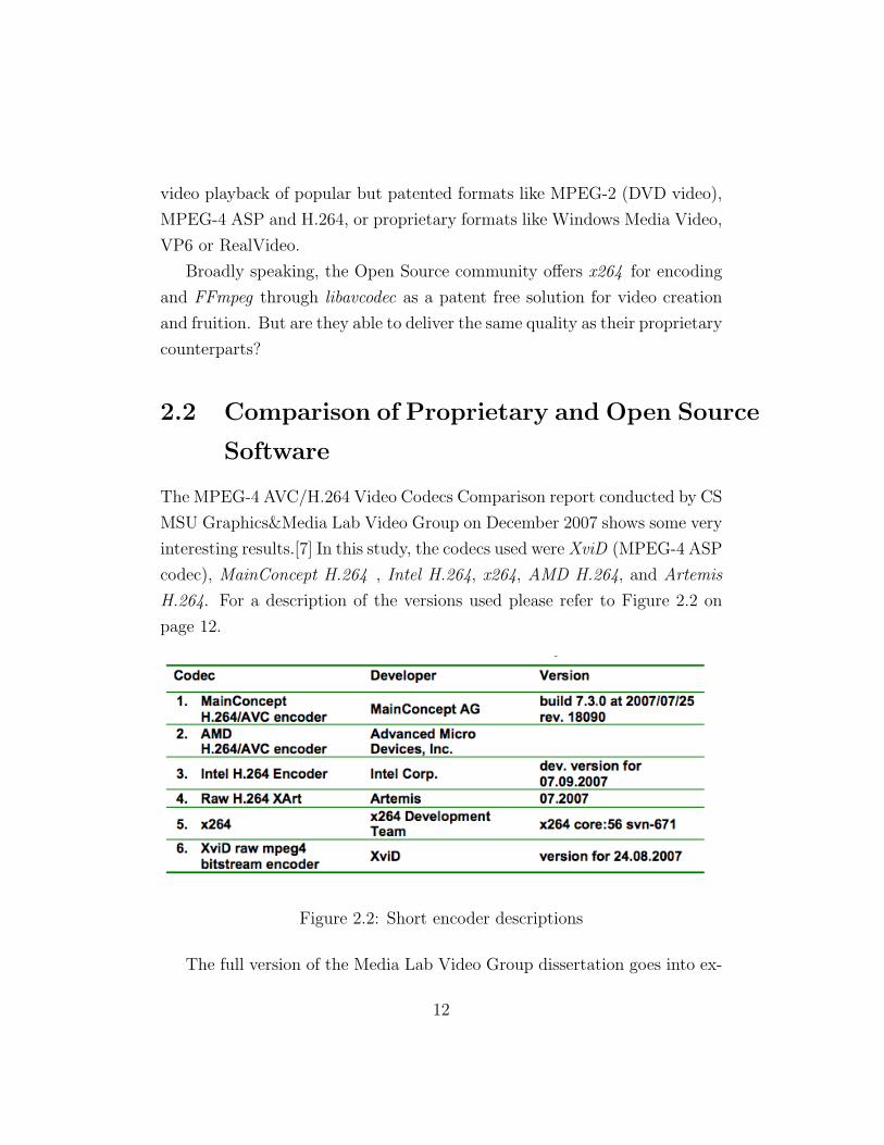
The MPEG-4 AVC/H.264 Video Codecs Comparison report conducted by CS

MSU Graphics&Media Lab Video Group on December 2007 shows some very

interesting results.[7] In this study, the codecs used were XviD (MPEG-4 ASP

codec), MainConcept H.264 , Intel H.264, x264, AMD H.264, and Artemis

H.264. For a description of the versions used please refer to Figure 2.2 on

page 12.

Figure 2.2: Short encoder descriptions

The full version of the Media Lab Video Group dissertation goes into ex-

12

tensive details, covering RD Curves, High Speed Preset, and Encoding Speed

for several Movie scenes, HDTV and video conferencing, see that for full de-

tails and explanation.[7] For the purpose of this dissertation, we will show

the Y-PSNR (see Chapter 5.1) and Y-SSIM (see Chapter 5.2) performance

comparison of the different codecs on a battle scene.

Figure 2.3: Battle scene technical details and screenshot.

Figure 2.3 is a fragment from the beginning of the Terminator 2 movie.

In terms of compression, this sequence is the most difficult among all of

the sequences that were used in the analysis. This difficulty is due to three

main reasons: continual brightness variation (resulting from explosions and

laser flashes as seen in the picture above), very fast motion and frequent

scene changes. These characteristics often cause codecs to compress frames

as I-frames.

The speed/quality trade-off graphs simultaneously show relative quality

and encoding speed for the encoders tested in this comparison. XviD is the

13

Figure 2.4: Speed/Quality tradeoff. Usage area Movies, Battle sequence,High Quality preset, Y-PSNR.

reference codec with both quality and speed normalized to unity for all of

the below graphs. The terms better and worse are used to compare codecs

in the same manner as in previous portions of this comparison.

Figure 2.4 shows examples of the results for the High Quality preset.

MainConcept and x264 are the clear leaders, the former being faster, the

latter producing better quality images. Since the Y-PSNR and Y-SSIM re-

sults are very similar, only one graph is shown.

Overall, the leaders in this comparison are the MainConcept and the x264

encoders, with the Intel IPP encoder taking a strong third place (Figure 2.4

and 2.5). The XviD (MPEG-4 ASP) codec is, on average, better than the

14

Figure 2.5: Average bitrate ratio for a fixed quality for all categories and allpresets (Y-SSIM).

AMD and Artemis x264 codecs, which proves that the AMD and Artemis

x264 encoders did not use all of the features of the H.264 standard. The

XviD codec demonstrates difficulties with bitrate handling algorithms, so

does the AMD encoder as well.

The overall ranking of the codecs tested in this comparison is as follows:

1. MainConcept

2. x264

3. Intel IPP

4. XviD

5. Artemis x264

6. AMD

This rank based only on quality results of encoders, meaning that en-

coding speed is not considered. The difference between the MainConcept

15

and x264 encoders is not overly significant, so these two encoders are both

the clear leaders in this comparison. The developers of the Artemis x264

encoder do not provide a High Quality preset, so its ranking is based solely

on the results for the High Speed preset. The quality of the Artemis x264

(H.264) codec is lower than that of XviD (MPEG-4 ASP), which means that

the developers of Artemis x264 did not employ the x264 encoder, which they

modified, to its fullest potential. The low quality of AMD could be explained

by its high encoding speed; the developers of the AMD codec did not provide

a slow preset for use in this comparison, so tests of the AMD codec only used

a very fast preset (5 to 10 times faster than that of its competitors).[7]

The conclusions of these tests are quite promising for the Open Source

community. x264 shows no significant difference from the best commercial

encoder. It comes as no surprise that even companies implemented a technol-

ogy based on this OSS codec for their commercial projects, such as Google

Video, MobileASL, Speed Demos Archive, and TASvideos.7

Furthermore, as of August 2009, x264 implements more features than any

other H.264 encoder. (See Figure 2.6, Software encoder feature comparison

on page 18.)

The problem with H.264 is that it’s not free. In countries where patents

on software algorithms are upheld, the vendors of products which make use

of H.264/AVC are expected to pay patent licensing royalties for the patented

technology that their products use. This applies to the Baseline Profile as

well.8 A private organisation known as MPEG LA, which is not affiliated

in any way with the MPEG standardisation organisation, administers the

licenses for patents applying to this standard, as well as the patent pools for

MPEG-2 Part 1 Systems, MPEG-2 Part 2 Video, MPEG-4 Part 2 Video,

and other technologies.

The problems are not just within the realm of software development - if

7http://www.videolan.org/developers/x264.html8http://blogs.sun.com/openmediacommons/entry/oms_video_a_project_of

16

one creates or publishes video online then patent-encumbered technologies

affect them directly. Patent holders have the power to extract fees from con-

tent producers and MPEG LA, which represents patent holders of the popular

MPEG video technologies, charges license fees from television broadcasters,

DVD distributors, and others. At this moment they don’t charge for online

distribution, but at the end of 2009 they are expected to announce new roy-

alty terms, and these new terms could threaten independent publishers of

online video.

While x264 offers an excellent implementation of the H.264 specifics and

may solve the technical solution to Open Source lossy video encoder, it does

not ensure that the world will be able to freely use this technology in the

future, as the patent stranglehold is still limiting its usage. A growing need

for a free-as-in-beer video codec has given the light to interesting projects,

the most notable of which is called Ogg Theora.

17

Figure 2.6: Software encoder feature comparison.18

Chapter 3

Ogg Theora

Ogg Theora is an open and royalty-free lossy video compression technology

being developed by the Xiph.Org Foundation as part of their Ogg project.

It is based on an older technology called VP3, originally a proprietary and

patented video format developed by a company called On2 Technologies. In

September 2001, On2 donated VP3 to the Xiph.Org Foundation under a free

software license. On2 also made an irrevocable, royalty-free license grant

for any patent claims it might have over the software and any derivatives,

allowing anyone to build on the VP3 technology and use it for any purpose.

In 2002, On2 entered into an agreement with the Xiph.Org Foundation to

make VP3 the basis of a new, free video format called Theora. On2 declared

Theora to be the successor to VP3.

The Xiph.Org Foundation is a non-profit organisation, that focuses on

the production and mainstreaming of free multimedia formats and software.

In addition to the development of Theora, they developed the free audio

codec Vorbis, as well as a number of very useful tools and components that

make free multimedia software easier and more comfortable to use. After

several years of beta status, Theora released its first stable (1.0) version in

November 2008. Videos encoded with any version of Theora since this point

will continue to be compatible with any future player. A broad community

19

of developers with support from companies like Redhat and NGOs like the

Wikimedia Foundation continue to improve Theora.

Because distribution and improvement of Theora is not limited by patents,

it can be included in free software. Distributions of GNU/Linux-based op-

erating systems, such as Ubuntu, Debian GNU/Linux, or Fedora, all in-

clude Theora ”out-of-the-box”, as well as modern web browsers like Firefox,

Chrome, and Opera also support Theora. If we consider the six major us-

age share of web browsers statistics of July 2009, approximately 31.28% of

Internet users across all of these statistics are using Mozilla Firefox, 3.23%

are using Google Chrome and 1.19% Opera as their browser, all of which

are growing especially Firefox.1 This means that every day a huge number

of people are using software capable of playing Theora video, approximately

36% of all internet users, or 605 million.2

Theora is a lossy video compression method. The compressed video can

be stored in any suitable container format. Theora video is generally included

in Ogg container format and is frequently paired with Vorbis format audio

streams.

The combination of the Ogg container format, Theora-encoded video, and

Vorbis-encoded audio allows for a completely open, royalty-free multimedia

format. We’ve covered before the fact that other multimedia formats, such

as MPEG-4 video and MP3 audio, are patented and subject to license fees

for commercial use. Like many other image and video formats, Theora uses

chroma subsampling, block based motion compensation and an 8 by 8 DCT

block, which makes it comparable to MPEG-1/2/4. It also supports intra

coded frames and forward predictive frames but not bi-predictive frames that

can be found in many other video codecs.[5]

As a new format with little commercial support, Theora is struggling to

gain acceptance from distributors, especially on the web. On the other hand,

1W3Counter http://w3counter.com/globalstats.php2INTERNET USAGE STATISTICS, The Internet Big Picture, World Internet Users

and Population Stats http://www.internetworldstats.com/stats.htm

20

as the only mature royalty free video codec (as of August 2009), it is well

established both as a baseline video format in modern free software and as

the format of choice for Wikipedia and many other organisations, such as

DailyMotion and The Video Bay.

3.1 Technical specification

Features available in the Theora format (and a comparison to VP3 and

MPEG-4 ASP):

• 8x8 Type-II Discrete Cosine Transform

• block-based motion compensation

• free-form variable bit rates (VBR)

• adaptive in-loop deblocking applied to the edges of the coded blocks

(not existing in MPEG-4 ASP)

• block sizes down to 8x8 (MPEG-4 ASP supports 8x8 only with 4MV)

• 384 8x8 custom quantization matrices: intra/inter, luma/chroma and

even each quant (more than VP3 and MPEG-4 ASP/AVC)

• flexible entropy encoding (Theora supports 80 VLC tables selectable

per-frame, MPEG-4 ASP has just one)

• 4:2:0, 4:2:2, and 4:4:4 chroma subsampling formats (VP3 and MPEG-4

ASP only support 4:2:0)

• 8 bits per pixel per colour channel

• multiple reference frames (not possible in MPEG-4 ASP)

• pixel aspect ratio (eg for anamorphic signalling/playback)

21

• non-multiple of 16 picture sizes (as possible in ASP, but not in VP3)

• non-linear scaling of quants values (as done in MPEG-4 AVC)

• adaptive quantization down to the block level (as possible in MPEG-4

ASP/AVC, but not in VP3)

• intra frames (I-Frames in MPEG), inter frames (P-Frames), but no

B-Frames (as supported in MPEG-4 ASP/AVC)

• HalfPixel Motion Search Precision (MPEG-4 ASP/AVC supports Half-

Pixel or QuarterPixel)

• technologies used already in Vorbis (decoder setup configuration, bit-

stream headers...) not available in VP3

3.2 Theora and the Web

Support for Theora video in browsers creates a special opportunity. Right

now, nearly all online video requires Flash, a product owned by one com-

pany. But, now that around 36% of users can play Theora videos in their

browser without having to install additional software, it is possible to chal-

lenge Flash’s dominance as a web video distribution tool. Additionally, the

new HTML5 standard by the W3C (World Wide Web Consortium) adds an-

other exciting dimension: an integration of the web and video in new and

exciting ways that complement Theora.

3.3 Ogg Theora vs. x264

On May 7, 2009, it was reported that ”Xiph hackers have been hard at work

improving the Theora codec over the past year, with the latest versions gain-

ing on and passing h.264 in objective PSNR quality measurements.3” As it

3http://tech.slashdot.org/article.pl?sid=09/05/07/2352203&tid=188

22

turns out, there was an error in the methadology used in the original com-

parison, which hit x264 for more than 4 dB of difference.4 Nevertheless, the

growing interest in the need for Open Video codecs, the wide acceptance by

large video providers and the recent improvements of the video codec sug-

gest that the argument is far from being well defined as a loss of the Open

Source community. We know very well that the PSNR comparison is not

particularly reliable when it comes to perceived quality, which is what we

are most interested in. Other comparisons have taken place, and they sug-

gest that the perceivable difference at relatively low, web-like bitrates, is not

especially great.5

Let us consider Greg Maxwell’s work in this regard.

3.4 Ogg Theora - YouTube subjective com-

parison

In order to avoid any possible bias in the selection of H.264 encoders and

encoding options, and to maximize the relevance for this particular issue, it

was used YouTube itself as the H.264 encoder. This is less than ideal because

YouTube does not accept lossless input, but it does accept arbitrarily high

bitrate inputs.

The footage comes from the Blender Foundation’s Big Buck Bunny as

test case because of its clear licensing status, because it’s a real world test

case, and because it is available in a lossless native format. The choice of

the footage and the methodology used are probably not the most efficient

for either Theora or H.264, but it serves the purpose of this dissertation: we

4They used ffmpeg for outputting the raw y4m file to have its quality measuredby dump psnr (but not for theora). Apparently, ffmpeg flags the output chroma as”420mpeg2” instead of ”420”, which results in over 4db of PSNR being slashed offof x264’s results unfairly. http://www.reddit.com/r/programming/comments/8iphn/theora_encoder_improvments_comparable_to_h264/c09eyvc.

5urlhttp://people.xiph.org/ greg/video/ytcompare/comparison.html

23

want to consider a real world situation in a web environment: YouTube may

not produce the best H.264 output, but it’s the most commonly used and

therefore it represents what people will actually see, not what they should

ideally see.

This particular test case has also a soundtrack, because most real usage

has sound. No one implements HTML5 video without audio, and no one is

implementing either of Theora or Vorbis without the other. Vorbis’s state-

of-the-art performance is a contributor to the overall Ogg/Theora+Vorbis

solution.

3.4.1 Methodology

The following steps were followed to produce the comparison:

1. Obtain the lossless 640x360 Big Buck Bunny source PNGs and FLACs

from http://media.xiph.org.

2. Resample the images to 480x270 using ImageMagick’s convert utility.

3. Use gstreamer’s jpegenc, produce a quality = 100mjpeg + PCM au-

dio stream. The result is around 1.5Gbytes with a bitrate of around

20Mbit/sec.

4. Truncate the file to fit under the YouTube 1Gbyte limit, resulting in

inputmjpeg.avi(706MiB).

5. Upload the file to YouTube and wait for it to transcode.

6. Download the FLV and H.264 files produced by YouTube using one of

the many web downloading services.

7. Using libtheora 1.1a2 and Vorbis aoTuv 5.7 produce a file of compara-

ble bitrate to the youtube 499kbit/sec from the same file uploaded to

YouTube (input mjpeg.avi).

24

8. Resample the file uploaded to YouTube to 400x226.

9. Using libtheora 1.1a2 and Vorbis aoTuv 5.7 produce a file of comparable

bitrate to the youtube 327kbit/sec from the 400x226 downsampled copy

of input mjpeg.avi.

A keyframe interval of 250 frames was used for the Theora encoding. The

theora 1.1a2 encoder software used is available from http://theora.org.

The Vorbis encoder used is available from the aoTuV website. No software

modifications were performed.

A 499kbit/secH.264 + AAC output and a 327kbit/sec H.263(Sorensen

Spark)+MP3 output were available via the download service. The YouTube-

encoded files are available on the YouTube site. Because the files on YouTube

may change and the web player does not disclose the underlying bitrate, the

two encoded files were available to download from the Maxwell’s website.

3.4.2 Results

It can be difficult to compare video at low bitrates, and even YouTube’s

higher bitrate option is not high enough to achieve good quality. The primary

challenge is that all files at these rates will have problems, so the reviewer is

often forced to decide which of two entirely distinct flaws is worse.

Maxwell’s conclusion is that Theora + V orbis results are substantially

better than the YouTube 327kbit/sec. This is unsurprising since the Xiph

team’s position has long been that Theora is better than H.263, especially

at lower bitrates, and YouTube only uses a subset of H.263.(Figures 3.1 and

3.2)

The low bitrate case is also helped by Vorbis’ considerable superiority

over MP3. For example, at the beginning of the clip there are crickets

singings, which are inaudible in the low rate YouTube clip but sound fine

in the Ogg/Theora+Vorbis version.

25

Figure 3.1: Frame 366: Ogg/Theora+Vorbis 325kbit/sec overall.

Figure 3.2: Frame 366: YouTube 2009-06-13 327kbit/sec overall.

26

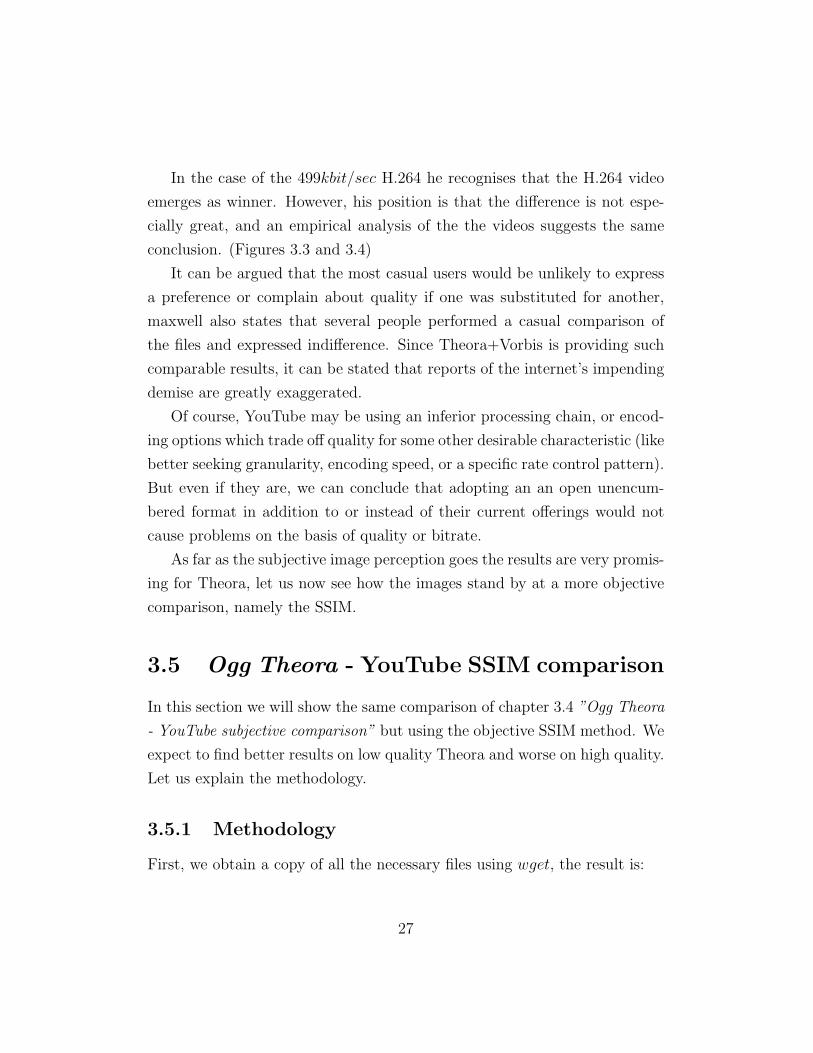
In the case of the 499kbit/sec H.264 he recognises that the H.264 video

emerges as winner. However, his position is that the difference is not espe-

cially great, and an empirical analysis of the the videos suggests the same

conclusion. (Figures 3.3 and 3.4)

It can be argued that the most casual users would be unlikely to express

a preference or complain about quality if one was substituted for another,

maxwell also states that several people performed a casual comparison of

the files and expressed indifference. Since Theora+Vorbis is providing such

comparable results, it can be stated that reports of the internet’s impending

demise are greatly exaggerated.

Of course, YouTube may be using an inferior processing chain, or encod-

ing options which trade off quality for some other desirable characteristic (like

better seeking granularity, encoding speed, or a specific rate control pattern).

But even if they are, we can conclude that adopting an an open unencum-

bered format in addition to or instead of their current offerings would not

cause problems on the basis of quality or bitrate.

As far as the subjective image perception goes the results are very promis-

ing for Theora, let us now see how the images stand by at a more objective

comparison, namely the SSIM.

3.5 Ogg Theora - YouTube SSIM comparison

In this section we will show the same comparison of chapter 3.4 ”Ogg Theora

- YouTube subjective comparison” but using the objective SSIM method. We

expect to find better results on low quality Theora and worse on high quality.

Let us explain the methodology.

3.5.1 Methodology

First, we obtain a copy of all the necessary files using wget, the result is:

27

11M bbb_theora_325kbit.ogv

11M bbb_youtube_lowquality_327kbit.flv

17M bbb_theora_486kbit.ogv

17M bbb_youtube_h264_499kbit.mp4

580M input_mjpeg.avi

Where:

• bbb theora 325kbit.ogv is the low quality Theora file at 325kbit/s.

• bbb youtube lowquality 327kbit.f lv is the low quality FLV file at 327kbit/s.

• bbb theora 486kbit.ogv is the high quality Theora file at 486kbit/s.

• bbb youtube h264 499kbit.mp4 is the high quality H.264 file at 499kbit/s.

• input mjpeg.avi is the source input file at 17, 569.6kbit/s.

Next, we need to extract a few screenshots form each of the files, pair and

rename them properly. MPlayer6 will serve this purpose:

mplayer -vo png -frames 50 -ss 10 input_mjpeg.avi

mplayer -vo png -frames 50 -ss 10 bbb_theora_325kbit.ogv

mplayer -vo png -frames 50 -ss 10 bbb_youtube_lowquality_327kbit.flv

mplayer -vo png -frames 50 -ss 10 bbb_theora_486kbit.ogv

mplayer -vo png -frames 50 -ss 10 bbb_youtube_h264_499kbit.mp4

6MPlayer is a free and open source media player. The program is available for allmajor operating systems, including Linux and other Unix-like systems, Microsoft Win-dows and Mac OS X. Versions for OS/2, Syllable, AmigaOS and MorphOS are alsoavailable. The Windows version works, with some minor problems, also in DOS usingHX DOS Extender. A port for DOS using DJGPP is also available. A version for theWii Homebrew Channel has also emerged. It plays most MPEG/VOB, AVI, Ogg/OGM,VIVO, ASF/WMA/WMV, QT/MOV/MP4, RealMedia, Matroska, NUT, NuppelVideo,FLI, YUV4MPEG, FILM, RoQ, PVA files, supported by many native, XAnim, andWin32 DLL codecs. You can watch VideoCD, SVCD, DVD, 3ivx, DivX 3/4/5, WMVand even H.264 movies. Version used: MPlayer dev-SVN-r27807-4.0.1. Available at:svn://svn.mplayerhq.hu/mplayer/trunkmplayer

28

This will extract 50 consecutive frames on lossless PNG format starting

from the 10th second. We will then chose a few significant images.

In this example we chose two particular frames: the screenshot in Figure

3.5 represents a static image with a relatively simple scenery, while Figure

3.6 is the beginning of an action sequence, the ripples on the water are very

hard to encode and usually require a high quality compression.

Now, we use ImageJ7 to compare the same frames taken from low quality

Theora and the FLV.

The same argument applies for the second frame.

Let us now see the SSIM comparison results.

7ImageJ is a public domain Java image processing program inspired by NIH Image forthe Macintosh. It runs, either as an online applet or as a downloadable application, onany computer with a Java 1.4 or later virtual machine. Downloadable distributions areavailable for Windows, Mac OS, Mac OS X and Linux. Version used: 1.42q Available at:http://rsbweb.nih.gov/ij/

29

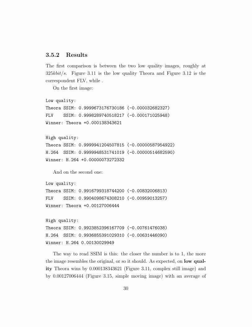
3.5.2 Results

The first comparison is between the two low quality images, roughly at

325kbit/s. Figure 3.11 is the low quality Theora and Figure 3.12 is the

correspondent FLV, while .

On the first image:

Low quality:

Theora SSIM: 0.9999673176730186 (-0.000032682327)

FLV SSIM: 0.9998289740518217 (-0.000171025948)

Winner: Theora +0.000138343621

High quality:

Theora SSIM: 0.9999941204507815 (-0.00000587954922)

H.264 SSIM: 0.9999948531741019 (-0.00000514682590)

Winner: H.264 +0.00000073272332

And on the second one:

Low quality:

Theora SSIM: 0.9916799318744200 (-0.00832006813)

FLV SSIM: 0.9904098674308210 (-0.00959013257)

Winner: Theora +0.00127006444

High quality:

Theora SSIM: 0.9923852396167709 (-0.00761476038)

H.264 SSIM: 0.9936855391029310 (-0.00631446090)

Winner: H.264 0.00130029949

The way to read SSIM is this: the closer the number is to 1, the more

the image resembles the original, or so it should. As expected, on low qual-

ity Theora wins by 0.000138343621 (Figure 3.11, complex still image) and

by 0.00127006444 (Figure 3.15, simple moving image) with an average of

30

0.000704204031. On high quality H.264 wins by 0.00000073272332 (Figure

3.14) and by 0.00130029949 (Figure 3.18) with an average of 0.000650516107.

Overall, the SSIM comparison confirms the subjective analysis. However,

there are several fallacies with this method of analysis:

• low quality images had to be upscaled in order to fit the minimum 256

pixel required for the comparison

• all images had to be converted to grayscale

• in order to have a statistically significant result all frames should be

analysed, not just a very small portion. Unfortunately this is not an

easy task, as the Java program we used for this purpose is not script-

able, and the MSU Video Quality Measurement Tool PRO Version,

capable of such a task, is a commercial application costing 724e.

Given this consideration, the results are in line with our predictions and

they confirm what we already observed though a subjective analysis.

31

Figure 3.3: Frame 366: Ogg/Theora+Vorbis 486kbit/sec overall.

32

Figure 3.4: Frame 366: YouTube 2009-06-13 499kbit/sec overall.

Figure 3.5: First frame: PNG from the source input file at 17, 569.6kbit/s.

33

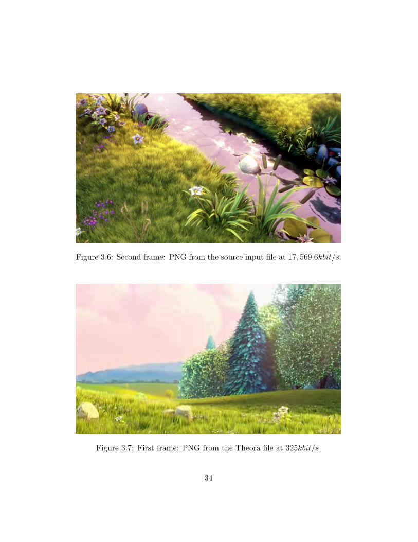
Figure 3.6: Second frame: PNG from the source input file at 17, 569.6kbit/s.

Figure 3.7: First frame: PNG from the Theora file at 325kbit/s.

34

Figure 3.8: First frame: PNG from the FLV file at 327kbit/s.

Figure 3.9: First frame: PNG from the Theora file at 486kbit/s.

35

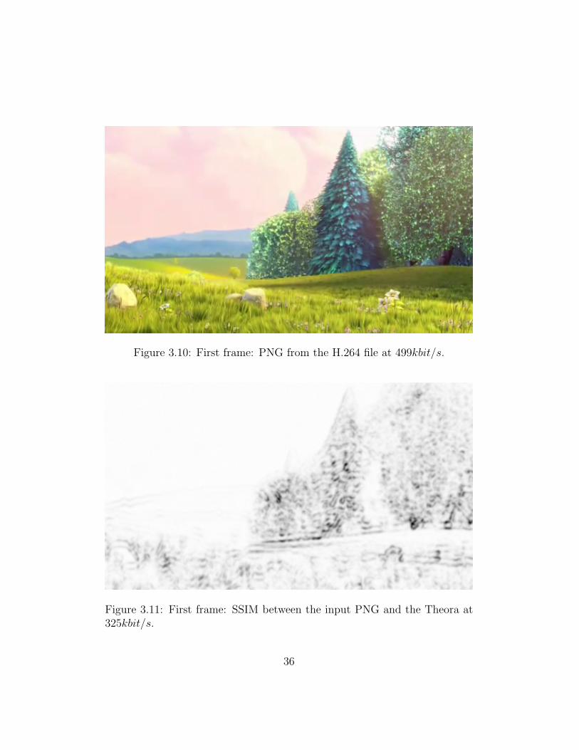
Figure 3.10: First frame: PNG from the H.264 file at 499kbit/s.

Figure 3.11: First frame: SSIM between the input PNG and the Theora at325kbit/s.

36

Figure 3.12: First frame: SSIM between the input PNG and the FLV at327kbit/s.

Figure 3.13: First frame: SSIM between the input PNG and the Theora at486kbit/s.

37

Figure 3.14: First frame: SSIM between the input PNG and the H.264 at499kbit/s.

Figure 3.15: Second frame: SSIM between the input PNG and the Theoraat 325kbit/s.

38

Figure 3.16: Second frame: SSIM between the input PNG and the FLV at327kbit/s.

Figure 3.17: Second frame: SSIM between the input PNG and the Theoraat 486kbit/s.

39

Figure 3.18: Second frame: SSIM between the input PNG and the H.264 at499kbit/s.

40

Chapter 4

Conclusions

We have explored the technical capabilities of the latest lossy video compres-

sion technologies which could be applied for Web distribution, be it either

though Web browsers of handheld devices. Ogg Theora, after a subjective

as well as an objective analysis, seems to offers a viable solution for video

distribution without compromising the video quality. Given that Theora is

fully supported by HTML5, it’s an open standard free of commercial limita-

tions and patents, and that some of the most visited websites of the world

are already supporting it as well as most of the browsers, there seems to be

no reason for not supporting it.

However, when we look at the market we see, as often happens, that

best technical solution is not the preferred one. Apple, with the iPhone and

the various versions of iPod, has almost has the monopoly of portable video

player, and has already stated that they are not going to support it. Nokia,

the number one provider of cellphones, follows the same path.

Also, no matter what everyone else does, Internet Explorer still has the

largest user base, and has no intention of supporting Theora, nor HTML5

for that matter, and this is a fact that we cannot ignore. Ryan Paul of

Arctechnica suggests that: ”It’s unfortunate that this debate is threatening to

derail the adoption of standards-based Internet video solutions. The dominant

41

video solution today is Flash, a proprietary technology that is controlled by

a single vendor and doesn’t perform well on Linux or Mac OS X. There is

a clear need for an open alternative, but the codec controversy could make it

difficult.”. He then cleverly adds: ”My inner pessimist suspects that Microsoft

will finally get around to implementing HTML5 video at the same time that

the H.264 patents expire, in roughly 2025 ”.

What sense does it make to have a standard, if not everyone agrees and

uses it? We can only hope that this technological madness will eventually

stop, and that reason will prevail.

I have hope for the future of video distribution and the internet. In fact,

just a few days ago, after much of this dissertation wa written, in a recent

message that has come as a shock to many, Microsoft endorsed the use of

< video > and < audio > tags, as reported by Adrian Bateman, the Program

Manager for Internet Explorer in the W3 mailing list1, even though they are

still discussing the details. There is hope indeed, the technological future

might brighter than we think.

1We support the inclusion of the < video > and < audio > elements in the spec. Thereare a couple of areas that we have some thoughts - we are still discussing the details[...]Adrian. http://lists.w3.org/Archives/Public/public-html/2009Sep/0049.html

42

Chapter 5

Appendix: Objective Quality

Metrics Description

In this chapter I shall present the Objective Quality Metrics Descrip-

tion, algorithms used in this dissertation to determine which video encoder

shows the best results, Peak Signal-to-Noise Ratio (PSNR) and Structural

SIMilarity (SSIM).

5.1 Peak Signal-to-Noise Ratio

The phrase peak signal-to-noise ratio, often abbreviated PSNR, is an engi-

neering term for the ratio between the maximum possible power of a signal

and the power of corrupting noise that affects the fidelity of its representa-

tion. Because many signals have a very wide dynamic range, PSNR is usually

expressed in terms of the logarithmic decibel scale.

The PSNR is most commonly used as a measure of quality of reconstruc-

tion of lossy compression codecs (e.g. for image compression). The signal in

this case is the original data, and the noise is the error introduced by com-

pression. When comparing compression codecs it is used as an approximation

to human perception of reconstruction quality, therefore in some cases one

43

reconstruction may appear to be closer to the original than another, even

though it has a lower PSNR (a higher PSNR would normally indicate that

the reconstruction is of higher quality).

It is most easily defined via the mean squared error (MSE) which for two

m× n monochrome images I and K where one of the images is considered a

noisy approximation of the other is defined as:

MSE =1

mn

m−1∑i=0

n−1∑j=0

||I(i, j)−K(i, j)||2

The PSNR is defined as:

PSNR = 10 · log10

(MAX 2

I

MSE

)= 20 · log10

(MAX I√

MSE

)Here, MAXi is the maximum possible pixel value of the image. When the

pixels are represented using 8 bits per sample, this is 255. More generally,

when samples are represented using linear PCM with B bits per sample,

MAXI is 2B − 1. For colour images with three RGB values per pixel, the

definition of PSNR is the same except the MSE is the sum over all squared

value differences divided by image size and by three.

Typical values for the PSNR in lossy image and video compression are

between 30 and 50 dB, where higher is better.1 Acceptable values for wireless

transmission quality loss are considered to be about 20 dB to 25 dB.2 When

the two images are identical the MSE will be equal to zero, resulting in an

infinite PSNR.

In particular, the formula used for all the benchmark in Chapter 2 Ad-

1Thomos, N., Boulgouris, N. V., & Strintzis, M. G. (2006, January). Optimized Trans-mission of JPEG2000 Streams Over Wireless Channels. IEEE Transactions on ImageProcessing , 15 (1)

2Xiangjun, L., & Jianfei, C. ROBUST TRANSMISSION OF JPEG2000 ENCODEDIMAGES OVER PACKET LOSS CHANNELS. ICME 2007 (pp. 947-950). School ofComputer Engineering, Nanyang Technological University.

vanced Video Coding and OSS is the following:

d(X, Y ) = 10 · log102552m · n∑m,n

i=1,j=1(xij − yij)2

Where:

• d(X, Y ) — PSNR value between X and Y frames

• xij — the pixel value for (i, j) position for the X frame

• yij — the pixel value for (i, j) position for the Y frame

• m,n — frame size mxn

Generally, this metric has the same form as the mean square error (MSE),

but it is more convenient to use because of the logarithmic scale. It still has

the same disadvantages as the MSE metric, however.

In MSU Video Quality Measurement Tool the PSNR can be calculated

for all YUV and RGB components and for the L component of LUV colour

space. The PSNR value is quick and easy to calculate, but it is sometimes

inappropriate as relates to human visual perception.

A maximum deviation of 255 is used for the PSNR for the RGB and

YUV colour components because, in YUV files, there is 1 byte for each

colour component. The maximum possible difference, therefore, is 255. For

the LUV colour space, the maximum deviation is 100.

The values of the PSNR in the LUV colour space are in the range [0,

100]; the value 100 means that the frames are identical.

5.1.1 PSNR Examples

PSNR visualization uses different colours for better visual representation:

• Black — value is very small (99–100)

• Blue — value is small (35–99)

• Green — value is moderate (20–35)

• Yellow — value is high (17–20)

• Red — value is very high (0–17)

Figure 5.1 is an example of the PSNR metric for two frames.

Figure 5.1: PSNR example for two frames.

Figures 5.2 and 5.3 are further examples demonstrating how various dis-

tortions can influence the PSNR value. Figure 5.2 represents three distortions

of the original image (top-left) and their relative PSNR value in Figure 5.3.

Figure 5.2: Original and processed images (for PSNR example).

5.2 Structural SIMilarity

The Structural SIMilarity (SSIM) index is a method for measuring the simi-

larity between two images. The SSIM index is a full reference metric, in other

words, the measuring of image quality based on an initial uncompressed or

distortion-free image as reference. SSIM is designed to improve on tradi-

tional methods like PSNR and MSE, which have proved to be inconsistent

with human eye perception.

The SSIM metric is calculated on various windows of an image. The

measure between two windows of size NxN x and y is :

SSIM(x, y) =(2µxµy + c1)(2covxy + c2)

(µ2x + µ2

y + c1)(σ2x + σ2

y + c2)

with:

• µx the average of x

• µy the average of y

• σ2x the variance of x

• σ2y the variance of y

• covxy the covariance of y

• c1 = (k1L)2, c2 = (k2L)2 two variables to stabilize the division with

weak denominator

• L the dynamic range of the pixel-values (typically this is 2#bits per pixel−1)

• k1 = 0.01 and k2 = 0.03 by default.

For the implementation used in this comparison, one SSIM value corre-

sponds to two sequences. The value is in the range [-1, 1], with higher values

being more desirable (a value of 1 corresponds to identical frames). One of

the advantages of the SSIM metric is that it better represents human visual

perception than does PSNR. SSIM is more complex, however, and takes more

time to calculate.

5.2.1 SSIM Examples

Figure 5.4 is an example of an SSIM result for an original and processed

(compressed with lossy compression) image. The closer the SSIM is to 1, the

more the processed image resembles the original. The resulting value of 0.9

demonstrates that the two images are fairly similar.

Figures 5.5 and 5.6 who the same comparison as we did with the PSNR

value in chapter 5.1.1.

Figure 5.3: PSNR values for original and processed images.

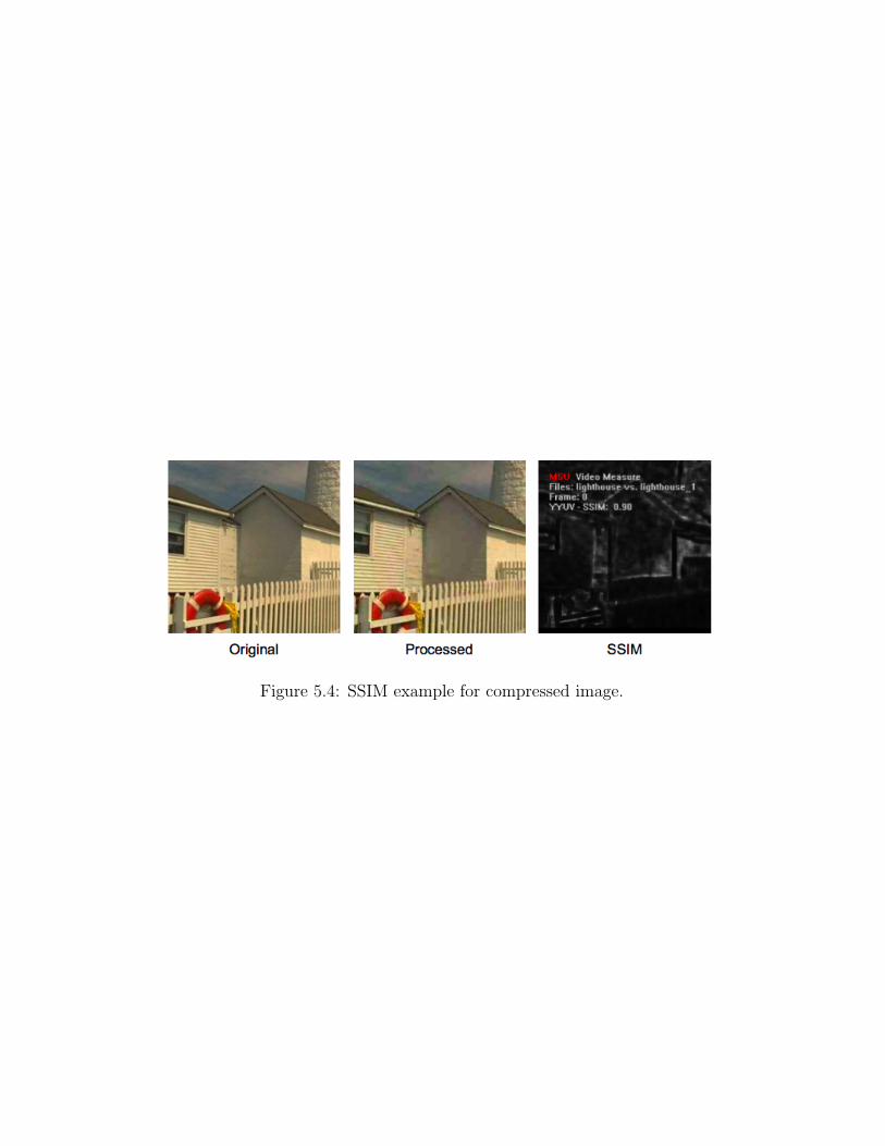
Figure 5.4: SSIM example for compressed image.

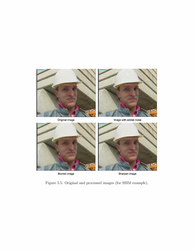
Figure 5.5: Original and processed images (for SSIM example).

Figure 5.6: SSIM values for original and processed images.

List of Figures

2.1 Worldwide Ubiquity of Adobe Flash Player by Version - March

2009. . . . . . . . . . . . . . . . . . . . . . . . . . . . . . . . . 11

2.2 Short encoder descriptions . . . . . . . . . . . . . . . . . . . . 12

2.3 Battle scene technical details and screenshot. . . . . . . . . . . 13

2.4 Speed/Quality tradeoff. Usage area Movies, Battle sequence,

High Quality preset, Y-PSNR. . . . . . . . . . . . . . . . . . . 14

2.5 Average bitrate ratio for a fixed quality for all categories and

all presets (Y-SSIM). . . . . . . . . . . . . . . . . . . . . . . . 15

2.6 Software encoder feature comparison. . . . . . . . . . . . . . . 18

3.1 Frame 366: Ogg/Theora+Vorbis 325kbit/sec overall. . . . . . 26

3.2 Frame 366: YouTube 2009-06-13 327kbit/sec overall. . . . . . 26

3.3 Frame 366: Ogg/Theora+Vorbis 486kbit/sec overall. . . . . . 32

3.4 Frame 366: YouTube 2009-06-13 499kbit/sec overall. . . . . . 33

3.5 First frame: PNG from the source input file at 17, 569.6kbit/s. 33

3.6 Second frame: PNG from the source input file at 17, 569.6kbit/s. 34

3.7 First frame: PNG from the Theora file at 325kbit/s. . . . . . . 34

3.8 First frame: PNG from the FLV file at 327kbit/s. . . . . . . . 35

3.9 First frame: PNG from the Theora file at 486kbit/s. . . . . . . 35

3.10 First frame: PNG from the H.264 file at 499kbit/s. . . . . . . 36

3.11 First frame: SSIM between the input PNG and the Theora at

325kbit/s. . . . . . . . . . . . . . . . . . . . . . . . . . . . . . 36

54

3.12 First frame: SSIM between the input PNG and the FLV at

327kbit/s. . . . . . . . . . . . . . . . . . . . . . . . . . . . . . 37

3.13 First frame: SSIM between the input PNG and the Theora at

486kbit/s. . . . . . . . . . . . . . . . . . . . . . . . . . . . . . 37

3.14 First frame: SSIM between the input PNG and the H.264 at

499kbit/s. . . . . . . . . . . . . . . . . . . . . . . . . . . . . . 38

3.15 Second frame: SSIM between the input PNG and the Theora

at 325kbit/s. . . . . . . . . . . . . . . . . . . . . . . . . . . . . 38

3.16 Second frame: SSIM between the input PNG and the FLV at

327kbit/s. . . . . . . . . . . . . . . . . . . . . . . . . . . . . . 39

3.17 Second frame: SSIM between the input PNG and the Theora

at 486kbit/s. . . . . . . . . . . . . . . . . . . . . . . . . . . . . 39

3.18 Second frame: SSIM between the input PNG and the H.264

at 499kbit/s. . . . . . . . . . . . . . . . . . . . . . . . . . . . . 40

5.1 PSNR example for two frames. . . . . . . . . . . . . . . . . . . 46

5.2 Original and processed images (for PSNR example). . . . . . . 47

5.3 PSNR values for original and processed images. . . . . . . . . 50

5.4 SSIM example for compressed image. . . . . . . . . . . . . . . 51

5.5 Original and processed images (for SSIM example). . . . . . . 52

5.6 SSIM values for original and processed images. . . . . . . . . . 53

Bibliography

[1] Jan Gerber Homes Wilson, Susanne Lang, David Khling, Jrn Seger,

Theora Cookbook, August 10-15, 2009, available at: http://en.

flossmanuals.net/TheoraCookbook/

[2] Detlev Marpe, Member, IEEE, Heiko Schwarz, Thomas Wiegand

Context-Based Adaptive Binary Arithmetic Coding in the H.264/AVC

Video Compression Standard, IEEE TRANSACTIONS ON CIRCUITS

AND SYSTEMS FOR VIDEO TECHNOLOGY, VOL. 13, NO. 7, JULY

2003

[3] Sebastian Moeritz, Klaus Diepold, Understanding MPEG 4: Technology

and Business Insights, Focal Press, September 28, 2004, p.78

[4] Wes Simpson, Video Over IP, Second Edition: IPTV, Internet Video,

H.264, P2P, Web TV, and Streaming: A Complete Guide to Understand-

ing the Technology, Focal Press Media Technology Professional Series,

[5] Xiph.org Foundation, Theora Specication, November 3, 2008, available

at: http://theora.org/doc/Theora_I_spec.pdf

[6] Zhou Wang, Alan Conrad Bovik, Hamid Rahim Sheikh, Eero P. Simon-

celli, Image Quality Assessment: From Error Visibility to Structural Sim-

ilarity, IEEE Transactions on Image Processing, Vol. 13, No. 4, April

2004.

56

[7] Dmitriy Vatolin Dmitriy Kulikov, Alexander Parshin, MPEG-4

AVC/H.264 Video Codecs Comparison, Amer. CS MSU Graphics Media

Lab (December 2007).

[8] John Watkinson, The MPEG Handbook, Focal Press; 1st edition Septem-

ber 2001, p.1

[9] John Watkinson, The MPEG Handbook, Focal Press; 1st edition Septem-

ber 2001, p.4

[10] John Watkinson, The MPEG Handbook, Focal Press; 1st edition Septem-

ber 2001, p. 83

[11] Thomas Wiegand, Gary J. Sullivan, Senior Member, IEEE, Gisle Bjnte-

gaard, Ajay Luthra, Senior Member, IEEE Overview of the H.264/AVC

Video Coding Standard, IEEE TRANSACTIONS ON CIRCUITS AND

SYSTEMS FOR VIDEO TECHNOLOGY, VOL. 13, NO. 7, JULY 2003.

[12] Wikipedia, Lossless data compression, September 13, 2009 snap-

shot, available at http://en.wikipedia.org/wiki/Lossless_data_

compression.

[13] Wikipedia, Moving Picture Experts Group, September 13, 2009 snap-

shot, available at http://en.wikipedia.org/wiki/Moving_Picture_

Experts_Group.

[14] Wikipedia, Video quality, September 13, 2009 snapshot, available at

http://en.wikipedia.org/wiki/Video_quality.

[15] Wikipedia, Subjective video quality, September 13, 2009 snapshot, avail-

able at http://en.wikipedia.org/wiki/Subjective_video_quality.

[16] Wikipedia, MPEG-4 AVC, September 13, 2009 snapshot, available at

http://en.wikipedia.org/wiki/H.264/MPEG-4_AVC.

[17] Cliff Wootton, A Practical Guide to Video and Audio Compression:

From Sprockets and Rasters to Macro Blocks, Focal Press, May 2005,

pp. p.665.