open foam - physics courses€¦ · printed book. we recommend this license principally for works...
TRANSCRIPT
Open∇FOAMThe Open Source CFD Toolbox
Programmer’s Guide
Version 1.59th July 2008

P-2
Copyright c© 2000, 2001, 2002, 2003, 2004, 2005, 2006, 2007, 2008 OpenCFD Limited.
Permission is granted to copy, distribute and/or modify this document under the termsof the GNU Free Documentation License, Version 1.2 published by the Free SoftwareFoundation; with no Invariant Sections, no Back-Cover Texts and one Front-Cover Text:“Available free from openfoam.org.” A copy of the license is included in the sectionentitled “GNU Free Documentation License”.
This document is distributed in the hope that it will be useful, but WITHOUT ANYWARRANTY; without even the implied warranty of MERCHANTABILITY or FITNESSFOR A PARTICULAR PURPOSE.
Typeset in LATEX.
Open∇FOAM-1.5

P-3
GNU Free Documentation License
Version 1.2, November 2002Copyright c©2000,2001,2002 Free Software Foundation, Inc.
59 Temple Place, Suite 330, Boston, MA 02111-1307 USA
Everyone is permitted to copy and distribute verbatim copies of this license document, butchanging it is not allowed.
Preamble
The purpose of this License is to make a manual, textbook, or other functional and usefuldocument “free” in the sense of freedom: to assure everyone the effective freedom to copy andredistribute it, with or without modifying it, either commercially or noncommercially. Secon-darily, this License preserves for the author and publisher a way to get credit for their work,while not being considered responsible for modifications made by others.
This License is a kind of “copyleft”, which means that derivative works of the documentmust themselves be free in the same sense. It complements the GNU General Public License,which is a copyleft license designed for free software.
We have designed this License in order to use it for manuals for free software, because freesoftware needs free documentation: a free program should come with manuals providing thesame freedoms that the software does. But this License is not limited to software manuals; itcan be used for any textual work, regardless of subject matter or whether it is published as aprinted book. We recommend this License principally for works whose purpose is instruction orreference.
1. APPLICABILITY AND DEFINITIONS
This License applies to any manual or other work, in any medium, that contains a notice placedby the copyright holder saying it can be distributed under the terms of this License. Such anotice grants a world-wide, royalty-free license, unlimited in duration, to use that work underthe conditions stated herein. The “Document”, below, refers to any such manual or work.Any member of the public is a licensee, and is addressed as “you”. You accept the license ifyou copy, modify or distribute the work in a way requiring permission under copyright law.
A “Modified Version” of the Document means any work containing the Document ora portion of it, either copied verbatim, or with modifications and/or translated into anotherlanguage.
A “Secondary Section” is a named appendix or a front-matter section of the Documentthat deals exclusively with the relationship of the publishers or authors of the Document tothe Document’s overall subject (or to related matters) and contains nothing that could falldirectly within that overall subject. (Thus, if the Document is in part a textbook of mathe-matics, a Secondary Section may not explain any mathematics.) The relationship could be amatter of historical connection with the subject or with related matters, or of legal, commercial,philosophical, ethical or political position regarding them.
The “Invariant Sections” are certain Secondary Sections whose titles are designated, asbeing those of Invariant Sections, in the notice that says that the Document is released underthis License. If a section does not fit the above definition of Secondary then it is not allowed to bedesignated as Invariant. The Document may contain zero Invariant Sections. If the Documentdoes not identify any Invariant Sections then there are none.
The “Cover Texts” are certain short passages of text that are listed, as Front-Cover Textsor Back-Cover Texts, in the notice that says that the Document is released under this License.A Front-Cover Text may be at most 5 words, and a Back-Cover Text may be at most 25 words.
A “Transparent” copy of the Document means a machine-readable copy, represented ina format whose specification is available to the general public, that is suitable for revising the
Open∇FOAM-1.5

P-4
document straightforwardly with generic text editors or (for images composed of pixels) genericpaint programs or (for drawings) some widely available drawing editor, and that is suitable forinput to text formatters or for automatic translation to a variety of formats suitable for input totext formatters. A copy made in an otherwise Transparent file format whose markup, or absenceof markup, has been arranged to thwart or discourage subsequent modification by readers is notTransparent. An image format is not Transparent if used for any substantial amount of text. Acopy that is not “Transparent” is called “Opaque”.
Examples of suitable formats for Transparent copies include plain ASCII without markup,Texinfo input format, LaTeX input format, SGML or XML using a publicly available DTD,and standard-conforming simple HTML, PostScript or PDF designed for human modification.Examples of transparent image formats include PNG, XCF and JPG. Opaque formats includeproprietary formats that can be read and edited only by proprietary word processors, SGML orXML for which the DTD and/or processing tools are not generally available, and the machine-generated HTML, PostScript or PDF produced by some word processors for output purposesonly.
The “Title Page” means, for a printed book, the title page itself, plus such following pagesas are needed to hold, legibly, the material this License requires to appear in the title page. Forworks in formats which do not have any title page as such, “Title Page” means the text nearthe most prominent appearance of the work’s title, preceding the beginning of the body of thetext.
A section “Entitled XYZ” means a named subunit of the Document whose title either isprecisely XYZ or contains XYZ in parentheses following text that translates XYZ in anotherlanguage. (Here XYZ stands for a specific section name mentioned below, such as “Acknowl-
edgements”, “Dedications”, “Endorsements”, or “History”.) To “Preserve the Ti-
tle” of such a section when you modify the Document means that it remains a section “EntitledXYZ” according to this definition.
The Document may include Warranty Disclaimers next to the notice which states that thisLicense applies to the Document. These Warranty Disclaimers are considered to be included byreference in this License, but only as regards disclaiming warranties: any other implication thatthese Warranty Disclaimers may have is void and has no effect on the meaning of this License.
2. VERBATIM COPYING
You may copy and distribute the Document in any medium, either commercially or noncom-mercially, provided that this License, the copyright notices, and the license notice saying thisLicense applies to the Document are reproduced in all copies, and that you add no other con-ditions whatsoever to those of this License. You may not use technical measures to obstruct orcontrol the reading or further copying of the copies you make or distribute. However, you mayaccept compensation in exchange for copies. If you distribute a large enough number of copiesyou must also follow the conditions in section 3.
You may also lend copies, under the same conditions stated above, and you may publiclydisplay copies.
3. COPYING IN QUANTITY
If you publish printed copies (or copies in media that commonly have printed covers) of theDocument, numbering more than 100, and the Document’s license notice requires Cover Texts,you must enclose the copies in covers that carry, clearly and legibly, all these Cover Texts:Front-Cover Texts on the front cover, and Back-Cover Texts on the back cover. Both coversmust also clearly and legibly identify you as the publisher of these copies. The front cover mustpresent the full title with all words of the title equally prominent and visible. You may addother material on the covers in addition. Copying with changes limited to the covers, as long asthey preserve the title of the Document and satisfy these conditions, can be treated as verbatimcopying in other respects.
Open∇FOAM-1.5
P-5
If the required texts for either cover are too voluminous to fit legibly, you should put the firstones listed (as many as fit reasonably) on the actual cover, and continue the rest onto adjacentpages.
If you publish or distribute Opaque copies of the Document numbering more than 100, youmust either include a machine-readable Transparent copy along with each Opaque copy, or statein or with each Opaque copy a computer-network location from which the general network-usingpublic has access to download using public-standard network protocols a complete Transparentcopy of the Document, free of added material. If you use the latter option, you must takereasonably prudent steps, when you begin distribution of Opaque copies in quantity, to ensurethat this Transparent copy will remain thus accessible at the stated location until at least oneyear after the last time you distribute an Opaque copy (directly or through your agents orretailers) of that edition to the public.
It is requested, but not required, that you contact the authors of the Document well beforeredistributing any large number of copies, to give them a chance to provide you with an updatedversion of the Document.
4. MODIFICATIONS
You may copy and distribute a Modified Version of the Document under the conditions ofsections 2 and 3 above, provided that you release the Modified Version under precisely thisLicense, with the Modified Version filling the role of the Document, thus licensing distributionand modification of the Modified Version to whoever possesses a copy of it. In addition, youmust do these things in the Modified Version:
A. Use in the Title Page (and on the covers, if any) a title distinct from that of the Document,and from those of previous versions (which should, if there were any, be listed in theHistory section of the Document). You may use the same title as a previous version if theoriginal publisher of that version gives permission.
B. List on the Title Page, as authors, one or more persons or entities responsible for au-thorship of the modifications in the Modified Version, together with at least five of theprincipal authors of the Document (all of its principal authors, if it has fewer than five),unless they release you from this requirement.
C. State on the Title page the name of the publisher of the Modified Version, as the publisher.
D. Preserve all the copyright notices of the Document.
E. Add an appropriate copyright notice for your modifications adjacent to the other copyrightnotices.
F. Include, immediately after the copyright notices, a license notice giving the public per-mission to use the Modified Version under the terms of this License, in the form shownin the Addendum below.
G. Preserve in that license notice the full lists of Invariant Sections and required Cover Textsgiven in the Document’s license notice.
H. Include an unaltered copy of this License.
I. Preserve the section Entitled “History”, Preserve its Title, and add to it an item statingat least the title, year, new authors, and publisher of the Modified Version as given on theTitle Page. If there is no section Entitled “History” in the Document, create one statingthe title, year, authors, and publisher of the Document as given on its Title Page, thenadd an item describing the Modified Version as stated in the previous sentence.
Open∇FOAM-1.5

P-6
J. Preserve the network location, if any, given in the Document for public access to a Trans-parent copy of the Document, and likewise the network locations given in the Documentfor previous versions it was based on. These may be placed in the “History” section. Youmay omit a network location for a work that was published at least four years before theDocument itself, or if the original publisher of the version it refers to gives permission.
K. For any section Entitled “Acknowledgements” or “Dedications”, Preserve the Title of thesection, and preserve in the section all the substance and tone of each of the contributoracknowledgements and/or dedications given therein.
L. Preserve all the Invariant Sections of the Document, unaltered in their text and in theirtitles. Section numbers or the equivalent are not considered part of the section titles.
M. Delete any section Entitled “Endorsements”. Such a section may not be included in theModified Version.
N. Do not retitle any existing section to be Entitled “Endorsements” or to conflict in titlewith any Invariant Section.
O. Preserve any Warranty Disclaimers.
If the Modified Version includes new front-matter sections or appendices that qualify asSecondary Sections and contain no material copied from the Document, you may at your optiondesignate some or all of these sections as invariant. To do this, add their titles to the list ofInvariant Sections in the Modified Version’s license notice. These titles must be distinct fromany other section titles.
You may add a section Entitled “Endorsements”, provided it contains nothing but endorse-ments of your Modified Version by various parties–for example, statements of peer review orthat the text has been approved by an organization as the authoritative definition of a standard.
You may add a passage of up to five words as a Front-Cover Text, and a passage of up to25 words as a Back-Cover Text, to the end of the list of Cover Texts in the Modified Version.Only one passage of Front-Cover Text and one of Back-Cover Text may be added by (or througharrangements made by) any one entity. If the Document already includes a cover text for thesame cover, previously added by you or by arrangement made by the same entity you are actingon behalf of, you may not add another; but you may replace the old one, on explicit permissionfrom the previous publisher that added the old one.
The author(s) and publisher(s) of the Document do not by this License give permission touse their names for publicity for or to assert or imply endorsement of any Modified Version.
5. COMBINING DOCUMENTS
You may combine the Document with other documents released under this License, underthe terms defined in section 4 above for modified versions, provided that you include in thecombination all of the Invariant Sections of all of the original documents, unmodified, and listthem all as Invariant Sections of your combined work in its license notice, and that you preserveall their Warranty Disclaimers.
The combined work need only contain one copy of this License, and multiple identical In-variant Sections may be replaced with a single copy. If there are multiple Invariant Sectionswith the same name but different contents, make the title of each such section unique by addingat the end of it, in parentheses, the name of the original author or publisher of that section ifknown, or else a unique number. Make the same adjustment to the section titles in the list ofInvariant Sections in the license notice of the combined work.
In the combination, you must combine any sections Entitled “History” in the various origi-nal documents, forming one section Entitled “History”; likewise combine any sections Entitled“Acknowledgements”, and any sections Entitled “Dedications”. You must delete all sectionsEntitled “Endorsements”.
Open∇FOAM-1.5

P-7
6. COLLECTIONS OF DOCUMENTS
You may make a collection consisting of the Document and other documents released underthis License, and replace the individual copies of this License in the various documents with asingle copy that is included in the collection, provided that you follow the rules of this Licensefor verbatim copying of each of the documents in all other respects.
You may extract a single document from such a collection, and distribute it individuallyunder this License, provided you insert a copy of this License into the extracted document, andfollow this License in all other respects regarding verbatim copying of that document.
7. AGGREGATION WITH INDEPENDENT WORKS
A compilation of the Document or its derivatives with other separate and independent docu-ments or works, in or on a volume of a storage or distribution medium, is called an “aggregate”if the copyright resulting from the compilation is not used to limit the legal rights of the com-pilation’s users beyond what the individual works permit. When the Document is included inan aggregate, this License does not apply to the other works in the aggregate which are notthemselves derivative works of the Document.
If the Cover Text requirement of section 3 is applicable to these copies of the Document,then if the Document is less than one half of the entire aggregate, the Document’s Cover Textsmay be placed on covers that bracket the Document within the aggregate, or the electronicequivalent of covers if the Document is in electronic form. Otherwise they must appear onprinted covers that bracket the whole aggregate.
8. TRANSLATION
Translation is considered a kind of modification, so you may distribute translations of theDocument under the terms of section 4. Replacing Invariant Sections with translations requiresspecial permission from their copyright holders, but you may include translations of some orall Invariant Sections in addition to the original versions of these Invariant Sections. Youmay include a translation of this License, and all the license notices in the Document, and anyWarranty Disclaimers, provided that you also include the original English version of this Licenseand the original versions of those notices and disclaimers. In case of a disagreement betweenthe translation and the original version of this License or a notice or disclaimer, the originalversion will prevail.
If a section in the Document is Entitled “Acknowledgements”, “Dedications”, or “History”,the requirement (section 4) to Preserve its Title (section 1) will typically require changing theactual title.
9. TERMINATION
You may not copy, modify, sublicense, or distribute the Document except as expressly providedfor under this License. Any other attempt to copy, modify, sublicense or distribute the Documentis void, and will automatically terminate your rights under this License. However, parties whohave received copies, or rights, from you under this License will not have their licenses terminatedso long as such parties remain in full compliance.
10. FUTURE REVISIONS OF THIS LICENSE
The Free Software Foundation may publish new, revised versions of the GNU Free Documenta-tion License from time to time. Such new versions will be similar in spirit to the present version,but may differ in detail to address new problems or concerns. See http://www.gnu.org/copyleft/.
Each version of the License is given a distinguishing version number. If the Documentspecifies that a particular numbered version of this License “or any later version” applies to it,you have the option of following the terms and conditions either of that specified version or of
Open∇FOAM-1.5

P-8
any later version that has been published (not as a draft) by the Free Software Foundation. Ifthe Document does not specify a version number of this License, you may choose any versionever published (not as a draft) by the Free Software Foundation.
Open∇FOAM-1.5

P-9
Trademarks
ANSYS is a registered trademark of ANSYS Inc.CFX is a registered trademark of AEA Technology Engineering Software Ltd.CHEMKIN is a registered trademark of Sandia National LaboratoriesCORBA is a registered trademark of Object Management Group Inc.openDX is a registered trademark of International Business Machines CorporationEnSight is a registered trademark of Computational Engineering International Ltd.AVS/Express is a registered trademark of Advanced Visual Systems Inc.Fluent is a registered trademark of Fluent Inc.GAMBIT is a registered trademark of Fluent Inc.Fieldview is a registered trademark of Intelligent LightIcem-CFD is a registered trademark of ICEM Technologies GmbHI-DEAS is a registered trademark of Structural Dynamics Research CorporationJAVA is a registered trademark of Sun Microsystems Inc.Linux is a registered trademark of Linus TorvaldsMICO is a registered trademark of MICO Inc.ParaView is a registered trademark of KitwareSTAR-CD is a registered trademark of Computational Dynamics Ltd.UNIX is a registered trademark of The Open Group
Open∇FOAM-1.5

P-10
Open∇FOAM-1.5

Contents
Copyright Notice P-2
GNU Free Documentation Licence P-31. APPLICABILITY AND DEFINITIONS . . . . . . . . . . . . . . . . . P-32. VERBATIM COPYING . . . . . . . . . . . . . . . . . . . . . . . . . P-43. COPYING IN QUANTITY . . . . . . . . . . . . . . . . . . . . . . . . P-44. MODIFICATIONS . . . . . . . . . . . . . . . . . . . . . . . . . . . . P-55. COMBINING DOCUMENTS . . . . . . . . . . . . . . . . . . . . . . P-66. COLLECTIONS OF DOCUMENTS . . . . . . . . . . . . . . . . . . . P-77. AGGREGATION WITH INDEPENDENT WORKS . . . . . . . . . . P-78. TRANSLATION . . . . . . . . . . . . . . . . . . . . . . . . . . . . . . P-79. TERMINATION . . . . . . . . . . . . . . . . . . . . . . . . . . . . . . P-710. FUTURE REVISIONS OF THIS LICENSE . . . . . . . . . . . . . . P-7
Trademarks P-9
Contents P-11
1 Tensor mathematics P-151.1 Coordinate system . . . . . . . . . . . . . . . . . . . . . . . . . . . P-151.2 Tensors . . . . . . . . . . . . . . . . . . . . . . . . . . . . . . . . . P-15
1.2.1 Tensor notation . . . . . . . . . . . . . . . . . . . . . . . . . P-171.3 Algebraic tensor operations . . . . . . . . . . . . . . . . . . . . . . P-17
1.3.1 The inner product . . . . . . . . . . . . . . . . . . . . . . . P-181.3.2 The double inner product of two tensors . . . . . . . . . . . P-191.3.3 The triple inner product of two third rank tensors . . . . . . P-191.3.4 The outer product . . . . . . . . . . . . . . . . . . . . . . . P-191.3.5 The cross product of two vectors . . . . . . . . . . . . . . . P-191.3.6 Other general tensor operations . . . . . . . . . . . . . . . . P-201.3.7 Geometric transformation and the identity tensor . . . . . . P-201.3.8 Useful tensor identities . . . . . . . . . . . . . . . . . . . . . P-211.3.9 Operations exclusive to tensors of rank 2 . . . . . . . . . . . P-211.3.10 Operations exclusive to scalars . . . . . . . . . . . . . . . . . P-22
1.4 OpenFOAM tensor classes . . . . . . . . . . . . . . . . . . . . . . . P-231.4.1 Algebraic tensor operations in OpenFOAM . . . . . . . . . . P-23
1.5 Dimensional units . . . . . . . . . . . . . . . . . . . . . . . . . . . . P-25
2 Discretisation procedures P-272.1 Differential operators . . . . . . . . . . . . . . . . . . . . . . . . . . P-27
2.1.1 Gradient . . . . . . . . . . . . . . . . . . . . . . . . . . . . . P-272.1.2 Divergence . . . . . . . . . . . . . . . . . . . . . . . . . . . . P-28

P-12 Contents
2.1.3 Curl . . . . . . . . . . . . . . . . . . . . . . . . . . . . . . . P-282.1.4 Laplacian . . . . . . . . . . . . . . . . . . . . . . . . . . . . P-282.1.5 Temporal derivative . . . . . . . . . . . . . . . . . . . . . . . P-28
2.2 Overview of discretisation . . . . . . . . . . . . . . . . . . . . . . . P-292.2.1 OpenFOAM lists and fields . . . . . . . . . . . . . . . . . . P-29
2.3 Discretisation of the solution domain . . . . . . . . . . . . . . . . . P-292.3.1 Defining a mesh in OpenFOAM . . . . . . . . . . . . . . . . P-312.3.2 Defining a geometricField in OpenFOAM . . . . . . . . . . . P-32
2.4 Equation discretisation . . . . . . . . . . . . . . . . . . . . . . . . . P-332.4.1 The Laplacian term . . . . . . . . . . . . . . . . . . . . . . . P-382.4.2 The convection term . . . . . . . . . . . . . . . . . . . . . . P-382.4.3 First time derivative . . . . . . . . . . . . . . . . . . . . . . P-392.4.4 Second time derivative . . . . . . . . . . . . . . . . . . . . . P-392.4.5 Divergence . . . . . . . . . . . . . . . . . . . . . . . . . . . . P-392.4.6 Gradient . . . . . . . . . . . . . . . . . . . . . . . . . . . . . P-402.4.7 Grad-grad squared . . . . . . . . . . . . . . . . . . . . . . . P-412.4.8 Curl . . . . . . . . . . . . . . . . . . . . . . . . . . . . . . . P-412.4.9 Source terms . . . . . . . . . . . . . . . . . . . . . . . . . . P-412.4.10 Other explicit discretisation schemes . . . . . . . . . . . . . P-41
2.5 Temporal discretisation . . . . . . . . . . . . . . . . . . . . . . . . . P-422.5.1 Treatment of temporal discretisation in OpenFOAM . . . . P-43
2.6 Boundary Conditions . . . . . . . . . . . . . . . . . . . . . . . . . . P-432.6.1 Physical boundary conditions . . . . . . . . . . . . . . . . . P-44
3 Examples of the use of OpenFOAM P-453.1 Flow around a cylinder . . . . . . . . . . . . . . . . . . . . . . . . . P-45
3.1.1 Problem specification . . . . . . . . . . . . . . . . . . . . . . P-463.1.2 Note on potentialFoam . . . . . . . . . . . . . . . . . . . . . P-473.1.3 Mesh generation . . . . . . . . . . . . . . . . . . . . . . . . P-473.1.4 Boundary conditions and initial fields . . . . . . . . . . . . . P-493.1.5 Running the case . . . . . . . . . . . . . . . . . . . . . . . . P-493.1.6 Generating the analytical solution . . . . . . . . . . . . . . . P-503.1.7 Exercise . . . . . . . . . . . . . . . . . . . . . . . . . . . . . P-53
3.2 Steady turbulent flow over a backward-facing step . . . . . . . . . . P-533.2.1 Problem specification . . . . . . . . . . . . . . . . . . . . . . P-543.2.2 Mesh generation . . . . . . . . . . . . . . . . . . . . . . . . P-553.2.3 Boundary conditions and initial fields . . . . . . . . . . . . . P-573.2.4 Case control . . . . . . . . . . . . . . . . . . . . . . . . . . . P-583.2.5 Running the case and post-processing . . . . . . . . . . . . . P-58
3.3 Supersonic flow over a forward-facing step . . . . . . . . . . . . . . P-583.3.1 Problem specification . . . . . . . . . . . . . . . . . . . . . . P-593.3.2 Mesh generation . . . . . . . . . . . . . . . . . . . . . . . . P-603.3.3 Running the case . . . . . . . . . . . . . . . . . . . . . . . . P-623.3.4 Exercise . . . . . . . . . . . . . . . . . . . . . . . . . . . . . P-62
3.4 Decompression of a tank internally pressurised with water . . . . . P-623.4.1 Problem specification . . . . . . . . . . . . . . . . . . . . . . P-623.4.2 Mesh Generation . . . . . . . . . . . . . . . . . . . . . . . . P-643.4.3 Preparing the Run . . . . . . . . . . . . . . . . . . . . . . . P-653.4.4 Running the case . . . . . . . . . . . . . . . . . . . . . . . . P-663.4.5 Improving the solution by refining the mesh . . . . . . . . . P-67
3.5 Magnetohydrodynamic flow of a liquid . . . . . . . . . . . . . . . . P-67
Open∇FOAM-1.5

Contents P-13
3.5.1 Problem specification . . . . . . . . . . . . . . . . . . . . . . P-673.5.2 Mesh generation . . . . . . . . . . . . . . . . . . . . . . . . P-693.5.3 Running the case . . . . . . . . . . . . . . . . . . . . . . . . P-70
Index P-73
Open∇FOAM-1.5

P-14 Contents
Open∇FOAM-1.5

Chapter 1
Tensor mathematics
This Chapter describes tensors and their algebraic operations and how they are repre-sented in mathematical text in this book. It then explains how tensors and tensor algebraare programmed in OpenFOAM.
1.1 Coordinate system
OpenFOAM is primarily designed to solve problems in continuum mechanics, i.e. thebranch of mechanics concerned with the stresses in solids, liquids and gases and thedeformation or flow of these materials. OpenFOAM is therefore based in 3 dimensionalspace and time and deals with physical entities described by tensors. The coordinatesystem used by OpenFOAM is the right-handed rectangular Cartesian axes as shown inFigure 1.1. This system of axes is constructed by defining an origin O from which threelines are drawn at right angles to each other, termed the Ox, Oy, Oz axes. A right-handedset of axes is defined such that to an observer looking down the Oz axis (with O nearestthem), the arc from a point on the Ox axis to a point on the Oy axis is in a clockwisesense.
y
z
x
Figure 1.1: Right handed axes
1.2 Tensors
The term tensor describes an entity that belongs to a particular space and obeys certainmathematical rules. Briefly, tensors are represented by a set of component values relatingto a set of unit base vectors; in OpenFOAM the unit base vectors ix, iy and iz are

P-16 Tensor mathematics
aligned with the right-handed rectangular Cartesian axes x, y and z respectively. Thebase vectors are therefore orthogonal, i.e. at right-angles to one another. Every tensorhas the following attributes:
Dimension d of the particular space to which they belong, i.e. d = 3 in OpenFOAM;
Rank An integer r ≥ 0, such that the number of component values = dr.
While OpenFOAM 1.x is set to 3 dimensions, it offers tensors of ranks 0 to 3 asstandard while being written in such a way to allow this basic set of ranks to be extendedindefinitely. Tensors of rank 0 and 1, better known as scalars and vectors, should befamiliar to readers; tensors of rank 2 and 3 may not be so familiar. For completeness allranks of tensor offered as standard in OpenFOAM 1.x are reviewed below.
Rank 0 ‘scalar’ Any property which can be represented by a single real number, de-noted by characters in italics, e.g. mass m, volume V , pressure p and viscosityµ.
Rank 1 ‘vector’ An entity which can be represented physically by both magnitude anddirection. In component form, the vector a = (a1, a2, a3) relates to a set of Cartesianaxes x, y, z respectively. The index notation presents the same vector as ai, i =1, 2, 3, although the list of indices i = 1, 2, 3 will be omitted in this book, as it isintuitive since we are always dealing with 3 dimensions.
Rank 2 ‘tensor’ or second rank tensor, T has 9 components which can be expressed inarray notation as:
T = Tij =
T11 T12 T13
T21 T22 T23
T31 T32 T33
(1.1)
The components Tij are now represented using 2 indices since r = 2 and the listof indices i, j = 1, 2, 3 is omitted as before. The components for which i = j arereferred to as the diagonal components, and those for which i 6= j are referred toas the off-diagonal components. The transpose of T is produced by exchangingcomponents across the diagonal such that
TT = Tji =
T11 T21 T31
T12 T22 T32
T13 T23 T33
(1.2)
Note: a rank 2 tensor is often colloquially termed ‘tensor’ since the occurrence ofhigher order tensors is fairly rare.
Symmetric rank 2 The term ‘symmetric’ refers to components being symmetric aboutthe diagonal, i.e. Tij = Tji. In this case, there are only 6 independent componentssince T12 = T21, T13 = T31 and T23 = T32. OpenFOAM distinguishes betweensymmetric and non-symmetric tensors to save memory by storing 6 componentsrather than 9 if the tensor is symmetric. Most tensors encountered in continuummechanics are symmetric.
Rank 3 has 27 components and is represented in index notation as Pijk which is too longto represent in array notation as in Equation 1.1.
Symmetric rank 3 Symmetry of a rank 3 tensor is defined in OpenFOAM to meanthat Pijk = Pikj = Pjik = Pjki = Pkij = Pkji and therefore has 10 independentcomponents. More specifically, it is formed by the outer product of 3 identicalvectors, where the outer product operation is described in Section 1.3.4.
Open∇FOAM-1.5
1.3 Algebraic tensor operations P-17
1.2.1 Tensor notation
This is a book on computational continuum mechanics that deals with problems involvingcomplex PDEs in 3 spatial dimensions and in time. It is vital from the beginning to adopta notation for the equations which is compact yet unambiguous. To make the equationseasy to follow, we must use a notation that encapsulates the idea of a tensor as an entity inthe own right, rather than a list of scalar components. Additionally, any tensor operationshould be perceived as an operation on the entire tensor entity rather than a series ofoperations on its components.
Consequently, in this book the tensor notation is preferred in which any tensor ofrank 1 and above, i.e. all tensors other than scalars, are represented by letters in boldface, e.g. a. This actively promotes the concept of a tensor as a entity in its own rightsince it is denoted by a single symbol, and it is also extremely compact. The potentialdrawback is that the rank of a bold face symbol is not immediately apparent, although itis clearly not zero. However, in practice this presents no real problem since we are awareof the property each symbol represents and therefore intuitively know its rank, e.g. weknow velocity U is a tensor of rank 1.
A further, more fundamental idea regarding the choice of notation is that the mathe-matical representation of a tensor should not change depending on our coordinate system,i.e. the vector ais the same vector irrespective of where we view it from. The tensor no-tation supports this concept as it implies nothing about the coordinate system. However,other notations, e.g. ai, expose the individual components of the tensor which naturallyimplies the choice of coordinate system. The unsatisfactory consequence of this is thatthe tensor is then represented by a set of values which are not unique — they depend onthe coordinate system.
That said, the index notation, introduced in Section 1.2, is adopted from time totime in this book mainly to expand tensor operations into the constituent components.When using the index notation, we adopt the summation convention which states thatwhenever the same letter subscript occurs twice in a term, the that subscript is to begiven all values, i.e. 1, 2, 3, and the results added together, e.g.
aibi =3∑
i=1
aibi = a1b1 + a2b2 + a3b3 (1.3)
In the remainder of the book the symbol∑
is omitted since the repeated subscriptindicates the summation.
1.3 Algebraic tensor operations
This section describes all the algebraic operations for tensors that are available in Open-FOAM. Let us first review the most simple tensor operations: addition, subtraction,and scalar multiplication and division. Addition and subtraction are both commutativeand associative and are only valid between tensors of the same rank. The operationsare performed by addition/subtraction of respective components of the tensors, e.g. thesubtraction of two vectors a and b is
a − b = ai − bi = (a1 − b1, a2 − b2, a3 − b3) (1.4)
Multiplication of any tensor a by a scalar s is also commutative and associative and isperformed by multiplying all the tensor components by the scalar. For example,
sa = sai = (sa1, sa2, sa3) (1.5)
Open∇FOAM-1.5
P-18 Tensor mathematics
Division between a tensor a and a scalar is only relevant when the scalar is the secondargument of the operation, i.e.
a/s = ai/s = (a1/s, a2/s, a3/s) (1.6)
Following these operations are a set of more complex products between tensors of rank 1and above, described in the following Sections.
1.3.1 The inner product
The inner product operates on any two tensors of rank r1 and r2 such that the rank of theresult r = r1 + r2 − 2. Inner product operations with tensors up to rank 3 are describedbelow:
• The inner product of two vectors a and b is commutative and produces a scalars = a •b where
s = aibi = a1b1 + a2b2 + a3b3 (1.7)
• The inner product of a tensor T and vector a produces a vector b = T • a, repre-sented below as a column array for convenience
bi = Tijaj =
T11a1 + T12a2 + T13a3
T21a1 + T22a2 + T23a3
T31a1 + T32a2 + T33a3
(1.8)
It is non-commutative if T is non-symmetric such that b = a •T = TT• a is
bi = ajTji =
a1T11 + a2T21 + a3T31
a1T12 + a2T22 + a3T32
a1T13 + a2T23 + a3T33
(1.9)
• The inner product of two tensors T and S produces a tensor P = T •S whosecomponents are evaluated as:
Pij = TikSkj (1.10)
It is non-commutative such that T •S =(ST
•TT)T
• The inner product of a vector a and third rank tensor P produces a second ranktensor T = a •P whose components are
Tij = akPkij (1.11)
Again this is non-commutative so that T = P • a is
Tij = Pijkak (1.12)
• The inner product of a second rank tensor T and third rank tensor P produces athird rank tensor Q = T •P whose components are
Qijk = TilPljk (1.13)
Again this is non-commutative so that Q = P •T is
Qijk = PijlTlk (1.14)
Open∇FOAM-1.5

1.3 Algebraic tensor operations P-19
1.3.2 The double inner product of two tensors
The double inner product of two second-rank tensors T and S produces a scalar s = T •
•Swhich can be evaluated as the sum of the 9 products of the tensor components
s = TijSij = T11S11 + T12S12 + T13S13 +T21S21 + T22S22 + T23S23 +T31S31 + T32S32 + T33S33
(1.15)
The double inner product between a second rank tensor T and third rank tensor Pproduces a vector a = T •
•P with components
ai = TjkPjki (1.16)
This is non-commutative so that a = P •
•T is
ai = PijkTjk (1.17)
1.3.3 The triple inner product of two third rank tensors
The triple inner product of two third rank tensors P and Q produces a scalar s = P 3•Q
which can be evaluated as the sum of the 27 products of the tensor components
s = PijkQijk (1.18)
1.3.4 The outer product
The outer product operates between vectors and tensors as follows:
• The outer product of two vectors a and b is non-commutative and produces a tensorT = ab = (ba)T whose components are evaluated as:
Tij = aibj =
a1b1 a1b2 a1b3
a2b1 a2b2 a2b3
a3b1 a3b2 a3b3
(1.19)
• An outer product of a vector a and second rank tensor T produces a third ranktensor P = aT whose components are
Pijk = aiTjk (1.20)
This is non-commutative so that P = Ta produces
Pijk = Tijak (1.21)
1.3.5 The cross product of two vectors
The cross product operation is exclusive to vectors only. For two vectors a with b, itproduces a vector c = a × b whose components are
ci = eijkajbk = (a2b3 − a3b2, a3b1 − a1b3, a1b2 − a2b1) (1.22)
where the permutation symbol is defined by
eijk =
0 when any two indices are equal
+1 when i,j,k are an even permutation of 1,2,3
−1 when i,j,k are an odd permutation of 1,2,3
(1.23)
in which the even permutations are 123, 231 and 312 and the odd permutations are 132,213 and 321.
Open∇FOAM-1.5
P-20 Tensor mathematics
1.3.6 Other general tensor operations
Some less common tensor operations and terminology used by OpenFOAM are describedbelow.
Square of a tensor is defined as the outer product of the tensor with itself, e.g. for avector a, the square a2 = aa.
nth power of a tensor is evaluated by n outer products of the tensor, e.g. for a vectora, the 3rd power a3 = aaa.
Magnitude squared of a tensor is the rth inner product of the tensor of rank r withitself, to produce a scalar. For example, for a second rank tensor T, |T|2 = T •
•T.
Magnitude is the square root of the magnitude squared, e.g. for a tensor T, |T| =√T •
•T. Vectors of unit magnitude are referred to as unit vectors .
Component maximum is the component of the tensor with greatest value, inclusiveof sign, i.e. not the largest magnitude.
Component minimum is the component of the tensor with smallest value.
Component average is the mean of all components of a tensor.
Scale As the name suggests, the scale function is a tool for scaling the components ofone tensor by the components of another tensor of the same rank. It is evaluatedas the product of corresponding components of 2 tensors, e.g., scaling vector a byvector b would produce vector c whose components are
ci = scale(a,b) = (a1b1, a2b2, a3b3) (1.24)
1.3.7 Geometric transformation and the identity tensor
A second rank tensor T is strictly defined as a linear vector function, i.e. it is a functionwhich associates an argument vector a to another vector b by the inner product b = T • a.The components of T can be chosen to perform a specific geometric transformation ofa tensor from the x, y, z coordinate system to a new coordinate system x∗, y∗, z∗; T isthen referred to as the transformation tensor . While a scalar remains unchanged undera transformation, the vector a is transformed to a∗ by
a∗ = T • a (1.25)
A second rank tensor S is transformed to S∗ according to
S∗ = T •S •TT (1.26)
The identity tensor I is defined by the requirement that it transforms another tensoronto itself. For all vectors a
a = I • a (1.27)
and therefore
I = δij =
1 0 00 1 00 0 1
(1.28)
where δij is known as the Kronecker delta symbol.
Open∇FOAM-1.5

1.3 Algebraic tensor operations P-21
1.3.8 Useful tensor identities
Several identities are listed below which can be verified by under the assumption that allthe relevant derivatives exist and are continuous. The identities are expressed for scalars and vector a.
∇ • (∇× a) ≡ 0∇× (∇s) ≡ 0∇ • (sa) ≡ s∇ • a + a •∇s∇× (sa) ≡ s∇× a + ∇s × a∇(a •b) ≡ a × (∇× b) + b × (∇× a) + (a •∇)b + (b •∇)a∇ • (a × b) ≡ b • (∇× a) − a • (∇× b)∇× (a × b) ≡ a(∇ •b) − b(∇ • a) + (b •∇)a − (a •∇)b∇× (∇× a) ≡ ∇(∇ • a) −∇2a(∇× a) × a ≡ a • (∇a) −∇(a • a)
(1.29)
It is sometimes useful to know the e− δ identity to help to manipulate equations in indexnotation:
eijkeirs = δjrδks − δjsδkr (1.30)
1.3.9 Operations exclusive to tensors of rank 2
There are several operations that manipulate the components of tensors of rank 2 thatare listed below:
Transpose of a tensor T = Tij is TT = Tji as described in Equation 1.2.
Symmetric and skew (antisymmetric) tensors As discussed in section 1.2, a tensoris said to be symmetric if its components are symmetric about the diagonal, i.e.T = TT. A skew or antisymmetric tensor has T = −TT which intuitively impliesthat T11 = T22 = T33 = 0. Every second order tensor can be decomposed intosymmetric and skew parts by
T =1
2(T + TT)
︸ ︷︷ ︸
symmetric
+1
2(T − TT)
︸ ︷︷ ︸
skew
= symmT + skew T (1.31)
Trace The trace of a tensor T is a scalar, evaluated by summing the diagonal components
trT = T11 + T22 + T33 (1.32)
Diagonal returns a vector whose components are the diagonal components of the secondrank tensor T
diag T = (T11, T22, T33) (1.33)
Deviatoric and hydrostatic tensors Every second rank tensor T can be decomposedinto a deviatoric component, for which trT = 0 and a hydrostatic component ofthe form T = sI where s is a scalar. Every second rank tensor can be decomposedinto deviatoric and hydrostatic parts as follows:
T = T − 1
3(trT) I
︸ ︷︷ ︸
deviatoric
+1
3(trT) I
︸ ︷︷ ︸
hydrostatic
= dev T + hydT (1.34)
Open∇FOAM-1.5
P-22 Tensor mathematics
Determinant The determinant of a second rank tensor is evaluated by
detT =
∣∣∣∣∣∣
T11 T12 T13
T21 T22 T23
T31 T32 T33
∣∣∣∣∣∣
= T11(T22T33 − T23T32) −T12(T21T33 − T23T31) +T13(T21T32 − T22T31)
=1
6eijkepqrTipTjqTkr
(1.35)
Cofactors The minors of a tensor are evaluated for each component by deleting the rowand column in which the component is situated and evaluating the resulting entriesas a 2 × 2 determinant. For example, the minor of T12 is
∣∣∣∣∣∣
T11 T12 T13
T21 T22 T23
T31 T32 T33
∣∣∣∣∣∣
=
∣∣∣∣
T21 T23
T31 T33
∣∣∣∣= T21T33 − T23T31 (1.36)
The cofactors are signed minors where each minor is component is given a signbased on the rule
+ve if i + j is even−ve if i + j is odd
(1.37)
The cofactors of T can be evaluated as
cof T =1
2ejkreistTskTtr (1.38)
Inverse The inverse of a tensor can be evaluated as
inv T =cof TT
detT(1.39)
Hodge dual of a tensor is a vector whose components are
∗T = (T23,−T13, T12) (1.40)
1.3.10 Operations exclusive to scalars
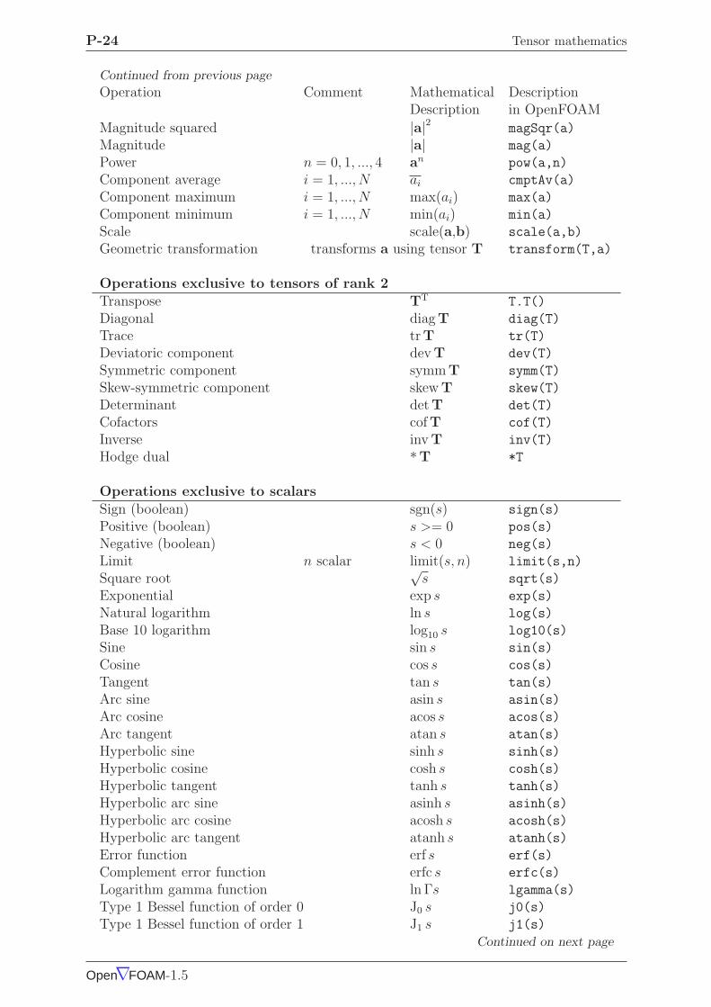
OpenFOAM supports most of the well known functions that operate on scalars, e.g. squareroot, exponential, logarithm, sine, cosine etc.., a list of which can be found in Table 1.2.There are 3 additional functions defined within OpenFOAM that are described below:
Sign of a scalar s is
sgn(s) =
1 if s ≥ 0,
−1 if s < 0.(1.41)
Positive of a scalar s is
pos(s) =
1 if s ≥ 0,
0 if s < 0.(1.42)
Limit of a scalar s by the scalar n
limit(s, n) =
s if s < n,
0 if s ≥ n.(1.43)
Open∇FOAM-1.5

1.4 OpenFOAM tensor classes P-23
1.4 OpenFOAM tensor classes
OpenFOAM contains a C++ class library primitive that contains the classes for the tensormathematics described so far. The basic tensor classes that are available as standard inOpenFOAM are listed in Table 1.1. The Table also lists the functions that allow the userto access individual components of a tensor, known as access functions.
Rank Common name Basic class Access functions0 Scalar scalar1 Vector vector x(), y(), z()2 Tensor tensor xx(), xy(), xz(). . .
Table 1.1: Basic tensor classes in OpenFOAM
We can declare the tensor
T =
1 2 34 5 67 8 9
(1.44)
in OpenFOAM by the line:
tensor T(1, 2, 3, 4, 5, 6, 7, 8, 9);
We can then access the component T13, or Txz using the xz() access function. Forinstance the code
Info << ‘‘Txz = ’’ << T.xz() << endl;
outputs to the screen:
Txz = 3
1.4.1 Algebraic tensor operations in OpenFOAM
The algebraic operations described in Section 1.3 are all available to the OpenFOAMtensor classes using syntax which closely mimics the notation used in written mathematics.Some functions are represented solely by descriptive functions, e.g.symm(), but others canalso be executed using symbolic operators, e.g.*. All functions are listed in Table 1.2.
Operation Comment Mathematical DescriptionDescription in OpenFOAM
Addition a + b a + b
Subtraction a − b a - b
Scalar multiplication sa s * a
Scalar division a/s a / s
Outer product rank a,b >= 1 ab a * b
Inner product rank a,b >= 1 a •b a & b
Double inner product rank a,b >= 2 a •
•b a && b
Cross product rank a,b = 1 a × b a ^ b
Square a2 sqr(a)
Continued on next page
Open∇FOAM-1.5
P-24 Tensor mathematics
Continued from previous page
Operation Comment Mathematical DescriptionDescription in OpenFOAM
Magnitude squared |a|2 magSqr(a)
Magnitude |a| mag(a)
Power n = 0, 1, ..., 4 an pow(a,n)
Component average i = 1, ..., N ai cmptAv(a)
Component maximum i = 1, ..., N max(ai) max(a)
Component minimum i = 1, ..., N min(ai) min(a)
Scale scale(a,b) scale(a,b)
Geometric transformation transforms a using tensor T transform(T,a)
Operations exclusive to tensors of rank 2Transpose TT T.T()
Diagonal diagT diag(T)
Trace trT tr(T)
Deviatoric component dev T dev(T)
Symmetric component symmT symm(T)
Skew-symmetric component skew T skew(T)
Determinant detT det(T)
Cofactors cofT cof(T)
Inverse inv T inv(T)
Hodge dual ∗T *T
Operations exclusive to scalarsSign (boolean) sgn(s) sign(s)
Positive (boolean) s >= 0 pos(s)
Negative (boolean) s < 0 neg(s)
Limit n scalar limit(s, n) limit(s,n)
Square root√
s sqrt(s)
Exponential exp s exp(s)
Natural logarithm ln s log(s)
Base 10 logarithm log10 s log10(s)
Sine sin s sin(s)
Cosine cos s cos(s)
Tangent tan s tan(s)
Arc sine asin s asin(s)
Arc cosine acos s acos(s)
Arc tangent atan s atan(s)
Hyperbolic sine sinh s sinh(s)
Hyperbolic cosine cosh s cosh(s)
Hyperbolic tangent tanh s tanh(s)
Hyperbolic arc sine asinh s asinh(s)
Hyperbolic arc cosine acosh s acosh(s)
Hyperbolic arc tangent atanh s atanh(s)
Error function erf s erf(s)
Complement error function erfc s erfc(s)
Logarithm gamma function ln Γs lgamma(s)
Type 1 Bessel function of order 0 J0 s j0(s)
Type 1 Bessel function of order 1 J1 s j1(s)
Continued on next page
Open∇FOAM-1.5
1.5 Dimensional units P-25
Continued from previous page
Operation Comment Mathematical DescriptionDescription in OpenFOAM
Type 2 Bessel function of order 0 Y0 s y0(s)
Type 2 Bessel function of order 1 Y1 s y1(s)
a,b are tensors of arbitrary rank unless otherwise stateds is a scalar, N is the number of tensor components
Table 1.2: Algebraic tensor operations in OpenFOAM
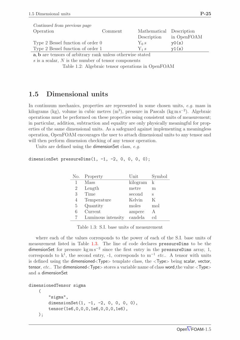
1.5 Dimensional units
In continuum mechanics, properties are represented in some chosen units, e.g. mass inkilograms (kg), volume in cubic metres (m3), pressure in Pascals (kg m s−2). Algebraicoperations must be performed on these properties using consistent units of measurement;in particular, addition, subtraction and equality are only physically meaningful for prop-erties of the same dimensional units. As a safeguard against implementing a meaninglessoperation, OpenFOAM encourages the user to attach dimensional units to any tensor andwill then perform dimension checking of any tensor operation.
Units are defined using the dimensionSet class, e.g.
dimensionSet pressureDims(1, -1, -2, 0, 0, 0, 0);
No. Property Unit Symbol1 Mass kilogram k2 Length metre m3 Time second s4 Temperature Kelvin K5 Quantity moles mol6 Current ampere A7 Luminous intensity candela cd
Table 1.3: S.I. base units of measurement
where each of the values corresponds to the power of each of the S.I. base units ofmeasurement listed in Table 1.3. The line of code declares pressureDims to be thedimensionSet for pressure kg m s−2 since the first entry in the pressureDims array, 1,corresponds to k1, the second entry, -1, corresponds to m−1 etc.. A tensor with unitsis defined using the dimensioned<Type> template class, the <Type> being scalar, vector,tensor, etc.. The dimensioned<Type> stores a variable name of class word,the value <Type>
and a dimensionSet
dimensionedTensor sigma
(
"sigma",
dimensionSet(1, -1, -2, 0, 0, 0, 0),
tensor(1e6,0,0,0,1e6,0,0,0,1e6),
);
Open∇FOAM-1.5

P-26 Tensor mathematics
creates a tensor with correct dimensions of pressure, or stress
σ =
106 0 00 106 00 0 106
(1.45)
Open∇FOAM-1.5

Chapter 2
Discretisation procedures
So far we have dealt with algebra of tensors at a point. The PDEs we wish to solve involvederivatives of tensors with respect to time and space. We therefore need to extend ourdescription to a tensor field, i.e. a tensor that varies across time and spatial domains.In this Chapter we will first present a mathematical description of all the differentialoperators we may encounter. We will then show how a tensor field is constructed inOpenFOAM and how the derivatives of these fields are discretised into a set of algebraicequations.
2.1 Differential operators
Before defining the spatial derivatives we first introduce the nabla vector operator ∇,represented in index notation as ∂i:
∇ ≡ ∂i ≡∂
∂xi
≡(
∂
∂x1
,∂
∂x2
,∂
∂x3
)
(2.1)
The nabla operator is a useful notation that obeys the following rules:
• it operates on the tensors to its right and the conventional rules of a derivative ofa product, e.g. ∂iab = (∂ia) b + a (∂ib);
• otherwise the nabla operator behaves like any other vector in an algebraic operation.
2.1.1 Gradient
If a scalar field s is defined and continuously differentiable then the gradient of s, ∇s isa vector field
∇s = ∂is =
(∂s
∂x1
,∂s
∂x2
,∂s
∂x3
)
(2.2)
The gradient can operate on any tensor field to produce a tensor field that is one rankhigher. For example, the gradient of a vector field a is a second rank tensor field
∇a = ∂iaj =
∂a1/∂x1 ∂a2/∂x1 ∂a3/∂x1
∂a1/∂x2 ∂a2/∂x2 ∂a3/∂x2
∂a1/∂x3 ∂a2/∂x3 ∂a3/∂x3
(2.3)
P-28 Discretisation procedures
2.1.2 Divergence
If a vector field a is defined and continuously differentiable then the divergence of a is ascalar field
∇ • a = ∂iai =∂a1
∂x1
+∂a2
∂x2
+∂a3
∂x3
(2.4)
The divergence can operate on any tensor field of rank 1 and above to produce atensor that is one rank lower. For example the divergence of a second rank tensor fieldT is a vector field (expanding the vector as a column array for convenience)
∇ •T = ∂iTij =
∂T11/∂x1 + ∂T12/∂x1 + ∂T13/∂x1
∂T21/∂x2 + ∂T22/∂x2 + ∂T23/∂x2
∂T31/∂x3 + ∂T32/∂x3 + ∂T33/∂x3
(2.5)
2.1.3 Curl
If a vector field a is defined and continuously differentiable then the curl of a, ∇× a is avector field
∇× a = eijk∂jak =
(∂a3
∂x2
− ∂a2
∂x3
,∂a1
∂x3
− ∂a3
∂x1
,∂a2
∂x1
− ∂a1
∂x2
)
(2.6)
The curl is related to the gradient by
∇× a = 2 (∗ skew∇a) (2.7)
2.1.4 Laplacian
The Laplacian is an operation that can be defined mathematically by a combination ofthe divergence and gradient operators by ∇2 ≡ ∇ •∇. However, the Laplacian should beconsidered as a single operation that transforms a tensor field into another tensor field ofthe same rank, rather than a combination of two operations, one which raises the rankby 1 and one which reduces the rank by 1.
In fact, the Laplacian is best defined as a scalar operator , just as we defined nabla asa vector operator, by
∇2 ≡ ∂2 ≡ ∂2
∂x21
+∂2
∂x22
+∂2
∂x23
(2.8)
For example, the Laplacian of a scalar field s is the scalar field
∇2s = ∂2s =∂2s
∂x21
+∂2s
∂x22
+∂2s
∂x23
(2.9)
2.1.5 Temporal derivative
There is more than one definition of temporal, or time, derivative of a tensor. To describethe temporal derivatives we must first recall that the tensor relates to a property of avolume of material that may be moving. If we track an infinitesimally small volume ofmaterial, or particle, as it moves and observe the change in the tensorial property φ intime, we have the total, or material time derivative denoted by
Dφ
Dt= lim
∆t→0
∆φ
∆t(2.10)
Open∇FOAM-1.5
2.2 Overview of discretisation P-29
However in continuum mechanics, particularly fluid mechanics, we often observe thechange of a φ in time at a fixed point in space as different particles move across thatpoint. This change at a point in space is termed the spatial time derivative which isdenoted by ∂/∂t and is related to the material derivative by:
Dφ
Dt=
∂φ
∂t+ U •∇φ (2.11)
where U is the velocity field of property φ. The second term on the right is known as theconvective rate of change of φ.
2.2 Overview of discretisation
The term discretisation means approximation of a problem into discrete quantities. TheFV method and others, such as the finite element and finite difference methods, alldiscretise the problem as follows:
Spatial discretisation Defining the solution domain by a set of points that fill andbound a region of space when connected;
Temporal discretisation (For transient problems) dividing the time domain into intoa finite number of time intervals, or steps;
Equation discretisation Generating a system of algebraic equations in terms of dis-crete quantities defined at specific locations in the domain, from the PDEs thatcharacterise the problem.
2.2.1 OpenFOAM lists and fields
OpenFOAM frequently needs to store sets of data and perform functions, such as mathe-matical operations, on the data. OpenFOAM therefore provides an array template classList<Type>, making it possible to create a list of any object of class Type that inheritsthe functions of the Type. For example a List of vector is List<vector>.
Lists of the tensor classes are defined as standard in OpenFOAM by the template classField<Type>. For better code legibility, all instances of Field<Type>, e.g.Field<vector>, arerenamed using typedef declarations as scalarField, vectorField, tensorField, symmTensor-Field, tensorThirdField and symmTensorThirdField. Algebraic operations can be performedbetween Fields subject to obvious restrictions such as the fields having the same numberof elements. OpenFOAM also supports operations between a field and single tensor, e.g.
all values of a Field U can be multiplied by the scalar 2 with the operation U = 2.0 * U.
2.3 Discretisation of the solution domain
Discretisation of the solution domain is shown in Figure 2.1. The space domain is discre-tised into computational mesh on which the PDEs are subsequently discretised. Discreti-sation of time, if required, is simple: it is broken into a set of time steps ∆t that maychange during a numerical simulation, perhaps depending on some condition calculatedduring the simulation.
On a more detailed level, discretisation of space requires the subdivision of the domaininto a number of cells, or control volumes. The cells are contiguous, i.e. they do notoverlap one another and completely fill the domain. A typical cell is shown in Figure 2.2.
Open∇FOAM-1.5

P-30 Discretisation procedures
z
y
xSpace domain
t
Time domain
∆t
Figure 2.1: Discretisation of the solution domain
N
SfP
f
d
Figure 2.2: Parameters in finite volume discretisation
Open∇FOAM-1.5

2.3 Discretisation of the solution domain P-31
Dependent variables and other properties are principally stored at the cell centroid Palthough they may be stored on faces or vertices. The cell is bounded by a set of flatfaces, given the generic label f . In OpenFOAM there is no limitation on the number offaces bounding each cell, nor any restriction on the alignment of each face. This kindof mesh is often referred to as “arbitrarily unstructured” to differentiate it from meshesin which the cell faces have a prescribed alignment, typically with the coordinate axes.Codes with arbitrarily unstructured meshes offer greater freedom in mesh generation andmanipulation in particular when the geometry of the domain is complex or changes overtime.
Whilst most properties are defined at the cell centroids, some are defined at cell faces.There are two types of cell face.
Internal faces Those faces that connect two cells (and it can never be more than two).For each internal face, OpenFOAM designates one adjoining cell to be the faceowner and the other to be the neighbour ;
Boundary faces Those belonging to one cell since they coincide with the boundary ofthe domain. These faces simply have an owner cell.
2.3.1 Defining a mesh in OpenFOAM
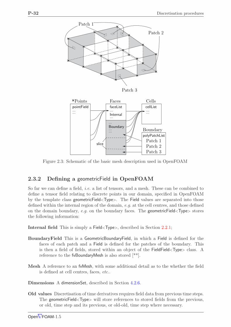
There are different levels of mesh description in OpenFOAM, beginning with the mostbasic mesh class, named polyMesh since it is based on polyhedra. A polyMesh is con-structed using the minimum information required to define the mesh geometry describedbelow and presented in Figure 2.3:
Points A list of cell vertex point coordinate vectors, i.e. a vectorField, that is renamedpointField using a typedef declaration;
Faces A list of cell faces List<face>, or faceList, where the face class is defined by a listof vertex numbers, corresponding to the pointField;
Cells a list of cells List<cell>, or cellList, where the cell class is defined by a list of facenumbers, corresponding to the faceList described previously.
Boundary a polyBoundaryMesh decomposed into a list of patches, polyPatchList rep-resenting different regions of the boundary. The boundary is subdivided in thismanner to allow different boundary conditions to be specified on different patchesduring a solution. All the faces of any polyPatch are stored as a single block of thefaceList, so that its faces can be easily accessed using the slice class which storesreferences to the first and last face of the block. Each polyPatch is then constructedfrom
• a slice;
• a word to assign it a name.
FV discretisation uses specific data that is derived from the mesh geometry storedin polyMesh. OpenFOAM therefore extends the polyMesh class to fvMesh which storesthe additional data needed for FV discretisation. fvMesh is constructed from polyMeshand stores the data in Table 2.1 which can be updated during runtime in cases where themesh moves, is refined etc..
Open∇FOAM-1.5
P-32 Discretisation procedures
Patch 3
Patch 2
pointField faceList
polyPatchList
Boundary
Patch 1Patch 2Patch 3
FacesPoints Cells
Internal...
Boundary......
...
slice
Patch 1
......... ...
...cellList
Figure 2.3: Schematic of the basic mesh description used in OpenFOAM
2.3.2 Defining a geometricField in OpenFOAM
So far we can define a field, i.e. a list of tensors, and a mesh. These can be combined todefine a tensor field relating to discrete points in our domain, specified in OpenFOAMby the template class geometricField<Type>. The Field values are separated into thosedefined within the internal region of the domain, e.g. at the cell centres, and those definedon the domain boundary, e.g. on the boundary faces. The geometricField<Type> storesthe following information:
Internal field This is simply a Field<Type>, described in Section 2.2.1;
BoundaryField This is a GeometricBoundaryField, in which a Field is defined for thefaces of each patch and a Field is defined for the patches of the boundary. Thisis then a field of fields, stored within an object of the FieldField<Type> class. Areference to the fvBoundaryMesh is also stored [**].
Mesh A reference to an fvMesh, with some additional detail as to the whether the fieldis defined at cell centres, faces, etc..
Dimensions A dimensionSet, described in Section 4.2.6.
Old values Discretisation of time derivatives requires field data from previous time steps.The geometricField<Type> will store references to stored fields from the previous,or old, time step and its previous, or old-old, time step where necessary.
Open∇FOAM-1.5

2.4 Equation discretisation P-33
Class Description Symbol Access function
volScalarField Cell volumes V V()
surfaceVectorField Face area vectors Sf Sf()
surfaceScalarField Face area magnitudes |Sf | magSf()
volVectorField Cell centres C C()
surfaceVectorField Face centres Cf Cf()
surfaceScalarField Face motion fluxes ** φg phi()
Table 2.1: fvMesh stored data.
Previous iteration values The iterative solution procedures can use under-relaxationwhich requires access to data from the previous iteration. Again, if required, geo-metricField<Type> stores a reference to the data from the previous iteration.
As discussed in Section 2.3, we principally define a property at the cell centres but quiteoften it is stored at the cell faces and on occasion it is defined on cell vertices. ThegeometricField<Type> is renamed using typedef declarations to indicate where the fieldvariable is defined as follows:
volField<Type> A field defined at cell centres;
surfaceField<Type> A field defined on cell faces;
pointField<Type> A field defined on cell vertices.
These typedef field classes of geometricField<Type>are illustrated in Figure 2.4. AgeometricField<Type> inherits all the tensor algebra of Field<Type> and has all operationssubjected to dimension checking using the dimensionSet. It can also be subjected to theFV discretisation procedures described in the following Section. The class structure usedto build geometricField<Type> is shown in Figure 2.51.
2.4 Equation discretisation
Equation discretisation converts the PDEs into a set of algebraic equations that arecommonly expressed in matrix form as:
[A] [x] = [b] (2.12)
where [A] is a square matrix, [x] is the column vector of dependent variable and [b] isthe source vector. The description of [x] and [b] as ‘vectors’ comes from matrix termi-nology rather than being a precise description of what they truly are: a list of valuesdefined at locations in the geometry, i.e. a geometricField<Type>, or more specifically avolField<Type> when using FV discretisation.
[A] is a list of coefficients of a set of algebraic equations, and cannot be described as ageometricField<Type>. It is therefore given a class of its own: fvMatrix. fvMatrix<Type>
is created through discretisation of a geometric<Type>Field and therefore inherits the<Type>. It supports many of the standard algebraic matrix operations of addition +,subtraction - and multiplication *.
Each term in a PDE is represented individually in OpenFOAM code using the classesof static functions finiteVolumeMethod and finiteVolumeCalculus, abbreviated by a typedef
1The diagram is not an exact description of the class hierarchy, rather a representation of the generalstructure leading from some primitive classes to geometric<Type>Field.
Open∇FOAM-1.5

P-34 Discretisation procedures
Internal field
Boundary fieldPatch 1Patch 2
Patch 1
Patch 2
(a) A volField<Type>
Internal field
Boundary fieldPatch 1Patch 2
Patch 1
Patch 2
(b) A surfaceField<Type>
Internal field
Boundary fieldPatch 1Patch 2
Patch 1
Patch 2
(c) A pointField<Type>
Figure 2.4: Types of geometricField<Type> defined on a mesh with 2 boundary patches(in 2 dimensions for simplicity)
Open∇FOAM-1.5

2.4 Equation discretisation P-35
polyMesh
labelList
<Type>
scalarvectortensorsymmTensortensorThirdsymmTensorThird
dimensioned<Type>
cell
fvBoundaryMesh
polyBoundaryMesh
polyPatch
slice
polyPatchListcellListfaceList
face
fvPatchList
fvPatch
List
pointField
wordlabel
fvMesh
geometricField<Type>
Field<Type>
fvPatchField
dimensionSet
geometricBoundaryField<Type>
Figure 2.5: Basic class structure leading to geometricField<Type>
Open∇FOAM-1.5
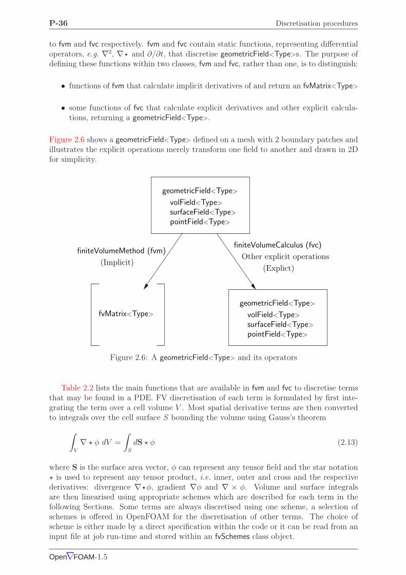
P-36 Discretisation procedures
to fvm and fvc respectively. fvm and fvc contain static functions, representing differentialoperators, e.g. ∇2, ∇ • and ∂/∂t, that discretise geometricField<Type>s. The purpose ofdefining these functions within two classes, fvm and fvc, rather than one, is to distinguish:
• functions of fvm that calculate implicit derivatives of and return an fvMatrix<Type>
• some functions of fvc that calculate explicit derivatives and other explicit calcula-tions, returning a geometricField<Type>.
Figure 2.6 shows a geometricField<Type> defined on a mesh with 2 boundary patches andillustrates the explicit operations merely transform one field to another and drawn in 2Dfor simplicity.
geometricField<Type>
volField<Type>
surfaceField<Type>
pointField<Type>
geometricField<Type>
volField<Type>
surfaceField<Type>
pointField<Type>
fvMatrix<Type>
finiteVolumeMethod (fvm)
(Implicit)
finiteVolumeCalculus (fvc)
Other explicit operations
(Explict)
Figure 2.6: A geometricField<Type> and its operators
Table 2.2 lists the main functions that are available in fvm and fvc to discretise termsthat may be found in a PDE. FV discretisation of each term is formulated by first inte-grating the term over a cell volume V . Most spatial derivative terms are then convertedto integrals over the cell surface S bounding the volume using Gauss’s theorem
∫
V
∇ ⋆ φ dV =
∫
S
dS ⋆ φ (2.13)
where S is the surface area vector, φ can represent any tensor field and the star notation⋆ is used to represent any tensor product, i.e. inner, outer and cross and the respectivederivatives: divergence ∇ • φ, gradient ∇φ and ∇ × φ. Volume and surface integralsare then linearised using appropriate schemes which are described for each term in thefollowing Sections. Some terms are always discretised using one scheme, a selection ofschemes is offered in OpenFOAM for the discretisation of other terms. The choice ofscheme is either made by a direct specification within the code or it can be read from aninput file at job run-time and stored within an fvSchemes class object.
Open∇FOAM-1.5

2.4 Equation discretisation P-37
Term description Implicit / Text fvm::/fvc:: functionsExplicit expression
Laplacian Imp/Exp ∇2φ laplacian(phi)
∇ • Γ∇φ laplacian(Gamma, phi)
Time derivative Imp/Exp∂φ
∂tddt(phi)
∂ρφ
∂tddt(rho,phi)
Second time derivative Imp/Exp∂
∂t
(
ρ∂φ
∂t
)
d2dt2(rho, phi)
Convection Imp/Exp ∇ • (ψ) div(psi,scheme)*∇ • (ψφ) div(psi, phi, word)*
div(psi, phi)
Divergence Exp ∇ • χ div(chi)
Gradient Exp ∇χ grad(chi)
∇φ gGrad(phi)
lsGrad(phi)
snGrad(phi)
snGradCorrection(phi)
Grad-grad squared Exp |∇∇φ|2 sqrGradGrad(phi)
Curl Exp ∇× φ curl(phi)
Source Imp ρφ Sp(rho,phi)
Imp/Exp† SuSp(rho,phi)
†fvm::SuSp source is discretised implicit or explicit depending on the sign of rho.†An explicit source can be introduced simply as a vol<Type>Field, e.g.rho*phi.Function arguments can be of the following classes:phi: vol<Type>FieldGamma: scalar volScalarField, surfaceScalarField, volTensorField, surfaceTensorField.rho: scalar, volScalarFieldpsi: surfaceScalarField.chi: surface<Type>Field, vol<Type>Field.
Table 2.2: Discretisation of PDE terms in OpenFOAM
Open∇FOAM-1.5
P-38 Discretisation procedures
2.4.1 The Laplacian term
The Laplacian term is integrated over a control volume and linearised as follows:
∫
V
∇ • (Γ∇φ) dV =
∫
S
dS • (Γ∇φ) =∑
f
ΓfSf • (∇φ)f (2.14)
The face gradient discretisation is implicit when the length vector d between the centreof the cell of interest P and the centre of a neighbouring cell N is orthogonal to the faceplane, i.e. parallel to Sf :
Sf • (∇φ)f = |Sf |φN − φP
|d| (2.15)
In the case of non-orthogonal meshes, an additional explicit term is introduced [?] whichis evaluated by interpolating cell centre gradients, themselves calculated by central dif-ferencing cell centre values.
2.4.2 The convection term
The convection term is integrated over a control volume and linearised as follows:
∫
V
∇ • (ρUφ) dV =
∫
S
dS • (ρUφ) =∑
f
Sf • (ρU)fφf =∑
f
Fφf (2.16)
The face field φf can be evaluated using a variety of schemes:
Central differencing (CD) is second-order accurate but unbounded
φf = fxφP + (1 − fx)φN (2.17)
where fx ≡ fN/PN where fN is the distance between f and cell centre N andPN is the distance between cell centres P and N .
Upwind differencing (UD) determines φf from the direction of flow and is boundedat the expense of accuracy
φf =
φP for F ≥ 0
φN for F < 0(2.18)
Blended differencing (BD) schemes combine UD and CD in an attempt to preserveboundedness with reasonable accuracy,
φf = (1 − γ) (φf )UD+ γ (φf )CD
(2.19)
OpenFOAM has several implementations of the Gamma differencing scheme toselect the blending coefficient γ [?] but it offers other well-known schemes such asvan Leer, SUPERBEE, MINMOD etc..
Open∇FOAM-1.5
2.4 Equation discretisation P-39
2.4.3 First time derivative
The first time derivative ∂/∂t is integrated over a control volume as follows:
∂
∂t
∫
V
ρφ dV (2.20)
The term is discretised by simple differencing in time using:
new values φn ≡ φ(t + ∆t) at the time step we are solving for;
old values φo ≡ φ(t) that were stored from the previous time step;
old-old values φoo ≡ φ(t − ∆t) stored from a time step previous to the last.
One of two discretisation schemes can be declared using the timeScheme keyword in theappropriate input file, described in detail in section 4.4 of the User Guide.
Euler implicit scheme, timeScheme EulerImplicit, that is first order accurate in time:
∂
∂t
∫
V
ρφ dV =(ρP φP V )n − (ρP φP V )o
∆t(2.21)
Backward differencing scheme, timeScheme BackwardDifferencing, that is secondorder accurate in time by storing the old-old values and therefore with a largeroverhead in data storage than EulerImplicit:
∂
∂t
∫
V
ρφ dV =3 (ρP φP V )n − 4 (ρP φP V )o + (ρP φP V )oo
2∆t(2.22)
2.4.4 Second time derivative
The second time derivative is integrated over a control volume and linearised as follows:
∂
∂t
∫
V
ρ∂φ
∂tdV =
(ρP φP V )n − 2 (ρP φP V )o + (ρP φP V )oo
∆t2(2.23)
It is first order accurate in time.
2.4.5 Divergence
The divergence term described in this Section is strictly an explicit term that is distin-guished from the convection term of Section 2.4.2, i.e. in that it is not the divergence ofthe product of a velocity and dependent variable. The term is integrated over a controlvolume and linearised as follows:
∫
V
∇ • φ dV =
∫
S
dS • φ =∑
f
Sf • φf (2.24)
The fvc::div function can take as its argument either a surface<Type>Field, in whichcase φf is specified directly, or a vol<Type>Field which is interpolated to the face bycentral differencing as described in Section 2.4.10:
Open∇FOAM-1.5

P-40 Discretisation procedures
2.4.6 Gradient
The gradient term is an explicit term that can be evaluated in a variety of ways. Thescheme can be evaluated either by selecting the particular grad function relevant to thediscretisation scheme, e.g.fvc::gGrad, fvc::lsGrad etc., or by using the fvc::grad
function combined with the appropriate timeScheme keyword in an input file
Gauss integration is invoked using the fvc::grad function with timeScheme Gauss
or directly using the fvc::gGrad function. The discretisation is performed usingthe standard method of applying Gauss’s theorem to the volume integral:
∫
V
∇φ dV =
∫
S
dSφ =∑
f
Sfφf (2.25)
As with the fvc::div function, the Gaussian integration fvc::grad function cantake either a surfaceField<Type> or a volField<Type> as an argument.
Least squares method is based on the following idea:
1. a value at point P can be extrapolated to neighbouring point N using thegradient at P ;
2. the extrapolated value at N can be compared to the actual value at N , thedifference being the error;
3. if we now minimise the sum of the square of weighted errors at all neighboursof P with the respect to the gradient, then the gradient should be a goodapproximation.
Least squares is invoked using the fvc::grad function with timeScheme leastSquares
or directly using the fvc::lsGrad function. The discretisation is performed as byfirst calculating the tensor G at every point P by summing over neighbours N :
G =∑
N
w2Ndd (2.26)
where d is the vector from P to N and the weighting function wN = 1/|d|. Thegradient is then evaluated as:
(∇φ)P =∑
N
w2NG−1
•d (φN − φP ) (2.27)
Surface normal gradient The gradient normal to a surface nf • (∇φ)f can be evalu-ated at cell faces using the scheme
(∇φ)f =φN − φP
|d| (2.28)
This gradient is called by the function fvc::snGrad and returns a surfaceField<Type>.The scheme is directly analogous to that evaluated for the Laplacian discretisationscheme in Section 2.4.1, and in the same manner, a correction can be introducedto improve the accuracy of this face gradient in the case of non-orthogonal meshes.This correction is called using the function fvc::snGradCorrection [Check**].
Open∇FOAM-1.5

2.4 Equation discretisation P-41
2.4.7 Grad-grad squared
The grad-grad squared term is evaluated by: taking the gradient of the field; taking thegradient of the resulting gradient field; and then calculating the magnitude squared ofthe result. The mathematical expression for grad-grad squared of φ is |∇ (∇φ)|2.
2.4.8 Curl
The curl is evaluated from the gradient term described in Section 2.4.6. First, the gradientis discretised and then the curl is evaluated using the relationship from Equation 2.7,repeated here for convenience
∇× φ = 2 ∗(skew∇φ)
2.4.9 Source terms
Source terms can be specified in 3 ways
Explicit Every explicit term is a volField<Type>. Hence, an explicit source term can beincorporated into an equation simply as a field of values. For example if we wishedto solve Poisson’s equation ∇2φ = f , we would define phi and f as volScalarFieldand then do
solve(fvm::laplacian(phi) == f)
Implicit An implicit source term is integrated over a control volume and linearised by
∫
V
ρφ dV = ρP VP φP (2.29)
Implicit/Explicit The implicit source term changes the coefficient of the diagonal ofthe matrix. Depending on the sign of the coefficient and matrix terms, this willeither increase or decrease diagonal dominance of the matrix. Decreasing the di-agonal dominance could cause instability during iterative solution of the matrixequation. Therefore OpenFOAM provides a mixed source discretisation procedurethat is implicit when the coefficients that are greater than zero, and explicit for thecoefficients less than zero. In mathematical terms the matrix coefficient for node Pis VP max(ρP , 0) and the source term is VP φP min(ρP , 0).
2.4.10 Other explicit discretisation schemes
There are some other discretisation procedures that convert volField<Type>s into sur-face<Type>Fields and visa versa.
Surface integral fvc::surfaceIntegrate performs a summation of surface<Type>Fieldface values bounding each cell and dividing by the cell volume, i.e. (
∑
f φf )/VP . Itreturns a volField<Type>.
Surface sum fvc::surfaceSum performs a summation of surface<Type>Field face val-ues bounding each cell, i.e.
∑
f φf returning a volField<Type>.
Average fvc::average produces an area weighted average of surface<Type>Field facevalues, i.e. (
∑
f Sfφf )/∑
f Sf , and returns a volField<Type>.
Open∇FOAM-1.5
P-42 Discretisation procedures
Reconstruct
Face interpolate The geometric<Type>Field function faceInterpolate() interpolatesvolField<Type> cell centre values to cell faces using central differencing, returning asurface<Type>Field.
2.5 Temporal discretisation
Although we have described the discretisation of temporal derivatives in Sections 2.4.3and 2.4.4, we need to consider how to treat the spatial derivatives in a transient problem.If we denote all the spatial terms as Aφ where A is any spatial operator, e.g. Laplacian,then we can express a transient PDE in integral form as
∫ t+∆t
t
[∂
∂t
∫
V
ρφ dV +
∫
V
Aφ dV
]
dt = 0 (2.30)
Using the Euler implicit method of Equation 2.21, the first term can be expressed as∫ t+∆t
t
[∂
∂t
∫
V
ρφ dV
]
dt =
∫ t+∆t
t
(ρP φP V )n − (ρP φP V )o
∆tdt
=(ρP φP V )n − (ρP φP V )o
∆t∆t
(2.31)
The second term can be expressed as∫ t+∆t
t
[∫
V
Aφ dV
]
dt =
∫ t+∆t
t
A∗φ dt (2.32)
where A∗ represents the spatial discretisation of A. The time integral can be discretisedin three ways:
Euler implicit uses implicit discretisation of the spatial terms, thereby taking currentvalues φn.
∫ t+∆t
t
A∗φ dt = A∗φn∆t (2.33)
It is first order accurate in time, guarantees boundedness and is unconditionallystable.
Explicit uses explicit discretisation of the spatial terms, thereby taking old values φo.∫ t+∆t
t
A∗φ dt = A∗φo∆t (2.34)
It is first order accurate in time and is unstable if the Courant number Co is greaterthan 1. The Courant number is defined as
Co =Uf •d
|d|2∆t(2.35)
where Uf is a characteristic velocity, e.g. velocity of a wave front, velocity of flow.
Crank Nicholson uses the trapezoid rule to discretise the spatial terms, thereby takinga mean of current values φn and old values φo.
∫ t+∆t
t
A∗φ dt = A∗
(φn + φo
2
)
∆t (2.36)
It is second order accurate in time, is unconditionally stable but does not guaranteeboundedness.
Open∇FOAM-1.5

2.6 Boundary Conditions P-43
2.5.1 Treatment of temporal discretisation in OpenFOAM
At present the treatment of the temporal discretisation is controlled by the implementa-tion of the spatial derivatives in the PDE we wish to solve. For example, let us say wewish to solve a transient diffusion equation
∂φ
∂t= κ∇2φ (2.37)
An Euler implicit implementation of this would read
solve(fvm::ddt(phi) == kappa*fvm::laplacian(phi))
where we use the fvm class to discretise the Laplacian term implicitly. An explicitimplementation would read
solve(fvm::ddt(phi) == kappa*fvc::laplacian(phi))
where we now use the fvc class to discretise the Laplacian term explicitly. The CrankNicholson scheme can be implemented by the mean of implicit and explicit terms:
solve
(
fvm::ddt(phi)
==
kappa*0.5*(fvm::laplacian(phi) + fvc::laplacian(phi))
)
2.6 Boundary Conditions
Boundary conditions are required to complete the problem we wish to solve. We thereforeneed to specify boundary conditions on all our boundary faces. Boundary conditions canbe divided into 2 types:
Dirichlet prescribes the value of the dependent variable on the boundary and is thereforetermed ‘fixed value’ in this guide;
Neumann prescribes the gradient of the variable normal to the boundary and is thereforetermed ‘fixed gradient’ in this guide.
When we perform discretisation of terms that include the sum over faces∑
f , we needto consider what happens when one of the faces is a boundary face.
Fixed value We specify a fixed value at the boundary φb
• We can simply substitute φb in cases where the discretisation requires the valueon a boundary face φf , e.g. in the convection term in Equation 2.16.
• In terms where the face gradient (∇φ)f is required, e.g. Laplacian, it is calcu-lated using the boundary face value and cell centre value,
Sf • (∇φ)f = |Sf |φb − φP
|d| (2.38)
Open∇FOAM-1.5
P-44 Discretisation procedures
Fixed gradient The fixed gradient boundary condition gb is a specification on innerproduct of the gradient and unit normal to the boundary, or
gb =
(S
|S|•∇φ
)
f
(2.39)
• When discretisation requires the value on a boundary face φf we must inter-polate the cell centre value to the boundary by
φf = φP + d • (∇φ)f
= φP + |d| gb
(2.40)
• φb can be directly substituted in cases where the discretisation requires theface gradient to be evaluated,
Sf • (∇φ)f = |Sf | gb (2.41)
2.6.1 Physical boundary conditions
The specification of boundary conditions is usually an engineer’s interpretation of thetrue behaviour. Real boundary conditions are generally defined by some physical at-tributes rather than the numerical description as described of the previous Section. Inincompressible fluid flow there are the following physical boundaries
Inlet The velocity field at the inlet is supplied and, for consistency, the boundary con-dition on pressure is zero gradient.
Outlet The pressure field at the outlet is supplied and a zero gradient boundary conditionon velocity is specified.
No-slip impermeable wall The velocity of the fluid is equal to that of the wall itself,i.e. a fixed value condition can be specified. The pressure is specified zero gradientsince the flux through the wall is zero.
In a problem whose solution domain and boundary conditions are symmetric about aplane, we only need to model half the domain to one side of the symmetry plane. Theboundary condition on the plane must be specified according to
Symmetry plane The symmetry plane condition specifies the component of the gradi-ent normal to the plane should be zero. [Check**]
Open∇FOAM-1.5

Chapter 3
Examples of the use of OpenFOAM
In this section we shall describe several test cases supplied with the OpenFOAM distri-bution. The intention is to provide example cases, including those in the tutorials inchapter 2 of the User Guide, for every standard solver. The examples are designed tointroduce certain tools and features of OpenFOAM, e.g. within pre-/post-processing, nu-merical schemes, algorithms. They also provide a means for validation of solvers althoughthat is not their principal function.
Each example contains a description of the problem: the geometry, initial and bound-ary conditions, a brief description of the equations being solved, models used, and physicalproperties required. The solution domain is selected which may be a portion of the orig-inal geometry, e.g. if we introduce symmetry planes. The method of meshing, usuallyblockMesh, is specified; of course the user can simply view the mesh since every exam-ple is distributed with the polyMesh directory containing the data files that describe themesh.
The examples coexist with the tutorials in the tutorials subdirectory of the OpenFOAMinstallation. They are organised into a set of subdirectories by solver, e.g. all the icoFoamcases are stored within a subdirectory icoFoam. Before running a particular example,the user is urged to copy it into their user account. We recommend that the user storesall OpenFOAM cases in a directory we recommend that the tutorials are copied into adirectory $FOAM RUN. If this directory structure has not yet been created in the user’saccount, it can be created with
mkdir -p $FOAM RUN
The tutorials can then be copied into this directory with
cp -r $FOAM TUTORIALS/* $FOAM RUN
3.1 Flow around a cylinder
In this example we shall investigate potential flow around a cylinder using potentialFoam.This example introduces the following OpenFOAM features:
• non-orthogonal meshes;
• generating an analytical solution to a problem in OpenFOAM.
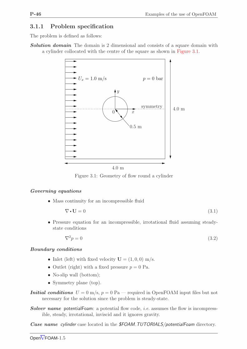
P-46 Examples of the use of OpenFOAM
3.1.1 Problem specification
The problem is defined as follows:
Solution domain The domain is 2 dimensional and consists of a square domain witha cylinder collocated with the centre of the square as shown in Figure 3.1.
Ux = 1.0 m/s p = 0 bar
symmetry
0.5 m
4.0 m
4.0 mx
y
0
Figure 3.1: Geometry of flow round a cylinder
Governing equations
• Mass continuity for an incompressible fluid
∇ •U = 0 (3.1)
• Pressure equation for an incompressible, irrotational fluid assuming steady-state conditions
∇2p = 0 (3.2)
Boundary conditions
• Inlet (left) with fixed velocity U = (1, 0, 0) m/s.
• Outlet (right) with a fixed pressure p = 0 Pa.
• No-slip wall (bottom);
• Symmetry plane (top).
Initial conditions U = 0 m/s, p = 0 Pa — required in OpenFOAM input files but notnecessary for the solution since the problem is steady-state.
Solver name potentialFoam: a potential flow code, i.e. assumes the flow is incompress-ible, steady, irrotational, inviscid and it ignores gravity.
Case name cylinder case located in the $FOAM TUTORIALS/potentialFoam directory.
Open∇FOAM-1.5
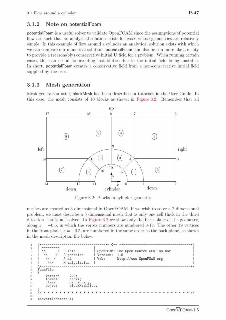
3.1 Flow around a cylinder P-47
3.1.2 Note on potentialFoam
potentialFoam is a useful solver to validate OpenFOAM since the assumptions of potentialflow are such that an analytical solution exists for cases whose geometries are relativelysimple. In this example of flow around a cylinder an analytical solution exists with whichwe can compare our numerical solution. potentialFoam can also be run more like a utilityto provide a (reasonably) conservative initial U field for a problem. When running certaincases, this can useful for avoiding instabilities due to the initial field being unstable.In short, potentialFoam creates a conservative field from a non-conservative initial fieldsupplied by the user.
3.1.3 Mesh generation
Mesh generation using blockMesh has been described in tutorials in the User Guide. Inthis case, the mesh consists of 10 blocks as shown in Figure 3.2. Remember that all
10
5
4
9
10
3
81817
16
1514
111213 2
7 6
2
3
0
1
4
5
67
89
y
xdown down
left right
cylinder
up
Figure 3.2: Blocks in cylinder geometry
meshes are treated as 3 dimensional in OpenFOAM. If we wish to solve a 2 dimensionalproblem, we must describe a 3 dimensional mesh that is only one cell thick in the thirddirection that is not solved. In Figure 3.2 we show only the back plane of the geometry,along z = −0.5, in which the vertex numbers are numbered 0-18. The other 19 verticesin the front plane, z = +0.5, are numbered in the same order as the back plane, as shownin the mesh description file below:
1 /*--------------------------------*- C++ -*----------------------------------*\2 | ========= | |3 | \\ / F ield | OpenFOAM: The Open Source CFD Toolbox |4 | \\ / O peration | Version: 1.5 |5 | \\ / A nd | Web: http://www.OpenFOAM.org |6 | \\/ M anipulation | |7 \*---------------------------------------------------------------------------*/8 FoamFile9
10 version 2.0;11 format ascii;12 class dictionary;13 object blockMeshDict;14 15 // * * * * * * * * * * * * * * * * * * * * * * * * * * * * * * * * * * * * * //16
17 convertToMeters 1;
Open∇FOAM-1.5

P-48 Examples of the use of OpenFOAM
18
19 vertices20 (21 (0.5 0 -0.5)22 (1 0 -0.5)23 (2 0 -0.5)24 (2 0.707107 -0.5)25 (0.707107 0.707107 -0.5)26 (0.353553 0.353553 -0.5)27 (2 2 -0.5)28 (0.707107 2 -0.5)29 (0 2 -0.5)30 (0 1 -0.5)31 (0 0.5 -0.5)32 (-0.5 0 -0.5)33 (-1 0 -0.5)34 (-2 0 -0.5)35 (-2 0.707107 -0.5)36 (-0.707107 0.707107 -0.5)37 (-0.353553 0.353553 -0.5)38 (-2 2 -0.5)39 (-0.707107 2 -0.5)40 (0.5 0 0.5)41 (1 0 0.5)42 (2 0 0.5)43 (2 0.707107 0.5)44 (0.707107 0.707107 0.5)45 (0.353553 0.353553 0.5)46 (2 2 0.5)47 (0.707107 2 0.5)48 (0 2 0.5)49 (0 1 0.5)50 (0 0.5 0.5)51 (-0.5 0 0.5)52 (-1 0 0.5)53 (-2 0 0.5)54 (-2 0.707107 0.5)55 (-0.707107 0.707107 0.5)56 (-0.353553 0.353553 0.5)57 (-2 2 0.5)58 (-0.707107 2 0.5)59 );60
61 blocks62 (63 hex (5 4 9 10 24 23 28 29) (10 10 1) simpleGrading (1 1 1)64 hex (0 1 4 5 19 20 23 24) (10 10 1) simpleGrading (1 1 1)65 hex (1 2 3 4 20 21 22 23) (20 10 1) simpleGrading (1 1 1)66 hex (4 3 6 7 23 22 25 26) (20 20 1) simpleGrading (1 1 1)67 hex (9 4 7 8 28 23 26 27) (10 20 1) simpleGrading (1 1 1)68 hex (15 16 10 9 34 35 29 28) (10 10 1) simpleGrading (1 1 1)69 hex (12 11 16 15 31 30 35 34) (10 10 1) simpleGrading (1 1 1)70 hex (13 12 15 14 32 31 34 33) (20 10 1) simpleGrading (1 1 1)71 hex (14 15 18 17 33 34 37 36) (20 20 1) simpleGrading (1 1 1)72 hex (15 9 8 18 34 28 27 37) (10 20 1) simpleGrading (1 1 1)73 );74
75 edges76 (77 arc 0 5 (0.469846 0.17101 -0.5)78 arc 5 10 (0.17101 0.469846 -0.5)79 arc 1 4 (0.939693 0.34202 -0.5)80 arc 4 9 (0.34202 0.939693 -0.5)81 arc 19 24 (0.469846 0.17101 0.5)82 arc 24 29 (0.17101 0.469846 0.5)83 arc 20 23 (0.939693 0.34202 0.5)84 arc 23 28 (0.34202 0.939693 0.5)85 arc 11 16 (-0.469846 0.17101 -0.5)86 arc 16 10 (-0.17101 0.469846 -0.5)87 arc 12 15 (-0.939693 0.34202 -0.5)88 arc 15 9 (-0.34202 0.939693 -0.5)89 arc 30 35 (-0.469846 0.17101 0.5)90 arc 35 29 (-0.17101 0.469846 0.5)91 arc 31 34 (-0.939693 0.34202 0.5)92 arc 34 28 (-0.34202 0.939693 0.5)93 );94
95 patches96 (97 symmetryPlane down98 (99 (0 1 20 19)
100 (1 2 21 20)101 (12 11 30 31)
Open∇FOAM-1.5

3.1 Flow around a cylinder P-49
102 (13 12 31 32)103 )104 patch right105 (106 (2 3 22 21)107 (3 6 25 22)108 )109 symmetryPlane up110 (111 (7 8 27 26)112 (6 7 26 25)113 (8 18 37 27)114 (18 17 36 37)115 )116 patch left117 (118 (14 13 32 33)119 (17 14 33 36)120 )121 symmetryPlane cylinder122 (123 (10 5 24 29)124 (5 0 19 24)125 (16 10 29 35)126 (11 16 35 30)127 )128 );129
130 mergePatchPairs131 (132 );133
134 // ************************************************************************* //
3.1.4 Boundary conditions and initial fields
Using FoamX or editing case files by hand, set the boundary conditions in accordancewith the problem description in Figure 3.1, i.e. the left boundary should be an Inlet,the right boundary should be an Outlet and the down and cylinder boundaries shouldbe symmetryPlane. The top boundary conditions is chosen so that we can make themost genuine comparison with our analytical solution which uses the assumption thatthe domain is infinite in the y direction. The result is that the normal gradient of U issmall along a plane coinciding with our boundary. We therefore impose the conditionthat the normal component is zero, i.e. specify the boundary as a symmetryPlane, therebyensuring that the comparison with the analytical is reasonable.
3.1.5 Running the case
No fluid properties need be specified in this problem since the flow is assumed to beincompressible and inviscid. In the system subdirectory, the controlDict specifies thecontrol parameters for the run. Note that since we assume steady flow, we only run for1 time step:
1 /*--------------------------------*- C++ -*----------------------------------*\2 | ========= | |3 | \\ / F ield | OpenFOAM: The Open Source CFD Toolbox |4 | \\ / O peration | Version: 1.5 |5 | \\ / A nd | Web: http://www.OpenFOAM.org |6 | \\/ M anipulation | |7 \*---------------------------------------------------------------------------*/8 FoamFile9
10 version 2.0;11 format ascii;12 class dictionary;13 object controlDict;14 15 // * * * * * * * * * * * * * * * * * * * * * * * * * * * * * * * * * * * * * //16
17 application potentialFoam;18
Open∇FOAM-1.5

P-50 Examples of the use of OpenFOAM
19 startFrom startTime;20
21 startTime 0;22
23 stopAt endTime;24
25 endTime 1;26
27 deltaT 1;28
29 writeControl timeStep;30
31 writeInterval 1;32
33 purgeWrite 0;34
35 writeFormat ascii;36
37 writePrecision 6;38
39 writeCompression uncompressed;40
41 timeFormat general;42
43 timePrecision 6;44
45 runTimeModifiable yes;46
47 // ************************************************************************* //
potentialFoam executes an iterative loop around the pressure equation which it solves inorder that explicit terms relating to non-orthogonal correction in the Laplacian term maybe updated in successive iterations. The number of iterations around the pressure equa-tion is controlled by the nNonOrthogonalCorrectors keyword in controlDict. In the firstinstance we can set nNonOrthogonalCorrectors to 0 so that no loops are performed,i.e. the pressure equation is solved once, and there is no non-orthogonal correction. Thesolution is shown in Figure 3.3(a) (at t = 1, when the steady-state simulation is com-plete). We expect the solution to show smooth streamlines passing across the domainas in the analytical solution in Figure 3.3(c), yet there is clearly some error in the re-gions where there is high non-orthogonality in the mesh, e.g. at the join of blocks 0, 1and 3. The case can be run a second time with some non-orthogonal correction by set-ting nNonOrthogonalCorrectors to 3. The solution shows smooth streamlines with nosignificant error due to non-orthogonality as shown in Figure 3.3(b).
3.1.6 Generating the analytical solution
Source code is included in the $FOAM TUTORIALS/potentialFoam/analyticalCylinder di-rectory to generate the analytical solution for the potential flow case. The velocity at anypoint at a distance d and angle θ from the cylinder centre is described analytically as
Ux = U∞
[
1 −(r
d
)2
cos 2θ
]
Uy = U∞
(r
d
)2
sin 2θ (3.3)
where r is the cylinder radius and U∞ is the inlet flow velocity. Here, θ describes theangle subtended from the x-axis.
Let us examine some details of the source code in the analyticalCylinder directory. IncreateFields.H, the velocity field is read in using the IOobject::NO WRITE option to ensurethat the field data can never be overwritten during execution of analyticalCylinder. Theinlet velocity and cylinder radius are taken from data read from the mesh and a field UA
is set up to store the analytical solution:
1 Info<< "Reading field U\n" << endl;2 volVectorField U
Open∇FOAM-1.5

3.1 Flow around a cylinder P-51
(a) With no non-orthogonal correction
(b) With non-orthogonal correction
(c) Analytical solution
Figure 3.3: Streamlines of potential flow
Open∇FOAM-1.5
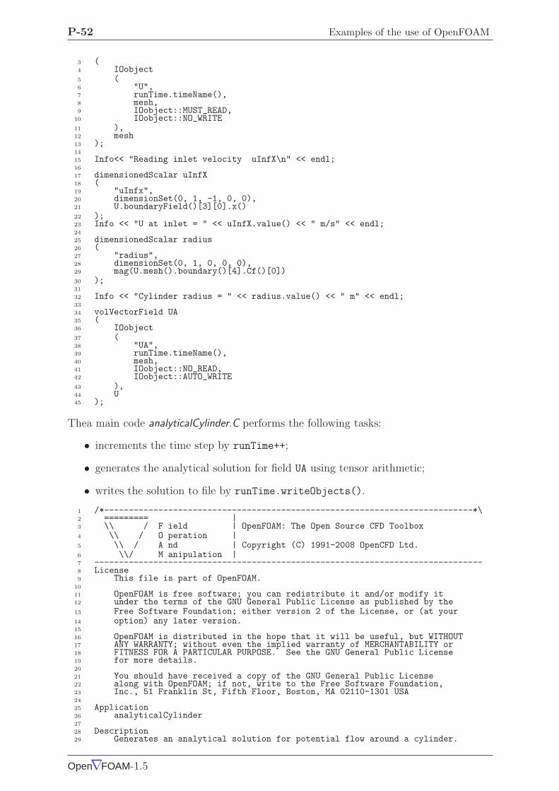
P-52 Examples of the use of OpenFOAM
3 (4 IOobject5 (6 "U",7 runTime.timeName(),8 mesh,9 IOobject::MUST_READ,
10 IOobject::NO_WRITE11 ),12 mesh13 );14
15 Info<< "Reading inlet velocity uInfX\n" << endl;16
17 dimensionedScalar uInfX18 (19 "uInfx",20 dimensionSet(0, 1, -1, 0, 0),21 U.boundaryField()[3][0].x()22 );23 Info << "U at inlet = " << uInfX.value() << " m/s" << endl;24
25 dimensionedScalar radius26 (27 "radius",28 dimensionSet(0, 1, 0, 0, 0),29 mag(U.mesh().boundary()[4].Cf()[0])30 );31
32 Info << "Cylinder radius = " << radius.value() << " m" << endl;33
34 volVectorField UA35 (36 IOobject37 (38 "UA",39 runTime.timeName(),40 mesh,41 IOobject::NO_READ,42 IOobject::AUTO_WRITE43 ),44 U45 );
Thea main code analyticalCylinder.C performs the following tasks:
• increments the time step by runTime++;
• generates the analytical solution for field UA using tensor arithmetic;
• writes the solution to file by runTime.writeObjects().
1 /*---------------------------------------------------------------------------*\2 ========= |3 \\ / F ield | OpenFOAM: The Open Source CFD Toolbox4 \\ / O peration |5 \\ / A nd | Copyright (C) 1991-2008 OpenCFD Ltd.6 \\/ M anipulation |7 -------------------------------------------------------------------------------8 License9 This file is part of OpenFOAM.
10
11 OpenFOAM is free software; you can redistribute it and/or modify it12 under the terms of the GNU General Public License as published by the13 Free Software Foundation; either version 2 of the License, or (at your14 option) any later version.15
16 OpenFOAM is distributed in the hope that it will be useful, but WITHOUT17 ANY WARRANTY; without even the implied warranty of MERCHANTABILITY or18 FITNESS FOR A PARTICULAR PURPOSE. See the GNU General Public License19 for more details.20
21 You should have received a copy of the GNU General Public License22 along with OpenFOAM; if not, write to the Free Software Foundation,23 Inc., 51 Franklin St, Fifth Floor, Boston, MA 02110-1301 USA24
25 Application26 analyticalCylinder27
28 Description29 Generates an analytical solution for potential flow around a cylinder.
Open∇FOAM-1.5

3.2 Steady turbulent flow over a backward-facing step P-53
30 Can be compared with the solution from the potentialFlow/cylinder example.31
32 \*---------------------------------------------------------------------------*/33
34 #include "fvCFD.H"35
36
37 // * * * * * * * * * * * * * * * * * * * * * * * * * * * * * * * * * * * * * //38
39 int main(int argc, char *argv[])40 41
42 # include "setRootCase.H"43
44 # include "createTime.H"45 # include "createMesh.H"46 # include "createFields.H"47
48 // * * * * * * * * * * * * * * * * * * * * * * * * * * * * * * * * * * * * * //49
50 Info << "\nEvaluating analytical solution" << endl;51
52 volVectorField centres = UA.mesh().C();53 volScalarField magCentres = mag(centres);54 volScalarField theta = acos((centres & vector(1,0,0))/magCentres);55
56 volVectorField cs2theta =57 cos(2*theta)*vector(1,0,0)58 + sin(2*theta)*vector(0,1,0);59
60 UA = uInfX*(dimensionedVector(vector(1,0,0))61 - pow((radius/magCentres),2)*cs2theta);62
63 runTime.write();64
65 Info<< "end" << endl;66
67 return(0);68 69
70 // ************************************************************************* //
The utility must be compiled with wmake as normal. It can then be run by typing
analyticalCylinder $FOAM RUN/potentialFoam cylinder
The analytical solution is plotted as streamlines as shown in Figure 3.3(c). Note thatdifferences in the analytical and numerical solutions at the top plane are due to the factthat the analytical solution assumes an infinite boundary and the numerical solutionspecifies a zeroGradient boundary condition at that boundary.
3.1.7 Exercise
Investigate the accuracy of the numerical solution by implementing some measure ofcomparison between the numercial and analytical in analyticalCylinder.
3.2 Steady turbulent flow over a backward-facing step
In this example we shall investigate steady turbulent flow over a backward-facing step.The problem description is taken from one used by Pitz and Daily in an experimentalinvestigation [**] against which the computed solution can be compared. This exampleintroduces the following OpenFOAM features for the first time:
• generation of a mesh using blockMesh using full mesh grading capability;
• steady turbulent flow.
Open∇FOAM-1.5

P-54 Examples of the use of OpenFOAM
3.2.1 Problem specification
The problem is defined as follows:
Solution domain The domain is 2 dimensional, consisting of a short inlet, a backward-facing step and converging nozzle at outlet as shown in Figure 3.4.
84.020.6 206.0
Inlet: Ux = 10.0 m/s Outlet: p = 0 Pa
50.8 33.2
y
x
Dimensions in mm
Figure 3.4: Geometry of backward-facing step
Governing equations
• Mass continuity for incompressible flow
∇ •U = 0 (3.4)
• Steady flow momentum equation
∇ • (UU) + ∇ •R = −∇p (3.5)
where p is kinematic pressure and (in slightly over-simplistic terms) R =νeff∇U is the viscous stress term with an effective kinematic viscosity νeff ,calculated from selected transport and turbulence models.
Initial conditions U = 0 m/s, p = 0 Pa — required in OpenFOAM input files but notnecessary for the solution since the problem is steady-state.
Boundary conditions
• Inlet (left) with fixed velocity U = (10, 0, 0) m/s;
• Outlet (right) with fixed pressure p = 0 Pa;
• No-slip walls on other boundaries.
Transport properties
• Kinematic viscosity of air ν = µ/ρ = 18.1 × 10⁻⁶/1.293 = 14.0 µm2/s
Turbulence model
• Standard k − ǫ;
• Coefficients: Cµ = 0.09; C1 = 1.44; C2 = 1.92; αk = 1; αǫ = 0.76923.
Solver name simpleFoam: an implementation for steady incompressible flow.
Open∇FOAM-1.5

3.2 Steady turbulent flow over a backward-facing step P-55
Case name pitzDaily, located in the $FOAM TUTORIALS/simpleFoam directory.
The problem is solved using simpleFoam, so-called as it is an implementation for steadyflow using the SIMPLE algorithm [**]. The solver has full access to all the turbulencemodels in the incompressibleTurbulenceModels library and the non-Newtonian models in-compressibleTransportModels library of the standard OpenFOAM release.
3.2.2 Mesh generation
We expect that the flow in this problem is reasonably complex and an optimum solutionwill require grading of the mesh. In general, the regions of highest shear are particularlycritical, requiring a finer mesh than in the regions of low shear. We can anticipatewhere high shear will occur by considering what the solution might be in advance of anycalculation. At the inlet we have strong uniform flow in the x direction and, as it passesover the step, it generates shear on the fluid below, generating a vortex in the bottomhalf of the domain. The regions of high shear will therefore be close to the centreline ofthe domain and close to the walls.
The domain is subdivided into 12 blocks as shown in Figure 3.5.
1
14
13
12
11
3
7
82
1
5
4 10
2
3
4
6
7
8
9
11
0 5
10
16
17
1920
21
18
9 15
12
upperWall
outlet0 6
inlet
lowerWall
Figure 3.5: Blocks in backward-facing step
The mesh is 3 dimensional, as always in OpenFOAM, so in Figure 3.5 we are viewingthe back plane along z = −0.5. The full set of vertices and blocks are given in the meshdescription file below:
1 /*--------------------------------*- C++ -*----------------------------------*\2 | ========= | |3 | \\ / F ield | OpenFOAM: The Open Source CFD Toolbox |4 | \\ / O peration | Version: 1.5 |5 | \\ / A nd | Web: http://www.OpenFOAM.org |6 | \\/ M anipulation | |7 \*---------------------------------------------------------------------------*/8 FoamFile9
10 version 2.0;11 format ascii;12 class dictionary;13 object blockMeshDict;14 15 // * * * * * * * * * * * * * * * * * * * * * * * * * * * * * * * * * * * * * //16
17 convertToMeters 0.001;18
19 vertices20 (21 (-20.6 0 -0.5)22 (-20.6 3 -0.5)23 (-20.6 12.7 -0.5)
Open∇FOAM-1.5

P-56 Examples of the use of OpenFOAM
24 (-20.6 25.4 -0.5)25 (0 -25.4 -0.5)26 (0 -5 -0.5)27 (0 0 -0.5)28 (0 3 -0.5)29 (0 12.7 -0.5)30 (0 25.4 -0.5)31 (206 -25.4 -0.5)32 (206 -8.5 -0.5)33 (206 0 -0.5)34 (206 6.5 -0.5)35 (206 17 -0.5)36 (206 25.4 -0.5)37 (290 -16.6 -0.5)38 (290 -6.3 -0.5)39 (290 0 -0.5)40 (290 4.5 -0.5)41 (290 11 -0.5)42 (290 16.6 -0.5)43 (-20.6 0 0.5)44 (-20.6 3 0.5)45 (-20.6 12.7 0.5)46 (-20.6 25.4 0.5)47 (0 -25.4 0.5)48 (0 -5 0.5)49 (0 0 0.5)50 (0 3 0.5)51 (0 12.7 0.5)52 (0 25.4 0.5)53 (206 -25.4 0.5)54 (206 -8.5 0.5)55 (206 0 0.5)56 (206 6.5 0.5)57 (206 17 0.5)58 (206 25.4 0.5)59 (290 -16.6 0.5)60 (290 -6.3 0.5)61 (290 0 0.5)62 (290 4.5 0.5)63 (290 11 0.5)64 (290 16.6 0.5)65 );66
67 blocks68 (69 hex (0 6 7 1 22 28 29 23) (18 7 1) simpleGrading (0.5 1.8 1)70 hex (1 7 8 2 23 29 30 24) (18 10 1) simpleGrading (0.5 4 1)71 hex (2 8 9 3 24 30 31 25) (18 13 1) simpleGrading (0.5 0.25 1)72 hex (4 10 11 5 26 32 33 27) (180 18 1) simpleGrading (4 1 1)73 hex (5 11 12 6 27 33 34 28) (180 9 1) edgeGrading (4 4 4 4 0.5 1 1 0.5 1 1 1 1)74 hex (6 12 13 7 28 34 35 29) (180 7 1) edgeGrading (4 4 4 4 1.8 1 1 1.8 1 1 1 1)75 hex (7 13 14 8 29 35 36 30) (180 10 1) edgeGrading (4 4 4 4 4 1 1 4 1 1 1 1)76 hex (8 14 15 9 30 36 37 31) (180 13 1) simpleGrading (4 0.25 1)77 hex (10 16 17 11 32 38 39 33) (25 18 1) simpleGrading (2.5 1 1)78 hex (11 17 18 12 33 39 40 34) (25 9 1) simpleGrading (2.5 1 1)79 hex (12 18 19 13 34 40 41 35) (25 7 1) simpleGrading (2.5 1 1)80 hex (13 19 20 14 35 41 42 36) (25 10 1) simpleGrading (2.5 1 1)81 hex (14 20 21 15 36 42 43 37) (25 13 1) simpleGrading (2.5 0.25 1)82 );83
84 edges85 (86 );87
88 patches89 (90 patch inlet91 (92 (0 22 23 1)93 (1 23 24 2)94 (2 24 25 3)95 )96 patch outlet97 (98 (16 17 39 38)99 (17 18 40 39)
100 (18 19 41 40)101 (19 20 42 41)102 (20 21 43 42)103 )104 wall upperWall105 (106 (3 25 31 9)
Open∇FOAM-1.5
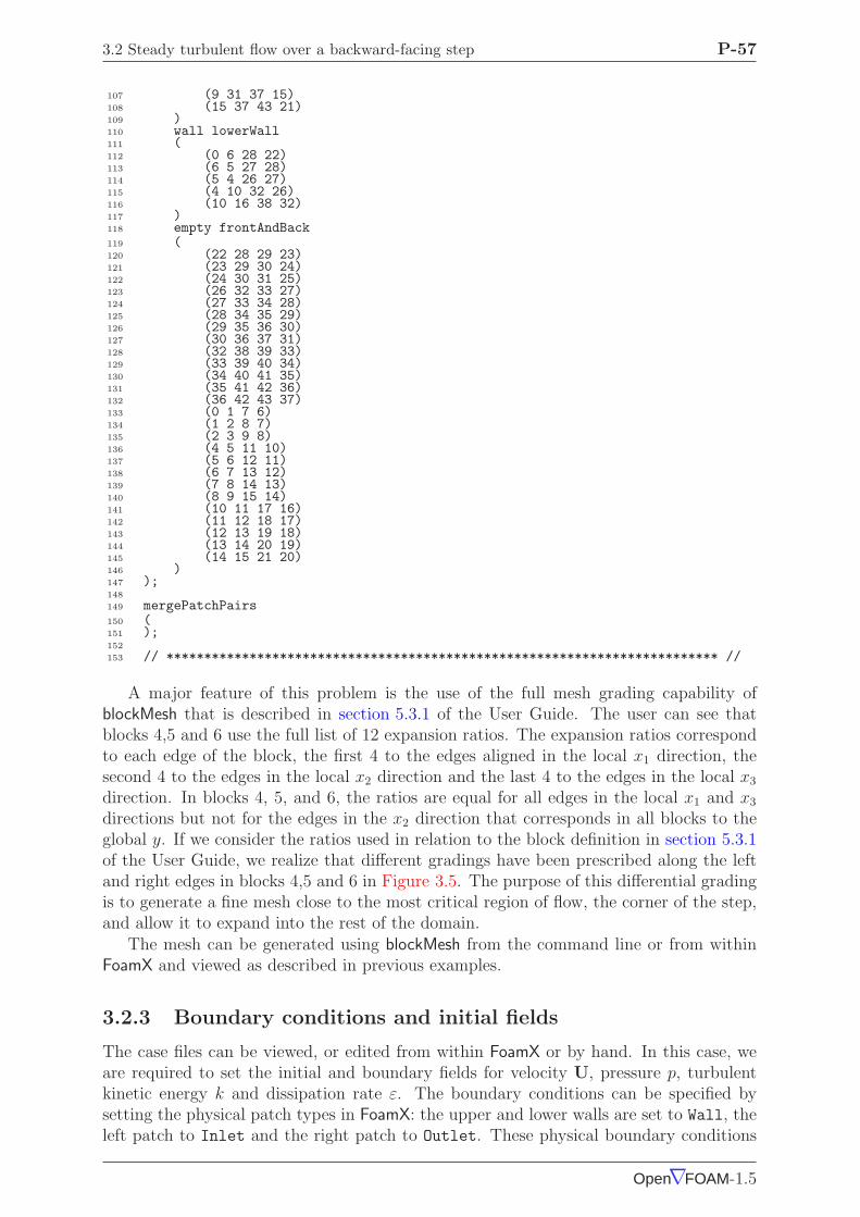
3.2 Steady turbulent flow over a backward-facing step P-57
107 (9 31 37 15)108 (15 37 43 21)109 )110 wall lowerWall111 (112 (0 6 28 22)113 (6 5 27 28)114 (5 4 26 27)115 (4 10 32 26)116 (10 16 38 32)117 )118 empty frontAndBack119 (120 (22 28 29 23)121 (23 29 30 24)122 (24 30 31 25)123 (26 32 33 27)124 (27 33 34 28)125 (28 34 35 29)126 (29 35 36 30)127 (30 36 37 31)128 (32 38 39 33)129 (33 39 40 34)130 (34 40 41 35)131 (35 41 42 36)132 (36 42 43 37)133 (0 1 7 6)134 (1 2 8 7)135 (2 3 9 8)136 (4 5 11 10)137 (5 6 12 11)138 (6 7 13 12)139 (7 8 14 13)140 (8 9 15 14)141 (10 11 17 16)142 (11 12 18 17)143 (12 13 19 18)144 (13 14 20 19)145 (14 15 21 20)146 )147 );148
149 mergePatchPairs150 (151 );152
153 // ************************************************************************* //
A major feature of this problem is the use of the full mesh grading capability ofblockMesh that is described in section 5.3.1 of the User Guide. The user can see thatblocks 4,5 and 6 use the full list of 12 expansion ratios. The expansion ratios correspondto each edge of the block, the first 4 to the edges aligned in the local x1 direction, thesecond 4 to the edges in the local x2 direction and the last 4 to the edges in the local x3
direction. In blocks 4, 5, and 6, the ratios are equal for all edges in the local x1 and x3
directions but not for the edges in the x2 direction that corresponds in all blocks to theglobal y. If we consider the ratios used in relation to the block definition in section 5.3.1of the User Guide, we realize that different gradings have been prescribed along the leftand right edges in blocks 4,5 and 6 in Figure 3.5. The purpose of this differential gradingis to generate a fine mesh close to the most critical region of flow, the corner of the step,and allow it to expand into the rest of the domain.
The mesh can be generated using blockMesh from the command line or from withinFoamX and viewed as described in previous examples.
3.2.3 Boundary conditions and initial fields
The case files can be viewed, or edited from within FoamX or by hand. In this case, weare required to set the initial and boundary fields for velocity U, pressure p, turbulentkinetic energy k and dissipation rate ε. The boundary conditions can be specified bysetting the physical patch types in FoamX: the upper and lower walls are set to Wall, theleft patch to Inlet and the right patch to Outlet. These physical boundary conditions
Open∇FOAM-1.5
P-58 Examples of the use of OpenFOAM
require us to specify a fixedValue at the inlet on U, k and ε. U is given in the problemspecification, but the values of k and ǫ must be chosen by the user in a similar manner tothat described in section 2.1.8.1 of the User Guide. We assume that the inlet turbulenceis isotropic and estimate the fluctuations to be 5% of U at the inlet. We have
U ′
x = U ′
y = U ′
z =5
10010 = 0.5 m/s (3.6)
and
k =3
2(0.5)2 = 0.375 m2/s2 (3.7)
If we estimate the turbulent length scale l to be 10% of the width of the inlet then
ε =C0.75
µ k1.5
l=
0.090.750.3751.5
0.1 × 25.4 × 10−3= 14.855 m2/s3 (3.8)
At the outlet we need only specify the pressure p = 0Pa.
3.2.4 Case control
The choices of fvSchemes are as follows: the timeScheme should be SteadyState; thegradScheme and laplacianScheme should be set as default to Gauss; and, the divSchemeshould be set to UD to ensure boundedness.
Special attention should be paid to the settings of fvTolerances. Although the toplevel simpleFoam code contains only equations for p and U, the turbulent model solvesequations for k, ε and R, and tolerance settings are required for all 5 equations. AsolverTolerance of 10−5 and solverRelativeTolerance of 0.1 are acceptable for allvariables with the exception of p when 10−6 and 0.01 are recommended. Under-relaxationof the solution is required since the problem is steady. A relaxationFactor of 0.7 isacceptable for U, k, ε and R but 0.3 is required for p to avoid numerical instability.
Finally, in controlDict, the time step deltaT should be set to 1 since in steady statecases such as this is effectively an iteration counter. With benefit of hindsight we knowthat the solution requires 1000 iterations reach reasonable convergence, hence endTime isset to 1000. Ensure that the writeFrequency is sufficiently high, e.g. 50, that you willnot fill the hard disk with data during run time.
3.2.5 Running the case and post-processing
Run the case and post-process the results. After a few iterations, e.g. 50, a vortex developsbeneath the corner of the step that is the height of the step but narrow in the x-directionas shown by the vector plot of velocities is shown Figure 3.6(a). Over several iterationsthe vortex stretches in the x-direction from the step to the outlet until at 1000 iterationsthe system reaches a steady-state in which the vortex is fully developed as shown inFigure 3.6(b-c).
3.3 Supersonic flow over a forward-facing step
In this example we shall investigate supersonic flow over a forward-facing step. Theproblem description involves a flow of Mach 3 at an inlet to a rectangular geometry witha step near the inlet region that generates shock waves.
This example introduces the following OpenFOAM features for the first time:
• supersonic flow;
Open∇FOAM-1.5

3.3 Supersonic flow over a forward-facing step P-59
(a) Velocity vectors after 50 iterations
(b) Velocity vectors at 1000 iterations
(c) Streamlines at 1000 iterations
Figure 3.6: Development of a vortex in the backward-facing step.
3.3.1 Problem specification
The problem is defined as follows:
Solution domain The domain is 2 dimensional and consists of a short inlet sectionfollowed by a forward-facing step of 20% the height of the section as shown inFigure 3.7
y0.2
Inlet: Ux = Mach 3, p = 1 N/m2
x
1.0
0.6 2.4Dimensions in m
Figure 3.7: Geometry of the forward step geometry
Governing equations
• Mass continuity
∂ρ
∂t+ ∇ • (ρU) = 0 (3.9)
• Ideal gas
p = ρRT (3.10)
Open∇FOAM-1.5

P-60 Examples of the use of OpenFOAM
• Momentum equation for Newtonian fluid
∂ρU
∂t+ ∇ • (ρUU) −∇ • µ∇U = −∇p (3.11)
• Energy equation for fluid (ignoring some viscous terms), e = CvT , with Fourier’sLaw q = −k∇T
∂ρe
∂t+ ∇ • (ρUe) −∇ •
(k
Cv
)
∇e = p∇ •U (3.12)
Initial conditions U = 0 m/s, p = 1 Pa, T = 1 K.
Boundary conditions
• Inlet (left) with fixedValue for velocity U = 3 m/s = Mach 3, pressure p = 1 Paand temperature T = 1 K;
• Outlet (right) with zeroGradient on U , p and T ;
• No-slip adiabatic wall (bottom);
• Symmetry plane (top).
Transport properties
• Dynamic viscosity of air µ = 18.1µPa s
Thermodynamic properties
• Specific heat at constant volume Cv = 1.78571 J/kg K
• Gas constant R = 0.714286 J/kg K
• Conductivity k = 32.3 µW/m K
Case name forwardStep case located in the $FOAM TUTORIALS/sonicFoam directory.
Solver name sonicFoam: an implementation for compressible trans-sonic/supersoniclaminar gas flow.
The case is designed such that the speed of sound of the gas c =√
γRT = 1 m/s, theconsequence being that the velocities are directly equivalent to the Mach number, e.g.
the inlet velocity of 3 m/s is equivalent to Mach 3. This speed of sound calculation canbe verified using the relationship for a perfect gas, Cp −Cv = R, i.e. the ratio of specificheats
γ = Cp/Cv =R
Cv
+ 1 (3.13)
3.3.2 Mesh generation
The mesh used in this case is relatively simple, specified with uniform rectangular cellsof length 0.06 m in the x direction and 0.05 m in the y direction. The geometry cansimply be divided into 3 blocks, one below the top of the step, and two above the step,one either side of the step front. The full set of vertices and blocks are given in the meshdescription file below:
Open∇FOAM-1.5
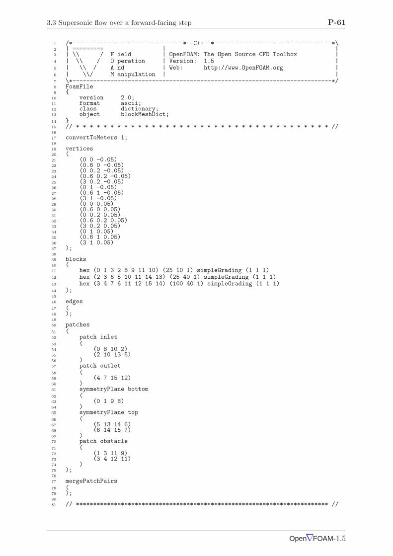
3.3 Supersonic flow over a forward-facing step P-61
1 /*--------------------------------*- C++ -*----------------------------------*\2 | ========= | |3 | \\ / F ield | OpenFOAM: The Open Source CFD Toolbox |4 | \\ / O peration | Version: 1.5 |5 | \\ / A nd | Web: http://www.OpenFOAM.org |6 | \\/ M anipulation | |7 \*---------------------------------------------------------------------------*/8 FoamFile9
10 version 2.0;11 format ascii;12 class dictionary;13 object blockMeshDict;14 15 // * * * * * * * * * * * * * * * * * * * * * * * * * * * * * * * * * * * * * //16
17 convertToMeters 1;18
19 vertices20 (21 (0 0 -0.05)22 (0.6 0 -0.05)23 (0 0.2 -0.05)24 (0.6 0.2 -0.05)25 (3 0.2 -0.05)26 (0 1 -0.05)27 (0.6 1 -0.05)28 (3 1 -0.05)29 (0 0 0.05)30 (0.6 0 0.05)31 (0 0.2 0.05)32 (0.6 0.2 0.05)33 (3 0.2 0.05)34 (0 1 0.05)35 (0.6 1 0.05)36 (3 1 0.05)37 );38
39 blocks40 (41 hex (0 1 3 2 8 9 11 10) (25 10 1) simpleGrading (1 1 1)42 hex (2 3 6 5 10 11 14 13) (25 40 1) simpleGrading (1 1 1)43 hex (3 4 7 6 11 12 15 14) (100 40 1) simpleGrading (1 1 1)44 );45
46 edges47 (48 );49
50 patches51 (52 patch inlet53 (54 (0 8 10 2)55 (2 10 13 5)56 )57 patch outlet58 (59 (4 7 15 12)60 )61 symmetryPlane bottom62 (63 (0 1 9 8)64 )65 symmetryPlane top66 (67 (5 13 14 6)68 (6 14 15 7)69 )70 patch obstacle71 (72 (1 3 11 9)73 (3 4 12 11)74 )75 );76
77 mergePatchPairs78 (79 );80
81 // ************************************************************************* //
Open∇FOAM-1.5

P-62 Examples of the use of OpenFOAM
3.3.3 Running the case
The case approaches a steady-state at some time after 5 s. The results for pressure at10 s are shown in Figure 3.8. The results clearly show discontinuities in pressure, i.e.
shock waves, emanating from ahead of the base of the step.
6
8
10
12
4
2
14
pressureShock fronts
Figure 3.8: Shock fronts in the forward step problem
3.3.4 Exercise
The user can examine the effect on the solution of increasing the inlet velocity.
3.4 Decompression of a tank internally pressurised
with water
In this example we shall investigate a problem of rapid opening of a pipe valve close toa pressurised liquid-filled tank. The prominent feature of the result in such cases is thepropagation of pressure waves which must therefore be modelled as a compressible liquid.
This tutorial introduces the following OpenFOAM features for the first time:
• Mesh refinement
• Pressure waves in liquids
3.4.1 Problem specification
Solution domain The domain is 2 dimensional and consists of a tank with a smalloutflow pipe as shown in Figure 3.9
Governing equations This problem requires a model for compressibility ψ in the fluidin order to be able to resolve waves propagating at a finite speed. A barotropicrelationship is used to relate density ρ and pressure p are related to ψ.
• Mass continuity
∂ρ
∂t+ ∇ • (ρU) = 0 (3.14)
Open∇FOAM-1.5

3.4 Decompression of a tank internally pressurised with water P-63
x
y
Outlet: p = 0 bar24050
10
50
100
orientation of horizontal x-axisNote:Dimensions in mm
image is rotated through -90 from normal
Figure 3.9: Geometry of a tank with outflow pipe
• The barotropic relationship
∂ρ
∂p=
ρ
K= ψ (3.15)
where K is the bulk modulus
• Equation 3.15 is linearised as
ρ ≈ ρ0 + ψ (p − p0) (3.16)
where ρ0 and p0 are the reference density and pressure respectively such thatρ(p0) = ρ0.
• Momentum equation for Newtonian fluid
∂ρU
∂t+ ∇ • (ρUU) −∇ • µ∇U = −∇p (3.17)
Boundary conditions Using FoamX the following physical boundary conditions canbe set:
• outerWall is specified the wall condition;
• axis is specified as the symmetryPlane;
• nozzle is specified as a pressureOutlet where p = 0 bar.
• front and back boundaries are specified as empty.
Initial conditions U = 0 m/s, p = 100 bar.
Transport properties
• Dynamic viscosity of water µ = 1.0 mPa s
Thermodynamic properties
• Density of water ρ = 1000 kg/m3
• Reference pressure p0 = 1 bar
• Compressibility of water ψ = 4.54 × 10⁻⁷ s2/m2
Solver name sonicLiquidFoam: a compressible sonic laminar liquid flow code.
Case name decompressionTank case located in the $FOAM TUTORIALS/sonicLiquidFoamdirectory.
Open∇FOAM-1.5

P-64 Examples of the use of OpenFOAM
3.4.2 Mesh Generation
The full geometry is modelled in this case; the set of vertices and blocks are given in themesh description file below:
1 /*--------------------------------*- C++ -*----------------------------------*\2 | ========= | |3 | \\ / F ield | OpenFOAM: The Open Source CFD Toolbox |4 | \\ / O peration | Version: 1.5 |5 | \\ / A nd | Web: http://www.OpenFOAM.org |6 | \\/ M anipulation | |7 \*---------------------------------------------------------------------------*/8 FoamFile9
10 version 2.0;11 format ascii;12 class dictionary;13 object blockMeshDict;14 15 // * * * * * * * * * * * * * * * * * * * * * * * * * * * * * * * * * * * * * //16
17 convertToMeters 0.1;18
19 vertices20 (21 (0 0 -0.1)22 (1 0 -0.1)23 (0 0.5 -0.1)24 (1 0.5 -0.1)25 (1.5 0.5 -0.1)26 (0 0.6 -0.1)27 (1 0.6 -0.1)28 (1.5 0.6 -0.1)29 (0 3 -0.1)30 (1 3 -0.1)31 (0 0 0.1)32 (1 0 0.1)33 (0 0.5 0.1)34 (1 0.5 0.1)35 (1.5 0.5 0.1)36 (0 0.6 0.1)37 (1 0.6 0.1)38 (1.5 0.6 0.1)39 (0 3 0.1)40 (1 3 0.1)41 );42
43 blocks44 (45 hex (0 1 3 2 10 11 13 12) (30 20 1) simpleGrading (1 1 1)46 hex (2 3 6 5 12 13 16 15) (30 5 1) simpleGrading (1 1 1)47 hex (3 4 7 6 13 14 17 16) (25 5 1) simpleGrading (1 1 1)48 hex (5 6 9 8 15 16 19 18) (30 95 1) simpleGrading (1 1 1)49 );50
51 edges52 (53 );54
55 patches56 (57 wall outerWall58 (59 (0 1 11 10)60 (1 3 13 11)61 (3 4 14 13)62 (7 6 16 17)63 (6 9 19 16)64 (9 8 18 19)65 )66 symmetryPlane axis67 (68 (0 10 12 2)69 (2 12 15 5)70 (5 15 18 8)71 )72 patch nozzle73 (74 (4 7 17 14)75 )76 empty back77 (
Open∇FOAM-1.5
3.4 Decompression of a tank internally pressurised with water P-65
78 (0 2 3 1)79 (2 5 6 3)80 (3 6 7 4)81 (5 8 9 6)82 )83 empty front84 (85 (10 11 13 12)86 (12 13 16 15)87 (13 14 17 16)88 (15 16 19 18)89 )90 );91
92 mergePatchPairs93 (94 );95
96 // ************************************************************************* //
In order to improve the numerical accuracy, we shall use the reference level of 1 bar forthe pressure field. Note that both the internal field level and the boundary conditions areoffset by the reference level.
3.4.3 Preparing the Run
Before we commence the setup of the calculation, we need to consider the characteristicvelocity of the phenomenon we are trying to capture. In the case under consideration,the fluid velocity will be very small, but the pressure wave will propagate with the speedof sound in water. The speed of sound is calculated as:
c =
√1
ψ=
√
1
4.54 × 10−7= 1483.2m/s. (3.18)
For the mesh described above, the characteristic mesh size is approximately 2 mm (notethe scaling factor of 0.1 in the blockMeshDict file). Using
Co =U ∆t
∆x(3.19)
a reasonable time step is around ∆t = 5× 10⁻⁷s, giving the Co number of 0.35, based onthe speed of sound. Also, note that the reported Co number by the code (associated withthe convective velocity) will be two orders of magnitude smaller. As we are interested inthe pressure wave propagation, we shall set the simulation time to 0.25 ms. For reference,the controlDict file is quoted below.
1 /*--------------------------------*- C++ -*----------------------------------*\2 | ========= | |3 | \\ / F ield | OpenFOAM: The Open Source CFD Toolbox |4 | \\ / O peration | Version: 1.5 |5 | \\ / A nd | Web: http://www.OpenFOAM.org |6 | \\/ M anipulation | |7 \*---------------------------------------------------------------------------*/8 FoamFile9
10 version 2.0;11 format ascii;12 class dictionary;13 object controlDict;14 15 // * * * * * * * * * * * * * * * * * * * * * * * * * * * * * * * * * * * * * //16
17 application sonicLiquidFoam;18
19 startFrom startTime;20
21 startTime 0;22
23 stopAt endTime;
Open∇FOAM-1.5
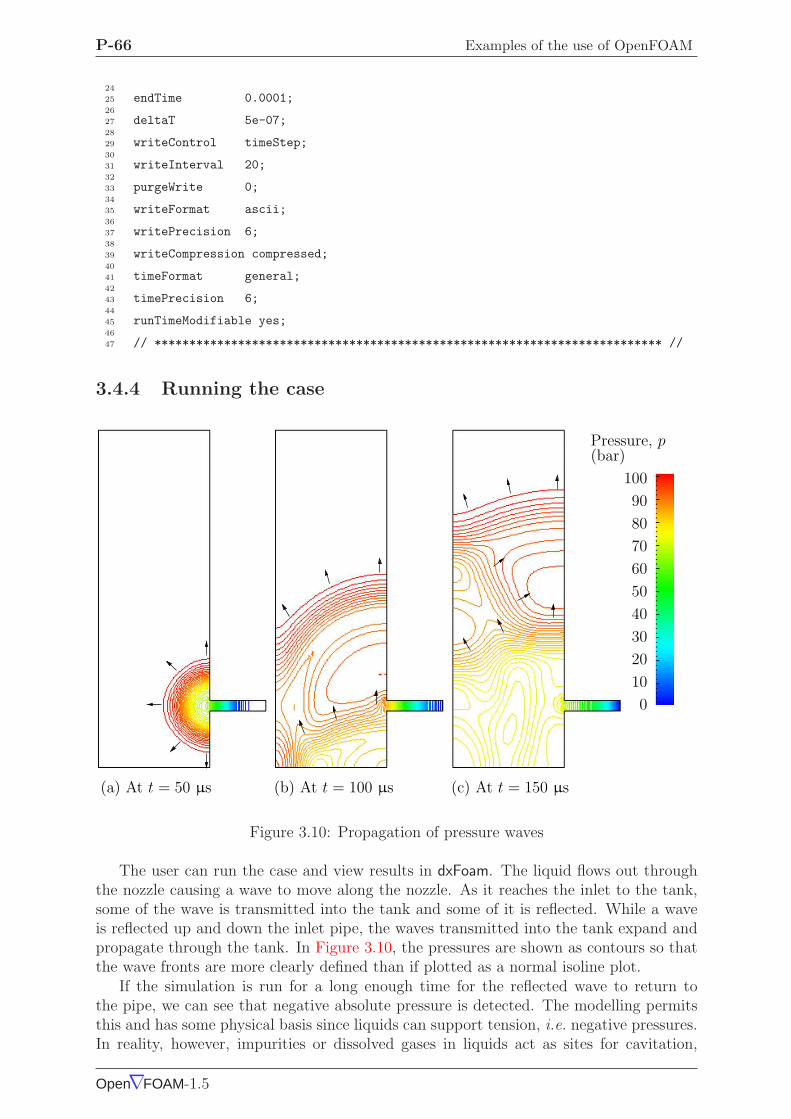
P-66 Examples of the use of OpenFOAM
24
25 endTime 0.0001;26
27 deltaT 5e-07;28
29 writeControl timeStep;30
31 writeInterval 20;32
33 purgeWrite 0;34
35 writeFormat ascii;36
37 writePrecision 6;38
39 writeCompression compressed;40
41 timeFormat general;42
43 timePrecision 6;44
45 runTimeModifiable yes;46
47 // ************************************************************************* //
3.4.4 Running the case
0
10
20
30
40
50
60
70
80
90
100
(a) At t = 50 µs (b) At t = 100 µs (c) At t = 150 µs
Pressure, p(bar)
Figure 3.10: Propagation of pressure waves
The user can run the case and view results in dxFoam. The liquid flows out throughthe nozzle causing a wave to move along the nozzle. As it reaches the inlet to the tank,some of the wave is transmitted into the tank and some of it is reflected. While a waveis reflected up and down the inlet pipe, the waves transmitted into the tank expand andpropagate through the tank. In Figure 3.10, the pressures are shown as contours so thatthe wave fronts are more clearly defined than if plotted as a normal isoline plot.
If the simulation is run for a long enough time for the reflected wave to return tothe pipe, we can see that negative absolute pressure is detected. The modelling permitsthis and has some physical basis since liquids can support tension, i.e. negative pressures.In reality, however, impurities or dissolved gases in liquids act as sites for cavitation,
Open∇FOAM-1.5
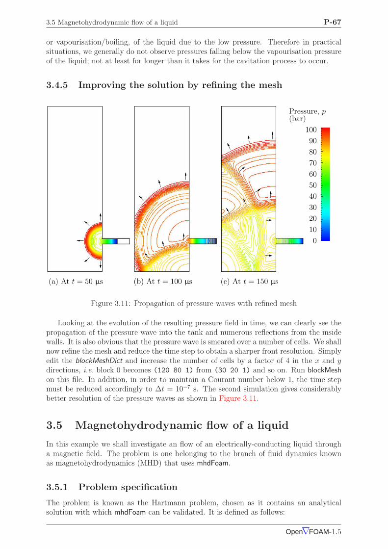
3.5 Magnetohydrodynamic flow of a liquid P-67
or vapourisation/boiling, of the liquid due to the low pressure. Therefore in practicalsituations, we generally do not observe pressures falling below the vapourisation pressureof the liquid; not at least for longer than it takes for the cavitation process to occur.
3.4.5 Improving the solution by refining the mesh
0
10
20
30
40
50
60
70
80
90
100
(a) At t = 50 µs (b) At t = 100 µs (c) At t = 150 µs
Pressure, p(bar)
Figure 3.11: Propagation of pressure waves with refined mesh
Looking at the evolution of the resulting pressure field in time, we can clearly see thepropagation of the pressure wave into the tank and numerous reflections from the insidewalls. It is also obvious that the pressure wave is smeared over a number of cells. We shallnow refine the mesh and reduce the time step to obtain a sharper front resolution. Simplyedit the blockMeshDict and increase the number of cells by a factor of 4 in the x and ydirections, i.e. block 0 becomes (120 80 1) from (30 20 1) and so on. Run blockMeshon this file. In addition, in order to maintain a Courant number below 1, the time stepmust be reduced accordingly to ∆t = 10−7 s. The second simulation gives considerablybetter resolution of the pressure waves as shown in Figure 3.11.
3.5 Magnetohydrodynamic flow of a liquid
In this example we shall investigate an flow of an electrically-conducting liquid througha magnetic field. The problem is one belonging to the branch of fluid dynamics knownas magnetohydrodynamics (MHD) that uses mhdFoam.
3.5.1 Problem specification
The problem is known as the Hartmann problem, chosen as it contains an analyticalsolution with which mhdFoam can be validated. It is defined as follows:
Open∇FOAM-1.5
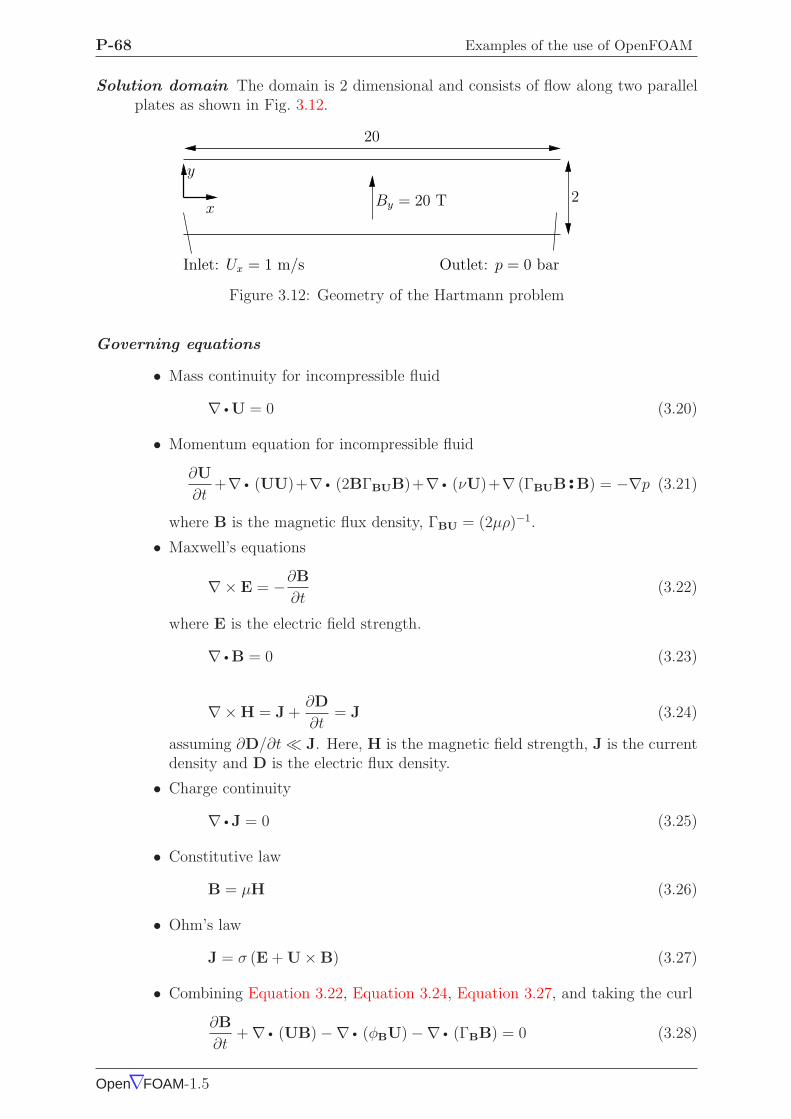
P-68 Examples of the use of OpenFOAM
Solution domain The domain is 2 dimensional and consists of flow along two parallelplates as shown in Fig. 3.12.
y
x2
20
Outlet: p = 0 barInlet: Ux = 1 m/s
By = 20 T
Figure 3.12: Geometry of the Hartmann problem
Governing equations
• Mass continuity for incompressible fluid
∇ •U = 0 (3.20)
• Momentum equation for incompressible fluid
∂U
∂t+∇ • (UU)+∇ • (2BΓBUB)+∇ • (νU)+∇ (ΓBUB •
•B) = −∇p (3.21)
where B is the magnetic flux density, ΓBU = (2µρ)−1.
• Maxwell’s equations
∇× E = −∂B
∂t(3.22)
where E is the electric field strength.
∇ •B = 0 (3.23)
∇× H = J +∂D
∂t= J (3.24)
assuming ∂D/∂t ≪ J. Here, H is the magnetic field strength, J is the currentdensity and D is the electric flux density.
• Charge continuity
∇ •J = 0 (3.25)
• Constitutive law
B = µH (3.26)
• Ohm’s law
J = σ (E + U × B) (3.27)
• Combining Equation 3.22, Equation 3.24, Equation 3.27, and taking the curl
∂B
∂t+ ∇ • (UB) −∇ • (φBU) −∇ • (ΓBB) = 0 (3.28)
Open∇FOAM-1.5
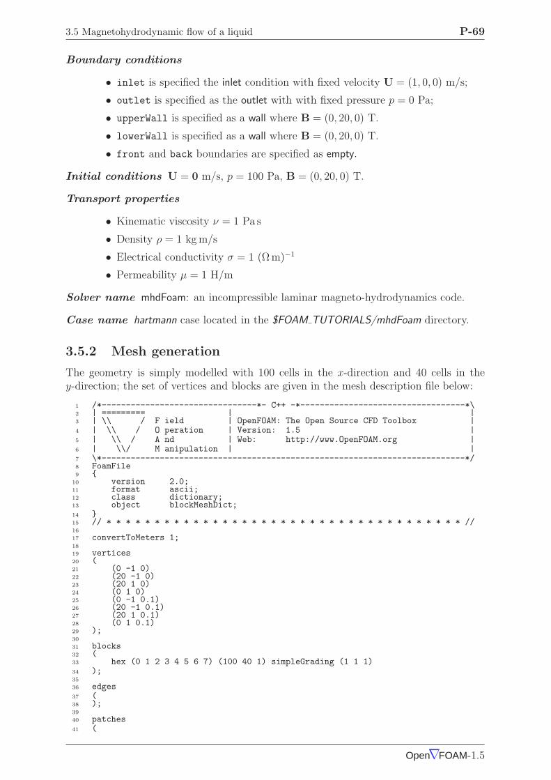
3.5 Magnetohydrodynamic flow of a liquid P-69
Boundary conditions
• inlet is specified the inlet condition with fixed velocity U = (1, 0, 0) m/s;
• outlet is specified as the outlet with with fixed pressure p = 0 Pa;
• upperWall is specified as a wall where B = (0, 20, 0) T.
• lowerWall is specified as a wall where B = (0, 20, 0) T.
• front and back boundaries are specified as empty.
Initial conditions U = 0 m/s, p = 100 Pa, B = (0, 20, 0) T.
Transport properties
• Kinematic viscosity ν = 1 Pa s
• Density ρ = 1 kg m/s
• Electrical conductivity σ = 1 (Ω m)−1
• Permeability µ = 1 H/m
Solver name mhdFoam: an incompressible laminar magneto-hydrodynamics code.
Case name hartmann case located in the $FOAM TUTORIALS/mhdFoam directory.
3.5.2 Mesh generation
The geometry is simply modelled with 100 cells in the x-direction and 40 cells in they-direction; the set of vertices and blocks are given in the mesh description file below:
1 /*--------------------------------*- C++ -*----------------------------------*\2 | ========= | |3 | \\ / F ield | OpenFOAM: The Open Source CFD Toolbox |4 | \\ / O peration | Version: 1.5 |5 | \\ / A nd | Web: http://www.OpenFOAM.org |6 | \\/ M anipulation | |7 \*---------------------------------------------------------------------------*/8 FoamFile9
10 version 2.0;11 format ascii;12 class dictionary;13 object blockMeshDict;14 15 // * * * * * * * * * * * * * * * * * * * * * * * * * * * * * * * * * * * * * //16
17 convertToMeters 1;18
19 vertices20 (21 (0 -1 0)22 (20 -1 0)23 (20 1 0)24 (0 1 0)25 (0 -1 0.1)26 (20 -1 0.1)27 (20 1 0.1)28 (0 1 0.1)29 );30
31 blocks32 (33 hex (0 1 2 3 4 5 6 7) (100 40 1) simpleGrading (1 1 1)34 );35
36 edges37 (38 );39
40 patches41 (
Open∇FOAM-1.5

P-70 Examples of the use of OpenFOAM
42 patch inlet43 (44 (0 4 7 3)45 )46 patch outlet47 (48 (2 6 5 1)49 )50 patch lowerWall51 (52 (1 5 4 0)53 )54 patch upperWall55 (56 (3 7 6 2)57 )58 empty frontAndBack59 (60 (0 3 2 1)61 (4 5 6 7)62 )63 );64
65 mergePatchPairs66 (67 );68
69 // ************************************************************************* //
3.5.3 Running the case
The user can run the case and view results in dxFoam. It is also useful at this stage to runthe Ucomponents utility to convert the U vector field into individual scalar components.MHD flow is governed by, amongst other things, the Hartmann number which is a measureof the ratio of electromagnetic body force to viscous force
M = BL
√σ
ρν(3.29)
where L is the characteristic length scale. In this case with By = 20 T, M = 20 andthe electromagnetic body forces dominate the viscous forces. Consequently with the flowfairly steady at t = 2 s the velocity profile is almost planar, viewed at a cross sectionmidway along the domain x = 10 m. The user can plot a graph of the profile of Ux indxFoam. Now the user should reduce the magnetic flux density B to 1 Tand re-run thecode and Ucomponents. In this case, M = 1 and the electromagnetic body forces no longerdominate. The velocity profile consequently takes on the parabolic form, characteristicof Poiseuille flow as shown in Figure 3.13. To validate the code the analytical solutionfor the velocity profile Ux is superimposed in Figure 3.13, given by:
Ux(y)
Ux(0)=
cosh M − cosh M(y/L)
cosh M − 1(3.30)
where the characteristic length L is half the width of the domain, i.e. 1 m.
Open∇FOAM-1.5
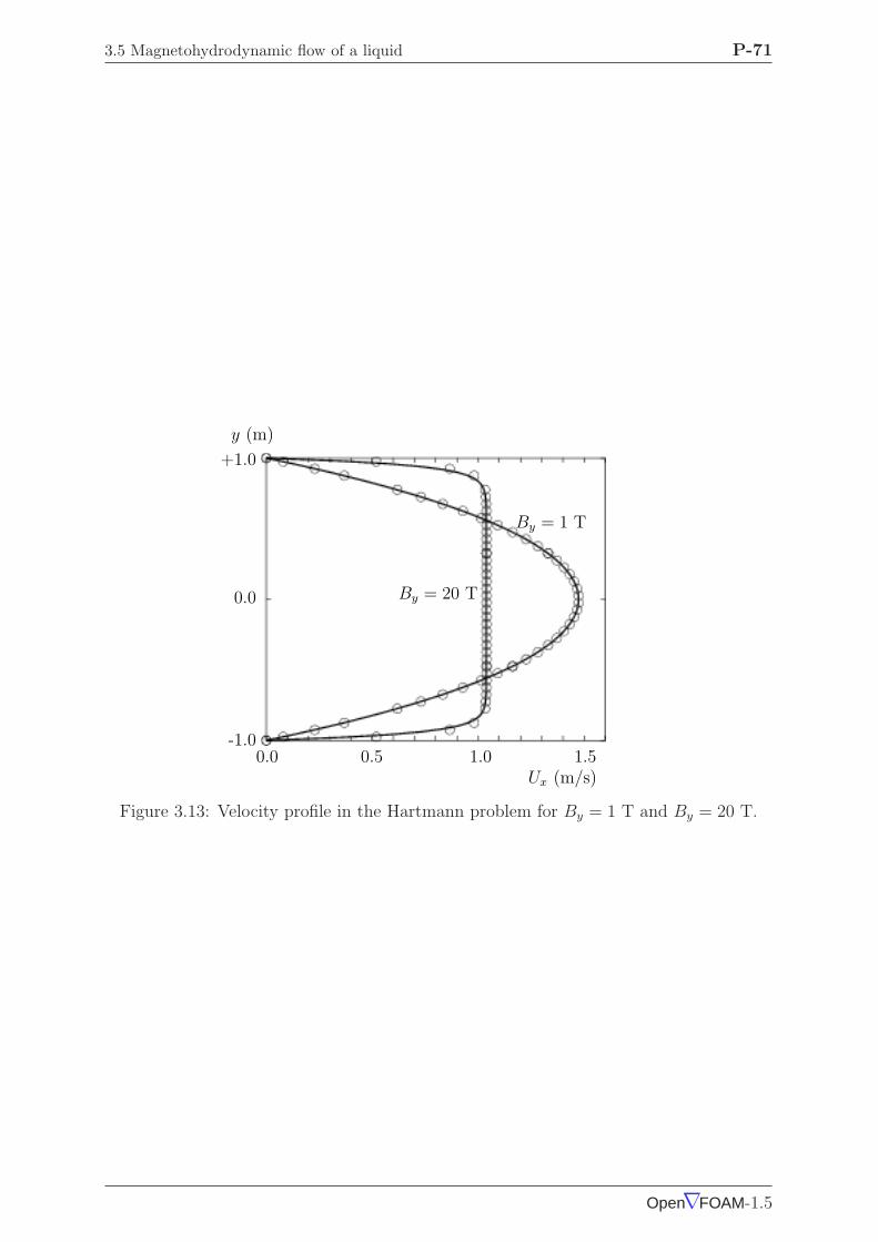
3.5 Magnetohydrodynamic flow of a liquid P-71
0.0 1.0-1.0
0.0
+1.0
y (m)
0.5 1.5
By = 20 T
Ux (m/s)
By = 1 T
Figure 3.13: Velocity profile in the Hartmann problem for By = 1 T and By = 20 T.
Open∇FOAM-1.5

P-72 Examples of the use of OpenFOAM
Open∇FOAM-1.5

Index P-73
Index
Symbols Numbers A B C D E F G H I J K L M N O P Q R S T U V W X Z
Symbols*
tensor member function, P-25+
tensor member function, P-25-
tensor member function, P-25/
tensor member function, P-25/*...*/
C++ syntax, U-76//
C++ syntax, U-76OpenFOAM file syntax, U-98
# include
C++ syntax, U-70, U-76&
tensor member function, P-25&&
tensor member function, P-25^
tensor member function, P-25<LESmodel>Coeffs keyword, U-174<RASModel>Coeffs keyword, U-174<delta>Coeffs keyword, U-1740.000000e+00 directory, U-981-dimensional mesh, U-1221D mesh, U-1222-dimensional mesh, U-1222D mesh, U-122
Numbers0 directory, U-98
Aaccess functions, P-23addLayersControls keyword, U-138adiabaticFlameT utility, U-90adjustableRunTime
keyword entry, U-59, U-105adjustPhi tools, U-91adjustTimeStep keyword, U-59agglomerator keyword, U-115
algorithms tools, U-91
allTime
menu entry, U-184
analytical solution, P-45
anisotropicFilter model, U-94
Annotation window panel, U-25, U-159
ansysToFoam utility, U-86
APIfunctions model, U-93
applications, U-67
Apply button, U-156, U-160
arbitrarily unstructured, P-31
arc
keyword entry, U-132
arc keyword, U-131
ascii
keyword entry, U-105
attachMesh utility, U-87
Auto Accept button, U-159
autoPatch utility, U-87
axes
right-handed, U-130
right-handed rectangular Cartesian, P-15,U-20
axi-symmetric cases, U-127, U-135
axi-symmetric mesh, U-122
Bbackground
process, U-26, U-79
backward
keyword entry, U-112
Backward differencing, P-39
basicThermophysicalModels
library, U-92
binary
keyword entry, U-105
BirdCarreau model, U-95
blended differencing, P-38
block
expansion ratio, U-132
block keyword, U-131
blockMesh solver, P-47
Open∇FOAM-1.5
P-74 Index
blockMesh utility, U-38, U-86, U-127blockMesh executable
vertex numbering, U-132blockMeshDict
dictionary, U-20, U-22, U-36, U-48, U-127,U-136
blocks keyword, U-22, U-32, U-132bound tools, U-91boundaries, U-124boundary, U-124boundary
dictionary, U-121, U-127boundary condition
calculated, U-128cyclic, U-127directionMixed, U-128empty, P-63, P-69, U-20, U-122, U-127fixedGradient, U-128fixedValue, U-128fluxCorrectedVelocity, U-129gammaContactAngle, U-57inlet, P-69inletOutlet, U-129mixed, U-128movingWallVelocity, U-129outlet, P-69outletInlet, U-129partialSlip, U-129patch, U-126pressureDirectedInletVelocity, U-129pressureInletVelocity, U-129pressureOutlet, P-63pressureTransmissive, U-129processor, U-127setup, U-22slip, U-129supersonicFreeStream, U-129surfaceNormalFixedValue, U-129symmetryPlane, P-63, U-126totalPressure, U-129turbulentInlet, U-129wall, U-40wall, P-63, P-69, U-57, U-126wallBuoyantPressure, U-129wedge, U-122, U-127, U-135zeroGradient, U-128
boundary conditions, P-43Dirichlet, P-43inlet, P-44Neumann, P-43no-slip impermeable wall, P-44outlet, P-44physical, P-44symmetry plane, P-44
boundary type
empty, U-187
boundaryField keyword, U-22, U-102
boundaryFoam solver, U-83
bounded
keyword entry, U-110, U-111
boxToCell keyword, U-58
boxTurb utility, U-86
breaking of a dam, U-55
bubbleFoam solver, U-84
buoyantFoam solver, U-85
buoyantSimpleRadiationFoam solver, U-85
buoyantSimpleFoam solver, U-85
button
Apply, U-156, U-160
Auto Accept, U-159
Choose Preset, U-158
Compact, U-187
Delete, U-156
Edit Color Map, U-157
Info, U-187
My Jobs, U-187
Orientation Axes, U-25, U-159
Rescale to Data Range, U-28
Reset, U-156
Set Solid Color, U-158
Update GUI, U-28, U-157
Use Parallel Projection, U-25
Use parallel projection, U-159
cont, U-187
endNow, U-187
end, U-187
kill, U-187
purge, U-187
read, U-187
status, U-187
suspend, U-187
CC++ syntax
/*...*/, U-76
//, U-76
# include, U-70, U-76
cacheAgglomeration keyword, U-115
calculated
boundary condition, U-128
case
browser, U-180
server, U-186
case manager
FoamX (obsolete), U-177
Case Name text box, U-182
Case Root text box, U-182
cases, U-97
Open∇FOAM-1.5
Index P-75
castellatedMesh keyword, U-138castellatedMeshControls
dictionary, U-139, U-141castellatedMeshControls keyword, U-138cavity flow, U-19ccm26ToFoam utility, U-86CEI ARCH
environment variable, U-164CEI HOME
environment variable, U-164cell
expansion ratio, U-132cell class, P-31cell
keyword entry, U-166cellDecompFiniteElement
library, U-91cellPoint
keyword entry, U-166cellPointFace
keyword entry, U-166cells
dictionary, U-127cellSet utility, U-87central differencing, P-38cfdTools
library, U-91cfxToFoam utility, U-86, U-145cGamma keyword, U-61channelOodles solver, U-83Chart Options window, U-35checkMesh utility, U-87, U-146checkYPlus utility, U-89chemistryModel
library, U-93chemistryModel model, U-93chemistrySolver model, U-93chemkinMixture model, U-93, U-172chemkinToFoam utility, U-90Choose Preset button, U-158chtMultiRegionFoam solver, U-85Class menu, U-182class
cell, P-31dimensionSet, P-25, P-32, P-33face, P-31finiteVolumeCalculus, P-33finiteVolumeMethod, P-33fvMesh, P-31fvSchemes, P-36fvc, P-36fvm, P-36pointField, P-31polyBoundaryMesh, P-31
polyMesh, P-31, U-119, U-121polyPatchList, P-31polyPatch, P-31scalarField, P-29scalar, P-23slice, P-31symmTensorField, P-29symmTensorThirdField, P-29tensorField, P-29tensorThirdField, P-29tensor, P-23vectorField, P-29vector, P-23, U-101word, P-25, P-31
class keyword, U-99clockTime
keyword entry, U-105cloud keyword, U-167cmptAv
tensor member function, P-25Co utility, U-88cofactors
tensor member function, P-25coldEngineFoam solver, U-85Color By menu, U-158Color Legend window, U-30Color Legend window panel, U-158Color Scale window panel, U-158combustionThermophysicalModels
library, U-92comments, U-76Compact button, U-187compressed
keyword entry, U-105compressible tools, U-91compressibleLesInterFoam solver, U-84compressibleLESModels
library, U-95compressibleRASModels
library, U-94constant directory, U-98, U-171constLaminarFlameSpeed model, U-93constTransport model, U-93, U-172cont button, U-187containers tools, U-91continuum
mechanics, P-15control
of time, U-104controlDict
dictionary, P-65, U-23, U-32, U-41, U-50,U-59, U-98, U-151
controlDict file, P-49convection, see divergence, P-38
Open∇FOAM-1.5

P-76 Index
convergence, U-39
convertToMeters keyword, U-131
coodles solver, U-84
coordinate
system, P-15
coordinate system, U-20
CORBA, U-92, U-177
corrected
keyword entry, U-110, U-111
couplePatches utility, U-87
Courant number, P-42, U-24
cpuTime
keyword entry, U-105
Crank Nicholson
temporal discretisation, P-42
CrankNicholson
keyword entry, U-112
createPatch utility, U-87
cross product, see tensor, vector cross product
CrossPowerLaw
keyword entry, U-58
CrossPowerLaw model, U-95
cubeRootVolDelta model, U-94
cubicCorrected
keyword entry, U-112
cubicCorrection
keyword entry, U-109
curl, P-37
curl
fvc member function, P-37
Current Time Controls menu, U-28, U-157
curve keyword, U-167
cyclic
boundary condition, U-127
cyclic
keyword entry, U-127
cylinder
flow around a, P-45
Dd2dt2
fvc member function, P-37
fvm member function, P-37
dam
breaking of a, U-55
db tools, U-91
ddt
fvc member function, P-37
fvm member function, P-37
DeardorffDiffStress model, U-95
debug keyword, U-138
decomposePar utility, U-79, U-80, U-90
decomposeParDict
dictionary, U-79
decompositionof field, U-79of mesh, U-79
decompression of a tank, P-62defaultFieldValues keyword, U-58deformedGeom utility, U-87Delete button, U-156delta keyword, U-81, U-174deltaT keyword, U-104dependencies, U-70dependency lists, U-70det
tensor member function, P-25determinant, see tensor, determinantdev
tensor member function, P-25diag
tensor member function, P-25diagonal
keyword entry, U-115DIC
keyword entry, U-115DICGaussSeidel
keyword entry, U-115Dictionaries dictionary tree, U-188dictionary
LESProperties, U-174PISO, U-25RASProperties, U-41, U-174blockMeshDict, U-20, U-22, U-36, U-48,
U-127, U-136boundary, U-121, U-127castellatedMeshControls, U-139, U-141cells, U-127controlDict, P-65, U-23, U-32, U-41, U-50,
U-59, U-98, U-151decomposeParDict, U-79faces, U-121, U-127fvSchemes, U-60, U-98, U-106, U-107fvSolution, U-98, U-113mechanicalProperties, U-49neighbour, U-121owner, U-121points, U-121, U-127thermalProperties, U-50thermophysicalProperties, U-171transportProperties, U-23, U-39, U-41
dictionary treeDictionaries, U-188Fields, U-187
dieselEngineFoam solver, U-85dieselFoam solver, U-85dieselMixture model, U-92, U-172dieselSpray
Open∇FOAM-1.5
Index P-77
library, U-92diEthylEther model, U-93differencing
Backward, P-39blended, P-38central, P-38Euler implicit, P-39Gamma, P-38MINMOD, P-38SUPERBEE, P-38upwind, P-38van Leer, P-38
DILU
keyword entry, U-115dimension
checking in OpenFOAM, P-25, U-101dimensional units, U-101dimensioned<Type> template class, P-25dimensionedTypes tools, U-91dimensions keyword, U-22, U-102dimensionSet class, P-25, P-32, P-33dimensionSet tools, U-91diMethylEther model, U-93direct numerical simulation, U-60directionMixed
boundary condition, U-128directory
0.000000e+00, U-980, U-98Make, U-71constant, U-98, U-171fluentInterface, U-162polyMesh, U-98, U-121processorN , U-80run, U-97system, P-49, U-98tutorials, P-45, U-19
discretisationequation, P-33
Display window panel, U-25, U-28,U-156, U-157
distance
keyword entry, U-141, U-167distributed keyword, U-81, U-82div
fvc member function, P-37fvm member function, P-37
divergence, P-37, P-39divSchemes keyword, U-107divU utility, U-88dnsFoam solver, U-85doLayers keyword, U-138double inner product, see tensor,double inner
product
dx
keyword entry, U-166
dynamicMesh
library, U-91
dynMixedSmagorinsky model, U-94
dynOneEqEddy model, U-94, U-95
dynSmagorinsky model, U-94
EedgeGrading keyword, U-133
edgeMesh
library, U-92
edges keyword, U-131
Edit menu, U-159
Edit Color Map button, U-157
electrostaticFoam solver, U-85
empty
boundary condition, P-63, P-69, U-20,U-122, U-127
empty boundary type, U-187
empty
keyword entry, U-127
end button, U-187
endNow button, U-187
endTime keyword, U-24, U-104
engine
library, U-92
engineCompRatio utility, U-90
engineFoam solver, U-85
engineSwirl utility, U-86
ensight74FoamExec utility, U-164
ensight76FoamExec utility, U-88
ENSIGHT7 INPUT
environment variable, U-164
ENSIGHT7 READER
environment variable, U-164
enstrophy utility, U-88
environment variable
CEI ARCH, U-164
CEI HOME, U-164
ENSIGHT7 INPUT, U-164
ENSIGHT7 READER, U-164
FOAMX PATH, U-192
FOAMX SYSTEM CONFIG, U-192
FOAMX USER CONFIG, U-192
FOAM RUN, U-97, U-192
JAVA HOME, U-192
WM ARCH, U-74
WM COMPILER BIN, U-74
WM COMPILER DIR, U-74
WM COMPILER LIB, U-74
WM COMPILER, U-74
WM COMPILE OPTION, U-74
WM DIR, U-74
Open∇FOAM-1.5
P-78 Index
WM JAVAC OPTION, U-74
WM LINK LANGUAGE, U-74
WM MPLIB, U-74
WM OPTIONS, U-74
WM PROJECT DIR, U-74
WM PROJECT INST DIR, U-74
WM PROJECT LANGUAGE, U-74
WM PROJECT USER DIR, U-74
WM PROJECT VERSION, U-74
WM PROJECT, U-74
WM SHELL, U-74
wmake, U-73
environmentalProperties file, U-58
equilibriumCO utility, U-90
equilibriumFlameT utility, U-90
errorEstimation
library, U-92
errorReduction keyword, U-145
estimateScalarError utility, U-90
Euler
keyword entry, U-112
Euler implicit
differencing, P-39
temporal discretisation, P-42
examples
decompression of a tank, P-62
flow around a cylinder, P-45
flow over backward step, P-53
Hartmann problem, P-67
supersonic flow over forward step, P-58
expansionRatio keyword, U-144
explicit
temporal discretisation, P-42
exponential model, U-93
extrudeMesh utility, U-86
Fface class, P-31
face keyword, U-167
faceAreaPair
keyword entry, U-115
faceDecompFiniteElement
library, U-92
faces
dictionary, U-121, U-127
faceSet utility, U-87
FDIC
keyword entry, U-115
featureAngle keyword, U-144
features keyword, U-139
field
U, U-24
p, U-24
decomposition, U-79
FieldField<Type> template class, P-32Fields dictionary tree, U-187fields, P-29
mapping, U-151fields tools, U-91fields keyword, U-166Field<Type> template class, P-29fieldValues keyword, U-58file
FoamX.cfg, U-191FoamXClient.cfg, U-178, U-191Make/files, U-72controlDict, P-49environmentalProperties, U-58files, U-71options, U-71snappyHexMeshDict, U-137transportProperties, U-58
file format, U-98files file, U-71finalLayerRatio keyword, U-144financialFoam solver, U-86finite volume
discretisation, P-27mesh, P-31
finiteVolume tools, U-91finiteVolumeCalculus class, P-33finiteVolumeMethod class, P-33firstTime
menu entry, U-184firstTime keyword, U-104fixed
keyword entry, U-105fixedGradient
boundary condition, U-128fixedValue
boundary condition, U-128flattenMesh utility, U-87flow
free surface, U-55laminar, U-19steady, turbulent, P-53supersonic, P-58turbulent, U-19
flow around a cylinder, P-45flow over backward step, P-53flowType utility, U-88fluentInterface directory, U-162fluentMeshToFoam utility, U-87, U-144fluxCorrectedVelocity
boundary condition, U-129fluxRequired keyword, U-107OpenFOAM
cases, U-97
Open∇FOAM-1.5

Index P-79
FOAM RUN
environment variable, U-97, U-192foamCalc utility, U-33foamCorrectVrt script/alias, U-150foamDataToFluent utility, U-88, U-162foamDebugSwitches utility, U-90FoamFile keyword, U-99foamFile
keyword entry, U-166foamInfoExec utility, U-90foamJob script/alias, U-169foamLog script/alias, U-169foamMeshToFluent utility, U-87, U-162foamToEnsight utility, U-88foamToFieldview9 utility, U-88foamToGMV utility, U-88foamToVTK utility, U-88foamUser
library, U-78FoamX (obsolete)
case browser, U-180case manager, U-177case server, U-186OpenFOAM case manager, U-177host browser, U-178JAVA GUI, U-179name server, U-178
FoamX utility, U-86FoamX.cfg file, U-191FOAMX PATH
environment variable, U-192FOAMX SYSTEM CONFIG
environment variable, U-192FOAMX USER CONFIG
environment variable, U-192FoamXClient.cfg file, U-178, U-191foreground
process, U-26format keyword, U-99fourth
keyword entry, U-110, U-111functions keyword, U-106fvc class, P-36fvc member function
curl, P-37d2dt2, P-37ddt, P-37div, P-37gGrad, P-37grad, P-37laplacian, P-37lsGrad, P-37snGrad, P-37snGradCorrection, P-37
sqrGradGrad, P-37
fvm class, P-36
fvm member function
d2dt2, P-37
ddt, P-37
div, P-37
laplacian, P-37
Su, P-37
SuSp, P-37
fvMatrix template class, P-33
fvMesh class, P-31
fvSchemes
dictionary, U-60, U-98, U-106, U-107
fvSchemes class, P-36
fvSchemes
menu entry, U-51
fvSolution
dictionary, U-98, U-113
GgambitToFoam utility, U-87, U-144
GAMG
keyword entry, U-114, U-115
Gamma
keyword entry, U-109
Gamma differencing, P-38
gammaContactAngle
boundary condition, U-57
Gauss
keyword entry, U-110
Gauss’s theorem, P-36
GaussSeidel
keyword entry, U-115
General window panel, U-159
general model, U-93
general
keyword entry, U-105
geometric-algebraic multi-grid, U-115
GeometricBoundaryField template class, P-32
geometricField<Type> template class, P-32
geometry keyword, U-138
gGrad
fvc member function, P-37
global tools, U-91
gmshToFoam utility, U-87
gnemdFoam solver, U-86
gnuplot
keyword entry, U-105, U-166
grad
fvc member function, P-37
(Grad Grad) squared, P-37
gradient, P-37, P-40
Gauss scheme, P-40
Gauss’s theorem, U-51
Open∇FOAM-1.5
P-80 Index
least square fit, U-51
least squares method, P-40, U-51
surface normal, P-40
gradSchemes keyword, U-107
graphFormat keyword, U-105
Gstream
library, U-92
guldersLaminarFlameSpeed model, U-93
HhConstThermo model, U-93, U-171
Help menu, U-159
hhuMixtureThermo model, U-92, U-172
hierarchical
keyword entry, U-80, U-81
hMixtureThermo model, U-92, U-172
homogeneousMixture model, U-92, U-172
host
browser, U-178
hThermo model, U-92, U-172
II
tensor member function, P-25
icoDyMFoam solver, U-83
icoErrorEstimate utility, U-90
icoFoam solver, U-19, U-23, U-24, U-26, U-83
icoMomentError utility, U-90
ideasToFoam utility, U-145
ideasUnvToFoam utility, U-87
identities, see tensor, identities
identity, see tensor, identity
incompressible tools, U-91
incompressibleLESModels
library, U-94
incompressiblePostProcessing
library, U-91
incompressibleRASModels
library, U-94
incompressibleTransportModels
library, P-55, U-95
incompressibleTurbulenceModels
library, P-55
index
notation, P-16, P-17
Info button, U-187
Information window panel, U-156
inhomogeneousMixture model, U-92, U-172
inlet
boundary condition, P-69
inletOutlet
boundary condition, U-129
inner product, see tensor, inner product
inside
keyword entry, U-141
insideCells utility, U-87
interDyMFoam solver, U-84
interFoam solver, U-84
internalField keyword, U-22, U-102, U-187
interPhaseChangeFoam solver, U-84
interpolationScheme keyword, U-166
interpolations tools, U-91
interpolationSchemes keyword, U-107
inv
tensor member function, P-25
isoOctane model, U-93
JjanafThermo model, U-93, U-171
JAVA HOME
environment variable, U-192
jplot
keyword entry, U-105, U-166
Kkappa keyword, U-174
kEpsilon model, U-94
keyword
FoamFile, U-99
LESmodel, U-174
RASModel, U-174
addLayersControls, U-138
adjustTimeStep, U-59
agglomerator, U-115
arc, U-131
blocks, U-22, U-32, U-132
block, U-131
boundaryField, U-22, U-102
boxToCell, U-58
cGamma, U-61
cacheAgglomeration, U-115
castellatedMeshControls, U-138
castellatedMesh, U-138
class, U-99
cloud, U-167
convertToMeters, U-131
curve, U-167
debug, U-138
defaultFieldValues, U-58
deltaT, U-104
delta, U-81, U-174
dimensions, U-22, U-102
distributed, U-81, U-82
divSchemes, U-107
doLayers, U-138
edgeGrading, U-133
edges, U-131
endTime, U-24, U-104
Open∇FOAM-1.5
Index P-81
errorReduction, U-145expansionRatio, U-144face, U-167featureAngle, U-144features, U-139fieldValues, U-58fields, U-166finalLayerRatio, U-144firstTime, U-104fluxRequired, U-107format, U-99functions, U-106geometry, U-138gradSchemes, U-107graphFormat, U-105internalField, U-22, U-102, U-187interpolationSchemes, U-107interpolationScheme, U-166kappa, U-174laplacianSchemes, U-107latestTime, U-39layers, U-144leastSquares, U-51levels, U-142libs, U-106locationInMesh, U-139, U-141location, U-99manualCoeffs, U-81maxBoundarySkewness, U-145maxConcave, U-145maxCo, U-59maxDeltaT, U-59maxFaceThicknessRatio, U-144maxGlobalCells, U-139maxInternalSkewness, U-145maxLocalCells, U-139maxNonOrtho, U-145maxThicknessToMedialRatio, U-144mergeLevels, U-116mergeTolerance, U-138meshQualityControls, U-138method, U-81metisCoeffs, U-81midPointAndFace, U-167midPoint, U-167minArea, U-145minDeterminant, U-145minFaceWeight, U-145minFlatness, U-145minMedianAxisAngle, U-144minRefinementCells, U-139minThickness, U-144minTriangleTwist, U-145minTwist, U-145
minVolRatio, U-145minVol, U-145mode, U-141nBufferCellsNoExtrude, U-144nCellsBetweenLevels, U-139nFaces, U-122nFinestSweeps, U-115, U-116nGammaSubCycles, U-61nGrow, U-144nPostSweeps, U-115, U-116nPreSweeps, U-115nRelaxIter, U-142, U-144nSmoothNormals, U-144nSmoothPatch, U-142nSmoothScale, U-145nSmoothSurfaceNormals, U-144nSmoothThickness, U-144nSolveIter, U-142numberOfSubdomains, U-81n, U-81object, U-99order, U-81pRefCell, U-25, U-117pRefValue, U-25, U-117patchMap, U-152patches, U-131, U-133pdRefCell, U-117pdRefValue, U-117preconditioner, U-114pressure, U-49processorWeights, U-81purgeWrite, U-105refGradient, U-128referenceLevel, U-187refinementRegions, U-139, U-142refinementSurfaces, U-139refinementRegions, U-141regions, U-58relTol, U-52, U-114resolveFeatureAngle, U-139, U-140roots, U-81, U-82runTimeModifiable, U-105setFormat, U-166sets, U-166simpleGrading, U-133smoother, U-115snGradSchemes, U-107snapControls, U-138snap, U-138solvers, U-113spline, U-131startFace, U-122startFrom, U-23, U-104startTime, U-23, U-104
Open∇FOAM-1.5

P-82 Index
stopAt, U-104surfaceFormat, U-166surfaces, U-166thermoType, U-171timeFormat, U-105timePrecision, U-105timeScheme, U-107tolerance, U-52, U-114, U-142topoSetSource, U-58traction, U-49turbulence, U-174type, U-124, U-125uniform, U-167valueFraction, U-128value, U-23, U-128version, U-99vertices, U-22, U-131wallFunctionCoeffs, U-174writeCompression, U-105writeControl, U-24, U-59, U-104writeFormat, U-54, U-105writeInterval, U-24, U-33, U-105writePrecision, U-105<LESmodel>Coeffs, U-174<RASModel>Coeffs, U-174<delta>Coeffs, U-174
keyword entryCrankNicholson, U-112CrossPowerLaw, U-58DICGaussSeidel, U-115DIC, U-115DILU, U-115Euler, U-112FDIC, U-115GAMG, U-114, U-115Gamma, U-109GaussSeidel, U-115Gauss, U-110MGridGen, U-115MUSCL, U-109Newtonian, U-58PBiCG, U-114PCG, U-114QUICK, U-109, U-112SFCD, U-109, U-112UMIST, U-108adjustableRunTime, U-59, U-105arc, U-132ascii, U-105backward, U-112binary, U-105bounded, U-110, U-111cellPointFace, U-166cellPoint, U-166
cell, U-166clockTime, U-105compressed, U-105corrected, U-110, U-111cpuTime, U-105cubicCorrected, U-112cubicCorrection, U-109cyclic, U-127diagonal, U-115distance, U-141, U-167dx, U-166empty, U-127faceAreaPair, U-115fixed, U-105foamFile, U-166fourth, U-110, U-111general, U-105gnuplot, U-105, U-166hierarchical, U-80, U-81inside, U-141jplot, U-105, U-166latestTime, U-104leastSquares, U-110limitedCubic, U-109limitedLinear, U-109limited, U-110, U-111linearUpwind, U-109, U-112linear, U-109, U-112line, U-132manual, U-80, U-81metis, U-80, U-81midPoint, U-109nextWrite, U-104noWriteNow, U-104none, U-108, U-115null, U-166outside, U-141patch, U-127, U-168polyLine, U-132polySpline, U-132processor, U-127raw, U-105, U-166runTime, U-33, U-104scientific, U-105simpleSpline, U-132simple, U-80, U-81skewLinear, U-109, U-112smoothSolver, U-114startTime, U-23, U-104steadyState, U-112stl, U-166symmetryPlane, U-127timeStep, U-24, U-33, U-104uncompressed, U-105
Open∇FOAM-1.5
Index P-83
uncorrected, U-110, U-111
upwind, U-109, U-112
vanLeer, U-109
vtk, U-166
wall, U-127
wedge, U-127
writeControl, U-104
writeNow, U-104
xmgr, U-105, U-166
xyz, U-167
x, U-167
y, U-167
z, U-167
kill button, U-187
kivaToFoam utility, U-87
Kronecker delta, P-20
Llagrangian
library, U-92
Lambda2 utility, U-89
LamBremhorstKE model, U-94
laminar model, U-94
laminarFlameSpeedModels
library, U-93
laplaceFilter model, U-94
Laplacian, P-38
laplacian, P-37
laplacian
fvc member function, P-37
fvm member function, P-37
laplacianFoam solver, U-83
laplacianSchemes keyword, U-107
latestTime
keyword entry, U-104
menu entry, U-184
latestTime keyword, U-39
LaunderGibsonRSTM model, U-94
LaunderSharmaKE model, U-94
layers keyword, U-144
leastSquares
keyword entry, U-110
leastSquares keyword, U-51
lesBuoyantFoam solver, U-85
lesCavitatingFoam solver, U-84
LESdeltas
library, U-94
LESfilters
library, U-94
lesInterFoam solver, U-84
LESmodel keyword, U-174
LESProperties
dictionary, U-174
levels keyword, U-142
libraries, U-67library
Gstream, U-92LESdeltas, U-94LESfilters, U-94ODE, U-92OpenFOAM, U-91PV3FoamReader, U-155PVFoamReader, U-155basicThermophysicalModels, U-92cellDecompFiniteElement, U-91cfdTools, U-91chemistryModel, U-93combustionThermophysicalModels, U-92compressibleLESModels, U-95compressibleRASModels, U-94dieselSpray, U-92dynamicMesh, U-91edgeMesh, U-92engine, U-92errorEstimation, U-92faceDecompFiniteElement, U-92foamUser, U-78incompressibleLESModels, U-94incompressiblePostProcessing, U-91incompressibleRASModels, U-94incompressibleTransportModels, P-55, U-95incompressibleTurbulenceModels, P-55lagrangian, U-92laminarFlameSpeedModels, U-93liquids, U-93meshTools, U-92mico-2.3.13, U-92mpich-1.2.4, U-92openmpi-1.2.6, U-92pdf, U-93primitive, P-23randomProcesses, U-92sampling, U-91shapeMeshTools, U-92specie, U-93thermophysicalFunctions, U-93thermophysical, U-171triSurface, U-92vtkFoam, U-155vtkPV3Foam, U-155zlib-1.2.3, U-92
libs keyword, U-106lid-driven cavity flow, U-19LienCubicKE model, U-94LienCubicKELowRE model, U-94LienLeschzinerLowRE model, U-94Lights window panel, U-159limited
Open∇FOAM-1.5
P-84 Index
keyword entry, U-110, U-111
limitedCubic
keyword entry, U-109
limitedLinear
keyword entry, U-109
line
keyword entry, U-132
linear
keyword entry, U-109, U-112
linearUpwind
keyword entry, U-109, U-112
liquid
electrically-conducting, P-67
liquids
library, U-93
lists, P-29
List<Type> template class, P-29
location keyword, U-99
locationInMesh keyword, U-139, U-141
locDynOneEqEddy model, U-94
lowReOneEqEddy model, U-95
LRDDiffStress model, U-95
LRR model, U-94
lsGrad
fvc member function, P-37
MMach utility, U-89
mag
tensor member function, P-25
magGradU utility, U-89
magnetohydrodynamics, P-67
magSqr
tensor member function, P-25
magU utility, U-89
Make directory, U-71
make script/alias, U-69
Make/files file, U-72
manual
keyword entry, U-80, U-81
manualCoeffs keyword, U-81
mapFields utility, U-32, U-38, U-42, U-54, U-86,U-151
mapping
fields, U-151
matrices tools, U-91
max
tensor member function, P-25
maxBoundarySkewness keyword, U-145
maxCo keyword, U-59
maxConcave keyword, U-145
maxDeltaT keyword, U-59
maxFaceThicknessRatio keyword, U-144
maxGlobalCells keyword, U-139
maxInternalSkewness keyword, U-145maxLocalCells keyword, U-139maxNonOrtho keyword, U-145maxThicknessToMedialRatio keyword, U-144mdEquilibrationFoam solver, U-86mechanicalProperties
dictionary, U-49menu
Class, U-182Color By, U-158Current Time Controls, U-28, U-157Edit, U-159Help, U-159Plot Type, U-35VCR Controls, U-28, U-157View, U-159
menu entryPlot Over Line, U-35Save Animation, U-161Save Screenshot, U-161Settings, U-159Show Color Legend, U-28Solid Color, U-158Toolbars, U-159View Settings..., U-25View Settings, U-25, U-159Wireframe, U-158allTime, U-184firstTime, U-184fvSchemes, U-51latestTime, U-184noTime, U-184
mergeLevels keyword, U-116mergeMeshes utility, U-87mergeTolerance keyword, U-138mesh
1-dimensional, U-1221D, U-1222-dimensional, U-1222D, U-122axi-symmetric, U-122basic, P-31block structured, U-127decomposition, U-79description, U-119finite volume, P-31generation, U-127, U-136grading, U-127, U-132grading, example of, P-53non-orthogonal, P-45refinement, P-62resolution, U-30specification, U-119split-hex, U-136
Open∇FOAM-1.5

Index P-85
Stereolithography (STL), U-136surface, U-136validity constraints, U-119
meshes tools, U-91meshQualityControls keyword, U-138meshTools
library, U-92message passing interface
MPICH, U-193openMPI, U-81
method keyword, U-81metis
keyword entry, U-80, U-81metisCoeffs keyword, U-81MGridGen
keyword entry, U-115mhdFoam solver, P-69, U-85mico-2.3.13
library, U-92midPoint
keyword entry, U-109midPoint keyword, U-167midPointAndFace keyword, U-167min
tensor member function, P-25minArea keyword, U-145minDeterminant keyword, U-145minFaceWeight keyword, U-145minFlatness keyword, U-145minMedianAxisAngle keyword, U-144MINMOD differencing, P-38minRefinementCells keyword, U-139minThickness keyword, U-144minTriangleTwist keyword, U-145minTwist keyword, U-145minVol keyword, U-145minVolRatio keyword, U-145mirrorMesh utility, U-87mixed
boundary condition, U-128mixedSmagorinsky model, U-94mixtureAdiabaticFlameT utility, U-90mode keyword, U-141model
APIfunctions, U-93BirdCarreau, U-95CrossPowerLaw, U-95DeardorffDiffStress, U-95LRDDiffStress, U-95LRR, U-94LamBremhorstKE, U-94LaunderGibsonRSTM, U-94LaunderSharmaKE, U-94LienCubicKELowRE, U-94
LienCubicKE, U-94LienLeschzinerLowRE, U-94NSRDSfunctions, U-93Newtonian, U-95NonlinearKEShih, U-94PrandtlDelta, U-94QZeta, U-94RNGkEpsilon, U-94RosinRammler, U-93Smagorinsky2, U-94Smagorinsky, U-94, U-95SpalartAllmaras, U-94, U-95anisotropicFilter, U-94chemistryModel, U-93chemistrySolver, U-93chemkinMixture, U-93, U-172constLaminarFlameSpeed, U-93constTransport, U-93, U-172cubeRootVolDelta, U-94diEthylEther, U-93diMethylEther, U-93dieselMixture, U-92, U-172dynMixedSmagorinsky, U-94dynOneEqEddy, U-94, U-95dynSmagorinsky, U-94exponential, U-93general, U-93guldersLaminarFlameSpeed, U-93hConstThermo, U-93, U-171hMixtureThermo, U-92, U-172hThermo, U-92, U-172hhuMixtureThermo, U-92, U-172homogeneousMixture, U-92, U-172inhomogeneousMixture, U-92, U-172isoOctane, U-93janafThermo, U-93, U-171kEpsilon, U-94laminar, U-94laplaceFilter, U-94locDynOneEqEddy, U-94lowReOneEqEddy, U-95mixedSmagorinsky, U-94multiComponentMixture, U-93, U-172nDecane, U-93nDodecane, U-93nHeptane, U-93nOctane, U-93normal, U-93oneEqEddy, U-94, U-95perfectGas, U-93, U-171pureMixture, U-92, U-172scaleSimilarity, U-94simpleFilter, U-94smoothDelta, U-94
Open∇FOAM-1.5

P-86 Index
specieThermo, U-93, U-171
spectEddyVisc, U-95
sutherlandTransport, U-93, U-172
uniform, U-93
veryInhomogeneousMixture, U-92, U-172
water, U-93
momentScalarError utility, U-90
moveDynamicMesh utility, U-87
moveEngineMesh utility, U-87
moveMesh utility, U-87
movingWallVelocity
boundary condition, U-129
MPI
MPICH, U-193
openMPI, U-81
MPICH
message passing interface, U-193
MPI, U-193
mpich-1.2.4
library, U-92
mshToFoam utility, U-87
multiComponentMixture model, U-93, U-172
multigrid
geometric-algebraic, U-115
multiphaseInterFoam solver, U-84
MUSCL
keyword entry, U-109
My Jobs button, U-187
Nn keyword, U-81
nabla
operator, P-27
name
server, U-178
nBufferCellsNoExtrude keyword, U-144
nCellsBetweenLevels keyword, U-139
nDecane model, U-93
nDodecane model, U-93
neighbour
dictionary, U-121
netgenNeutralToFoam utility, U-87
Newtonian
keyword entry, U-58
Newtonian model, U-95
nextWrite
keyword entry, U-104
nFaces keyword, U-122
nFinestSweeps keyword, U-115, U-116
nGammaSubCycles keyword, U-61
nGrow keyword, U-144
nHeptane model, U-93
nOctane model, U-93
non-orthogonal mesh, P-45
none
keyword entry, U-108, U-115
NonlinearKEShih model, U-94
nonNewtonianIcoFoam solver, U-83
normal model, U-93
noTime
menu entry, U-184
noWriteNow
keyword entry, U-104
nPostSweeps keyword, U-115, U-116
nPreSweeps keyword, U-115
nRelaxIter keyword, U-142, U-144
nSmoothNormals keyword, U-144
nSmoothPatch keyword, U-142
nSmoothScale keyword, U-145
nSmoothSurfaceNormals keyword, U-144
nSmoothThickness keyword, U-144
nSolveIter keyword, U-142
NSRDSfunctions model, U-93
null
keyword entry, U-166
numberOfSubdomains keyword, U-81
Oobject keyword, U-99
objToVTK utility, U-87
ODE
library, U-92
oneEqEddy model, U-94, U-95
oodles solver, U-83
Opacity text box, U-159
OpenFOAM
applications, U-67
file format, U-98
libraries, U-67
OpenFOAM
library, U-91
OpenFOAM file syntax
//, U-98
openMPI
message passing interface, U-81
MPI, U-81
openmpi-1.2.6
library, U-92
operator
scalar, P-28
vector, P-27
Options window, U-159
options file, U-71
order keyword, U-81
Orientation Axes button, U-25, U-159
outer product, see tensor, outer product
outlet
boundary condition, P-69
Open∇FOAM-1.5
Index P-87
outletInlet
boundary condition, U-129
outside
keyword entry, U-141
owner
dictionary, U-121
Pp field, U-24
paraFoam, U-25, U-155
paraFoam utility, U-88
parallel
running, U-79
partialSlip
boundary condition, U-129
patch
boundary condition, U-126
patch
keyword entry, U-127, U-168
patchAverage utility, U-89
patches keyword, U-131, U-133
patchIntegrate utility, U-89
patchMap keyword, U-152
patchTool utility, U-87
PBiCG
keyword entry, U-114
PCG
keyword entry, U-114
library, U-93
pdRefCell keyword, U-117
pdRefValue keyword, U-117
PDRFoam solver, U-85
Pe utility, U-89
perfectGas model, U-93, U-171
permutation symbol, P-19
Pipeline Browser window, U-25, U-156
PISO
dictionary, U-25
Plot Over Line
menu entry, U-35
Plot Type menu, U-35
plot3dToFoam utility, U-87
pointField class, P-31
pointField<Type> template class, P-33
points
dictionary, U-121, U-127
pointSet utility, U-87
polyBoundaryMesh class, P-31
polyDualMesh utility, U-87
polyLine
keyword entry, U-132
polyMesh directory, U-98, U-121
polyMesh class, P-31, U-119, U-121
polyPatch class, P-31
polyPatchList class, P-31
polySpline
keyword entry, U-132
post-processing, U-155
post-processing
paraFoam, U-155
postChannel utility, U-90
potentialFoam solver, P-46, U-83
pow
tensor member function, P-25
PrandtlDelta model, U-94
preconditioner keyword, U-114
pRefCell keyword, U-25, U-117
pRefValue keyword, U-25, U-117
pressure keyword, U-49
pressure waves
in liquids, P-62
pressureDirectedInletVelocity
boundary condition, U-129
pressureInletVelocity
boundary condition, U-129
pressureOutlet
boundary condition, P-63
pressureTransmissive
boundary condition, U-129
primitive
library, P-23
primitives tools, U-91
process
background, U-26, U-79
foreground, U-26
processor
boundary condition, U-127
processor
keyword entry, U-127
processorN directory, U-80
processorWeights keyword, U-81
Properties window panel, U-26, U-156
ptot utility, U-90
pureMixture model, U-92, U-172
purge button, U-187
purgeWrite keyword, U-105
PV3FoamReader
library, U-155
PVFoamReader
library, U-155
QQ utility, U-89
QUICK
keyword entry, U-109, U-112
QZeta model, U-94
Open∇FOAM-1.5

P-88 Index
RR utility, U-89randomProcesses
library, U-92rasCavitatingFoam solver, U-84rasInterFoam solver, U-84RASModel keyword, U-174RASProperties
dictionary, U-41, U-174raw
keyword entry, U-105, U-166Rcomponents utility, U-89reactingFoam solver, U-85read button, U-187reconstructPar utility, U-83, U-90reconstructParMesh utility, U-90referenceLevel keyword, U-187refGradient keyword, U-128refinementRegions keyword, U-141refinementRegions keyword, U-139, U-142refinementSurfaces keyword, U-139refineMesh utility, U-87Region Status window panel, U-25regions keyword, U-58relative tolerance, U-114relTol keyword, U-52, U-114Render View window, U-160Render View window panel, U-159Render View Options window, U-159renumberMesh utility, U-87Rescale to Data Range button, U-28Reset button, U-156resolveFeatureAngle keyword, U-139, U-140restart, U-39Reynolds number, U-19, U-23rhoCentralFoam solver, U-84rhoPimpleFoam solver, U-84rhoPorousSimpleFoam solver, U-84rhopSonicFoam solver, U-84rhoSimpleFoam solver, U-84rhoSonicFoam solver, U-84rhoTurbFoam solver, U-84rmdepall script/alias, U-74RNGkEpsilon model, U-94roots keyword, U-81, U-82RosinRammler model, U-93rotateMesh utility, U-88run
parallel, U-79run directory, U-97runFoamX script/alias, U-177–U-179runFoamXHB script/alias, U-177, U-178runTime
keyword entry, U-33, U-104
runTimeModifiable keyword, U-105
SsammToFoam utility, U-87
sample utility, U-90, U-165
sampleSurface utility, U-90
sampling
library, U-91
Save Animation
menu entry, U-161
Save Screenshot
menu entry, U-161
scalar, P-16
operator, P-28
scalar class, P-23
scalarField class, P-29
scalarTransportFoam solver, U-83
scale
tensor member function, P-25
scalePoints utility, U-148
scaleSimilarity model, U-94
scientific
keyword entry, U-105
script/alias
foamCorrectVrt, U-150
foamJob, U-169
foamLog, U-169
make, U-69
rmdepall, U-74
runFoamXHB, U-177, U-178
runFoamX, U-177–U-179
wclean, U-73
wmake, U-69
second time derivative, P-37
Seed window, U-160
Set Solid Color button, U-158
setFields utility, U-57, U-58, U-86
setFormat keyword, U-166
sets keyword, U-166
Settings
menu entry, U-159
settlingFoam solver, U-85
SFCD
keyword entry, U-109, U-112
shape, U-132
shapeMeshTools
library, U-92
Show Color Legend
menu entry, U-28
SI units, U-101
simple
keyword entry, U-80, U-81
simpleFilter model, U-94
simpleFoam solver, P-54, U-83
Open∇FOAM-1.5

Index P-89
simpleGrading keyword, U-133simpleSpline
keyword entry, U-132skew
tensor member function, P-25skewLinear
keyword entry, U-109, U-112slice class, P-31slip
boundary condition, U-129Smagorinsky model, U-94, U-95Smagorinsky2 model, U-94smapToFoam utility, U-88smoothDelta model, U-94smoother keyword, U-115smoothSolver
keyword entry, U-114snap keyword, U-138snapControls keyword, U-138snappyHexMesh utility
background mesh, U-138cell removal, U-140cell splitting, U-139mesh layers, U-142meshing process, U-137snapping to surfaces, U-142
snappyHexMesh utility, U-136snappyHexMeshDict file, U-137snGrad
fvc member function, P-37snGradCorrection
fvc member function, P-37snGradSchemes keyword, U-107Solid Color
menu entry, U-158solidDisplacementFoam solver, U-50, U-85solidEquilibriumDisplacementFoam solver, U-86solver
PDRFoam, U-85XiFoam, U-85Xoodles, U-85blockMesh, P-47boundaryFoam, U-83bubbleFoam, U-84buoyantFoam, U-85buoyantSimpleFoam, U-85buoyantSimpleRadiationFoam, U-85channelOodles, U-83chtMultiRegionFoam, U-85coldEngineFoam, U-85compressibleLesInterFoam, U-84coodles, U-84dieselEngineFoam, U-85dieselFoam, U-85
dnsFoam, U-85electrostaticFoam, U-85engineFoam, U-85financialFoam, U-86gnemdFoam, U-86icoDyMFoam, U-83icoFoam, U-19, U-23, U-24, U-26, U-83interDyMFoam, U-84interFoam, U-84interPhaseChangeFoam, U-84laplacianFoam, U-83lesBuoyantFoam, U-85lesCavitatingFoam, U-84lesInterFoam, U-84mdEquilibrationFoam, U-86mhdFoam, P-69, U-85multiphaseInterFoam, U-84nonNewtonianIcoFoam, U-83oodles, U-83potentialFoam, P-46, U-83rasCavitatingFoam, U-84rasInterFoam, U-84reactingFoam, U-85rhoCentralFoam, U-84rhoPimpleFoam, U-84rhoPorousSimpleFoam, U-84rhoSimpleFoam, U-84rhoSonicFoam, U-84rhoTurbFoam, U-84rhopSonicFoam, U-84scalarTransportFoam, U-83settlingFoam, U-85simpleFoam, P-54, U-83solidDisplacementFoam, U-50, U-85solidEquilibriumDisplacementFoam, U-86sonicFoamAutoMotion, U-84sonicFoam, P-60, U-84sonicLiquidFoam, P-63, U-84sonicTurbFoam, U-84turbDyMFoam, U-84turbFoam, U-19, U-84twoLiquidMixingFoam, U-85twoPhaseEulerFoam, U-85
solver relative tolerance, U-114solver tolerance, U-114solvers keyword, U-113sonicFoam solver, P-60, U-84sonicFoamAutoMotion solver, U-84sonicLiquidFoam solver, P-63, U-84sonicTurbFoam solver, U-84source, P-37SpalartAllmaras model, U-94, U-95specie
library, U-93
Open∇FOAM-1.5
P-90 Index
specieThermo model, U-93, U-171spectEddyVisc model, U-95spline keyword, U-131splitMesh utility, U-88splitMeshRegions utility, U-88sqr
tensor member function, P-25sqrGradGrad
fvc member function, P-37startFace keyword, U-122startFrom keyword, U-23, U-104starToFoam utility, U-87, U-144startTime
keyword entry, U-23, U-104startTime keyword, U-23, U-104status button, U-187steady flow
turbulent, P-53steadyState
keyword entry, U-112Stereolithography (STL), U-136stitchMesh utility, U-88stl
keyword entry, U-166stopAt keyword, U-104streamFunction utility, U-89stress analysis of plate with hole, U-45stressComponents utility, U-89Style window panel, U-25, U-158Su
fvm member function, P-37subsetMesh utility, U-88summation convention, P-17SUPERBEE differencing, P-38supersonic flow, P-58supersonic flow over forward step, P-58supersonicFreeStream
boundary condition, U-129surface mesh, U-136surfaceField<Type> template class, P-33surfaceFormat keyword, U-166surfaceNormalFixedValue
boundary condition, U-129surfaces keyword, U-166SuSp
fvm member function, P-37suspend button, U-187sutherlandTransport model, U-93, U-172symm
tensor member function, P-25symmetryPlane
boundary condition, P-63, U-126symmetryPlane
keyword entry, U-127
symmTensorField class, P-29
symmTensorThirdField class, P-29
system directory, P-49, U-98
TT()
tensor member function, P-25
template class
GeometricBoundaryField, P-32
fvMatrix, P-33
dimensioned<Type>, P-25
FieldField<Type>, P-32
Field<Type>, P-29
geometricField<Type>, P-32
List<Type>, P-29
pointField<Type>, P-33
surfaceField<Type>, P-33
volField<Type>, P-33
temporal discretisation, P-42
Crank Nicholson, P-42
Euler implicit, P-42
explicit, P-42
in OpenFOAM, P-43
tensor, P-15
addition, P-17
algebraic operations, P-17
algebraic operations in OpenFOAM, P-23
antisymmetric, see tensor, skew
calculus, P-27
classes in OpenFOAM, P-23
cofactors, P-22
component average, P-20
component maximum, P-20
component minimum, P-20
determinant, P-22
deviatoric, P-21
diagonal, P-21
dimension, P-16
double inner product, P-19
geometric transformation, P-20
Hodge dual, P-22
hydrostatic, P-21
identities, P-21
identity, P-20
inner product, P-18
inverse, P-22
magnitude, P-20
magnitude squared, P-20
mathematics, P-15
notation, P-17
nth power, P-20
outer product, P-19
rank, P-16
rank 3, P-16
Open∇FOAM-1.5

Index P-91
scalar division, P-18scalar multiplication, P-17scale function, P-20second rank, P-16skew, P-21square of, P-20subtraction, P-17symmetric, P-21symmetric rank 2, P-16symmetric rank 3, P-16trace, P-21transformation, P-20transpose, P-16, P-21triple inner product, P-19vector cross product, P-19
tensor class, P-23tensor member function
*, P-25+, P-25-, P-25/, P-25&, P-25&&, P-25^, P-25cmptAv, P-25cofactors, P-25det, P-25dev, P-25diag, P-25I, P-25inv, P-25mag, P-25magSqr, P-25max, P-25min, P-25pow, P-25scale, P-25skew, P-25sqr, P-25symm, P-25T(), P-25tr, P-25transform, P-25
tensorField class, P-29tensorThirdField class, P-29tetDecomposition utility, U-88tetgenToFoam utility, U-87text box
Case Name, U-182Case Root, U-182Opacity, U-159
thermalPropertiesdictionary, U-50
thermophysical
library, U-171thermophysicalFunctions
library, U-93thermophysicalProperties
dictionary, U-171thermoType keyword, U-171time
control, U-104time derivative, P-37
first, P-39second, P-37, P-39
time step, U-24timeFormat keyword, U-105timePrecision keyword, U-105timeScheme keyword, U-107timeStep
keyword entry, U-24, U-33, U-104tolerance
solver, U-114solver relative, U-114
tolerance keyword, U-52, U-114, U-142Toolbars
menu entry, U-159tools
adjustPhi, U-91algorithms, U-91bound, U-91compressible, U-91containers, U-91db, U-91dimensionSet, U-91dimensionedTypes, U-91fields, U-91finiteVolume, U-91global, U-91incompressible, U-91interpolations, U-91matrices, U-91meshes, U-91primitives, U-91wallDist, U-91
topoSetSource keyword, U-58totalPressure
boundary condition, U-129tr
tensor member function, P-25trace, see tensor, tracetraction keyword, U-49transform
tensor member function, P-25transformPoints utility, U-88transportProperties
dictionary, U-23, U-39, U-41transportProperties file, U-58
Open∇FOAM-1.5
P-92 Index
triple inner product, P-19
triSurface
library, U-92
turbDyMFoam solver, U-84
turbFoam solver, U-19, U-84
turbulence
dissipation, U-40
kinetic energy, U-40
length scale, U-41
model, U-41
turbulence keyword, U-174
turbulence model
RAS, U-40
turbulent flow
steady, P-53
turbulentInlet
boundary condition, U-129
tutorials
breaking of a dam, U-55
lid-driven cavity flow, U-19
stress analysis of plate with hole, U-45
tutorials directory, P-45, U-19
twoLiquidMixingFoam solver, U-85
twoPhaseEulerFoam solver, U-85
type keyword, U-124, U-125
UU field, U-24
Ucomponents utility, P-70, U-89
UMIST
keyword entry, U-108
uncompressed
keyword entry, U-105
uncorrected
keyword entry, U-110, U-111
uniform model, U-93
uniform keyword, U-167
units
base, U-101
of measurement, P-25, U-101
S.I. base, P-25
SI, U-101
Systeme International, U-101
United States Customary System, U-101
USCS, U-101
Update GUI button, U-28, U-157
uprime utility, U-89
upwind
keyword entry, U-109, U-112
upwind differencing, P-38, U-60
USCS units, U-101
Use Parallel Projection button, U-25
Use parallel projection button, U-159
utility
Co, U-88FoamX, U-86Lambda2, U-89Mach, U-89Pe, U-89Q, U-89Rcomponents, U-89R, U-89Ucomponents, P-70, U-89adiabaticFlameT, U-90ansysToFoam, U-86attachMesh, U-87autoPatch, U-87blockMesh, U-38, U-86, U-127boxTurb, U-86ccm26ToFoam, U-86cellSet, U-87cfxToFoam, U-86, U-145checkMesh, U-87, U-146checkYPlus, U-89chemkinToFoam, U-90couplePatches, U-87createPatch, U-87decomposePar, U-79, U-80, U-90deformedGeom, U-87divU, U-88engineCompRatio, U-90engineSwirl, U-86ensight74FoamExec, U-164ensight76FoamExec, U-88enstrophy, U-88equilibriumCO, U-90equilibriumFlameT, U-90estimateScalarError, U-90extrudeMesh, U-86faceSet, U-87flattenMesh, U-87flowType, U-88fluentMeshToFoam, U-87, U-144foamCalc, U-33foamDataToFluent, U-88, U-162foamDebugSwitches, U-90foamInfoExec, U-90foamMeshToFluent, U-87, U-162foamToEnsight, U-88foamToFieldview9, U-88foamToGMV, U-88foamToVTK, U-88gambitToFoam, U-87, U-144gmshToFoam, U-87icoErrorEstimate, U-90icoMomentError, U-90ideasToFoam, U-145ideasUnvToFoam, U-87
Open∇FOAM-1.5
Index P-93
insideCells, U-87kivaToFoam, U-87magGradU, U-89magU, U-89mapFields, U-32, U-38, U-42, U-54, U-86,
U-151mergeMeshes, U-87mirrorMesh, U-87mixtureAdiabaticFlameT, U-90momentScalarError, U-90moveDynamicMesh, U-87moveEngineMesh, U-87moveMesh, U-87mshToFoam, U-87netgenNeutralToFoam, U-87objToVTK, U-87paraFoam, U-88patchAverage, U-89patchIntegrate, U-89patchTool, U-87plot3dToFoam, U-87pointSet, U-87polyDualMesh, U-87postChannel, U-90ptot, U-90reconstructParMesh, U-90reconstructPar, U-83, U-90refineMesh, U-87renumberMesh, U-87rotateMesh, U-88sammToFoam, U-87sampleSurface, U-90sample, U-90, U-165scalePoints, U-148setFields, U-57, U-58, U-86smapToFoam, U-88snappyHexMesh, U-136splitMeshRegions, U-88splitMesh, U-88starToFoam, U-87, U-144stitchMesh, U-88streamFunction, U-89stressComponents, U-89subsetMesh, U-88tetDecomposition, U-88tetgenToFoam, U-87transformPoints, U-88uprime, U-89vorticity, U-89wallGradU, U-89wallHeatFlux, U-89wallShearStress, U-89wdot, U-90writeCellCentres, U-90
writeMeshObj, U-87
yPlusLES, U-89
zipUpMesh, U-88
Vvalue keyword, U-23, U-128
valueFraction keyword, U-128
van Leer differencing, P-38
vanLeer
keyword entry, U-109
VCR Controls menu, U-28, U-157
vector, P-16
operator, P-27
unit, P-20
vector class, P-23, U-101
vector product, see tensor, vector cross product
vectorField class, P-29
version keyword, U-99
vertices keyword, U-22, U-131
veryInhomogeneousMixture model, U-92, U-172
View menu, U-159
View Settings
menu entry, U-25, U-159
View Settings...
menu entry, U-25
viscosity
kinematic, U-23, U-41
volField<Type> template class, P-33
vorticity utility, U-89
vtk
keyword entry, U-166
vtkFoam
library, U-155
vtkPV3Foam
library, U-155
Wwall
boundary condition, P-63, P-69, U-57,U-126
wall
keyword entry, U-127
wall function, U-94
wallBuoyantPressure
boundary condition, U-129
wallDist tools, U-91
wallFunctionCoeffs keyword, U-174
wallGradU utility, U-89
wallHeatFlux utility, U-89
wallShearStress utility, U-89
water model, U-93
wclean script/alias, U-73
wdot utility, U-90
wedge
Open∇FOAM-1.5
P-94 Index
boundary condition, U-122, U-127, U-135wedge
keyword entry, U-127window
Chart Options, U-35Color Legend, U-30Options, U-159Pipeline Browser, U-25, U-156Render View Options, U-159Render View, U-160Seed, U-160
window panelAnnotation, U-25, U-159Color Legend, U-158Color Scale, U-158Display, U-25, U-28, U-156, U-157General, U-159Information, U-156Lights, U-159Properties, U-26, U-156Region Status, U-25Render View, U-159Style, U-25, U-158
Wireframe
menu entry, U-158WM ARCH
environment variable, U-74WM COMPILE OPTION
environment variable, U-74WM COMPILER
environment variable, U-74WM COMPILER BIN
environment variable, U-74WM COMPILER DIR
environment variable, U-74WM COMPILER LIB
environment variable, U-74WM DIR
environment variable, U-74WM JAVAC OPTION
environment variable, U-74WM LINK LANGUAGE
environment variable, U-74WM MPLIB
environment variable, U-74WM OPTIONS
environment variable, U-74WM PROJECT
environment variable, U-74WM PROJECT DIR
environment variable, U-74
WM PROJECT INST DIR
environment variable, U-74
WM PROJECT LANGUAGE
environment variable, U-74
WM PROJECT USER DIR
environment variable, U-74
WM PROJECT VERSION
environment variable, U-74
WM SHELL
environment variable, U-74
wmake
platforms, U-71
wmake script/alias, U-69
word class, P-25, P-31
writeCellCentres utility, U-90
writeCompression keyword, U-105
writeControl
keyword entry, U-104
writeControl keyword, U-24, U-59, U-104
writeFormat keyword, U-54, U-105
writeInterval keyword, U-24, U-33, U-105
writeMeshObj utility, U-87
writeNow
keyword entry, U-104
writePrecision keyword, U-105
Xx
keyword entry, U-167
XiFoam solver, U-85
xmgr
keyword entry, U-105, U-166
Xoodles solver, U-85
xyz
keyword entry, U-167
Yy
keyword entry, U-167
yPlusLES utility, U-89
Zz
keyword entry, U-167
zeroGradient
boundary condition, U-128
zipUpMesh utility, U-88
zlib-1.2.3
library, U-92
Open∇FOAM-1.5