ooo. the opus codec · 3.3. pitch analysis as shown in figure 2, the pitch analysis begins by...

.oOo.

The Opus CodecTo be presented at the 135th AES Convention

2013 October 17–20 New York, USA

This paper was accepted for publication at the 135th AES Convention. This version of the paper is from the authorsand not from the AES.

Voice Coding with Opus

Koen Vos, Karsten Vandborg Sørensen1, Søren Skak Jensen2, and Jean-Marc Valin3

1Microsoft, Applications and Services Group, Audio DSP Team, Stockholm, Sweden

2GN Netcom A/S, Ballerup, Denmark

3Mozilla Corporation, Mountain View, CA, USA

Correspondence should be addressed to Koen Vos ([email protected])

ABSTRACTIn this paper, we describe the voice mode of the Opus speech and audio codec. As only the decoder isstandardized, the details in this paper will help anyone who wants to modify the encoder or gain a betterunderstanding of the codec. We go through the main components that constitute the voice part of the codec,provide an overview, give insights, and discuss the design decisions made during the development. Tests haveshown that Opus quality is comparable to or better than several state-of-the-art voice codecs, while coveringa much broader application area than competing codecs.

1. INTRODUCTIONThe Opus speech and audio codec [1] was standard-ized by the IETF as RFC6716 in 2012 [2]. A com-panion paper [3], gives a high-level overview of thecodec and explains its music mode. In this paper wediscuss the voice part of Opus, and when we referto Opus we refer to Opus in the voice mode only,unless explicitly specified otherwise.

Opus is a highly flexible codec, and in the followingwe outline the modes of operation. We only list whatis supported in voice mode.

• Supported sample rates are shown in Table 1.

• Target bitrates down to 6 kbps are supported.Recommended bitrates for different sample ra-tes are shown in Table 2.

• The frame duration can be 10 and 20 ms, andfor NB, MB, and WB, there is also support for40 and 60 ms, where 40 and 60 ms are concate-nations of 20 ms frames with some of the codingof the concatenated frames being conditional.

• Complexity mode can be set from 0-10 with 10being the most complex mode.

Opus has several control options specifically for voiceapplications:

Vos et al. Voice Coding with Opus

SampleFrequency

Name Acronym

48 kHz Fullband FB24 kHz Super-wideband SWB16 kHz Wideband WB12 kHz Mediumband MB8 kHz Narrowband NB

Table 1: Supported sample frequencies.

Input Recommended Bitrate RangeType Mono StereoFB 28-40 kbps 48-72 kbps

SWB 20-28 kbps 36-48 kbpsWB 16-20 kbps 28-36 kbpsMB 12-16 kbps 20-28 kbpsNB 8-12 kbps 14-20 kbps

Table 2: Recommended bitrate ranges.

• Discontinuous Transmission (DTX). This re-duces the packet rate when the input signal isclassified as silent, letting the decoder’s Packet-Loss Concealment (PLC) fill in comfort noiseduring the non-transmitted frames.

• Forward Error Correction (FEC). To aid pac-ket-loss robustness, this adds a coarser descrip-tion of a packet to the next packet. The de-coder can use the coarser description if the ear-lier packet with the main description was lost,provided the jitter buffer latency is sufficient.

• Variable inter-frame dependency. This ad-justs the dependency of the Long-Term Predic-tor (LTP) on previous packets by dynamicallydown scaling the LTP state at frame bound-aries. More down scaling gives faster conver-gence to the ideal output after a lost packet, atthe cost of lower coding efficiency.

The remainder of the paper is organized as follows:In Section 2 we start by introducing the coding mod-els. Then, in Section 3, we go though the main func-tions in the encoder, and in Section 4 we briefly gothrough the decoder. We then discuss listening re-sults in Section 5 and finally we provide conclusionsin Section 6.

2. CODING MODELSThe Opus standard defines models based on theModified Discrete Cosine Transform (MDCT) andon Linear-Predictive Coding (LPC). For voice sig-nals, the LPC model is used for the lower part ofthe spectrum, with the MDCT coding taking overabove 8 kHz. The LPC based model is based on theSILK codec, see [4]. Only frequency bands between8 and (up to) 20 kHz1 are coded with MDCT. Fordetails on the MDCT-based model, we refer to [3].

As evident from Table 3 there are no frequencyranges for which both models are in use.

Sample Frequency RangeFrequency LPC MDCT

48 kHz 0-8 kHz 8-20 kHz1

24 kHz 0-8 kHz 8-12 kHz16 kHz 0-8 kHz -12 kHz 0-6 kHz -8 kHz 0-4 kHz -

Table 3: Model uses at different sample frequencies,for voice signals.

The advantage of using a hybrid of these two modelsis that for speech, linear prediction techniques, suchas Code-Excited Linear Prediction (CELP), codelow frequencies more efficiently than transform (e.g.,MDCT) domain techniques, while for high speechfrequencies this advantage diminishes and transformcoding has better numerical and complexity charac-teristics. A codec that combines the two models canachieve better quality at a wider range of samplefrequencies than by using either one alone.

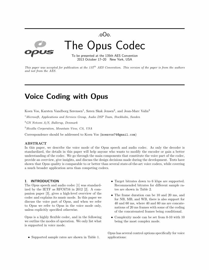
3. ENCODERThe Opus encoder operates on frames of either 10 or20 ms, which are divided into 5 ms subframes. Thefollowing paragraphs describe the main componentsof the encoder. We refer to Figure 1 for an overviewof how the individual functions interact.

3.1. VAD

The Voice Activity Detector (VAD) generates a mea-sure of speech activity by combining the signal-to-noise ratios (SNRs) from 4 separate frequency bands.

1Opus never codes audio above 20 kHz, as that is the upperlimit of human hearing.

AES 135th Convention, New York, USA, 2013 October 17–20

of 10


Fig. 1: Encoder block diagram.

In each band the background noise level is estimatedby smoothing the inverse energy over time frames.Multiplying this smoothed inverse energy with thesubband energy gives the SNR.

3.2. HP Filter

A high-pass (HP) filter with a variable cutofffrequency between 60 and 100 Hz removes low-frequency background and breathing noise. The cut-off frequency depends on the SNR in the lowest fre-quency band of the VAD, and on the smoothed pitchfrequencies found in the pitch analysis, so that highpitched voices will have a higher cutoff frequency.

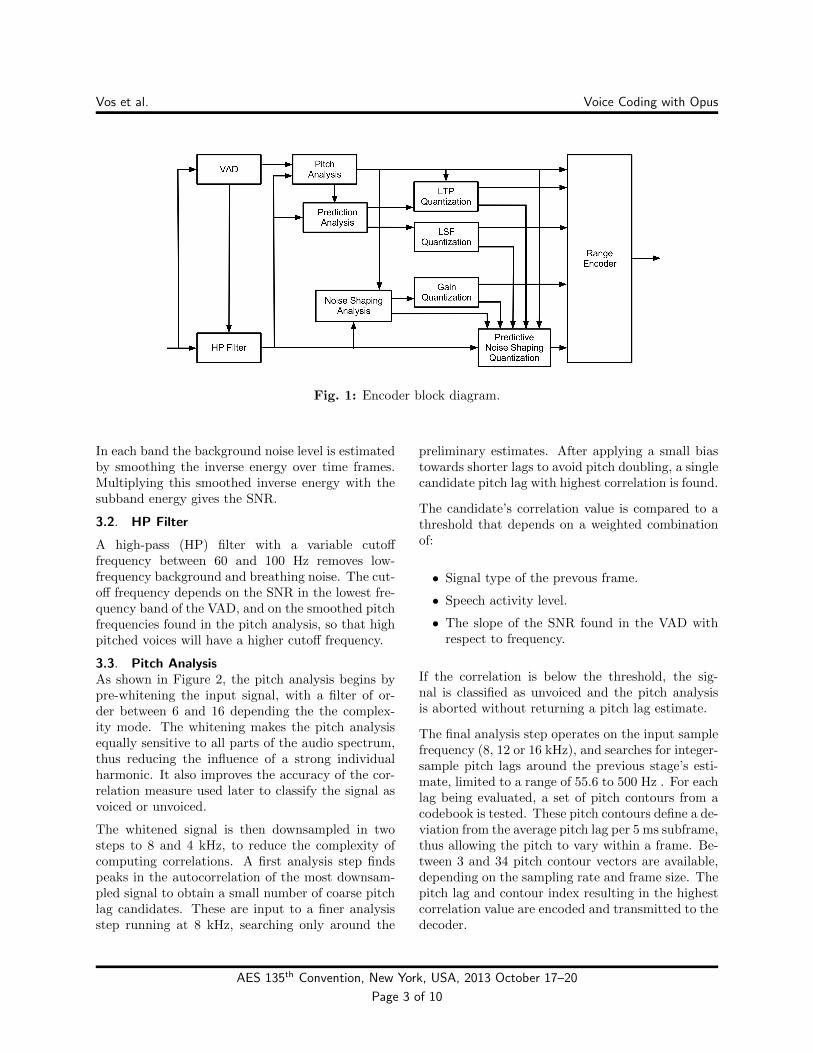
3.3. Pitch AnalysisAs shown in Figure 2, the pitch analysis begins bypre-whitening the input signal, with a filter of or-der between 6 and 16 depending the the complex-ity mode. The whitening makes the pitch analysisequally sensitive to all parts of the audio spectrum,thus reducing the influence of a strong individualharmonic. It also improves the accuracy of the cor-relation measure used later to classify the signal asvoiced or unvoiced.

The whitened signal is then downsampled in twosteps to 8 and 4 kHz, to reduce the complexity ofcomputing correlations. A first analysis step findspeaks in the autocorrelation of the most downsam-pled signal to obtain a small number of coarse pitchlag candidates. These are input to a finer analysisstep running at 8 kHz, searching only around the

preliminary estimates. After applying a small biastowards shorter lags to avoid pitch doubling, a singlecandidate pitch lag with highest correlation is found.

The candidate’s correlation value is compared to athreshold that depends on a weighted combinationof:

• Signal type of the prevous frame.

• Speech activity level.

• The slope of the SNR found in the VAD withrespect to frequency.

If the correlation is below the threshold, the sig-nal is classified as unvoiced and the pitch analysisis aborted without returning a pitch lag estimate.

The final analysis step operates on the input samplefrequency (8, 12 or 16 kHz), and searches for integer-sample pitch lags around the previous stage’s esti-mate, limited to a range of 55.6 to 500 Hz . For eachlag being evaluated, a set of pitch contours from acodebook is tested. These pitch contours define a de-viation from the average pitch lag per 5 ms subframe,thus allowing the pitch to vary within a frame. Be-tween 3 and 34 pitch contour vectors are available,depending on the sampling rate and frame size. Thepitch lag and contour index resulting in the highestcorrelation value are encoded and transmitted to thedecoder.


of 10


Fig. 2: Block diagram of the pitch analysis.

3.3.1. Correlation MeasureMost correlation-based pitch estimators normalizethe correlation with the geometric mean of the en-ergies of the vectors being correlated:

C =xTy√

(xTx · yTy), (1)

whereas Opus normalizes with the arithmetic mean:

COpus =xTy

12 (xTx + yTy)

. (2)

This correlation measures similarity not just inshape, but also in scale. Two vectors with very dif-ferent energies will have a lower correlation, similarto frequency-domain pitch estimators.

3.4. Prediction AnalysisAs described in Section 3.3, the input signal is pre-whitened as part of the pitch analysis. The pre-whitened signal is passed to the prediction analy-sis in addition to the input signal. The signal atthis point is classified as being either voiced or un-voiced. We describe these two cases in Section 3.4.1and 3.4.2.

3.4.1. Voiced SpeechThe long-term prediction (LTP) of voiced signals isimplemented with a fifth order filter. The LTP co-efficients are estimated from the pre-whitened inputsignal with the covariance method for every 5 mssubframe. The coefficients are quantized and used

to filter the input signal (without pre-whitening) tofind an LTP residual. This signal is input to the LPCanalysis, where Burg’s method [5], is used to findshort-term prediction coefficients. Burg’s methodprovides higher prediction gain than the autocorre-lation method and, unlike the covariance method, itproduces stable filter coefficients. The LPC order isNLPC = 16 for FB, SWB, and WB, and NLPC = 10for MB and NB. A novel implementation of Burg’smethod reduces its complexity to near that of theautocorrelation method [6]. Also, the signal in eachsub-frame is scaled by the inverse of the quantizationstep size in that sub-frame before applying Burg’smethod. This is done to find the coefficients thatminimize the number of bits necessary to encode theresidual signal of the frame rather than minimizingthe energy of the residual signal.

Computing LPC coefficients based on the LTP resid-ual rather than on the input signal approximates ajoint optimization of these two sets of coefficients[7]. This increases the prediction gain, thus reducingthe bitrate. Moreover, because the LTP prediction istypically most effective at low frequencies, it reducesthe dynamic range of the AR spectrum defined bythe LPC coefficients. This helps with the numeri-cal properties of the LPC analysis and filtering, andavoids the need for any pre-emphasis filtering foundin other codecs.

3.4.2. Unvoiced SpeechFor unvoiced signals, the pre-whitened signal is dis-


of 10


carded and Burg’s method is used directly on theinput signal.

The LPC coefficients (for either voiced or unvoicedspeech) are converted to Line Spectral Frequencies(LSFs), quantized and used to re-calculate the LPCresidual taking into account the LSF quantizationeffects. Section 3.7 describes the LSF quantization.

3.5. Noise ShapingQuantization noise shaping is used to exploit theproperties of the human auditory system.

A typical state-of-the-art speech encoder determinesthe excitation signal by minimizing the perceptually-weighted reconstruction error. The decoder thenuses a postfilter on the reconstructed signal to sup-press spectral regions where the quantization noiseis expected to be high relative to the signal. Opuscombines these two functions in the encoder’s quan-tizer by applying different weighting filters to theinput and reconstructed signals in the noise shap-ing configuration of Figure 3. Integrating the twooperations on the encoder side not only simplifiesthe decoder, it also lets the encoder use arbitrarilysimple or sophisticated perceptual models to simul-taneously and independently shape the quantizationnoise and boost/suppress spectral regions. Such dif-ferent models can be used without spending bitson side information or changing the bitstream for-mat. As an example of this, Opus uses warped noiseshaping filters at higher complexity settings as thefrequency-dependent resolution of these filters bet-ter matches human hearing [8]. Separating the noiseshaping from the linear prediction also lets us se-lect prediction coefficients that minimize the bitratewithout regard for perceptual considerations.

A diagram of the Noise Shaping Quantization (NSQ)is shown in Figure 3. Unlike typical noise shap-ing quantizers where the noise shaping sits directlyaround the quantizer and feeds back to the input,in Opus the noise shaping compares the input andoutput speech signals and feeds to the input of thequantizer. This was first proposed in Figure 3 of[9]. More details of the NSQ module are describedin Section 3.5.2.

3.5.1. Noise Shaping AnalysisThe Noise Shaping Analysis (NSA) function findsgains and filter coefficients used by the NSQ to shapethe signal spectrum with the following purposes:

• Spectral shaping of the quantization noise sim-ilarly to the speech spectrum to make it lessaudible.

• Suppressing the spectral valleys in between for-mant and harmonic peaks to make the signalless noisy and more predictable.

For each subframe, a quantization gain (or step size)is chosen and sent to the decoder. This quantizationgain determines the tradeoff between quantizationnoise and bitrate.

Furthermore, a compensation gain and a spectral tiltare found to match the decoded speech level and tiltto those of the input signal.

The filtering of the input signal is done using thefilter

H(z) = G · (1− ctilt · z−1) · Wana(z)

Wsyn(z), (3)

where G is the compensation gain, and ctilt is thetilt coefficient in a first order tilt adjustment filter.The analysis filter are for voiced speech given by

Wana(z) =

(1−

NLPC∑k=1

aana(k) · z−k

)(4)

·

(1− z−L ·

2∑k=−2

bana(k) · z−k

), (5)

and similarly for the synthesis filter Wsyn(z). NLPC

is the LPC order and L is the pitch lag in samples.For unvoiced speech, the last term (5) is omitted todisable harmonic noise shaping.

The short-term noise shaping coefficients aana(k)and asyn(k) are calculated from the LPC of the inputsignal a(k) by applying different amounts of band-width expansion, i.e.,

aana(k) = a(k) · gkana, and (6)

asyn(k) = a(k) · gksyn. (7)

The bandwidth expansion moves the roots of theLPC polynomial towards the origin, and therebyflattens the spectral envelope described by a(k).

The bandwidth expansion factors are given by

gana = 0.95− 0.01 · C, and (8)

gsyn = 0.95 + 0.01 · C, (9)


of 10


Fig. 3: Predictive Noise Shaping Quantizer.

where C ∈ [0, 1] is a coding quality control param-eter. By applying more bandwidth expansion tothe analysis part than the synthesis part, we de-emphasize the spectral valleys.

The harmonic noise shaping applied to voiced frameshas three filter taps

bana = Fana · [0.25, 0.5, 0.25], and (10)

bsyn = Fsyn · [0.25, 0.5, 0.25], (11)

where the multipliers Fana and Fsyn ∈ [0, 1] are cal-culated from:

• The coding quality control parameter. Thismakes the decoded signal more harmonic, andthus easier to encode, at low bitrates.

• Pitch correlation. Highly periodic input signalare given more harmonic noise shaping to avoidaudible noise between harmoncis.

• The estimated input SNR below 1 kHz. Thisfilters out background noise for a noise inputsignal by applying more harmonic emphasis.

Similar to the short-term shaping, having Fana <Fsyn emphasizes pitch harmonics and suppresses thesignal in between the harmonics.

The tilt coefficient ctilt is calculated as

ctilt = 0.25 + 0.2625 · V, (12)

where V ∈ [0, 1] is a voice activity level which, inthis context, is forced to 0 for unvoiced speech.

Finally, the compensation gain G is calculated asthe ratio of the prediction gains of the short-termprediction filters aana and asyn.

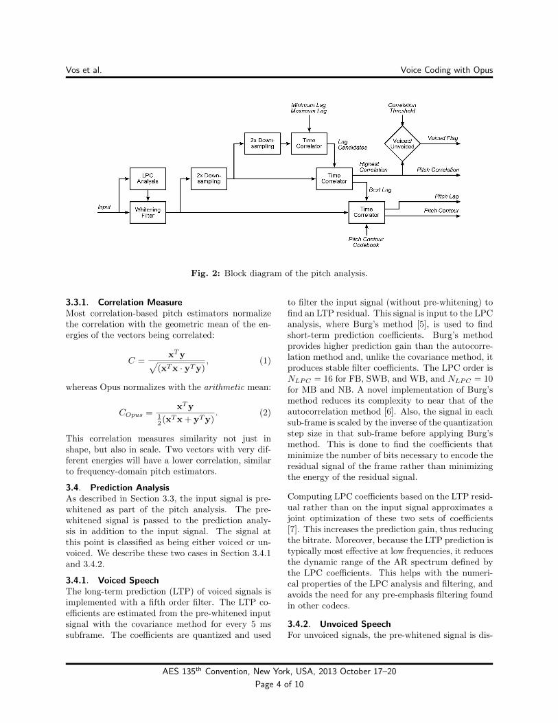
An example of short-term noise shaping of a speechspectrum is shown in Figure 4. The weighted in-put and quantization noise combine to produce anoutput with spectral envelope similar to the inputsignal.

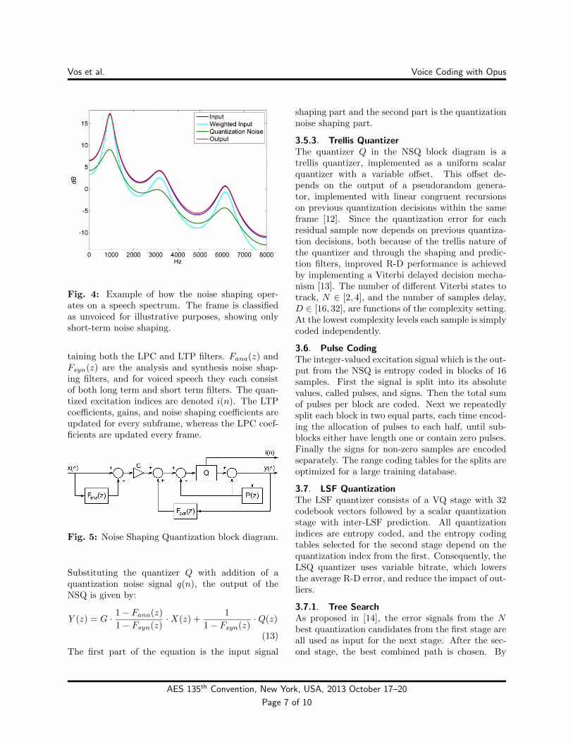
3.5.2. Noise Shaping QuantizationThe NSQ module quantizes the residual signal andthereby generates the excitation signal.

A simplified block diagram of the NSQ is shown inFigure 5. In this figure, P (z) is the predictor con-


of 10


Fig. 4: Example of how the noise shaping oper-ates on a speech spectrum. The frame is classifiedas unvoiced for illustrative purposes, showing onlyshort-term noise shaping.

taining both the LPC and LTP filters. Fana(z) andFsyn(z) are the analysis and synthesis noise shap-ing filters, and for voiced speech they each consistof both long term and short term filters. The quan-tized excitation indices are denoted i(n). The LTPcoefficients, gains, and noise shaping coefficients areupdated for every subframe, whereas the LPC coef-ficients are updated every frame.

Fig. 5: Noise Shaping Quantization block diagram.

Substituting the quantizer Q with addition of aquantization noise signal q(n), the output of theNSQ is given by:

Y (z) = G · 1− Fana(z)

1− Fsyn(z)·X(z) +

1

1− Fsyn(z)·Q(z)

(13)

The first part of the equation is the input signal

shaping part and the second part is the quantizationnoise shaping part.

3.5.3. Trellis QuantizerThe quantizer Q in the NSQ block diagram is atrellis quantizer, implemented as a uniform scalarquantizer with a variable offset. This offset de-pends on the output of a pseudorandom genera-tor, implemented with linear congruent recursionson previous quantization decisions within the sameframe [12]. Since the quantization error for eachresidual sample now depends on previous quantiza-tion decisions, both because of the trellis nature ofthe quantizer and through the shaping and predic-tion filters, improved R-D performance is achievedby implementing a Viterbi delayed decision mecha-nism [13]. The number of different Viterbi states totrack, N ∈ [2, 4], and the number of samples delay,D ∈ [16, 32], are functions of the complexity setting.At the lowest complexity levels each sample is simplycoded independently.

3.6. Pulse CodingThe integer-valued excitation signal which is the out-put from the NSQ is entropy coded in blocks of 16samples. First the signal is split into its absolutevalues, called pulses, and signs. Then the total sumof pulses per block are coded. Next we repeatedlysplit each block in two equal parts, each time encod-ing the allocation of pulses to each half, until sub-blocks either have length one or contain zero pulses.Finally the signs for non-zero samples are encodedseparately. The range coding tables for the splits areoptimized for a large training database.

3.7. LSF QuantizationThe LSF quantizer consists of a VQ stage with 32codebook vectors followed by a scalar quantizationstage with inter-LSF prediction. All quantizationindices are entropy coded, and the entropy codingtables selected for the second stage depend on thequantization index from the first. Consequently, theLSQ quantizer uses variable bitrate, which lowersthe average R-D error, and reduce the impact of out-liers.

3.7.1. Tree SearchAs proposed in [14], the error signals from the Nbest quantization candidates from the first stage areall used as input for the next stage. After the sec-ond stage, the best combined path is chosen. By


of 10


varying the number N , we get a means for adjustingthe trade-off between a low rate-distortion (R-D) er-ror and a high computational complexity. The sameprinciple is used in the NSQ, see Section 3.5.3.

3.7.2. Error SensitivityWhereas input vectors to the first stage are un-weighted, the residual input to the second stage isscaled by the square roots of the Inverse HarmonicMean Weights (IHMWs) proposed by Laroia et al. in[10]. The IHMWs are calculated from the coarsely-quantized reconstruction found in the first stage, sothat encoder and decoder can use the exact sameweights. The application of the weights partiallynormalizes the error sensitivity for the second stageinput vector, and it enables the use of a uniformquantizer with fixed step size to be used withouttoo much loss in quality.

3.7.3. Scalar QuantizationThe second stage uses predictive delayed decisionscalar quantization. The predictor multiplies theprevious quantized residual value by a predictioncoefficient that depends on the vector index fromthe first stage codebook as well as the index for thecurrent scalar in the residual vector. The predictedvalue is subtracted from the second stage input valuebefore quantization and is added back afterwards.This creates a dependency for the current decisionon the previous quantization decision, which againis exploited in a Viterbi-like delayed-decision algo-rithm to choose the sequence of quantization indicesyielding the lowest R-D.

3.7.4. GMM interpretationThe LSF quantizer has similarities with a Gaussianmixture model (GMM) based quantizer [15], wherethe first stage encodes the mean and the secondstage uses the Cholesky decomposition of a tridiag-onal approximation of the correlation matrix. Whatis different is the scaling of the residual vector bythe IHMWs, and the fact that the quantized resid-uals are entropy coded with a entropy table that istrained rather than Gaussian.

3.8. Adaptive Inter-Frame DependencyThe presence of long term prediction, or an AdaptiveCodebook, is known to give challenges when packetlosses occur. The problem with LTP prediction isdue to the impulse response of the filter which canbe much longer than the packet itself.

An often used technique is to reduce the LTP coef-ficients, see e.g. [11], which effectively shortens theimpulse response of the LTP filter.

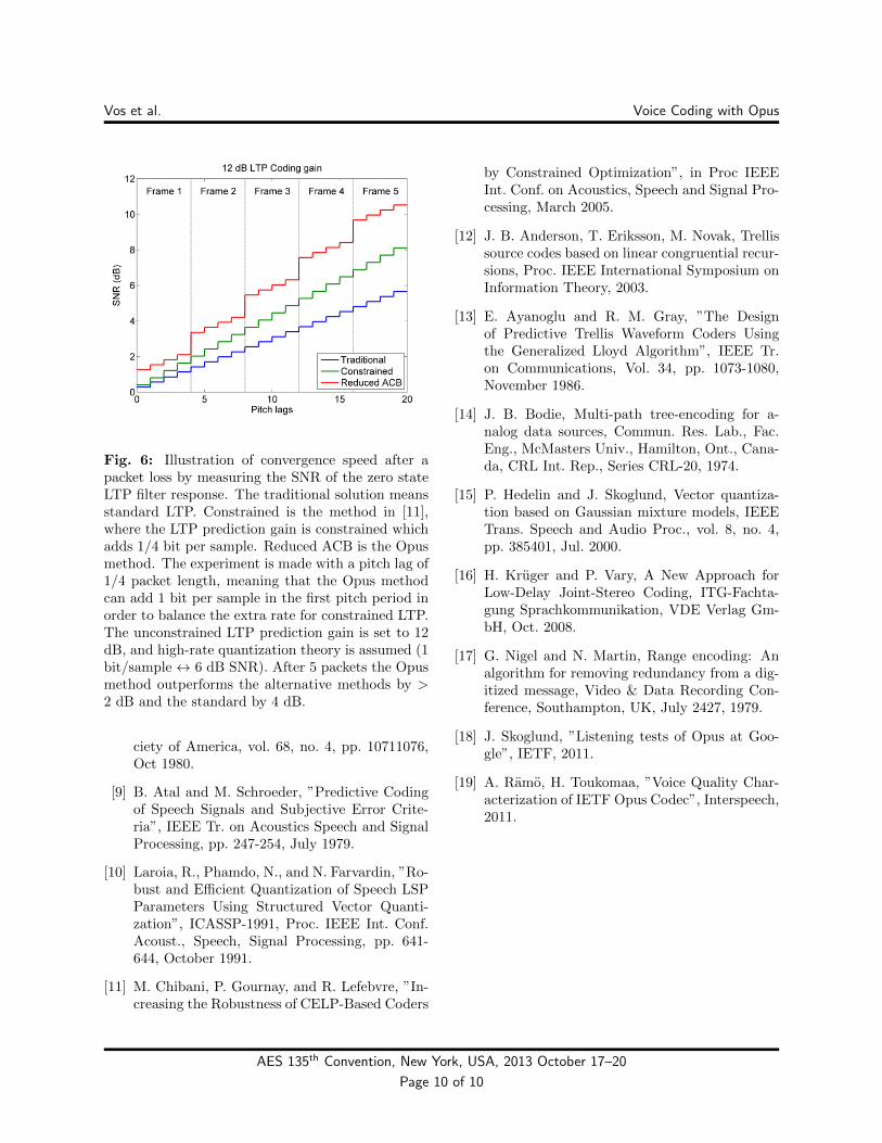
We have solved the problem in a different way; inOpus the LTP filter state is downscaled in the be-ginning of a packet and the LTP coefficients are keptunchanged. Downscaling the LTP state reduces theLTP prediction gain only in the first pitch period inthe packet, and therefore extra bits are only neededfor encoding the higher residual energy during thatfirst pitch period. Because of Jensens inequality, itsbetter to fork out the bits upfront and be done withit. The scaling factor is quantized to one of threevalues and is thus transmitted with very few bits.

Compared to scaling the LTP coefficients, downscal-ing the LTP state gives a more efficient trade-off be-tween increased bit rate caused by lower LTP pre-diction gain and encoder/decoder resynchronizationspeed which is illustrated in Figure 6.

3.9. Entropy CodingThe quantized parameters and the excitation signalare all entropy coded using range coding, see [17].

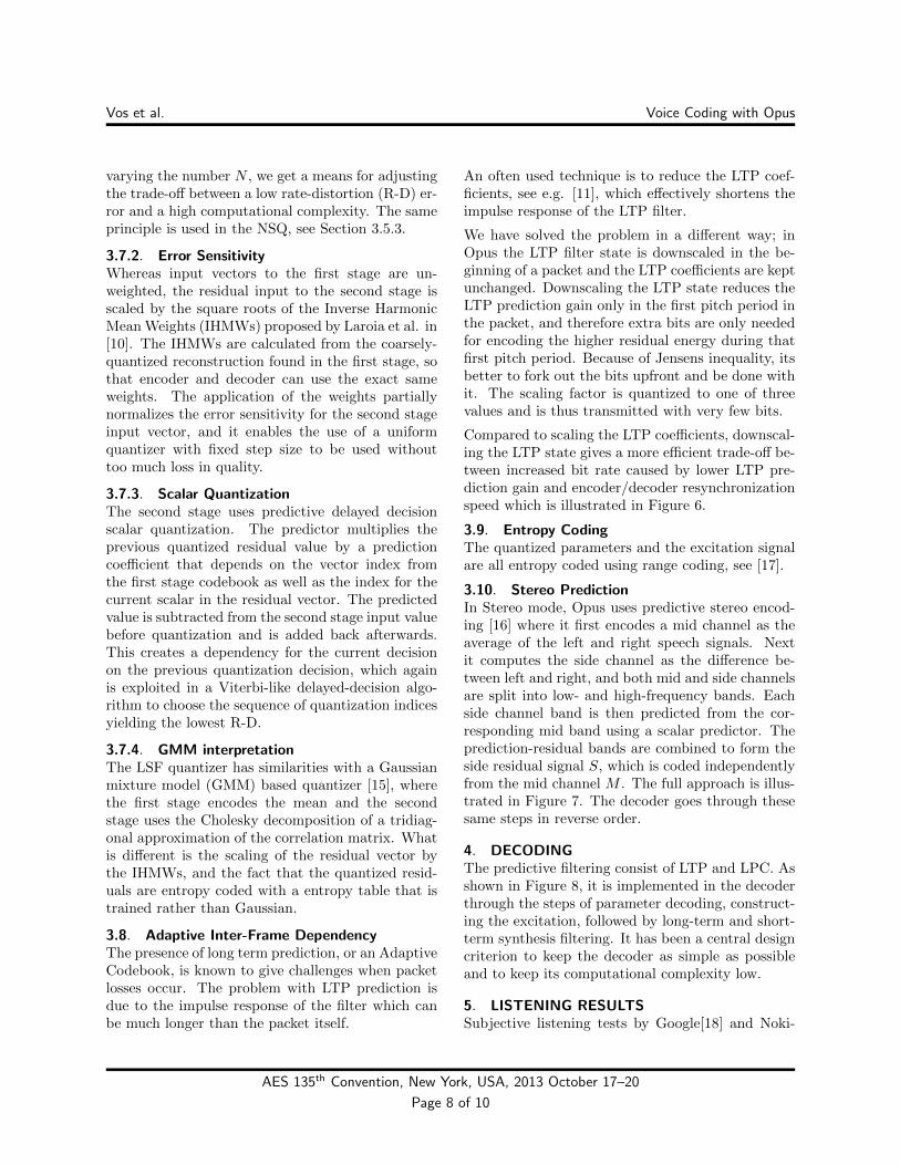
3.10. Stereo PredictionIn Stereo mode, Opus uses predictive stereo encod-ing [16] where it first encodes a mid channel as theaverage of the left and right speech signals. Nextit computes the side channel as the difference be-tween left and right, and both mid and side channelsare split into low- and high-frequency bands. Eachside channel band is then predicted from the cor-responding mid band using a scalar predictor. Theprediction-residual bands are combined to form theside residual signal S, which is coded independentlyfrom the mid channel M . The full approach is illus-trated in Figure 7. The decoder goes through thesesame steps in reverse order.

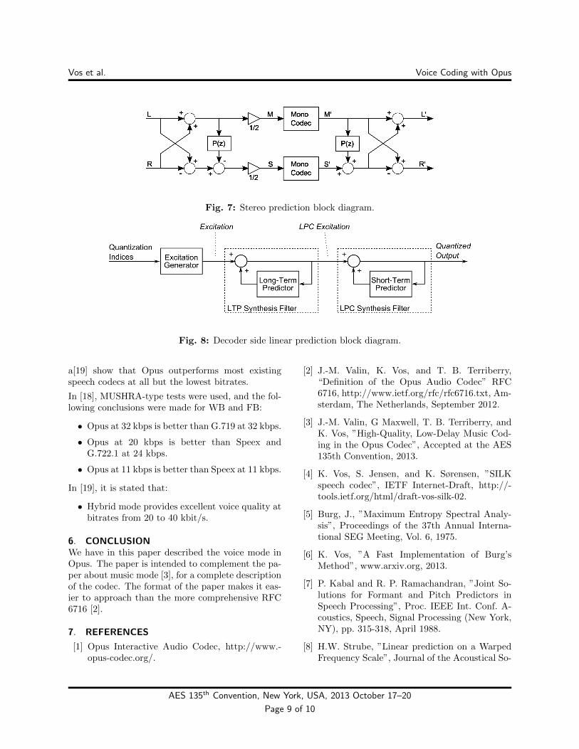
4. DECODINGThe predictive filtering consist of LTP and LPC. Asshown in Figure 8, it is implemented in the decoderthrough the steps of parameter decoding, construct-ing the excitation, followed by long-term and short-term synthesis filtering. It has been a central designcriterion to keep the decoder as simple as possibleand to keep its computational complexity low.

5. LISTENING RESULTSSubjective listening tests by Google[18] and Noki-


of 10


Fig. 7: Stereo prediction block diagram.

Fig. 8: Decoder side linear prediction block diagram.

a[19] show that Opus outperforms most existingspeech codecs at all but the lowest bitrates.

In [18], MUSHRA-type tests were used, and the fol-lowing conclusions were made for WB and FB:

• Opus at 32 kbps is better than G.719 at 32 kbps.

• Opus at 20 kbps is better than Speex andG.722.1 at 24 kbps.

• Opus at 11 kbps is better than Speex at 11 kbps.

In [19], it is stated that:

• Hybrid mode provides excellent voice quality atbitrates from 20 to 40 kbit/s.

6. CONCLUSIONWe have in this paper described the voice mode inOpus. The paper is intended to complement the pa-per about music mode [3], for a complete descriptionof the codec. The format of the paper makes it eas-ier to approach than the more comprehensive RFC6716 [2].

7. REFERENCES

[1] Opus Interactive Audio Codec, http://www.-opus-codec.org/.

[2] J.-M. Valin, K. Vos, and T. B. Terriberry,“Definition of the Opus Audio Codec” RFC6716, http://www.ietf.org/rfc/rfc6716.txt, Am-sterdam, The Netherlands, September 2012.

[3] J.-M. Valin, G Maxwell, T. B. Terriberry, andK. Vos, ”High-Quality, Low-Delay Music Cod-ing in the Opus Codec”, Accepted at the AES135th Convention, 2013.

[4] K. Vos, S. Jensen, and K. Sørensen, ”SILKspeech codec”, IETF Internet-Draft, http://-tools.ietf.org/html/draft-vos-silk-02.

[5] Burg, J., ”Maximum Entropy Spectral Analy-sis”, Proceedings of the 37th Annual Interna-tional SEG Meeting, Vol. 6, 1975.

[6] K. Vos, ”A Fast Implementation of Burg’sMethod”, www.arxiv.org, 2013.

[7] P. Kabal and R. P. Ramachandran, ”Joint So-lutions for Formant and Pitch Predictors inSpeech Processing”, Proc. IEEE Int. Conf. A-coustics, Speech, Signal Processing (New York,NY), pp. 315-318, April 1988.

[8] H.W. Strube, ”Linear prediction on a WarpedFrequency Scale”, Journal of the Acoustical So-


of 10


Fig. 6: Illustration of convergence speed after apacket loss by measuring the SNR of the zero stateLTP filter response. The traditional solution meansstandard LTP. Constrained is the method in [11],where the LTP prediction gain is constrained whichadds 1/4 bit per sample. Reduced ACB is the Opusmethod. The experiment is made with a pitch lag of1/4 packet length, meaning that the Opus methodcan add 1 bit per sample in the first pitch period inorder to balance the extra rate for constrained LTP.The unconstrained LTP prediction gain is set to 12dB, and high-rate quantization theory is assumed (1bit/sample ↔ 6 dB SNR). After 5 packets the Opusmethod outperforms the alternative methods by >2 dB and the standard by 4 dB.

ciety of America, vol. 68, no. 4, pp. 10711076,Oct 1980.

[9] B. Atal and M. Schroeder, ”Predictive Codingof Speech Signals and Subjective Error Crite-ria”, IEEE Tr. on Acoustics Speech and SignalProcessing, pp. 247-254, July 1979.

[10] Laroia, R., Phamdo, N., and N. Farvardin, ”Ro-bust and Efficient Quantization of Speech LSPParameters Using Structured Vector Quanti-zation”, ICASSP-1991, Proc. IEEE Int. Conf.Acoust., Speech, Signal Processing, pp. 641-644, October 1991.

[11] M. Chibani, P. Gournay, and R. Lefebvre, ”In-creasing the Robustness of CELP-Based Coders

by Constrained Optimization”, in Proc IEEEInt. Conf. on Acoustics, Speech and Signal Pro-cessing, March 2005.

[12] J. B. Anderson, T. Eriksson, M. Novak, Trellissource codes based on linear congruential recur-sions, Proc. IEEE International Symposium onInformation Theory, 2003.

[13] E. Ayanoglu and R. M. Gray, ”The Designof Predictive Trellis Waveform Coders Usingthe Generalized Lloyd Algorithm”, IEEE Tr.on Communications, Vol. 34, pp. 1073-1080,November 1986.

[14] J. B. Bodie, Multi-path tree-encoding for a-nalog data sources, Commun. Res. Lab., Fac.Eng., McMasters Univ., Hamilton, Ont., Cana-da, CRL Int. Rep., Series CRL-20, 1974.

[15] P. Hedelin and J. Skoglund, Vector quantiza-tion based on Gaussian mixture models, IEEETrans. Speech and Audio Proc., vol. 8, no. 4,pp. 385401, Jul. 2000.

[16] H. Kruger and P. Vary, A New Approach forLow-Delay Joint-Stereo Coding, ITG-Fachta-gung Sprachkommunikation, VDE Verlag Gm-bH, Oct. 2008.

[17] G. Nigel and N. Martin, Range encoding: Analgorithm for removing redundancy from a dig-itized message, Video & Data Recording Con-ference, Southampton, UK, July 2427, 1979.

[18] J. Skoglund, ”Listening tests of Opus at Goo-gle”, IETF, 2011.

[19] A. Ramo, H. Toukomaa, ”Voice Quality Char-acterization of IETF Opus Codec”, Interspeech,2011.


of 10

ooo. the opus codec · 3.3. pitch analysis as shown in figure 2, the pitch analysis begins by...

Documents