Online Monitoring of Supercapacitor Ageing

Authors:

Zhihao SHI, François AUGER, Emmanuel SCHAEFFER, Philippe GUILLEMET, Luc LORON

1

Réunion inter GDR inter GT – 21/11/2013

2

Content

� Introduction

� Applications of EDLCs (Electric Double Layer Capacitors)

� Advantages of EDLCs

� EDLCs models

� EDLCs Ageing

� Online Identification

� Principle

� Mathematical model of EDLCs system

� Observability of EDLCs system

� Identification methods

� Experimental Results

� Conclusion and future work

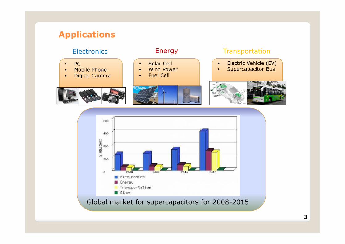
• PC• Mobile Phone• Digital Camera

Electronics Energy

• Solar Cell• Wind Power• Fuel Cell

Transportation

• Electric Vehicle (EV)• Supercapacitor Bus

Global market for supercapacitors for 2008-2015

Applications

33

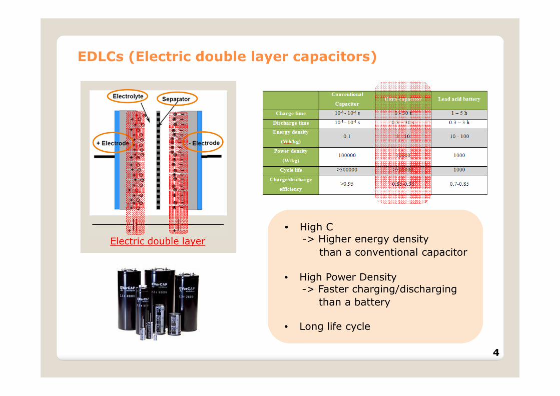
EDLCs (Electric double layer capacitors)

Electric double layer

• High C -> Higher energy density

• High Power Density -> Faster charging/discharging

• Long life cycle

than a conventional capacitor

than a battery

4

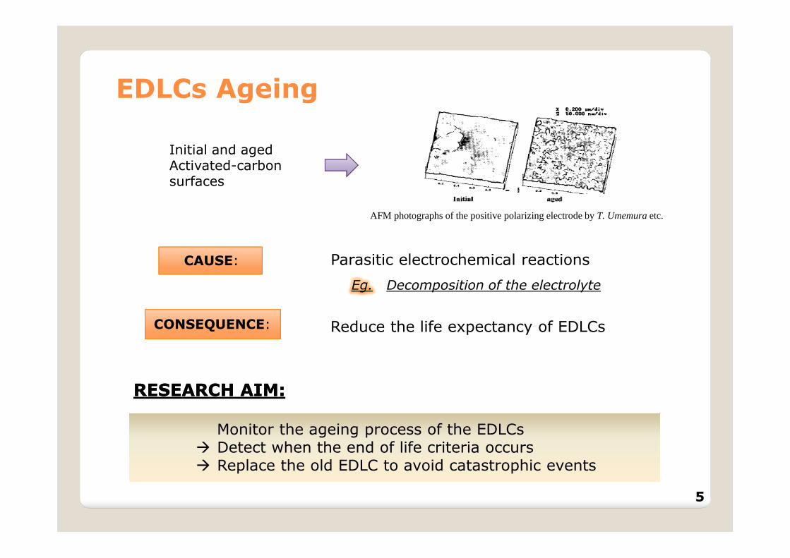
EDLCs Ageing

CAUSE:

CONSEQUENCE:

Parasitic electrochemical reactions

Eg. Decomposition of the electrolyte

Reduce the life expectancy of EDLCs

RESEARCH AIM:RESEARCH AIM:

Monitor the ageing process of the EDLCs � Detect when the end of life criteria occurs � Replace the old EDLC to avoid catastrophic events

Initial and aged Activated-carbon surfaces

AFM photographs of the positive polarizing electrode by T. Umemuraetc.

5

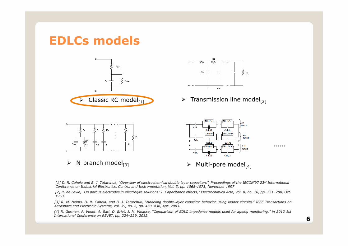
EDLCs models

� Classic RC model[1] � Transmission line model[2]

[1] D. R. Cahela and B. J. Tatarchuk, “Overview of electrochemical double layer capacitors”, Proceedings of the IECON’97 23rd International Conference on Industrial Electronics, Control and Instrumentation, Vol. 3, pp. 1068-1073, November 1997

[2] R. de Levie, “On porous electrodes in electrolyte solutions: I. Capacitance effects,” Electrochimica Acta, vol. 8, no. 10, pp. 751–780, Oct. 1963.

� N-branch model[3] � Multi-pore model[4]

……

[3] R. M. Nelms, D. R. Cahela, and B. J. Tatarchuk, “Modeling double-layer capacitor behavior using ladder circuits,” IEEE Transactions onAerospace and Electronic Systems, vol. 39, no. 2, pp. 430–438, Apr. 2003.

[4] R. German, P. Venet, A. Sari, O. Briat, J. M. Vinassa, “Comparison of EDLC impedance models used for ageing monitoring,” in 2012 1stInternational Conference on REVET, pp. 224–229, 2012.

6

An example:

RS

C

End of life

End of life

Ageing Variation of Parameters

Visible by

State of Health(SOH)

State of Health(SOH)

State of Charge(SOC)

State of Charge(SOC)

E �1

2CV

�

Estimate

Quantification of EDLCs Ageing

7

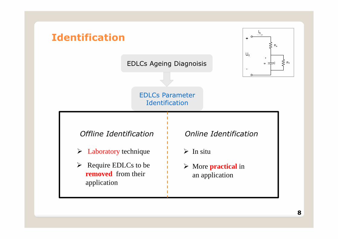
Identification

EDLCs Ageing DiagnoisisEDLCs Ageing Diagnoisis

EDLCs Parameter Identification

EDLCs Parameter Identification

Offline Identification Online Identification

� Laboratorytechnique

� Require EDLCs to be removed from their application

� More practical in an application

� In situ

8

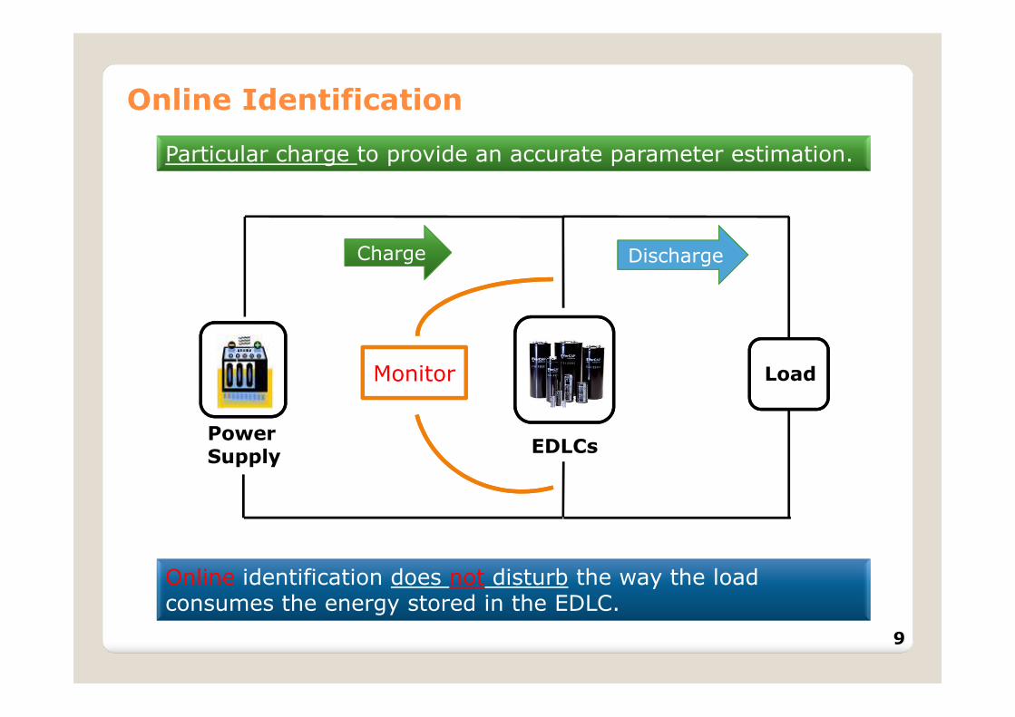
Online Identification

Charge

Power Supply

EDLCs

Monitor

Particular charge to provide an accurate parameter estimation.

Load

Discharge

Online identification does not disturb the way the loadconsumes the energy stored in the EDLC.

9

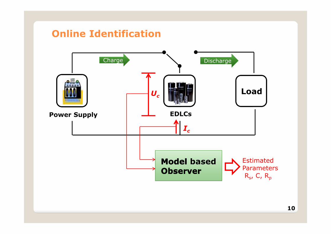
Online Identification

Load

ChargeCharge DischargeDischarge

Power Supply EDLCs

Uc

Ic

Model basedObserver

EstimatedParameters Rs, C, Rp

ModelModelObserverObserver

10

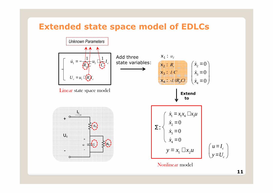
Extended state space model of EDLCs

1 1

1 1c

p

u u IR C C

= − +&

1c s cU u R I= +

x2 : Rs

x3 : 1/C

x4 : -1/(RpC)

Add three state variables:

2

3

4

0

0

0

x

x

x

= = =

&

&

&

1 1 4 3

2

3

4

0

0

0

x x x x u

x

x

x

= +===

&

&

&

&

1 2y x x u= +

Σ:

Linear state space model

Nonlinear model

c

c

u I

y U

= =

x1 : u1

Unknown Parameters

Extend to

11

Online state and parameter estimation

x1 = u1

x2 = Rs

x3 = 1/C

x4 = -1/(RpC)

1 1 4 3

2

3

4

0

0

0

x x x x u

x

x

x

= +===

&

&

&

&

1 2y x x u= +

Σ:

Extended state space model

Estimatedparameters

Model basedObserver

Rs; 1/C; -1/(RpC)

c

c

u I

y U

= =

?

Estimatedinternal state State of charge

estimation

12

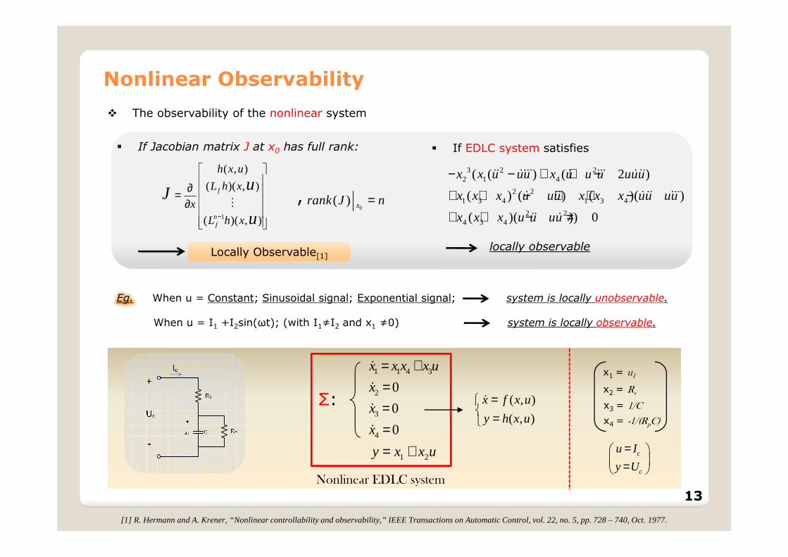
Nonlinear Observability

� The observability of the nonlinear system

1 1 4 3

2

3

4

0

0

0

x x x x u

x

x

x

= +===

&

&

&

&

1 2y x x u= +

Σ:

Nonlinear EDLC system

x4 = -1/(RpC)

x1 = u1

x2 = Rs

x3 = 1/C

c

c

u I

y U

= =

3 2 22 1 4

2 21 3 4 1 3 4

2 24 3 4

( ( ) ( 2 )

( ) ( ) ( )( )

( )( )) 0

x x u uu x u u u uuu

x x x u uu x x x uu uu

x x x u u uu

− − + + −

+ + − + + −

+ + − ≠

&& &&&& & &&& &&&

& && &&& &&&

&& &

� If EDLC system satisfies

locally observable

� If Jacobian matrix J at x0 has full rank:

1

( , )

( )( , )

( )( , )

f

nf

h x u

L h x

x

L h x

uJ

u−

∂ = ∂

M 0( ) xrank J n=

Locally Observable[1]Locally Observable[1]

,

[1] R. Hermann and A. Krener, “Nonlinear controllability and observability,” IEEE Transactions on Automatic Control, vol. 22, no. 5, pp. 728 – 740, Oct. 1977.

Eg. When u = Constant; Sinusoidal signal; Exponential signal; system is locally unobservable.

When u = I1 +I2sin(ωt); (with I1≠I2 and x1 ≠0) system is locally observable.

( , )

( , )

x f x u

y h x u

= =

&

13

14

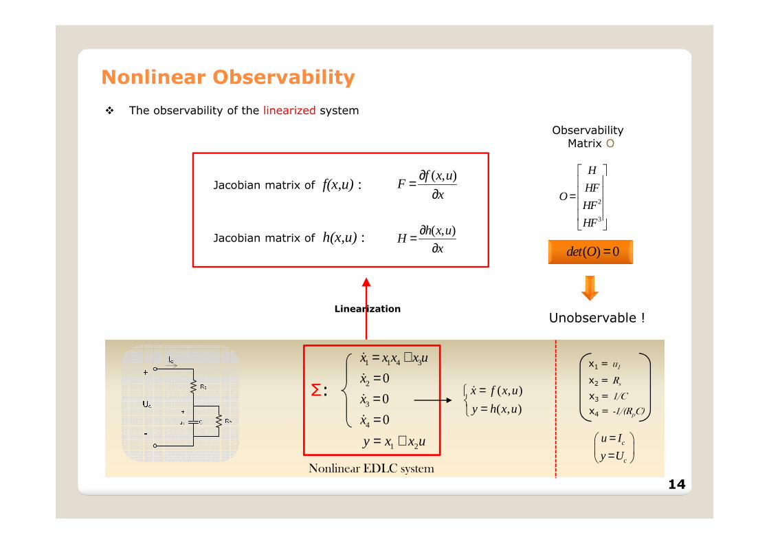
Nonlinear Observability

� The observability of the linearized system

( , )f x uF

x

∂=∂

( , )h x uH

x

∂=∂

ObservabilityMatrix O

2

3

H

HFO

HF

HF

=

( ) 0det O =

LinearizationUnobservable !

Jacobian matrix of f(x,u) :

Jacobian matrix of h(x,u) :

1 1 4 3

2

3

4

0

0

0

x x x x u

x

x

x

= +===

&

&

&

&

1 2y x x u= +

Σ:

Nonlinear EDLC system

x4 = -1/(RpC)

x1 = u1

x2 = Rs

x3 = 1/C

c

c

u I

y U

= =

( , )

( , )

x f x u

y h x u

= =

&

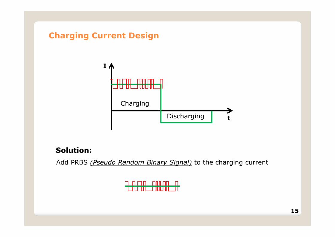
Charging Current Design

Charging

Discharging t

I

Solution:

Add PRBS (Pseudo Random Binary Signal) to the charging current

15

Extended Kalman Observer (EKO)

( , )

( , )

x f x u w

y h x u v

= += +

&Extended system dynamics :

Measured output :

w : Process noise

v : Sensor noise

x̂ : states estimated by the observer

1TK PH R−= 1T TP FP PF PH R HP Q−= + − +&

EDLCs

K

EKO

ˆ ˆ ˆ( , ) ( )x f x u K y y= + −&

ˆ ˆ( , )y h x u=

nv

ni

ˆy y−+

-1

2

3

4

ˆ

ˆ

ˆ

ˆ

x

x

x

x

Calculation of K:

IIIIcccc UUUUcccc

for

x1 = u1

x2 = Rs

x3 = 1/C

x4 = -1/(RpC)

Parameter Estimation

, with

16

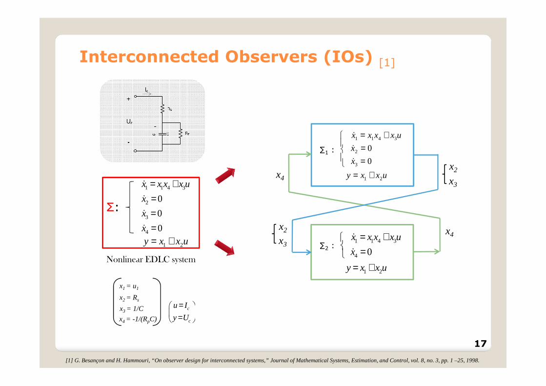
Interconnected Observers (IOs) [1]

Nonlinear EDLC system

1 1 4 3

2

3

4

0

0

0

x x x x u

x

x

x

= +===

&

&

&

&

1 2y x x u= +

Σ:

∑1 :

1 1 4 3

2

3

1 2

0

0

x x x x u

x

x

y x x u

= + = =

= +

&

&

&

1 1 4 3

4

1 2

0

x x x x u

x

y x x u

= + =

= +

&

&∑2 :

x4

x4 = -1/(RpC)

x1 = u1

x2 = Rs

x3 = 1/C c

c

u I

y U

= =

x2

x3

x2

x3x4

[1] G. Besançon and H. Hammouri, “On observer design for interconnected systems,” Journal of Mathematical Systems, Estimation, and Control, vol. 8, no. 3, pp. 1 –25, 1998.

17

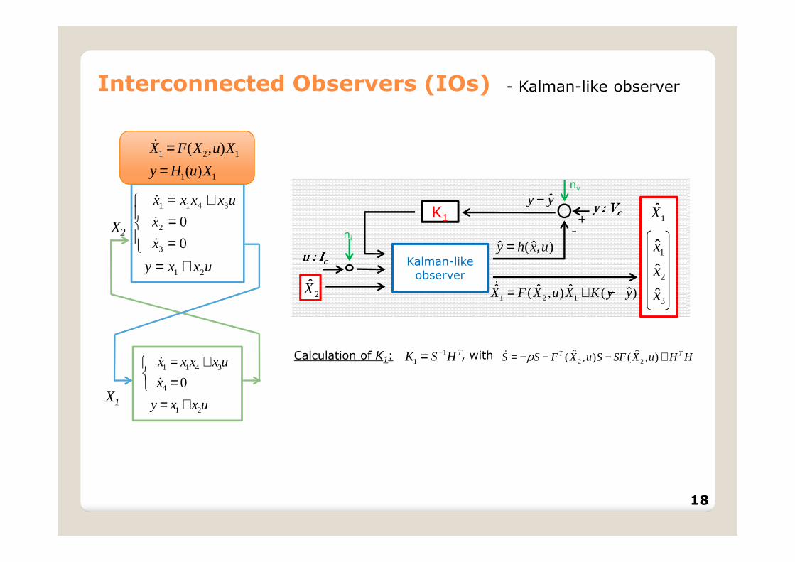
Interconnected Observers (IOs)

1 1 4 3

2

3

1 2

0

0

x x x x u

x

x

y x x u

= + = =

= +

&

&

&

X2

K1

Kalman-like observer

1 2 1ˆ ˆ ˆ ˆ( , ) ( )X F X u X K y y= + −&

ˆ ˆ( , )y h x u=

nv

ni

ˆy y−+

-

1

2

3

ˆ

ˆ

ˆ

x

x

x

uuuu : : : : IIIIcccc

y : y : y : y : VVVVcccc

1 2 1

1 1

( , )

( )

X F X u X

y H u X

==

&

1 1 4 3

4

1 2

0

x x x x u

x

y x x u

= + =

= +

&

&

X1

1X̂

11

TK S H−= 2 2ˆ ˆ( , ) ( , )T TS S F X u S SF X u H Hρ= − − − +&Calculation of K1:

2X̂

, with

- Kalman-like observer

18

1 1 4 3

4

1 2

0

x x x x u

x

y x x u

= + =

= +

&

&

1 1 4 3

2

3

1 2

0

0

x x x x u

x

x

y x x u

= + = =

= +

&

&

&

X2

X1

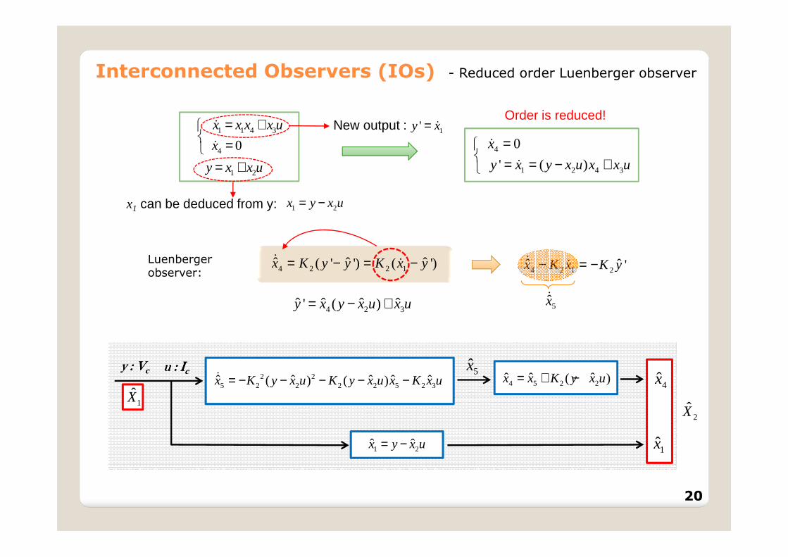
Interconnected Observers (IOs) - Reduced order Luenberger observer

19

2X̂

Interconnected Observers (IOs)

1 1 4 3

4

1 2

0

x x x x u

x

y x x u

= + =

= +

&

&

1 2x y x u= −

1'y x= &New output :

4

1 2 4 3

0

' ( )

x

y x y x u x x u

= = = − +

&

&

Order is reduced!

x1 can be deduced from y:

- Reduced order Luenberger observer

4 2 2 1ˆ ˆ ˆ( ' ') ( ')x K y y K x y= − = −& &

4 2 3ˆ ˆ ˆ ˆ' ( )y x y x u x u= − +

4 2 1 2ˆ ˆ 'x K x K y− = −& &

5x̂&

2 25 2 2 2 2 5 2 3ˆ ˆ ˆ ˆ ˆ( ) ( )x K y x u K y x u x K x u= − − − − −&

4x̂uuuu : : : : IIIIccccy : y : y : y : VVVVcccc 5x̂

4 5 2 2ˆ ˆ ˆ( )x x K y x u= + −

1 2ˆ ˆx y x u= − 1x̂

Luenbergerobserver:

1X̂

20

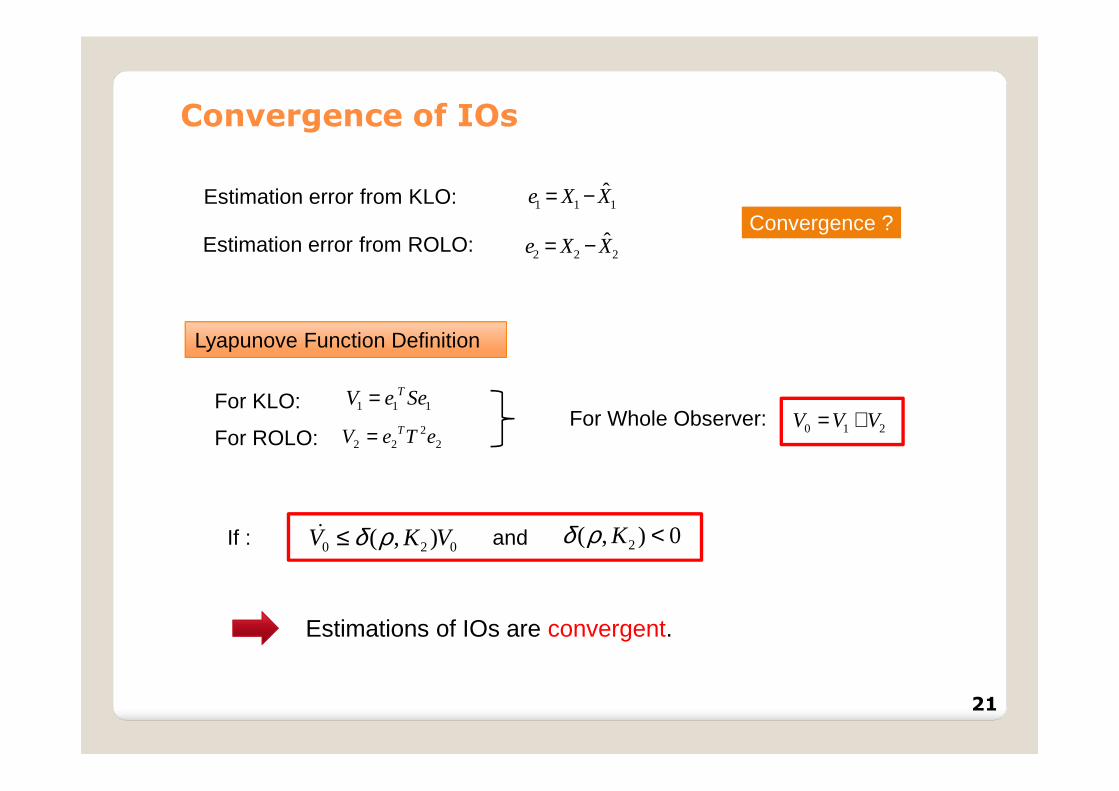
Convergence of IOs

1 1 1TV e Se=

1 1 1ˆe X X= −Estimation error from KLO:

Estimation error from ROLO: 2 2 2ˆe X X= −

Convergence ?

Lyapunove Function Definition

For ROLO: 22 2 2

TV e T e=For Whole Observer: 0 1 2V V V= +

0 2 0( , )V K Vδ ρ≤&

For KLO:

If : 2( , ) 0Kδ ρ <and

Estimations of IOs are convergent.

21

Comparison of the two kinds of observers

Extended Kalman Observer (EKO) Interconnected Observers (IOs)

� Is able to estimate the parameters online

� Is able to estimate the parameters online

� The convergence is guaranteed

� It is difficult to prove its convergence.

� More tuning parameters � Less tuning parameters

22

Ageing Experiments

� EDLC tested:

� Ageing test bench:

Stoves VSPVoltage source

Nichicon UM series 2,7V/1F

Thermostat

Ageing Acceleration

60˚C

12 weeks ageing

23

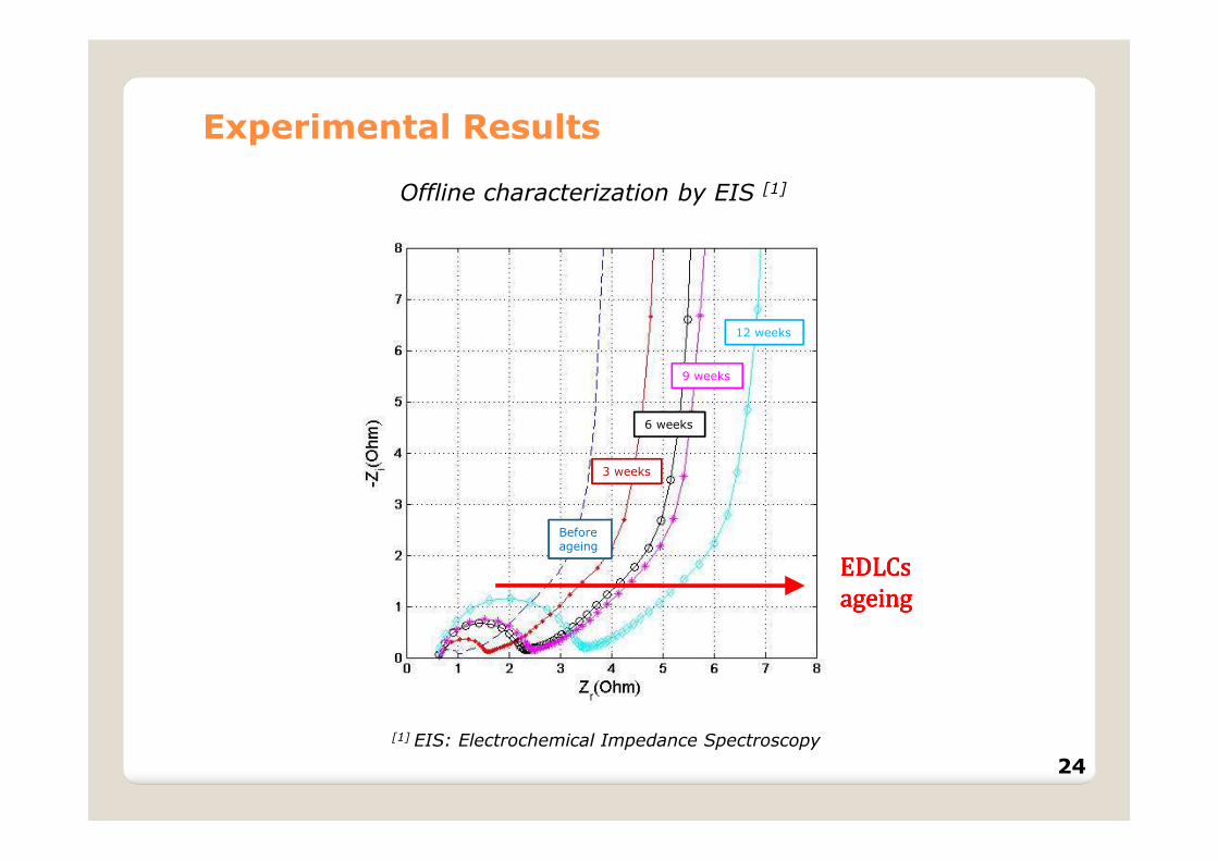
Experimental Results

Offline characterization by EIS [1]

Before ageing

6 weeks

3 weeks

9 weeks

12 weeks

[1] EIS: Electrochemical Impedance Spectroscopy

EDLCs EDLCs EDLCs EDLCs

ageingageingageingageing

24

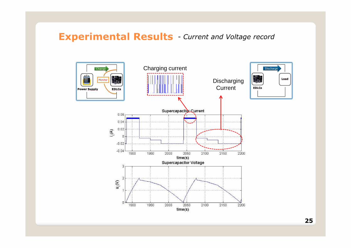
Charging current

DischargingCurrent

- Current and Voltage record

25

Experimental Results

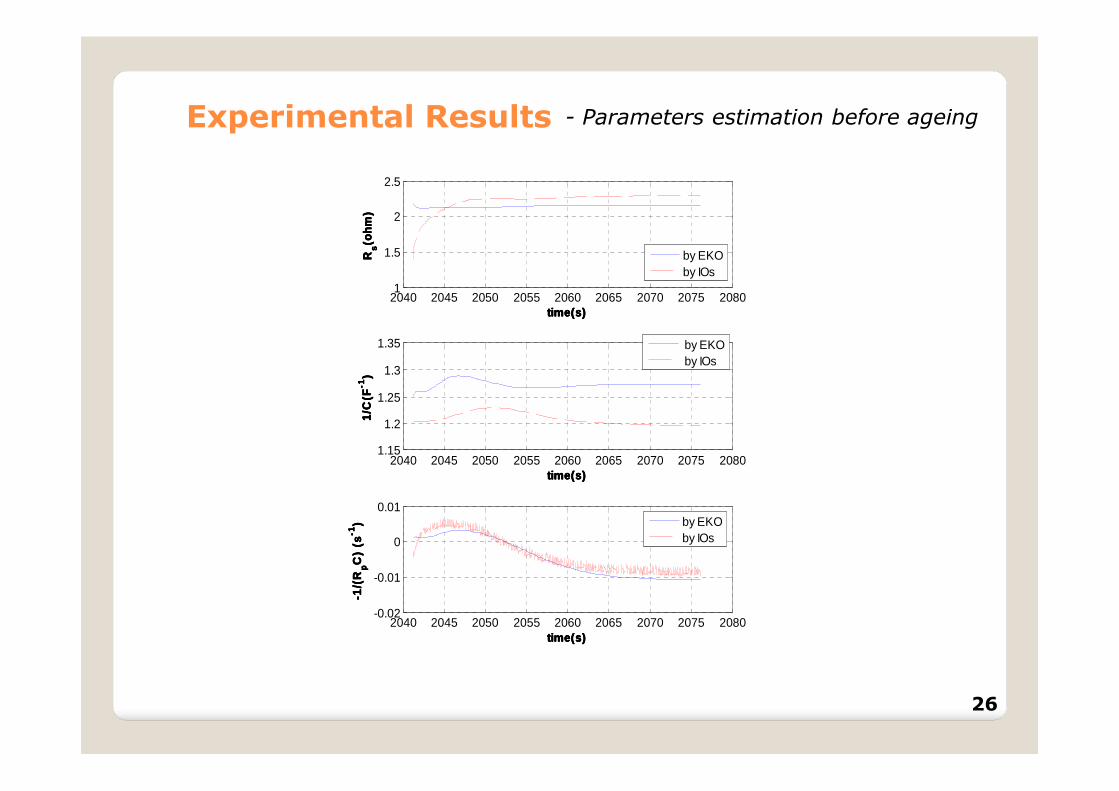
- Parameters estimation before ageing

2040 2045 2050 2055 2060 2065 2070 2075 20801

1.5

2

2.5

time(s)time(s)time(s)time(s)

RR RRss ss(o

hm

)(o

hm

)(o

hm

)(o

hm

)

by EKOby IOs

2040 2045 2050 2055 2060 2065 2070 2075 20801.15

1.2

1.25

1.3

1.35

time(s)time(s)time(s)time(s)

1/C

(F1

/C(F

1/C

(F1

/C(F

-- -- 11 11)) ))

by EKO by IOs

2040 2045 2050 2055 2060 2065 2070 2075 2080-0.02

-0.01

0

0.01

time(s)time(s)time(s)time(s)

-1/(

R-1

/(R

-1/(

R-1

/(R

pp ppC

) (s

C)

(sC

) (s

C)

(s-- -- 11 11

)) ))

by EKOby IOs

26

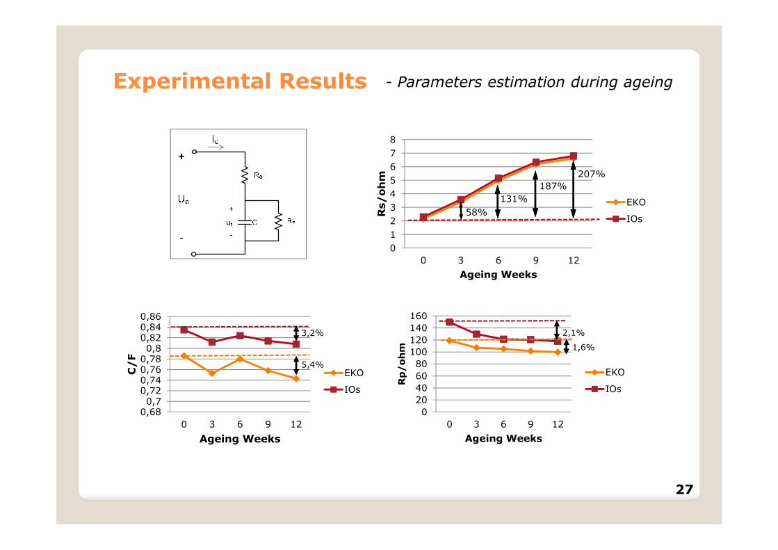
Experimental Results

0

1

2

3

4

5

6

7

8

0 3 6 9 12

Rs/

oh

m

Ageing Weeks

EKO

IOs58%

131%

187%

207%

0,680,7

0,720,740,760,780,8

0,820,840,86

0 3 6 9 12

C/

F

Ageing Weeks

EKO

IOs

0

20

40

60

80

100

120

140

160

0 3 6 9 12

Rp

/o

hm

Ageing Weeks

EKO

IOs

3,2%

5,4%

2,1%

1,6%

- Parameters estimation during ageing

27

Experimental Results

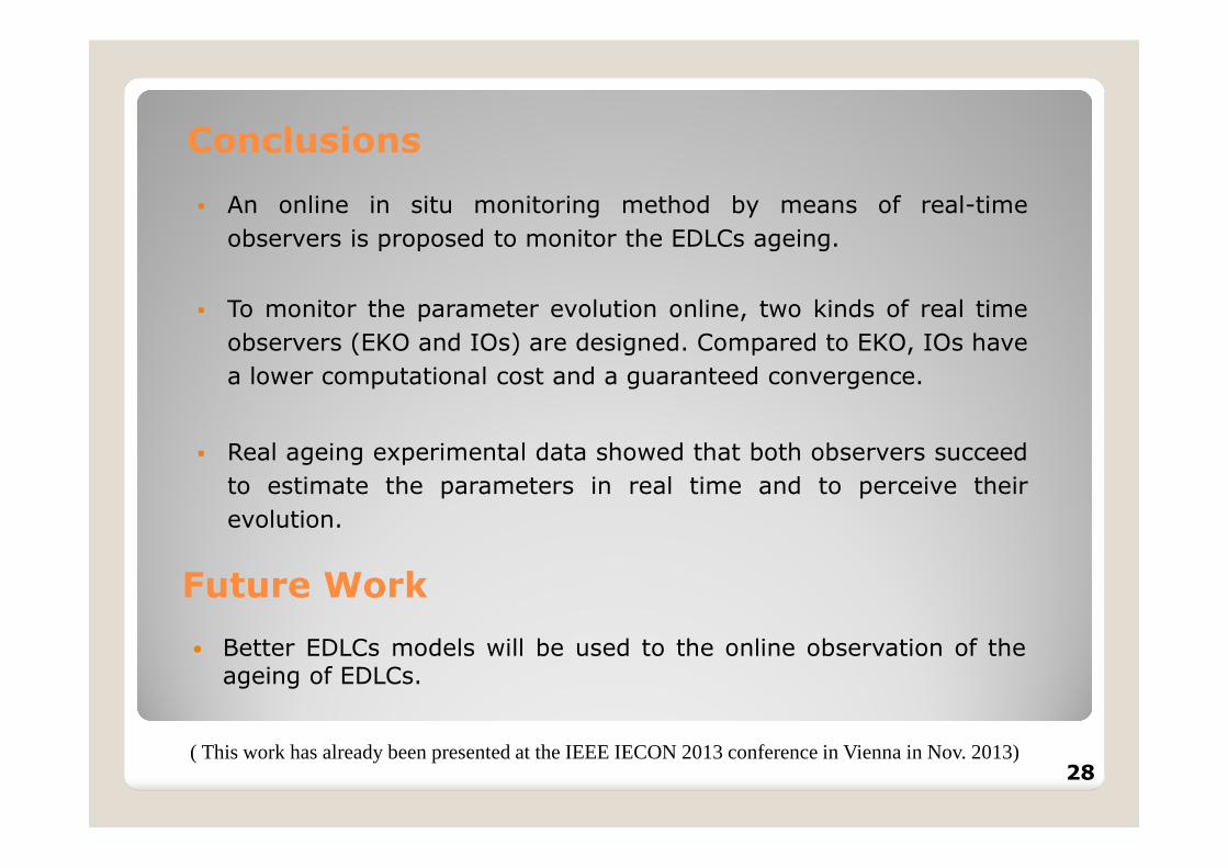
Conclusions

� An online in situ monitoring method by means of real-time

observers is proposed to monitor the EDLCs ageing.

� To monitor the parameter evolution online, two kinds of real time

observers (EKO and IOs) are designed. Compared to EKO, IOs have

a lower computational cost and a guaranteed convergence.

� Real ageing experimental data showed that both observers succeed

to estimate the parameters in real time and to perceive their

evolution.

Future Work

� Better EDLCs models will be used to the online observation of theageing of EDLCs.

28( This work has already been presented at the IEEE IECON 2013 conference in Vienna in Nov. 2013)

E-mail: zhihao.shi@univ-nantes.fr

Thank you for your Thank you for your Thank you for your Thank you for your attention!attention!attention!attention!