online entity resolution using an oracle - vldb · online entity resolution using an oracle ......
TRANSCRIPT
Online Entity Resolution Using an Oracle
Donatella Firmani∗Univ. of Rome “Tor Vergata”
Barna Saha†UMass Amherst
Divesh SrivastavaAT&T Labs – Research
ABSTRACTEntity resolution (ER) is the task of identifying all records in adatabase that refer to the same underlying entity. This is an expen-sive task, and can take a significant amount of money and time; theend-user may want to take decisions during the process, rather thanwaiting for the task to be completed. We formalize an online ver-sion of the entity resolution task, and use an oracle which correctlylabels matching and non-matching pairs through queries. In thissetting, we design algorithms that seek to maximize progressive re-call, and develop a novel analysis framework for prior proposalson entity resolution with an oracle, beyond their worst case guaran-tees. Finally, we provide both theoretical and experimental analysisof the proposed algorithms.
1. INTRODUCTIONEntity resolution (ER, record linkage, deduplication, etc.) seeks
to identify which records in a data set refer to the same underly-ing real-world entity [6, 8]. It is a challenging problem for manyreasons, intricate because of our ability to represent and misrep-resent information about real-world entities in very diverse ways.For example, collecting profiles of people and businesses, or spec-ifications of products and services, from websites and social mediasites can result in billions of records that need to be resolved; theseentities are identified in a wide variety of ways that humans canmatch and distinguish based on domain knowledge, but would bechallenging for automated strategies.
Although there is an obvious need for ER, traditional strategies(which consider it to be an offline task that needs to be completedbefore results can be used) can be extremely expensive in resolv-ing billions of records. To address this concern, recent strategiessuch as pay-as-you-go ER [18] and progressive deduplication [13]propose to identify more duplicate records early in the resolutionprocess. In particular, Whang et al. [18] compare record pairsin non-increasing match likelihood ordering in a blocking-aware∗Partially supported by MIUR, the Italian Ministry of Education,University and Research, under Project AMANDA (Algorithmicsfor MAssive and Networked DAta).†Partially supported by NSF CCF 1464310 grant.
This work is licensed under the Creative Commons Attribution-NonCommercial-NoDerivatives 4.0 International License. To view a copyof this license, visit http://creativecommons.org/licenses/by-nc-nd/4.0/. Forany use beyond those covered by this license, obtain permission by [email protected] of the VLDB Endowment, Vol. 9, No. 5Copyright 2016 VLDB Endowment 2150-8097/16/01.
ra
rb
rc
rd
re
rf
(a)
ra
rb
rc
rd
re
rf
(b)
ra
rb
rc
rd
re
rf
(c)
ra
rb
rc
rd
re
rf
(d)
ra
rb
rc
rd
re
rf
(e)
ra
rb
rc
rd
re
rf
(f)
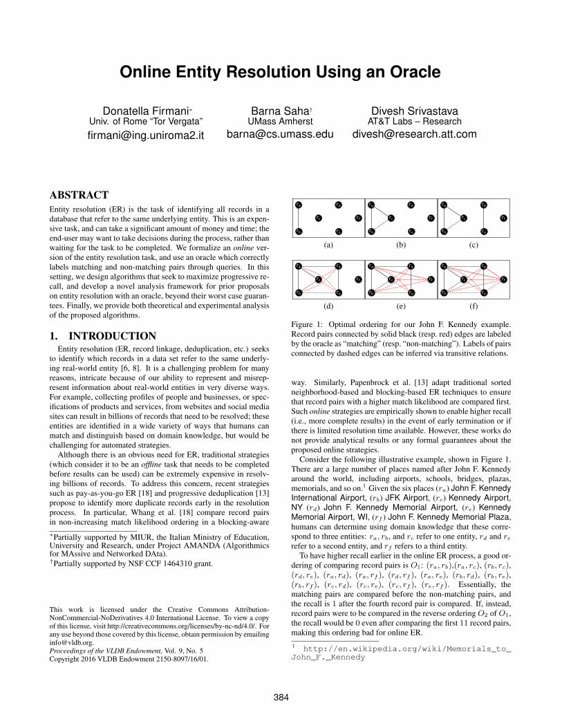
Figure 1: Optimal ordering for our John F. Kennedy example.Record pairs connected by solid black (resp. red) edges are labeledby the oracle as “matching” (resp. “non-matching”). Labels of pairsconnected by dashed edges can be inferred via transitive relations.
way. Similarly, Papenbrock et al. [13] adapt traditional sortedneighborhood-based and blocking-based ER techniques to ensurethat record pairs with a higher match likelihood are compared first.Such online strategies are empirically shown to enable higher recall(i.e., more complete results) in the event of early termination or ifthere is limited resolution time available. However, these works donot provide analytical results or any formal guarantees about theproposed online strategies.
Consider the following illustrative example, shown in Figure 1.There are a large number of places named after John F. Kennedyaround the world, including airports, schools, bridges, plazas,memorials, and so on.1 Given the six places (ra) John F. KennedyInternational Airport, (rb) JFK Airport, (rc) Kennedy Airport,NY (rd) John F. Kennedy Memorial Airport, (re) KennedyMemorial Airport, WI, (rf ) John F. Kennedy Memorial Plaza,humans can determine using domain knowledge that these corre-spond to three entities: ra, rb, and rc refer to one entity, rd and rerefer to a second entity, and rf refers to a third entity.
To have higher recall earlier in the online ER process, a good or-dering of comparing record pairs is O1: (ra, rb),(ra, rc), (rb, rc),(rd, re), (ra, rd), (ra, rf ), (rd, rf ), (ra, re), (rb, rd), (rb, re),(rb, rf ), (rc, rd), (rc, re), (rc, rf ), (re, rf ). Essentially, thematching pairs are compared before the non-matching pairs, andthe recall is 1 after the fourth record pair is compared. If, instead,record pairs were to be compared in the reverse orderingO2 ofO1,the recall would be 0 even after comparing the first 11 record pairs,making this ordering bad for online ER.
1 http://en.wikipedia.org/wiki/Memorials_to_John_F._Kennedy
384

An elegant abstraction for formally comparing offline ER strate-gies was recently studied by Wang et al. [16] and Vesdapunt etal. [14]. They propose the notion of an oracle that correctly answersquestions of the form “Do records u and v refer to the same entity?”in the context of crowdsourcing strategies, where such questionsare answered by the crowd. ER strategies are then compared interms of the total number of questions asked to an oracle to achievea recall of 1, that is, completely resolving all the records into clus-ters, each referring to a distinct real-world entity. The strategiesproposed by [16, 14] show how to make effective use of their ora-cle, and its consequence that ER satisfies the transitive relations (inwhich known match and non-match labels on some record pairs canbe used to automatically infer match or non-match labels on otherrecord pairs) to reduce the total number of questions that need to beasked of the oracle. In particular, Wang et al. [16] propose a strat-egy that asks oracle questions in non-increasing match probabil-ity ordering, while the strategy of Vesdapunt et al. [14] ask oraclequestions based on ordering records in a non-increasing orderingof expected sizes of the records’ clusters. However, minimizing thetotal number of oracle questions is not a suitable optimization ob-jective for online ER, and the strategies of [16, 14] do not alwaysperform well in the online setting.
Let us revisit our illustrative example. If we make use of thetransitive relations for ordering O1, the oracle would be asked only6 record pairs (i.e., (ra, rb), (ra, rc), (rd, re), (ra, rd), (ra, rf ),(rd, rf )), and the labels of the other 9 record pairs can be inferred.
Note that the offline ER optimization objective of minimizingthe total number of record pair queries to the oracle would alsobe achieved by considering the record pair queries to the oracle inthe following ordering O3: (ra, rd), (ra, rf ), (rd, rf ), (rd, re),(ra, rb), (ra, rc), (rb, rc), (ra, re), (rb, rd), (rb, re), (rb, rf ),(rc, rd), (rc, re), (rc, rf ), (re, rf ). Exactly the same 6 record pairqueries would be issued to the oracle as in the ordering O1. How-ever, the recall would be 0 after labeling the first three record pairs,0.25 after labeling the fourth record pair, 0.5 after labeling the fifthrecord pair, and 1.0 after labeling the sixth record pair, making O3
less suitable thanO1 for online ER. Let us assume that we have thefollowing probability estimates for record pairs2. Matching pairs:p(rd, re) = 0.80, p(rb, rc) = 0.60, p(ra, rc) = 0.54, p(ra, rb) =0.46. Non-matching pairs: p(ra, rd) = 0.84, p(rd, rf ) = 0.81,p(rc, re) = 0.72, p(ra, re) = 0.65, p(rc, rd) = 0.59, p(re, rf ) =0.59, p(ra, rf ) = 0.55, p(rb, rd) = 0.51, p(rb, re) = 0.46,p(rc, rf ) = 0.45, p(rb, rf ) = 0.29. In this case, the techniqueof Wang et al. [16] would consider pairs in the following (non-increasing ordering of probability) ordering O4: (ra, rd), (rd, rf ),(rd, re), (rc, re), (ra, re), (rb, rc), (rc, rd), (re, rf ), (ra, rf ),(ra, rc), (rb, rd), (ra, rb), (rb, re), (rc, rf ), (rb, rf ). A total of7 record pair queries would be issued to the oracle (i.e., (ra, rd),(rd, rf ), (rd, re), (rc, re), (rb, rc), (ra, rf ), (ra, rc)), which ismore than in the ordering O1. Since higher probability node pairsmay be non-matching, this is only to be expected.
The strategies proposed by [16, 14] ask one oracle question ata time. However, some applications may benefit a lot from ask-ing multiple questions in parallel. For instance, in crowd-sourcing,asking workers to execute one task at a time would not be viablein practice. To this end, Wang et al. [16] provide a parallel versionof their strategy, such that (i) questions asked do not have transitivedependence, and (ii) if the probability estimates are not too noisy,performance is similar to sequential version. This parallel strategyhas similar limitations as the sequential one in the online setting.
2We let some non-matching pairs have higher probability thanmatching pairs. Some observers, for instance, may consider ra andre more likely to be the same entity, rather than ra and rb.
1.1 ContributionsIn this paper, we formally study the problem of online ER for
an input graph, where nodes correspond to records, and edges havematch probabilities, using the oracle abstraction of [16, 14]. Wemake the following contributions.
First, we propose the use of progressive recall as the metric tobe maximized by online ER strategies. If one plots a curve of re-call (i.e., fraction of the total number of matching record pairs thathave answered as such by the oracle, or inferred) as a function ofthe number of oracle queries, progressive recall is quantified as thearea under this curve. Intuitively, progressive recall is maximizedwhen (a) the oracle is asked about matching record pairs beforebeing asked about non-matching record pairs, and (b) the oracleis asked about matching record pairs in larger clusters (i.e., enti-ties with many records) in a connected manner, before being askedabout matching record pairs in smaller clusters. The decision ver-sion of our problem is NP-complete, since it generalizes the tradi-tional optimization objective of minimizing the number of oraclequeries at the completion [14].
In our illustrative example, it is easy to verify that ordering O1
indeed maximizes progressive recall (as shown in Figure 1), con-firming our intuition that it is the best ordering for online ER.
Second, we propose a novel benefit metric, which is a robustestimate of the expected marginal gain in recall when processing apreviously unprocessed record or record pair. We present greedy al-gorithms that use this benefit metric, and build on the edge-orderingstrategy of Wang et al. [16] and the node-ordering strategy of Ves-dapunt et al. [14]. We also develop an optimized hybrid strategythat provides a significant performance improvement in practice.
Third, we propose the edge noise model based on real-worlddata, and present approximation results for the quality of the so-lutions obtained by our strategies for optimizing progressive re-call, and those by the strategies of [16, 14] for the traditional opti-mization objective and for progressive recall. The analysis of [14]showed an O(n) worst-case approximation guarantee for the algo-rithm proposed by Wang et al. [16], and an O(k) approximationguarantee for their own method, where n represents the total num-ber of records, and k represents the number of actual entities. How-ever, these worst-case behaviors are not observed in practice. Ouranalysis helps to explain this discrepancy by showing that, underthe reasonable edge noise model, the algorithms of [16, 14] havemuch better approximation guarantees. These improved approxi-mation guarantees are consistent with empirical results (see below),which show that each of these techniques does well in some cases,but does poorly in other cases.
Fourth, we do a thorough empirical comparison of our strate-gies with the strategies of Wang et al. [16], Vesdapunt et al. [14],and Papenbrock et al. [13] (which was shown to dominate the tech-niques of Whang et al. [18]) on real and synthetic datasets. We alsoimplement parallel versions of our strategies, based on the sameprinciples described in [16]. Our evaluation demonstrates the supe-riority of our hybrid strategy over the alternatives. In particular, ourhybrid strategy shows a high progressive recall on data sets with askewed distribution of entity cluster sizes (e.g., Cora bibliographydata, where the strategy of Wang et al. [16] performs poorly), andon sparse data sets (e.g., ABT-BUY Products, where the techniqueof Vesdapunt et al. [14] performs poorly). Our strategy also showsmuch higher progressive recall over large real data with blocking(DBLP data) compared to the strategy of Papenbrock et al. [13].
Our results provide the foundations for an online view of the ERtask, especially in a crowdsourcing setting, which we think is bothmore realistic and more flexible than its traditional offline view.
385

1.2 Related WorkER has a long history (see, e.g., [6, 8] for surveys), from the sem-
inal paper by Fellegi and Sunter in 1969 [7], which proposed theuse of a learning-based approach to build a classifier, to rule-basedand distance-based approaches (see, e.g., [6]), to the recently pro-posed crowdsourcing and hybrid human-machine approaches (see,e.g., [15, 10]) for this challenging task. The closest related worksto ours are the ones by Whang et al. [18] and Papenbrock et al. [13](for online ER strategies) and by Wang et al. [16] and Vesdapunt etal. [14] (for the oracle model, and use of transitivity-aware strate-gies). We have discussed these earlier in this section. Here, wepresent other closely related works, and refer the reader to priorsurveys for a detailed discussion of other strategies.Progressive recall. Progressive recall has been used by Vesdapuntet al. [14] for experimental evaluation, and by Altowim et al. [2]. Inthese works, the different approaches are compared empirically byshowing recall as a function of oracle questions or overall process-ing time, but no formal definition of progressive recall is provided.In [2], the authors also introduce a benefit function, which does nottake into account transitivity. It is worth noting that the algorithmsdescribed in [2] are based on a resolve function (which is imple-mented as a binary Naive Bayes classifier, so there is no guaranteeof correct answers) rather than our oracle abstraction.Hybrid crowdsourcing. Many frameworks have been developedto leverage humans for performing ER tasks [15, 10]. Wang etal. [15] describe a hybrid human-machine framework CrowdER,that automatically detects pairs or clusters that have a high likeli-hood of matching, which are then verified by humans. Gokhale etal. [10] proposed a hybrid approach for the end-to-end workflowof ER (including blocking and matching), making effective use ofrandom forests classifiers and active learning via human labeling.Dynamic crowdsourcing. Dynamic aspects of the crowdsourcingprocess, different than progressive recall, are tackled in [5, 17].Demartini et al. [5] dynamically generate crowdsourcing questionsto assess the results of human workers. Whang et al. [17] proposea budget-based method and explore how to make a good use oflimited resources to maximize accuracy.Oracle errors. To deal with the possibility that the crowdsourcedoracle may give wrong answers, there are simple majority votingmechanisms or more sophisticated techniques [4, 9, 11] to handlesuch errors. We do not deal with oracle errors in this paper.
1.3 OutlineThe rest of this paper is organized as follows. We formulate
our problem in Section 2, and the benefit metric in Section 3. Ouroracle-based strategies for online ER are described in Section 4.The edge noise model and our approximation results are presentedin Section 5, and our empirical evaluation is reported in Section 6.
2. PROBLEM FORMULATIONLet V = v1, . . . , vn be a set of n records. Given u, v ∈ V , we
say that u matches v when they refer to the same real-world entity.We say that a complete, edge-labeled graph C = (V,E = E+ ∪E−), is a clustering of V if C+ = (V,E+) is transitively closed,where (u, v) ∈ E+ represents that u matches with v, and (u, v) ∈E− represents that u is non-matching with v. In other words, C+
partitions V into cliques representing distinct real-world entities.We call each clique a cluster of V , and denote with c(u) the clusterof u. Let k denote the number of clusters, and c1, . . . , ck denotethe clusters in non-increasing order of size:
• the number of edges in C+ is∣∣E+
∣∣ =∑ki=1
(|ci|2
);
• the size of a spanning forest of C is n− k.
Consider an unknown clustering C, along with an oracle accessto C. Edges in C can either be asked to the oracle, or inferred –positively or negatively – leveraging transitive relations. As an ex-ample, if u matches with v, and v matches with w, then we candeduce that u matches with w without needing to ask the oracle.Similarly, if u matches with v, and v is non-matching with w, thenwe can deduce that u is non-matching with w as well. In the fol-lowing lemma, we report a prior result of Wang et al. [16].
LEMMA 1. Let T = T+ ∪ T− be a set of edges along with theoracle responses, where T+ are the edges with YES (i.e., matching)response, and T− with NO (i.e., non-matching) response.a. An edge (u, v) can be positively inferred from T+ iff there exists
a path from u to v which only consists of T+ edges.b. An edge (u, v) can be negatively inferred from T iff there exists
a path from u to v which consists of T+ edges and one T− edge.c. Any other edge cannot be inferred.
Let E+T ⊆ E+ and E−T ⊆ E− be the sets of all the edges that
can be inferred from T , positively (including edges in T+) andnegatively (including edges in T−). Let CT = (V,ET ) be thesubgraph of C induced byET . We say that CT is a T -clustering ofV . Analogously, we call each clique a T -cluster of V , and denotewith cT (u) the T -cluster of u. Given an unknown clustering C,an oracle strategy s incrementally grows a T -clustering, by askingedges to an oracle. As soon as E+
T = E+, all the informationabout matching pairs is available to the user. This requires at least∑ki=1 (|ci| − 1) = n − k questions (i.e., the size of a spanning
forest of C+), by Lemma 1. However, it can take much longer,when
∣∣E+T ∪ E
−T
∣∣ =(n2
), for the user to become aware that no
further questions are needed. This requires asking at least for onequestion (yielding a negative answer) across every pair of clustersci, cj , i 6= j. Let tr be the number of questions asked by s untilE+T = E+, and tR be the total number of questions asked by s.
Then it holds: (i) tr ≥ n− k; (ii) tR ≥ n− k +(k2
).
We refer to the above lower-bound values for tr and tR as t∗rand t∗R, respectively. The values tr and tR account for all the ques-tions, irrespective of the answer (which can be either positive ornegative). Let us now define t+r as the total number of positivequestions (that is, questions returning a positive answer) asked by sfor E+
T = E+, and let t+R be the total number of positive questionsasked by s. It follows that t+r = t+R, and that both are equal to thesize of a spanning forest of C+, i.e., n− k.Recall. As more of the cluster structure on C is revealed, the recallof s increases. We define two recall functions of s,
• recall(t) = |E+T |/|E+|, where T is the set of the first t
oracle responses, i.e., t = |T |.
• recall+(t) =∣∣∣E+
T+
∣∣∣/|E+|, where T+ is the set of the firstt positive oracle responses, i.e., t =
∣∣T+∣∣.
For any value of t, it holds recall(t) ≤ recall+(t) ≤ M ,where M is given by the following Lemma 2.
LEMMA 2. Let k′ be the biggest index in [1, k] such that∑k′
i=1(|ci| − 1) ≤ t, and let t′ be the size of a spanning for-est of c1 ∪ c2 ∪ · · · ∪ ck′ , that is t′ =
∑k′
i=1(|ci| − 1). Then,
M =∑k′
i=1 (|ci|2 )+(t−t′2 )∑k
i=1 (|ci|2 ).
PROOF. Due to transitive relations, recall+(t′) is maximizedby a strategy s′ which finds the top k′ clusters in non-increasingorder of size, yielding recall+(t′) =
∑k′i=1 (|ci|2 )/|E+|. Similarly,
386

recall+(t) is maximized by a strategy s that does like s′ afterthe first t′ questions, and then asks a spanning forest of any sized
t−t′ subgraph of ck′+1. For s, recall+(t) =∑k′
i=1 (|ci|2 )+(t−t′2 )
|E+| .
Since∣∣E+
∣∣ =∑ki=1
(|ci|2
), the bound follows.
2.1 Progressive RecallThe recall of s denotes the fraction of positive edges found,
among those of the unknown clustering C. It is the simplest mea-sure of the amount of the information that is available to the userat a given point. However, it cannot distinguish the dynamic be-haviour of different strategies. To this end, we define two progres-sive recall functions, denoting the area under the recall-questionscurves recall(t) and recall+(t).
• precall(t) =∑tt′=1 recall(t′).
• precall+(t) =∑tt′=1 recall
+(t′).
Let us consider a strategy s∗ for which precall is maximized.s∗ first grows the largest cluster c1 by asking adjacent edges be-longing to a spanning tree of c1. That is, every asked edge sharesone of its endpoints with previously asked edges. After c1 is grown,s∗ grows in sequence c2, . . . , ck in a similar fashion. Finally, s∗
asks edges in E− in any order, until all the labels are known. Af-ter the smallest cluster ck is fully grown, |T | = t∗r , E+
T = E+,recall(t) = 1 and E−T = ∅. The final phase requires
(k2
)addi-
tional questions. Therefore s∗ minimizes both tr and tR.Benefit metrics. Both progressive recall functions of a strategys can be expressed as fractions of the corresponding functions ofs∗. We refer to progressive recall of s∗ as precall∗ (for s∗,precall=precall+). We refer to such ratio functions as nor-malized progressive recall functions:
• nPrecall(t) = precall(t)precall∗(t) , in particular we define
benefit=nPrecall(t∗r).
• nPrecall+(t) = precall+(t)precall∗(t) , in particular we define
benefit+=nPrecall+(t∗r)
We choose to express benefit metrics with respect to t∗r ratherthan t∗R. Normalized progressive recall functions get closer to 1 as tgets bigger, and tR can vary up to
(n2
)on very sparse instances. In-
stead, t∗r is bounded by n. We note that benefit = 1 if and onlyif s = s∗, while a strategy different from s∗ can have benefit+
= 1 as long as the order of positive responses is the same as s∗.
2.2 Oracle problemWe are now ready to define formally our problem.
PROBLEM 1. Given a set of records V , an oracle access to C,a subset V ′ ⊆ V , and a function p(u, v) returning the probabil-ity that u and v are matching ∀u, v ∈ V ′, find the strategy thatmaximizes benefit+.
We report for comparison the problem studied in [14, 16]. Prob-lem 2 is NP-hard [14], as well as Problem 1.
PROBLEM 2. Given a set of records V , an oracle access to C,and a function p(u, v) returning the probability that u and v arematching ∀u, v ∈ V , find the strategy that minimizes tR.
LEMMA 3. Problem 1 is NP-hard.
PROOF. Problem 2 is NP-hard [14], and Problem 1 is at least ashard as Problem 2. Indeed, a strategy solving Problem 1 also solvesProblem 2, but not vice versa.
ra
rb
rc
rd
re
rf0.92
(a) be(ra, rb)
ra
rb
rc
rd
re
rfP
1.06 0.51
(b) bv(rb, P )
Figure 2: Examples of edge and node benefit values for our JohnF. Kennedy example. Colors and dashes have the same meaningas in Figure 1. The benefit of edge (ra, rb) in Figure 2a showsthat we expect to find out 2 ∗ 1 ∗ 0.46 = 0.92 positive edges, byasking (ra, rb) to the oracle. If (ra, rb) turns out to be positive (theprobability estimate of such event is p(ra, rb) = 0.46), indeed, ourcurrent result earns two new positive edges, namely (ra, rb) itself,and (rb, rc), which can be inferred using Lemma 1. In Figure 2bwe show the benefit of node rb, by setting P to the only nodes forwhich we have information stored in T , ra, rc, rd. To this end,we first compute the aggregated benefits of rb with respect to thetwo T -clusters in P , namely ra, rc and rd. Specifically, theformer shows that we expect to find out 0.46+0.60 = 1.06 positiveedges, by discovering that rb belongs to ra, rc (i.e., by asking(ra, rb) or (rb, rc) to the oracle), and the latter that we expect tofind out 0.51 positive edges, by discovering that rb belongs to rdinstead. The benefit of the node rb is finally set to the maximumaggregated benefit, i.e., 1.06.
In this paper, we consider previous and new strategies, and: (i)formally analyze their benefit+, which is affected only by theorder in which positive questions are asked; (ii) experimentallyevaluate benefit+ and benefit.
3. BENEFIT OF QUESTIONSLet us discuss what information we have a priori, when T = ∅.
As input to the considered problems, we have a (partial) functionp : V × V → [0, 1] returning the probability that u and v arematching. We can compute a function ps : V → R returning theexpected cluster size of a node v (excluding v itself).
ps(v) =∑u∈V \v
p(u, v) (1)
p can be used as the probability estimate that a non-inferableedge belongs to E+, and ps as the estimated cluster size of a nodev for which most incident edges are non-inferable.
Given a non-inferable edge (u, v), we use its probability estimatep(u, v), for computing the expected number of edges be that couldbe positively inferred if u and v are matching (including (u, v) it-self). This denotes the expected marginal gain in recall when pro-cessing the single edge (u, v).
be(u, v) = |cT (u)| ∗ |cT (v)| ∗ p(u, v) (2)
We refer to the function be as the benefit of an edge.Given a node v for which all its incident edges are non-inferable,
that is, cT (v) consists of the singleton v, we use the probabilityestimate for computing the expected number of edges bv that couldbe positively inferred (i.e., the marginal gain in recall) if any out ofa given bunch of edges incident to v, belongs to E+. Consider thebunch of edges connecting v to a set of T -clusters P.
bv(v, P ) = maxc∈CT :c6=v,c⊆P bvc(v, c) (3)bvc(v, c) = pv(v, c) ∗ |c| (4)
where pv is the probability estimate that v belongs to T -cluster c.We refer to the function bv as the benefit of a node, and to the
387
function bvc as the aggregated benefit of a node with respect to aT -cluster. In the following, we sometimes refer to the aggregatedbenefit of v with respect to cT (u), as the aggregated benefit of theedge (v, u), and use both notations bvc(v, u) and bvc(v, c), wherec = cT (u), equivalently.
For computing pv we take the mean probability of edges con-necting v to a given cluster c (which is distinct from cT (v)) as anestimate, because that is a robust estimate (and also follows as anupper bound from the Markov inequality).
pv(v, uc) =
∑u∈c p(u, v)
|c| (5)
We note that while the benefit of an edge (v, u) only considersthe estimated probability of (v, u), the aggregated benefit takes intoaccount all the probabilities of other edges (v, w), such that w ∈cT (u). Therefore all the edges (v, w), such that w ∈ cT (u) willhave the same aggregated benefit.
Recall the illustrative example from Section 1, and the probabil-ity estimates of the matching and non-matching edges. Figure 2shows the benefit of sample edges and nodes when T+ = (ra, rc)and T− = (ra, rd).
4. ORACLE STRATEGIESA strategy s for Problem 1 needs to store new responses from
the oracle, in such a way that edges that cannot be inferred as inLemma 1 can be computed efficiently, and asked to the oracle af-terwards. To this end we introduce the query(u, v) method, thatreturns the response for (u, v) from the oracle, and updates the datastructures used by a strategy accordingly. We also introduce fewauxiliaries methods, that will be used by the considered strategies:
• top-e(w) returns the top-w non-inferable edges, in non-increasing order of p.
• top-v(w) returns the top-w nodes with no incident infer-able edges, in non-increasing order of ps.
• edges(v, P ) returns an iterator over the non-inferableedges connecting a singleton cluster v to T -clusters inP ⊆ CT , in non-increasing order of p.
• edges’(v, P ) returns an iterator over the non-inferableedges connecting a singleton cluster v to T -clusters inP ⊆ CT , in non-increasing order of bvc.
In the following, we sometimes refer to the w parameter as thewindow size – or simply window – of a strategy.Complexity of update and auxiliary methods. We refer to thetotal number of operations that a strategy performs for resolv-ing V as its work. Assuming that edges that are inferable arenever asked to the oracle, the minimum work for resolving V ist∗R = (n − k) +
(k2
). For efficiently computing edges that can-
not be inferred as in Lemma 1, we use a graph data structureGS, where nodes are T -clusters and edges are non-inferable edges.Upon a positive response from the oracle we contract the corre-sponding edge, and upon a negative response we delete the cor-responding edge. During edge contraction, only one of the max-imum probability edges between two clusters survives. This re-quires O(n(n− k) + tR) work, as in the following lemma.
LEMMA 4. query method requires O(n(n− k) + tR) work.
PROOF. The fundamental operation of our algorithm is a formof edge contraction. The result of contracting the edge (u, v) isnew supernode uv. For each node w /∈ u, v, in GS, edges (w, u)
Algorithm 1 swang, described by Wang et al.
1: while V not resolved do2: (u, v)← top-e(1)3: T ← T∪ query(u, v)4: end while
Algorithm 2 svesd, described by Vesdapunt et al.
1: P ← top-v(1)2: while P 6= V do3: v ← top-v(1)4: l← edges(v, P )5: while l.next() do6: (u, v)← l.getNext()7: T ← T∪ query(u, v)8: if (u, v) ∈ E then break end if9: end while
10: P ← P ∪ v11: end while
and (w, v) are replaced by an edge (w, uv) having probability set tomaxp(w, u), p(w, v). Finally, the contracted nodes u and v withall their incident edges are removed. If the edge (w, uv) needs tobe asked, we ask to the oracle if w and the lowest-id node in the su-pernode, e.g., u, are matching3. When GS is represented using ad-jacency lists or an adjacency matrix, a single edge contraction op-eration can be implemented with a linear number of updates. Sincethe total number of edge contractions and deletions is bounded byn− k and tR respectively, the claim follows.
Using our contract/delete algorithm, top-e, edges andedges’ can be done in O(1) time. For implementing top-e, weassume that edges are sorted during a preprocessing phase in non-increasing order of p and are available in a list LE. query methodcan maintain LE updated at no additional work. edges is simplyan iterator over the adjacency list of u’s supernode. For implement-ing edges’ we need in addition an independent execution of thecontraction/delete algorithm, where probability scores of replace-ment edges upon contraction are set to mean probability of replacededges (bvc is computed as in Eq. 4). Analogously to top-e, forimplementing top-v, we assume that nodes are sorted during apreprocessing phase in non-increasing order of ps and are availablein a list LV. Upon a new response from the oracle, let (u, v) be therelative edge, LV can be maintained updated by removing nodes uand v at no additional work than query.
4.1 Prior StrategiesIn this section, we describe strategies by Wang et al. [16] and by
Vesdapunt et al. [14] in our framework. Such strategies have beendesigned as a solution to Problem 2 and we use them as a frame ofcomparison for our strategies.Wang et al. The strategy shown in Algorithm 1 selects the firstnon-inferable edge in non-increasing order of probability estimatep, and asks it to the oracle. It continues as long as there are non-inferable edges. swang does constant additional work than query.In our John F. Kennedy example (see Section 1 for pairwise proba-bility estimates), the first question made by swang is (ra, rd), whichis the edge with the highest value of p, yielding a negative answer,and then (rd, rf ), (rd, re), and so on. We notice that in real cases,negative edges may be asked before positive edges as well.Vesdapunt et al. The strategy shown in Algorithm 2 maintains aset P of “processed” nodes, having the invariant that all the edges3 Any of the endpoints of the contracted edge can be used. We usethe lowest-id node for sake of simplicity.
388

ra
rb
rc
rd
re
rfP
(a)
ra
rb
rc
rd
re
rfP
(b)
Figure 3: Example of svesd’s invariant-maintaining procedure, onthe clustering of Figure 1. Colors and dashes have the same mean-ing as in Figure 1. In the leftmost figure we show the set P afterprocessing 2 nodes. In the rightmost figure we show what happenswhen node rc is added to P : let (ra, rc) be the edge selected at line6 of Algorithm 2. When a positive response is received, the edgesconnecting rc to P can be inferred and rc is added to P .
Algorithm 3 sedge(w).
1: while V not resolved do2: W ← top-e(w)3: (u, v)← argmaxW be(u, v)4: T ← T∪ query(u, v)5: end while
connecting nodes in P have been either asked or inferred. Thestrategy selects the first node with no inferable incident edges innon-increasing order of estimated cluster size ps, and adds it to Puntil P = V . Every time a node v is selected, before adding itto P , edges connecting v and P are asked to the oracle in non-increasing order of p, until P ∪ v satisfies the invariant. Thiscan be achieved in two ways: (i) a positive response is received;(ii) all the edges connecting v andP have been asked (with negativeresponses). If (i) is the case, all the edges connecting v and P thathave not been asked can be inferred either positively or negatively(becauseP satisfies the invariant) as in Figure 3. svesd does constantadditional work than query. In our John F. Kennedy example, Pis set initially to rd, which is the node with the highest value of ps(although it belongs to the second largest cluster)4. Next selectednode is re, and the first question made by svesd is (re, rd), yielding apositive answer. P is updated to rd, re. Next selected node is ra,and the second question made by svesd is (ra, rd), which is the edgewith highest probability among those connecting ra to P , yieldinga negative answer. (ra, re) is not asked, as it can be negativelyinferred. P is updated to rd, re, ra and so on. We notice that inreal cases, expected cluster sizes may lead to a different orderingthan actual cluster sizes, as in our illustrative example.Other examples. swang and svesd executions over real dataset andactual probability estimates are shown in Section 6.3.
4.2 Strategies for Progressive RecallThe goal of the strategies described in Section 4.1 is minimizing
the total number of questions tR asked to the oracle. Hence benefitis not taken into account explicitly. Our strategies instead, as morecluster structure is revealed by the oracle, select what edge to askthe oracle as to maximize the expected marginal gain in recall.Edge ordering. The strategy shown in Algorithm 3 selects thehighest benefit edge (as in Equation 2) among the top-w non-inferable edges in non-increasing order of p. Then it asks theedge to the oracle and repeat this process until E+
T = E+ andE−T = E−. Initially, when T = ∅, all the edges have benefit equalto their probability estimate, then the first asked edge is the same as
4 Values of ps are ps(rd) = 3.55, ps(re) = 3.22, ps(ra) = 3.04,ps(rc) = 2.90, ps(rf ) = 2.69, ps(rb) = 2.32
Algorithm 4 shybrid(w, τ, θ).
1: P ← top-v(1)2: while P 6= V do3: W ← top-v(w)4: v ← argmaxW bv(v, P )5: l← edges’(v, P )6: for i = 1, b = 1; l.next() ∧ i ≤ τ ∧ b > θ; i++ do7: u← l.getNext()8: b← bvc(v, u)9: T ← T∪ query(u, v)
10: if (u, v) ∈ E then break end if11: end for12: P ← P ∪ v13: end while14: sedge(w)
in swang. As more edges of C are revealed by the oracle, however,high probability edges may have low benefit and vice versa.
For instance, let (u, v) be the highest-probability non-inferableedge at a certain point of the execution, and let u and v be singletonT -clusters. The marginal gain in recall that we would get by asking(u, v) to the oracle is ≤ 1
|E+| .If top-e(w) contains a higher benefit edge (w, z), sedge will
ask (w, z) to the oracle rather then (u, v), even though p(w, z) <p(u, v). The higher the value ofw the higher the chance that lower-probability higher-benefit edges are preferred to (u, v). If w = 1then sedge = swang.sedge does O(w (n− k)) additional work than query. Comput-
ing the benefit of edges in the window can indeed be done duringedge contraction and deletion in O(w) and O(1) additional timerespectively. If w = qn for a given constant q, sedge does asymp-totically the same work as previous strategies.
In our John F. Kennedy example, the first question made bysedge(2), is the same as swang, that is (ra, rd). As long as all the T -clusters have size 1, sedge and swang make the same choices, sincethe benefit of edges is equal to their probability estimate. After(rd, re) is asked, yielding a positive response, the highest bene-fit edge in the window (rc, re), (rb, rc) ((ra, re) can be nega-tively inferred) is still equal to the highest probability edge, that is(rc, re). After (rb, rc) is asked, the two strategies start making dif-ferent choices. swang selects (ra, rf ), and sedge(2) selects (ra, rc)(be(ra, rf ) = 0.55 and be(ra, rc) = 2∗1∗0.54 = 1.08) complet-ing cluster c1.Hybrid ordering. The strategy shown in Algorithm 4 maintainsa set P of “processed” nodes as in Algorithm 2, but no invariantis guaranteed. That is, some edges incident to nodes in P maybe non-inferable at some point. The strategy selects the highestbenefit node (as in Equation 3), among the top w nodes in V \ Pin non-increasing order of ps, and adds it to P until P = V . Everytime a node v is selected, before adding it to P , edges connecting vand P are asked to the oracle in non-increasing order of bvc, untilone of the following condition is satisfied: (i) a positive responseis received; (ii) all the edges connecting v and P have been asked(with negative responses); (iii) the benefit does not exceed a giventhreshold θ; (iv) the number of questions related to node v exceedsa given amount of trials τ . The first two conditions are the same assvesd. When P = V , non-inferable edges can still remain, whichare eventually processed using sedge(w) strategy.
If w = 1 then two extremes behaviors are possible:
• if τ = n and θ = 0 then no questions are deferred to sedge,and shybrid = svesd, except for the order in which edges in theinner loop are processed.
389

0.0001
0.001
0.01
0.1
1
0 0.1 0.2 0.3 0.4 0.5 0.6 0.7 0.8 0.9 1
frac
tion
of e
dges
probability
negativepositive
Figure 4: Probability distribution of positive (matching entities)and negative (non-matching entities) edges in cora dataset
• if τ = 0 or θ = n then all the questions are deferred to sedge,and shybrid = swang.
We set default values for θ and τ , to 0.3 and logn respectively.Computing the benefit of w nodes takes O(nw) time, and line
4 is executed n times, requiring O(n2w) additional work thanquery. If w is equal to a given constant q, shybrid does asymp-totically the same work as previous strategies and sedge.
In our John F. Kennedy example, P is set initially to rd as insvesd. Let us consider shybrid(n,n,−1), i.e., window size n, and noconstraints for trials and benefit. Differently from svesd, the nextselected node is ra, whose benefit bv(ra, P ) is 0.84, and the firstquestion is (ra, rd). P is updated to rd, ra. Next selected node isrf , whose benefit bv(rf , P ) is 0.81, and the second question madeis (rf , rd). P is updated to rd, ra, rf and so on.5.Other examples. sedge and shybrid executions over real dataset andactual probability estimates are shown in Section 6.3.
5. ANALYSIS OF STRATEGIESIn this section, we formally analyze the strategies discussed in
the previous section under a reasonable noise model. Our noisemodel closely resembles the observed noise in estimating proba-bility values in cora [12] dataset. cora is a widely used bibli-ography data set, and has been used in many prior works on ER(see, e.g., [14]). Define an indicator random variable Xu,v forevery pair of nodes u, v such that Xu,v = 1 if u and v representthe same entity, and Xu,v = 0 if u and v are different entities. Letp(u, v) denote the matching probability score between two nodesu and v. If the matching function p is perfect, then one must havep(u, v) = 1 if u and v are the same entity, that is Xu,v = 1, andp(u, v) = 0 if u and v are different entities, that is Xu,v = 0.That is Pr [Xu,v] = p(u, v). However, in the real world, matchingprobability functions are not perfect, and are corrupted by noise.To model noise in computing probability values, we define a noiseparameter ηu,v ∈ [0, 1] for every pair of nodes u, v drawn froma probability distribution Du,v . Then, p(u, v) = ηu,v if u and vrepresent different entities, that is Xu,v = 0. p(u, v) = 1− ηu,v ifu and v represent the same entity, that is Xu,v = 1. Once again weconsider Pr [Xu,v] = p(u, v). Our analysis in this paper for vari-ous algorithms is based on this edge noise model. Handling othernoise models is part of our ongoing work.
Figure 4 represents the distribution of estimated probabilities ofmatching and non-matching edges in cora data set. We see formatching edges (green), more than 70% of edges are in the range5 In this setting, as long as all the T -clusters have size 1, questionswill be asked in non-increasing order of p as in swang. The benefitof nodes is indeed equal to the maximum probability edges incidentto P . For instance when P = rd, ra, rf, the maximum benefitnode is re (bv(re, P ) = 0.80) and the maximum probability edgeincident to P is (rd, re), which has probability estimate 0.80.
of [0.7, 1], and for non-matching edges almost 95% of edges havescores between [0, 0.1]. For the rest of the matching edges below0.7, they follow a near uniform distribution. Similarly, for non-matching edges with score above 0.1, they follow a near uniformdistribution. In the analysis, we therefore assume the following dis-tributions. For matching edges, with probability
(1− α
n
), α > 0,
the score is above 0.7, and the remaining probability mass is dis-tributed uniformly in [0, 0.7). For non-matching edges, with prob-ability
(1− β
n
), β > 0, the score is below 0.1 and the remaining
probability mass is distributed uniformly in (0.1, 1]. Unif [x, y]denotes the uniform distribution in the range (x, y].
5.1 Minimizing Total Number of QuestionsIn the following, we provide approximation results for previous
strategies swang and svesd, when solving Problem 2. As discussed inSection 2, the minimum number of questions that need to be askedto the oracle, in order to identify the k clusters, is t∗R = n−k+
(k2
).
Analysis of Wang et al.’s algorithm.
THEOREM 1. swang gives an O(log2 n)-approximation algo-rithm under the edge noise model with α ≤ n
2, β = O(logn).
PROOF. Let us consider the querying process of swang, and letus fix a cluster ci whose size is at least 4 logn. At the end of theprocess, swang will ask |ci| − 1 edges from ci that form a spanningtree. Let us use STi to denote that spanning tree. Let Ri denotethe “negative” edges, i.e., belonging to E−, incident on nodes inci that are queried before all the edges in STi are queried. LetRi = (u1, x1), (u2, x2), ..., (ua, xa) for some natural numbera ≥ 0, uj ∈ ci, j = 1, 2, .., a and xj 6∈ ci, j = 1, 2, ..., a.
Consider the time when the last edge in STi is selected for query-ing. Just before that, there must be exactly 2 components of ciwhen restricted to already known edges in ci. Denote these twocomponents by c1i and c2i . The number of edges across c1i andc2i in the ground truth C is |c1i ||c2i | ≥ |ci| − 1. For any edge(s, t), s ∈ c1i , t ∈ c2i , it must hold that p(s, t) ≤ minj p(uj , xj).It must also hold that there are exactly a non-matching edges withscore higher than max(s,t)∈c1i×c
2ip(s, t).
There are overall (n − |ci|)|ci| non-matching edges incident onsome node in ci. Among them, the expected number of edges thathave values higher than 0.1 is β
n(n− |ci|)|ci| ≤ β|ci| ≤ logn|ci|.
Therefore, if the maximum value of matching edges across c1i andc2i is above 0.1, then the expected size of Ri will be less thanlogn|ci|.
On the other hand, the probability that the maximum of all thematching edges across c1i and c2i have value less than 0.1 is at most(αn
)logn ≤ 1n
.Therefore, we have
E [|Ri|] ≤ logn|ci|+1
nn|ci| = (logn+ 1)|ci|
Suppose the number of clusters of size at most 4 logn − 1 is r.The total number of negative edges with both end points in suchsmall clusters is at most 16 log2 n. Then, if tR denotes the totalnumber of questions asked to the oracle by swang strategy, we have
E [tR] ≤∑
i:|ci|≥4 logn
E [|Ri|] + 16
(r
2
)log2 n+
+
k∑i=1
(|ci| − 1) +
(k
2
)≤ O(log2 n)t∗R
390
This is in contrast to the result by Vesdapunt et al. [14], whoshowed in the worst case, Wang et al. may ask O(nt∗R) questions.They consider a very high noise level, where between two clustersof size n
2, 1
2∗ n
2
4− 1 record pairs can be misclassified as match-
ing. Under our noise model, this happens with vanishingly lowprobability. For example, consider pairs of clusters in the coradata set with the largest number of inter-cluster edges (u, v) withp(u, v) > 0.5: for a pair of clusters with sizes 55 and 149 re-spectively, swang yields 81 negative questions more than s∗ (whichneeds 1 negative question) on average over 10 runs, which is farfrom the worst case ( 55∗149
2− 1 = 4096.5) described in [14]. This
is the worst situation we found across cluster pairs in cora. For an-other pair of clusters with sizes 55 and 117 respectively, swang asks1 negative question, just like s∗. Consistently, we see this later be-havior in most cluster pairs in cora. Our analysis explains why inpractice swang is much more effective than the predicted worst caseanalysis of Vesdapunt et al.Analysis of Vesdapunt et al.’s algorithm. Vesdapunt et al. [14]provided a different algorithm: svesd estimates the cluster sizewhich contains a node v, and orders the nodes according to thatorder. At any time, the number of clusters maintained is at most k.When a node v is chosen, at most k questions are required to findout the cluster which contains v. Therefore, this gives an O(k)-approximation on the overall number of questions tR.
THEOREM 2. svesd gives an O(log2 n)-approximation algo-rithm under the edge noise model with α ≤ n
2, β = O(logn).
PROOF. Let Cv denote the true cluster size containing v, andCv =
∑u∈V p(u, v) its estimated cluster size. Let c(v) denote the
cluster that contains v.
E[Cv]
=∑u∈V
E [p(u, v)] ≈ 0.7|c(v)|+ 0.1n
This shows that Cv is a highly biased estimate of Cv and unless Cvis substantially large ω(
√n), the ordering by Cv could be arbitrary.
Therefore, even under the edge noise model, svesd may pick first knodes that belong to k different clusters. As a result
(k2
)“negative”
questions, i.e., questions resulting in a negative answer, are issued.Onward the nodes chosen must belong to one of the selected k clus-ters. Suppose the algorithm chooses a node v that belongs to clusterci. Let Rv denote the “negative” edges, i.e., belonging to E−, in-cident on node v and clusters c1, c2, .., ci−1, ci+1, ..., ck that haveprobability value higher than the highest probability value edge, inthe ground truth C, connecting v to ci. Let the highest probabilityvalue edge connecting v to ci have value 1− η. Now following thesame analysis as in Theorem 1, we get the desired approximationbound for svesd
For our application k is often Ω(n), so this gives an exponentialimprovement over the worst case guarantees of svesd analysis.
5.2 Maximizing Progressive RecallRecall from Section 2 that (i) |c1| ≥ |c2| ≥ |c3| ≥ .... ≥ |ck|;
(ii) for maximizing progressive recall the best strategy is s∗, and(iii) the minimum number of questions that need to be asked to theoracle for E+
T = E+ is t∗r = n− k.Let EOPTt be the maximum number of edges that can be pos-
itively inferred after t ≤ t∗r questions. Let Et denote the num-ber of edges that can be positively inferred after t questions. Ift =
∑ji=1 (|ci| − 1) + l where l < |cj+1| − 1, then
EOPTt =
j∑i=1
(|ci|2
)+
(l
2
)
It is tempting to use the following notion of approximation for
progressive recall: mintEOPT
tEt
However, such a measure is overlypessimistic. For example, if the first edge asked to the oracleby a strategy yields a negative answer, then E1 = 0, whereasEOPT1 = 1, and the approximation factor is unbounded. Simi-
larly, consideringEOPT
t∗rEt∗r
is also a bad measure. Assume there aren2
clusters each of size 2, then even with independent edge noisemodel, we can have n
2non-matching record pairs with probability
value higher than the probability values of the n2
matching ones.Hence, the approximation factor will be∞.
Since s∗ asks all the “positive” questions first (i.e., resulting ina positive answer), we therefore only look at the ordering of pos-itive questions under various strategies. That is, we only considert questions that result in positive answers. Let FOPTt denote themaximum number of edges that can be positively inferred after tquestions all of which result in positive answers, and let F t denotethe number of edges that can be positively inferred by an algorithmagain when all of the t questions return positive answers. Then:
benefit+ ≥ mint
FOPTt
F t
is the approximation factor of the proposed algorithm.
PROPOSITION 1. swang has an approximation factor of Ω(n)under progressive recall.
PROOF. swang algorithm can have an approximation ratio as badas O(n). Suppose C contains one big cluster of size n
3and n
3clusters each of size 2. Consider t = n
3, swang can pick n
3edges
from each of 2-sized clusters, whereas the optimum algorithm s∗
picks n3− 1 edges from the one big cluster and one edge from
one of the small clusters. Therefore, we have F t = n3
, whereasFOPTt =
(n32
).
PROPOSITION 2. svesd has an approximation factor of Ω(√n)
under progressive recall.
PROOF. Consider√n clusters each of size
√n. svesd can pick
first√n nodes each from a different cluster. After that the next√
n − 1 positive questions can correspond to a single edge fromeach of
√n− 1 different clusters. Therefore while F t =
√n− 1,
we have FOPTt =(√
n2
)= O(n).
We now focus our attention on our edge ordering methodology,sedge. The choice of w restricts the number of edges that the al-gorithm considers for computing benefit. For analysis purpose, weuse an unrestricted window size w.
PROPOSITION 3. Suppose ei1 , ei2 , ..., eik are the first edgespicked from clusters ci1 , ci2 , ..., cik respectively in the order theyare chosen by sedge. If ij = j and edge noise is chosen fromUnif(0, 1
2) then sedge achieves optimum progressive recall.
PROOF. ij = j ensures that the first edge in the ground truth Cpicked is from the largest size cluster c1. Suppose e1 = (u, v) thenif |c1| = 2, c1 is fully complete, and the algorithm behaves sameas s∗. Otherwise, |c1| > 2. Let w ∈ c1 \u, v, then the benefit ofthe edge (u,w) is 2(1− ηu,w) and the benefit of the edge (v, w) is2(1− ηv,w). Let without loss of generality, benefit of edge (u,w)be higher than (v, w), now consider any other edge that does notcontain either u or v, benefit of that edge, denoted (a, b) is 1−ηa,b.Now if 2(1 − ηu,w) ≤ 1 − ηa,b then 1 ≤ 2ηu,w − ηa,b ≤ 2ηu,w,or ηu,w ≥ 1
2which is not possible. Therefore, our sedge strategy
always picks an edge that grows the cluster c1 in a connected way,
391

exactly like s∗. Following the argument, the algorithm completesthe cluster c1, then c2, then c3 and so on giving optimum value forprogressive recall.
Note that under the Unif(0, 12) noise model, swang asks the min-
imum number of overall queries, but in terms of progressive recall,its performance could be as bad as O(n) from the best case.
The above proof relies on choosing the first edge from each clus-ter according to the non-increasing order of cluster size. However,it is possible with skewed cluster distribution that this ordering isviolated. In the worst case, sedge may choose to complete the min-imum size cluster first and so on, but every time it grows a clusterto completion, instead of giving a fragmented view. Our hybrid or-dering methodology, shybrid, is designed to avoid such a scenarioby providing a mechanism to select edges from clusters in non-increasing order of cluster size. We now analyze the shybrid strategywhere we ignore the conditions (iii) and (iv) for querying. The con-ditions (iii) and (iv) are used for the sake of optimization since ifthe benefit of a node falls below a certain threshold or more than tquestions have already resulted in negative answers then it is likelythat this node starts a new cluster.
PROPOSITION 4. Suppose E [|ci|] > E [|cj |], j > i, i, j ∈[1, k] then shybrid achieves optimum progressive recall.
This is easy to see since under this assumption, the algorithm al-ways picks all the nodes from the first cluster, then the nodes fromthe second cluster and so on. Therefore, we now consider the worstcase scenario, where the expected sizes may not reflect the true sizeand the first k nodes picked may correspond to k different clusters.
PROPOSITION 5. Suppose vi1 , vi2 , ..., vik are the “second”nodes picked from clusters ci1 , ci2 , ..., cik respectively in the or-der they are chosen by shybrid. If ij = j and edge noise is chosenfrom Unif(0, 1
2) then shybrid achieves optimum progressive recall.
The proof of the proposition is similar to Proposition 3. Essen-tially, once we have two representatives from the largest cluster, nomatter what the edge noise is, the benefit of a third node in the samecluster is higher than any other node in a different cluster and so on.Thus the algorithm first completes the first cluster, then the secondcluster and so on optimizing the progressive recall.
In the worst case, shybrid provides an O(√n)-approximation
to progressive recall. Intuitively, only the expected sizes of theclusters bigger than Θ(
√n) are preserved due to the Chernoff-
Hoeffding bound. Thus the algorithm performs close to optimalas long as clusters of size greater than Θ(
√n) are considered. Af-
ter that, if there are r clusters of size O(√n), then shybrid can grow
these clusters from the smallest size to largest in the worst scenario.If Smax and Smin are respectively the maximum and minimumsize clusters among the r clusters that is Smin ≤ Smax ≤
√n,
then the worst case approximation factor is SmaxSmin
<√n. For lack
of space, the detailed proof can be found in the full version.
6. EXPERIMENTSIn this section we discuss the results of our experiments. We
compare all the algorithms on both synthetic and real, publiclyavailable, datasets. We implemented our and prior strategies [16,14, 13] in Java, in a common framework. Edges and nodes aresorted during a preprocessing phase, and ties are broken randomly.For each strategy, we take the average recall from the same 5 inde-pendent runs of the random tie break process. We ran experimentson a machine with two CPU Intel Xeon E5520 units with 16 coreseach, running at 2.67GHz, with 16MB of cache and 64GB RAM.
dataset cora skew sqrtn prod dblp
n 1,878 900 900 2,173 3,057,838k 191 93 30 1,092 2,980,737k′ 124 93 30 1,076 54,542|c1| 236 50 30 3 159|E| 62,891 8,175 13,050 1,086 299,683t∗r 1,687 807 870 1,081 77,101ER D D D CC D
origin RR SS SS RR RS
Table 1: Number of nodes n (i.e., records), number of clustersk (i.e., entities), number of non-singleton clusters k′,size of thelargest cluster |c1|, size of the spanning forest t∗r , type of ER (dirtyor clean–clean), and origin (real or synthetic) of the data.
dataset cora skew sqrtn prod dblp
#blocks 1 1 1 1 341,280sim. Jaro [19] Ideal Ideal Jaccard Jaro [19]R 1.8M 0.4M 0.4M 2.4M 1.8Bn′ 1,878 900 900 2,173 53, 279
Table 2: Number of blocks, similarity functions, record pairs R,and n′ values. Similarity in cora and prod is computed as in [17,15]. We emphasize that the similarity function used for dblp hasno connection with the one used for the silver standard. The “ideal”function returns 1 if two records are matching and 0 otherwise.
6.1 DatasetsSome of our datasets have real attribute values and come with
their own real gold standard. We refer to such datasets as Real-Real (RR). Other datasets have synthetic attribute values and a syn-thetic gold standard (Synthetic-Synthetic, short. SS). The remain-ing dataset has real attribute values and a synthetic gold standard,that we refer to as “silver” standard (Real-Synthetic, short. RS).We compute the silver standard as in [13] (see Section 8.1 of [13]).The main properties of the datasets are listed in Table 1:
• cora [12] is a bibliography dataset. Each record containstitle, author, venue, date, and pages attributes.
• prod [1] is a product dataset of mappings from 1,081abt.com products to 1,092 buy.com products. Each recordcontains name and price attributes.
• skew and sqrtn contain fictitious hospital patients data, in-cluding name, phone number, birth date and address, that weproduced using the data set generator of the Febrl system [3].
• dblp6 is a bibliographic index on computer science articles.
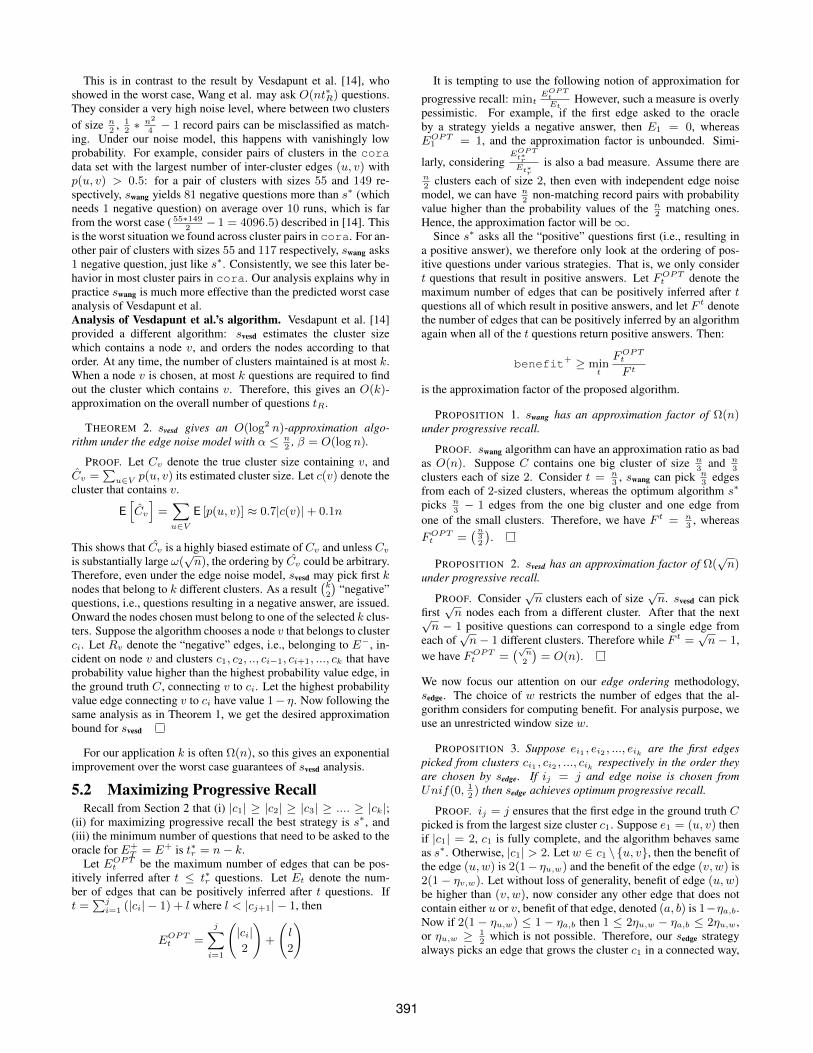
6.1.1 ClustersThe clustering graphs of cora and prod datasets, Ccora and
Cprod, are the two extremes of a spectrum. On one side, Ccora isextremely dense and few of the largest clusters account for mostrecall, thus, there is much gain in exploiting transitivity (t∗r <<∣∣E+
∣∣). On the other side, prod is extremely sparse and there isnegligible gain in exploiting transitivity (t∗r ≈
∣∣E+∣∣). (See Figure 5
for detailed visualizations.) In the middle of the spectrum:
• Cskew contains few (≈ logn) large (size ≈ nlogn
) clusters,some (≈
√n) intermediate (size ≈
√n) clusters, and a long
tail (≈ nlogn
) of small (size ≈ logn) clusters.6www.informatik.uni-trier.de/ ley/db/, 13 Aug. 2015.
392
(a) cora (b) prod
Figure 5: Clustering graphs (i.e., C) for the RR datasets. Edgecolors represent similarity scores between records (green is higher).
0.00
0.20
0.40
0.60
0.80
1.00
0.7 0.8 0.9 1
pro
babili
ty
similarity
π=1π=2log(n)/n
(a) cora
0.00
0.20
0.40
0.60
0.80
1.00
0.1 0.2 0.3 0.4 0.5 0.6 0.7 0.8 0.9 1
pro
babili
ty
similarity
π=1π=2log(n)/n
(b) prod
Figure 6: Similarity-probability mappings for the RR datasets.Record pairs with similarity values below 0.7 for cora and 0.1for prod, match with probability < 0.003. The black line showsthe identity function for comparison.
• Csqrtn contains exactly√n clusters of size
√n.
• Cdblp has skewed size distribution and is very sparse at thesame time: only 5.4× 10⁻⁶% of record pairs are duplicates.
6.1.2 ProbabilitiesWe compute edge similarities, and map them to probabilities us-
ing buckets, as in Section 3.1 of [17]. Our approach is scalable andmore general than [17]: it includes blocking, a general method forselecting bucket size, and efficient probability estimation.Blocks. Let R be the number of record pairs between which wecompute similarities. When n is large, computing all
(n2
)pairwise
similarities is not feasible. We assign records to (possibly multi-ple) blocks and compute similarities only between pairs in the sameblock. We further limit the computation to the firstO(npolylogn)pairs (which we consider feasible), by considering blocks in non-decreasing order of size. All the remaining
(n2
)− R pairs are not
submitted to the strategy, and are finally set as non-matching.
• We compute dblp blocks based on title and author tokens.We observed that log2 n is the smallest O(polylogn) func-tion which allows for including all the matching pairs whichshare at least a block, thus we set R = n log2 n.
• We consider each of other datasets as consisting of a singleblock (consistently with [17, 15]) and set R =
(n2
).
See Table 2 for details about blocking and similarity functions used.Buckets. We evenly divide the R record pairs into buckets accord-ing to their similarity and use ground truth to compute probabil-ity for each bucket. We would like many buckets in order to getenough probability values in the mapping, and at the same time,we would like large buckets in order to get a robust probability es-timate. A natural way to achieve this is byO(
√R) buckets of equal
0.10
1.00
10.00
100.00
1000.00
1 10 100
expexte
d s
ize
size
(a) cora
0.10
1.00
10.00
100.00
1000.00
1 10 100
expexte
d s
ize
size
(b) prod
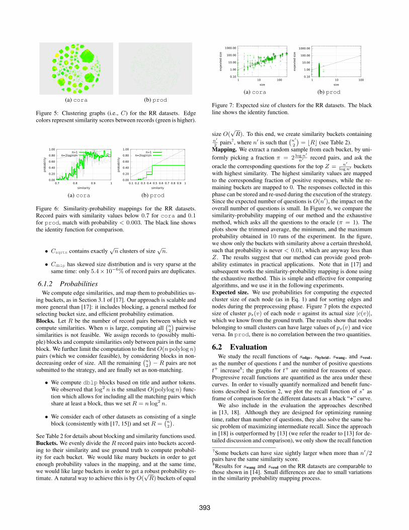
Figure 7: Expected size of clusters for the RR datasets. The blackline shows the identity function.
size O(√R). To this end, we create similarity buckets containing
n′
2pairs7, where n′ is such that
(n′
2
)= bRc (see Table 2).
Mapping. We extract a random sample from each bucket, by uni-formly picking a fraction π = 2 logn′
n′ record pairs, and ask theoracle the corresponding questions for the top Z = n′
logn′ bucketswith highest similarity. The highest similarity values are mappedto the corresponding fraction of positive responses, while the re-maining buckets are mapped to 0. The responses collected in thisphase can be stored and re-used during the execution of the strategy.Since the expected number of questions isO(n′), the impact on theoverall number of questions is small. In Figure 6, we compare thesimilarity-probability mapping of our method and the exhaustivemethod, which asks all the questions to the oracle (π = 1). Theplots show the trimmed average, the minimum, and the maximumprobability obtained in 10 runs of the experiment. In the figure,we show only the buckets with similarity above a certain threshold,such that probability is never < 0.01, which are anyway less thanZ. The results suggest that our method can provide good prob-ability estimates in practical applications. Note that in [17] andsubsequent works the similarity-probability mapping is done usingthe exhaustive method. This is simple and effective for comparingalgorithms, and we use it in the following experiments.Expected size. We use probabilities for computing the expectedcluster size of each node (as in Eq. 1) and for sorting edges andnodes during the preprocessing phase. Figure 7 plots the expectedsize of cluster ps(v) of each node v against its actual size |c(v)|,which we know from the ground truth. The results show that nodesbelonging to small clusters can have large values of ps(v) and viceversa. In prod, there is no correlation between the two quantities.
6.2 EvaluationWe study the recall functions of sedge, shybrid, swang, and svesd,
as the number of questions t and the number of positive questionst+ increase8; the graphs for t+ are omitted for reasons of space.Progressive recall functions are quantified as the area under thesecurves. In order to visually quantify normalized and benefit func-tions described in Section 2, we plot the recall function of s∗ asframe of comparison for the different datasets as a black “+” curve.
We also include in the evaluation the approaches describedin [13, 18]. Although they are designed for optimizing runningtime, rather than number of questions, they also solve the same ba-sic problem of maximizing intermediate recall. Since the approachin [18] is outperformed by [13] (we refer the reader to [13] for de-tailed discussion and comparison), we only show the recall function
7Some buckets can have size sightly larger when more than n′/2pairs have the same similarity score.8Results for swang and svesd on the RR datasets are comparable tothose shown in [14]. Small differences are due to small variationsin the similarity probability mapping process.
393
0.00
0.20
0.40
0.60
0.80
1.00
0 600 1200 1800 2400 3000 3600
reca
ll
t
w=1w=n
w=2nvesd
wangpape
(a) cora
0.00
0.20
0.40
0.60
0.80
1.00
0 300 600 900 1200 1500 1800
reca
ll
t
w=1w=nvesd
wangpape
(b) skew
0.00
0.20
0.40
0.60
0.80
1.00
0 300 600 900 1200 1500 1800
reca
ll
t
w=1w=nvesd
wangpape
(c) sqrtn
0.00
0.20
0.40
0.60
0.80
1.00
0 700 1400 2100 2800 3500 4200
reca
ll
t
w=1w=nvesd
wangpape
(d) prod
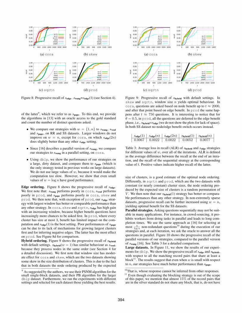
Figure 8: Progressive recall of sedge. swang=sedge(1) (see Section 4).
of the latter9, which we refer to as spape. To this end, we providethe algorithms in [13] with an oracle access to the gold standardand count the number of distinct questions asked.
• We compare our strategies with w = 1, n to swang, svesdand spape, on RR and SS datasets. Larger windows do notimprove on w = n, except for cora, on which sedge(2n)does slightly better than any other sedge setting.
• Since [16] describes a parallel version of swang, we compareour strategies to swang in a parallel setting, on cora.
• Using dblp, we show the performance of our strategies ona large, dirty dataset, and compare them to spape (which isthe only strategy tested in previous works on large datasets).We do not use large values of w, because it would make thecomputation too slow. However, we show that even smallvalues of w = log n have good performance.
Edge ordering. Figure 8 shows the progressive recall of sedge.We first note that: swang performs poorly in cora, svesd performspoorly in prod, and spape performs poorly in cora, skew andprod. We then note that, with exception of prod, our sedge strat-egy with largest window has better or comparable performance thanany other strategy. In cora, skew and sqrtn, sedge has high gainwith an increasing window, because higher benefit questions haveincreasingly more chances to be asked first. In prod, where everycluster has size at most 3, benefit has limited impact on the com-putation and sedge(1) is the best setting. Poor performances of spapecan be due to its lack of mechanisms for growing largest clustersfirst and for inferring negative edges. The latter has the most effecton prod. See Figure 8d for comparison.Hybrid ordering. Figure 9 shows the progressive recall of shybridwith default settings. shybrid(w = 1) has similar behaviour as svesd,because they process nodes in the same order (see Section 4 fora detailed discussion). We first note that window size has moder-ate effect for cora and skew, which are the two datasets showingsome skew in the size distribution of clusters. This is due to the factthat in both datasets the node ordering produced by the expected9 As suggested by the authors, we use their PSNM algorithm for thesmall single-block datasets, and their PB algorithm for the largerdblp dataset. Furthermore, we ran the experiments with differentsettings and selected for each dataset those yielding the best results.
0.00
0.20
0.40
0.60
0.80
1.00
0 600 1200 1800 2400 3000 3600
reca
ll
t
w=1w=nvesd
wangpape
(a) cora
0.00
0.20
0.40
0.60
0.80
1.00
0 300 600 900 1200 1500 1800
reca
ll
t
w=1w=nvesd
wangpape
(b) skew
0.00
0.20
0.40
0.60
0.80
1.00
0 300 600 900 1200 1500 1800
reca
ll
t
w=1w=nvesd
wangpape
(c) sqrtn
0.00
0.20
0.40
0.60
0.80
1.00
0 700 1400 2100 2800 3500 4200
reca
ll
t
w=1w=nvesd
wangpape
(d) prod
Figure 9: Progressive recall of shybrid with default settings. Inskew and sqrtn, window size n yields optimal behaviour. Incora, questions are asked based on node benefit up to t ≈ 2000,and after that point based on edge benefit. In prod the same hap-pens after t ≈ 750 questions. It is interesting to notice that forθ = 0.5, in prod, all the questions are deferred to the edge benefitphase, i.e., shybrid=sedge (we do not show the plots for lack of space).In both SS dataset no node/edge benefit switch occurs instead.
sedge(1) sedge(n) sedge(2n) shybrid(1) shybrid(n)0.0067 0.0022 0.0022 0.0052 0.0077
Table 3: Average loss in recall (ALR) of shybrid and sedge strategiesfor different values of w, over all of the iterations. ALR is definedas the average difference between the recall at the end of an itera-tion, and the recall of the sequential strategy at the correspondingvalue of t. Positive values indicate higher recall of the latter.
size of clusters, is a good estimate of the optimal node ordering.Differently, in sqrtn and prod, which are the two datasets withconstant (or nearly constant) cluster sizes, the node ordering pro-duced by the expected size of clusters is a random permutation ofV . We then note that our shybrid(1) strategy has better or compara-ble performances than any other strategy. In non-extremely sparsedatasets, progressive recall can be further increased using w = n,yielding optimal benefit for the SS datasets.Parallel strategies. Asking questions sequentially may not be suit-able in many applications. For instance, in crowd-sourcing, it pro-hibits workers from doing tasks in parallel and leads to long com-pletion times. We use the same approach as [16] for selecting atmost n
lognnon-redundant questions10 during the execution of our
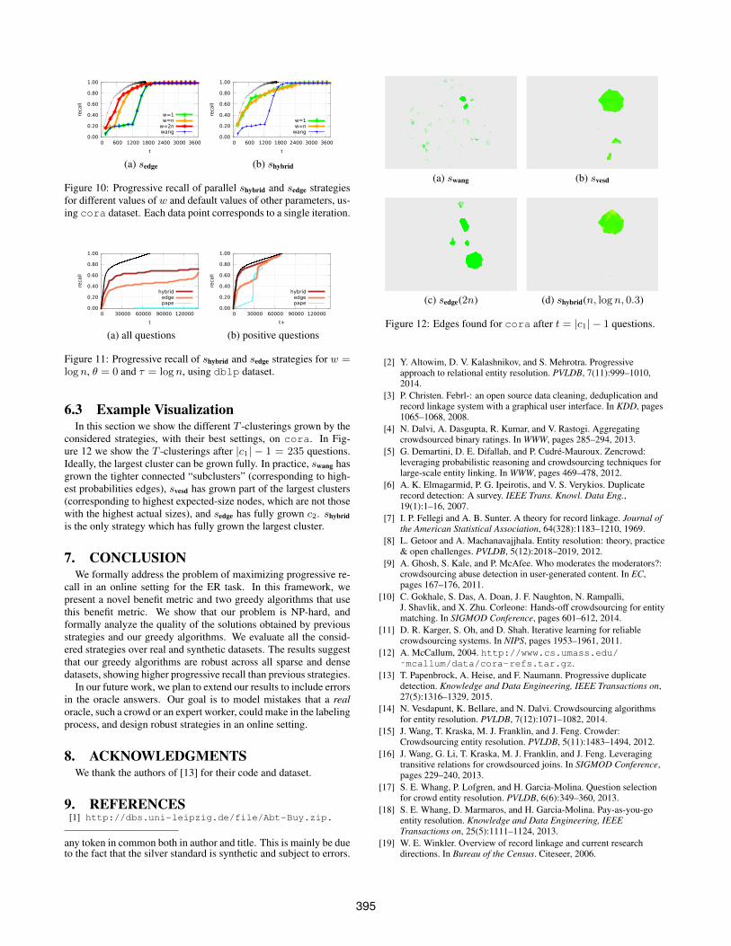
strategies and, at each iteration, we ask the oracle to answer all thequestions in parallel. Figure 10 shows the progressive recall of theparallel versions of our strategies, compared to the parallel versionof swang [16]. See Table 3 for a detailed comparison.Large datasets. In Figure 11, we show the results of our experi-ments for dblp. We show the progressive recall of sedge and shybrid,with respect to all the matching record pairs that share at least ablock11. The results suggest that even when w is small with respectto n, our strategies have much better performance than spape.
10That is, whose response cannot be inferred from other responses.11 Even though evaluating the blocking strategy is out of the scopeof this paper, we mention that almost 15% of the record pairs thatare in the silver standard do not share any block, that is, do not have
394
0.00
0.20
0.40
0.60
0.80
1.00
0 600 1200 1800 2400 3000 3600
reca
ll
t
w=1w=n
w=2nwang
(a) sedge
0.00
0.20
0.40
0.60
0.80
1.00
0 600 1200 1800 2400 3000 3600
reca
ll
t
w=1w=n
wang
(b) shybrid
Figure 10: Progressive recall of parallel shybrid and sedge strategiesfor different values of w and default values of other parameters, us-ing cora dataset. Each data point corresponds to a single iteration.
0.00
0.20
0.40
0.60
0.80
1.00
0 30000 60000 90000 120000
reca
ll
t
hybridedgepape
(a) all questions
0.00
0.20
0.40
0.60
0.80
1.00
0 30000 60000 90000 120000
reca
ll
t+
hybridedgepape
(b) positive questions
Figure 11: Progressive recall of shybrid and sedge strategies for w =logn, θ = 0 and τ = log n, using dblp dataset.
6.3 Example VisualizationIn this section we show the different T -clusterings grown by the
considered strategies, with their best settings, on cora. In Fig-ure 12 we show the T -clusterings after |c1| − 1 = 235 questions.Ideally, the largest cluster can be grown fully. In practice, swang hasgrown the tighter connected “subclusters” (corresponding to high-est probabilities edges), svesd has grown part of the largest clusters(corresponding to highest expected-size nodes, which are not thosewith the highest actual sizes), and sedge has fully grown c2. shybridis the only strategy which has fully grown the largest cluster.
7. CONCLUSIONWe formally address the problem of maximizing progressive re-
call in an online setting for the ER task. In this framework, wepresent a novel benefit metric and two greedy algorithms that usethis benefit metric. We show that our problem is NP-hard, andformally analyze the quality of the solutions obtained by previousstrategies and our greedy algorithms. We evaluate all the consid-ered strategies over real and synthetic datasets. The results suggestthat our greedy algorithms are robust across all sparse and densedatasets, showing higher progressive recall than previous strategies.
In our future work, we plan to extend our results to include errorsin the oracle answers. Our goal is to model mistakes that a realoracle, such a crowd or an expert worker, could make in the labelingprocess, and design robust strategies in an online setting.
8. ACKNOWLEDGMENTSWe thank the authors of [13] for their code and dataset.
9. REFERENCES[1] http://dbs.uni-leipzig.de/file/Abt-Buy.zip.
any token in common both in author and title. This is mainly be dueto the fact that the silver standard is synthetic and subject to errors.
(a) swang (b) svesd
(c) sedge(2n) (d) shybrid(n, logn, 0.3)
Figure 12: Edges found for cora after t = |c1| − 1 questions.
[2] Y. Altowim, D. V. Kalashnikov, and S. Mehrotra. Progressiveapproach to relational entity resolution. PVLDB, 7(11):999–1010,2014.
[3] P. Christen. Febrl-: an open source data cleaning, deduplication andrecord linkage system with a graphical user interface. In KDD, pages1065–1068, 2008.
[4] N. Dalvi, A. Dasgupta, R. Kumar, and V. Rastogi. Aggregatingcrowdsourced binary ratings. In WWW, pages 285–294, 2013.
[5] G. Demartini, D. E. Difallah, and P. Cudre-Mauroux. Zencrowd:leveraging probabilistic reasoning and crowdsourcing techniques forlarge-scale entity linking. In WWW, pages 469–478, 2012.
[6] A. K. Elmagarmid, P. G. Ipeirotis, and V. S. Verykios. Duplicaterecord detection: A survey. IEEE Trans. Knowl. Data Eng.,19(1):1–16, 2007.
[7] I. P. Fellegi and A. B. Sunter. A theory for record linkage. Journal ofthe American Statistical Association, 64(328):1183–1210, 1969.
[8] L. Getoor and A. Machanavajjhala. Entity resolution: theory, practice& open challenges. PVLDB, 5(12):2018–2019, 2012.
[9] A. Ghosh, S. Kale, and P. McAfee. Who moderates the moderators?:crowdsourcing abuse detection in user-generated content. In EC,pages 167–176, 2011.
[10] C. Gokhale, S. Das, A. Doan, J. F. Naughton, N. Rampalli,J. Shavlik, and X. Zhu. Corleone: Hands-off crowdsourcing for entitymatching. In SIGMOD Conference, pages 601–612, 2014.
[11] D. R. Karger, S. Oh, and D. Shah. Iterative learning for reliablecrowdsourcing systems. In NIPS, pages 1953–1961, 2011.
[12] A. McCallum, 2004. http://www.cs.umass.edu/˜mcallum/data/cora-refs.tar.gz.
[13] T. Papenbrock, A. Heise, and F. Naumann. Progressive duplicatedetection. Knowledge and Data Engineering, IEEE Transactions on,27(5):1316–1329, 2015.
[14] N. Vesdapunt, K. Bellare, and N. Dalvi. Crowdsourcing algorithmsfor entity resolution. PVLDB, 7(12):1071–1082, 2014.
[15] J. Wang, T. Kraska, M. J. Franklin, and J. Feng. Crowder:Crowdsourcing entity resolution. PVLDB, 5(11):1483–1494, 2012.
[16] J. Wang, G. Li, T. Kraska, M. J. Franklin, and J. Feng. Leveragingtransitive relations for crowdsourced joins. In SIGMOD Conference,pages 229–240, 2013.
[17] S. E. Whang, P. Lofgren, and H. Garcia-Molina. Question selectionfor crowd entity resolution. PVLDB, 6(6):349–360, 2013.
[18] S. E. Whang, D. Marmaros, and H. Garcia-Molina. Pay-as-you-goentity resolution. Knowledge and Data Engineering, IEEETransactions on, 25(5):1111–1124, 2013.
[19] W. E. Winkler. Overview of record linkage and current researchdirections. In Bureau of the Census. Citeseer, 2006.
395