Online Appendix for “Subways and Urban Air Pollution” by Gendron-Carrier,Gonzalez-Navarro, Polloni and Turner

A AOD data

Figure A.1: modis Terra and Aqua AOD data

#C

itie

sw

ith

AO

D6=

φ0

1530

4560

2000m1 2004m1 2008m1 2012m1 2016m1M

ean

AO

D,1

0km

disk

s.3

.4.5

.6.7

2000m1 2004m1 2008m1 2012m1 2016m1

(a) (b)

Note: Panel (a) gives count of new subway cities in our primary estimation sample with non-missing AOD10km measurements by month for Terra (dashed black) and Aqua (gray). Panel (b) shows mean AOD within10km of the center of subway cities, averaged over cities, by month for Terra (dashed black) and Aqua (gray).

The Moderate Resolution Imaging Spectroradiometers (MODIS) aboard the Terra and AquaEarth observing satellites measure the ambient aerosol optical depth (AOD) of the atmosphere al-most globally. We use MODIS Level-2 daily AOD products from Terra for February 2000-December2017 and Aqua for July 2002-December 2017 to construct monthly average AOD levels in cities. Wedownload all the files from the NASA File Transfer Protocol.1

There are four MODIS Aerosol data product files: MOD04_L2 and MOD04_3K, containingdata collected from the Terra platform; and MYD04_L2 and MYD04_3K, containing data collectedfrom the Aqua platform. We use products MOD04_3K and MYD04_3K to get AOD measuresat a spatial resolution (pixel size) of approximately 3 x 3 kilometers. Each product file covers afive-minute time interval based on the start time of each MODIS granule. The product files arestored in Hierarchical Data Format (HDF) and we use the "Optical Depth Land And Ocean" layer,which is stored as a Scientific Data Set (SDS) within the HDF file, as our measure of aerosol opticaldepth. The "Optical Depth Land And Ocean" dataset contains only the AOD retrievals of highquality.

We convert all HDF formatted granules to GIS compatible formats using the HDF-EOS ToGeoTIFF Conversion Tool (HEG) provided by NASA’s Earth Observing System Program.2 Weconsolidate GeoTIFF granules into a global raster for each day using ArcGIS. First, we keep onlyAOD values that do contain information. The missing value is -9999 in AOD retrievals. Second,we create a raster catalog with all the granules for a given day and calculate the average AODvalue using the Raster Catalog to Raster Dataset tool.

1ftp://ladsweb.nascom.nasa.gov/allData/6/2The most recent version of the software, HEG Stand-alone v2.13, can be downloaded at

http://newsroom.gsfc.nasa.gov/sdptoolkit/HEG/HEGDownload.html

1

Figure A.1 provides more information about the coverage of the two satellites and the preva-lence of missing data. The black dashed line in panel (a) of the figure gives the count of cities inour primary estimation sample for which we calculate an AOD from the Terra satellite readingfor each month of our study period. These are cities for which there is at least one pixel within10km of the center on one day during the relevant month. Since most of the cities in our data arein the Northern hemisphere, we see a strong seasonal pattern in this series. The light gray linein this figure reports the corresponding quantity calculated from the Aqua satellite reading. SinceAqua became operational after Terra, the Aqua series begins later. The Aqua satellite data tracksthe Terra data closely, but at a slightly lower level. Panel (b) of Figure A.1 reports city mean AODdata for all city-months in our sample over the course of our study period. As for the other series,this one too exhibits seasonality, although this will partly reflect a composition effect. As we seein panel (a) not all cities are in the data for all months. As in the first two panels, the dark linedescribes AOD readings from Terra and the light gray, Aqua.

B Ridership data

We gathered subway ridership data (unlinked trips) for 42 of the subway systems in our mainestimating sample, mostly from annual reports or statistical agencies. In 16 cases we were eithernot able to find data on ridership at all, the data were not available from the opening date, or theridership data was aggregated across cities or other rail systems. Data sources for each of the citieswe were able to obtain usable data are detailed in Table A.1.

2

Table A.1: Ridership Data Sources

City Source & URL Date accessedAlmaty (Kazakhstan) International Metro Association reports Feb. 2020

http://eng.asmetro.ru/metro/techno_ekonom/

Bangalore (India) Bangalore Metro operational performance reports Feb. 2020

https://kannada.bmrc.co.in/English/rti.html

Brescia (Italy) Brescia Mobilitá reports Feb. 2020

https://www.comune.brescia.itChangsha (China) China Association of Metros annual reports Feb. 2020

https://www.camet.org.cn/tjxx/3101

Chennai (India) Chennai Metro Rail Limited annual reports Feb. 2020

https://chennaimetrorail.orgCopenhagen (Denmark) Statistics Denmark Feb. 2020

https://www.statbank.dk/bane21

Daejeon (South Korea) Daejeon Metropolitan Rapid Transit Corporation Feb. 2020

http://info.korail.com/common/downLoad.mbs?fileSeq=14648002&boardId=9863289

Delhi (India) Delhi Metro Rail Corporation annual reports Feb. 2020

http://www.delhimetrorail.com/annual_report.aspx

Dongguan (China) China Association of Metros annual reports Feb. 2020

https://www.camet.org.cn/tjxx/3101

Dubai (UAE) Dubai Road and Transport Auth.: Annual statistical reports Feb. 2020

https://www.dsc.gov.ae/Report/Copy%20of%20DSC_SYB_2016_11%20_%2011.xlsx

Fuzhou (China) China Association of Metros annual reports Feb. 2020

https://www.camet.org.cn/tjxx/3101

Gwangju (South Korea) Gwangju Subway reports Feb. 2020

http://info.korail.com/common/downLoad.mbs?fileSeq=14648002&boardId=9863289

Hangzhou (China) Hangzhou Statistical Yearbook Feb. 2020

Continued on next page

3

Table A.1 – continued from previous pageCity Source & URL Date accessed

https://www.camet.org.cn/tjxx/3101

Harbin (China) China Association of Metros annual reports Feb. 2020

https://www.camet.org.cn/tjxx/3101

Jaipur (India) Jaipur Metro annual reports Feb. 2020

https://transport.rajasthan.gov.in/jmrc/Kazan (Russia) International Metro Association reports Feb. 2020

http://eng.asmetro.ru/metro/techno_ekonom/

Kaohsiung (Taiwan) Kaohsiung Rapid Transit Corp. transport volume statistics Feb. 2020

https://corp.krtc.com.tw/eng/News/annual_report

Lausanne (Switzerland) Transports Lausanne Annual Reports Feb.2020

http://app.iqr.ch/rapportactivite2015

Lima (Peru) Ministerio de Transportes y Comunicaciones Perú Feb.2020

https://portal.mtc.gob.pe/estadisticas Feb.2020

Mashhad (Iran) Mashhad Urban Railway Corp. planning and development Feb. 2020

http://metro.mashhad.ir/Mumbai (India) Mumbai Metro One Pvt. Ltd. right to information request Feb. 2020

http://www.reliancemumbaimetro.com

Nanning (China) China Association of Metros annual reports Feb. 2020

https://www.camet.org.cn/tjxx/3101

Naha (Japan) Okinawa Ciy Monorail Line (Yui Rail) Feb. 2020

https://www.yui-rail.co.jp/yuirail/past-users/

Nanchang (China) China Association of Metros annual reports Feb. 2020

https://www.camet.org.cn/tjxx/3101

Ningbo (China) China Association of Metros annual reports Feb. 2020

https://www.camet.org.cn/tjxx/3101

Continued on next page

4

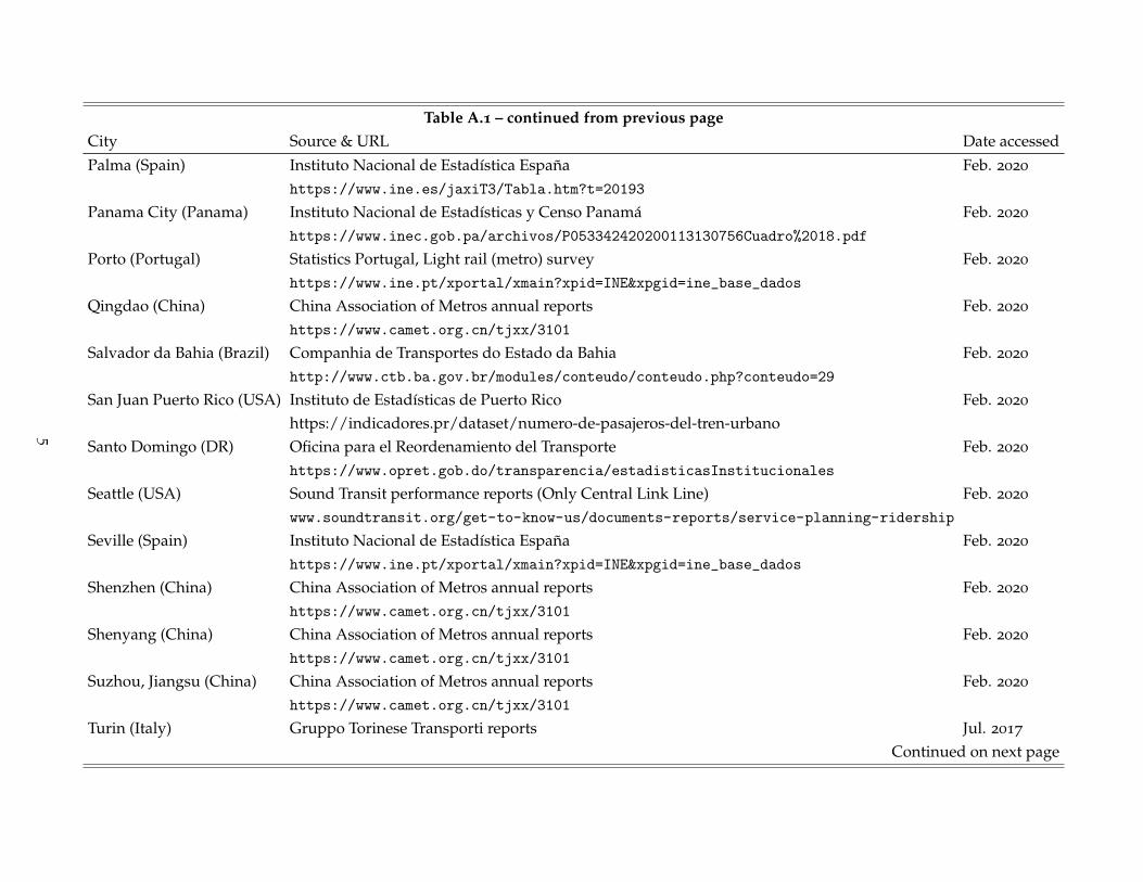
Table A.1 – continued from previous pageCity Source & URL Date accessedPalma (Spain) Instituto Nacional de Estadística España Feb. 2020

https://www.ine.es/jaxiT3/Tabla.htm?t=20193

Panama City (Panama) Instituto Nacional de Estadísticas y Censo Panamá Feb. 2020

https://www.inec.gob.pa/archivos/P053342420200113130756Cuadro%2018.pdf

Porto (Portugal) Statistics Portugal, Light rail (metro) survey Feb. 2020

https://www.ine.pt/xportal/xmain?xpid=INE&xpgid=ine_base_dados

Qingdao (China) China Association of Metros annual reports Feb. 2020

https://www.camet.org.cn/tjxx/3101

Salvador da Bahia (Brazil) Companhia de Transportes do Estado da Bahia Feb. 2020

http://www.ctb.ba.gov.br/modules/conteudo/conteudo.php?conteudo=29

San Juan Puerto Rico (USA) Instituto de Estadísticas de Puerto Rico Feb. 2020

https://indicadores.pr/dataset/numero-de-pasajeros-del-tren-urbanoSanto Domingo (DR) Oficina para el Reordenamiento del Transporte Feb. 2020

https://www.opret.gob.do/transparencia/estadisticasInstitucionales

Seattle (USA) Sound Transit performance reports (Only Central Link Line) Feb. 2020

www.soundtransit.org/get-to-know-us/documents-reports/service-planning-ridership

Seville (Spain) Instituto Nacional de Estadística España Feb. 2020

https://www.ine.pt/xportal/xmain?xpid=INE&xpgid=ine_base_dados

Shenzhen (China) China Association of Metros annual reports Feb. 2020

https://www.camet.org.cn/tjxx/3101

Shenyang (China) China Association of Metros annual reports Feb. 2020

https://www.camet.org.cn/tjxx/3101

Suzhou, Jiangsu (China) China Association of Metros annual reports Feb. 2020

https://www.camet.org.cn/tjxx/3101

Turin (Italy) Gruppo Torinese Transporti reports Jul. 2017

Continued on next page

5

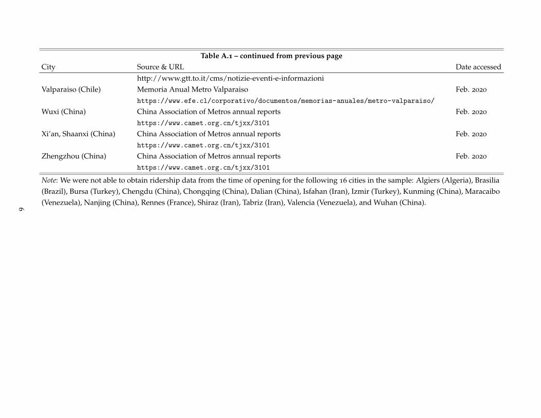
Table A.1 – continued from previous pageCity Source & URL Date accessed

http://www.gtt.to.it/cms/notizie-eventi-e-informazioniValparaiso (Chile) Memoria Anual Metro Valparaiso Feb. 2020

https://www.efe.cl/corporativo/documentos/memorias-anuales/metro-valparaiso/

Wuxi (China) China Association of Metros annual reports Feb. 2020

https://www.camet.org.cn/tjxx/3101

Xi’an, Shaanxi (China) China Association of Metros annual reports Feb. 2020

https://www.camet.org.cn/tjxx/3101

Zhengzhou (China) China Association of Metros annual reports Feb. 2020

https://www.camet.org.cn/tjxx/3101

Note: We were not able to obtain ridership data from the time of opening for the following 16 cities in the sample: Algiers (Algeria), Brasilia(Brazil), Bursa (Turkey), Chengdu (China), Chongqing (China), Dalian (China), Isfahan (Iran), Izmir (Turkey), Kunming (China), Maracaibo(Venezuela), Nanjing (China), Rennes (France), Shiraz (Iran), Tabriz (Iran), Valencia (Venezuela), and Wuhan (China).

6

C AOD vs ground based measurements

Table A.2: Relationship between AOD and Ground-based Particulate Measures

PM10 PM2.5

(1) (2) (3) (4) (5) (6) (7) (8)AOD 135.8 114.6 118.1 113.0 101.7 103.3 76.6 60.6

(9.7) (11.8) (11.5) (11.9) (10.0) (10.9) (6.7) (8.3)cons 4.5 134.5 110.7 136.9 136.6 140.0 -0.5 19.9

(2.8) (39.3) (39.8) (39.5) (41.1) (42.3) (1.5) (27.5)Mean dep. var. 57.25 57.25 57.25 57.25 57.35 57.35 23.72 23.72Mean ind. var. 0.39 0.39 0.36 0.39 0.37 0.39 0.32 0.32R2 0.50 0.82 0.81 0.82 0.83 0.82 0.61 0.85N 340 340 340 340 339 339 217 217

Note: (1) Terra 10k disk, no controls. (2) Terra 10k disk, controls. (3) Aqua 10k disk, controls. (4) Terra10k footprint, controls. (5) Terra 25k disk, controls. (6) Terra 25k footprint, controls. (7) Terra 10k disk,no controls. (8) Terra 10k disk, controls. Controls: continent-year indicators, average pixel count, andlinear and quadratic terms in average temperature, precipitation, cloud cover, vapor pressure and frost days.Robust standard errors in parentheses.

Figure A.2: AOD versus PM

-50

050

100

150

200

-.4 -.2 0 .2 .4

0.0

1.0

2.0

3.0

4.0

5Fr

actio

n

0 10 20 30 40 50 60 70 80 90 100 110 120PM2.5

0 20 40 60 80 100 120 140 160 180 200 220PM10

0 .2 .4 .6 .8 1 1.2 1.4 1.6AOD

(a) (b)

Note: (a) Plot showing residualized PM10 and AOD, together with linear trend. (b) Histogram of city-months by AOD, pm10 and pm2.5 . pm10 and pm2.5 axes rescaled from AOD using columns 1 and 4 ofTable A.2. Black vertical line indicates WHO threshold level for annual average pm10 exposure (WHO,2006).

A series of papers have compared measures of AOD to measures of particulate concentrationfrom surface instruments (e.g. Gupta, Christopher, Wang, Gehrig, Lee, and Kumar, 2006, Kumar,

7

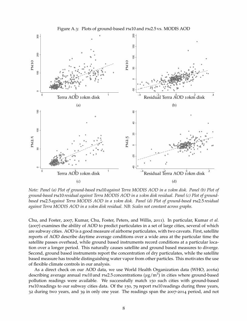
Figure A.3: Plots of ground-based pm10 and pm2.5 vs. MODIS AODpm

10

010

020

030

0

0 .5 1

pm

10

-50

050

100

150

200

-.4 -.2 0 .2 .4Terra AOD 10km disk Residual Terra AOD 10km disk

(a) (b)

pm

2.5

050

100

150

0 .5 1

pm

2.5

-40

-20

020

4060

-.4 -.2 0 .2Terra AOD 10km disk Residual Terra AOD 10km disk

(c) (d)

Note: Panel (a) Plot of ground-based pm10 against Terra MODIS AOD in a 10km disk. Panel (b) Plot ofground-based pm10 residual against Terra MODIS AOD in a 10km disk residual. Panel (c) Plot of ground-based pm2.5 against Terra MODIS AOD in a 10km disk. Panel (d) Plot of ground-based pm2.5 residualagainst Terra MODIS AOD in a 10km disk residual. NB: Scales not constant across graphs.

Chu, and Foster, 2007, Kumar, Chu, Foster, Peters, and Willis, 2011). In particular, Kumar et al.(2007) examines the ability of AOD to predict particulates in a set of large cities, several of whichare subway cities. AOD is a good measure of airborne particulates, with two caveats. First, satellitereports of AOD describe daytime average conditions over a wide area at the particular time thesatellite passes overhead, while ground based instruments record conditions at a particular loca-tion over a longer period. This naturally causes satellite and ground based measures to diverge.Second, ground based instruments report the concentration of dry particulates, while the satellitebased measure has trouble distinguishing water vapor from other particles. This motivates the useof flexible climate controls in our analysis.

As a direct check on our AOD data, we use World Health Organization data (WHO, 2016a)describing average annual pm10 and pm2.5 concentrations (µg/m3) in cities where ground-basedpollution readings were available. We successfully match 150 such cities with ground-basedpm10 readings to our subway cities data. Of the 150, 79 report pm10 readings during three years,32 during two years, and 39 in only one year. The readings span the 2007-2014 period, and not

8

all city-years record both pm10 and pm2.5 . Averaging monthly AOD values to calculate yearlyaverages, we obtain 340 comparable city-years for pm10 and 217 comparable city-years for pm2.5 .Note the limited amount of data available from ground-based instruments. Satellite data solvethe issue of data scarcity. In particular, not that the ground based measurements are annual, asopposed to the monthly data we use elsewhere.

To compare the WHO ground-based annual measures of particulates to annual averages ofMODIS AOD measurements in subway cities, we estimate the following regressions

PMyit = α0 + α1AODit + controlsit + εit,

where y ∈ {2.5,10} is particulate size, i refers to cities and t to years for which we can match who

data to our AOD sample.Table A.2 reports results. The upper first column presents the results of a regression of the WHO

measure of pm10 on annual average Terra AOD within 10km of a subway city center. There is astrong positive relationship between the two quantities and the R2 of the regression is 0.50. TheAOD coefficient of 135.81 in Column 1 means that a one unit increase in AOD maps to a 135.81

µg/m3 increase in pm10 . From Table 1 in the paper, we see that Terra 10k readings for NorthAmerica decreased by 0.03 in subway cities between 2000 and 2017. Multiplying by 135.81 gives a4.1µg3 decrease in PM10. By contrast, according to US EPA historical data, during this same periodUS average pm10 declined from 64.7 to 57.7 µg/m3, or about a 7 unit decrease.3 Since Table 1 in thepaper reports AOD for just the three cities in North America with new subways, while the EPAreports area weighted measures for the US, this seems as close as could be expected.

In Column 2, we conduct the same regression but include linear and quadratic terms in ourclimate variables, average pixel count, and continent-year indicators. The coefficient on AODdrops from 135.81 to 114.60, and the R2 increases to 0.82. In Column 3, we conduct exactly thesame regression, but rely on AOD measurements from the Aqua satelite. As expected this leavesour estimates qualitatively unchanged.

Columns (4)-(6) repeat (2) but use different geographies to construct the AOD measure. InColumn (4) we measure AOD in the intersection of the lights based city footprint and a 10kmdisk centered on the city. In Column (5) we measure AOD in a 25km disk centered on the city.In Column (6) we measure AOD in the intersection of the lights based footprint and the 25kmdisk. Coefficients vary slightly over the different specifications, but R2s do not. In theory, thissequence of regressions could have revealed that ground based instruments are more closelyrelated to a particular AOD measure. In fact, this seems not to be the case. Thus, the comparison ofremotely sensed and ground based measures does not suggest that footprints are to be preferred todisks for the analysis based on R2s. Given this, and given that most subway systems concentratetheir service in the center part of the city (Gonzalez-Navarro and Turner, 2018), we rely on AODcalculated of centrally located 10km disks for our main analysis.

For completeness, columns (7) and (8) replicate columns (1) and (2), but use ground basedmeasures of PM2.5 as the dependent variable. Since PM2.5 comprises a smaller fraction of allairborne particulates than does PM10, the smaller coefficients in these regressions is expected.In fact, the AOD coefficient for PM2.5 from Column (8) is about 53% of the one for PM10 inColumn (2). This is consistent with the pm10 to pm2.5 conversion factors used by the World HealthOrganisation (WHO, 2016a).4

All specifications reported in Table A.2 assume a linear relationship between AOD and PM.Figure A.2(a) plots residuals of regressions of PM10 and AOD on all controls used in Column 2

3https://www.epa.gov/air-trends/particulate-matter-pm10-trends, accessed July 2, 2020.4We note that the results in Table A.2 are quite different from those on which the 2013 Global burden of disease

estimates are based (Brauer et al. 2015). In particular, they estimate

ln(pm2.5 ) ≈ 0.8 + 0.7 ln(AOD).

9

of Table A.2, along with a linear regression line. This graph illustrates both how closely the twovariables track each other and how close to linear is the relationship between them.

Recall that the ground-based instruments and MODIS, in fact, measure something different.Ground-based instruments measure pollution at a point over an extended period of time. Remotesensing measures particulates across a wide area at an instant. Given this difference, the extent towhich the two measures agree seems remarkable.

In addition to validating the use of remotely sensed AOD, Table A.2 provides a basis for trans-lating our estimates of the relationship between subways and AOD into a relationship betweensubways and pm2.5 , or pm10 . To illustrate this process, and to help to describe our data, FigureA.2(b) provides a histogram of the 21,806 city-months used for our main econometric analysis. Thefigure provides three different scales for the horizontal axis. The top scale is the raw AOD measure.The second two axes are affine transformations of the AOD scale into pm10 and pm2.5 based oncolumns (1) and (7) of Table A.2. For reference, the black line in the figure gives the World HealthOrganization recommended maximum annual average pm10 exposure level (20 µg/m3).

D Global Burden of Disease based mortality estimates

The integrated risk functions in Burnett et al. (2014) express the likelihood of dying from a disease atcurrent pm2.5 exposure, relative to an environment where pm2.5 concentrations are set to a baselineharmless level of exposure. If Dd is the event of dying from disease d, the risk ratio (RR) of beingexposed to pm2.5 concentration c is given by RRd(c, c̄) = P(Dd | c)/P(Dd | c̄), where c̄ denotesthe baseline harmless concentration. Burnett et al. (2014) model RRd(c, c̄) to exhibit diminishingmarginal risk: RR(c,c̄) = 1 + α(1 − e−γ(c−c̄)δ

) if c > c̄ , and RR(c,c̄) = 1 otherwise, with c̄assumed to lie uniformly between 5.8 and 8.8µg/m3. We refer the reader to Burnett et al. (2014) fordetails regarding the parametrization and estimation of these functions for each disease.

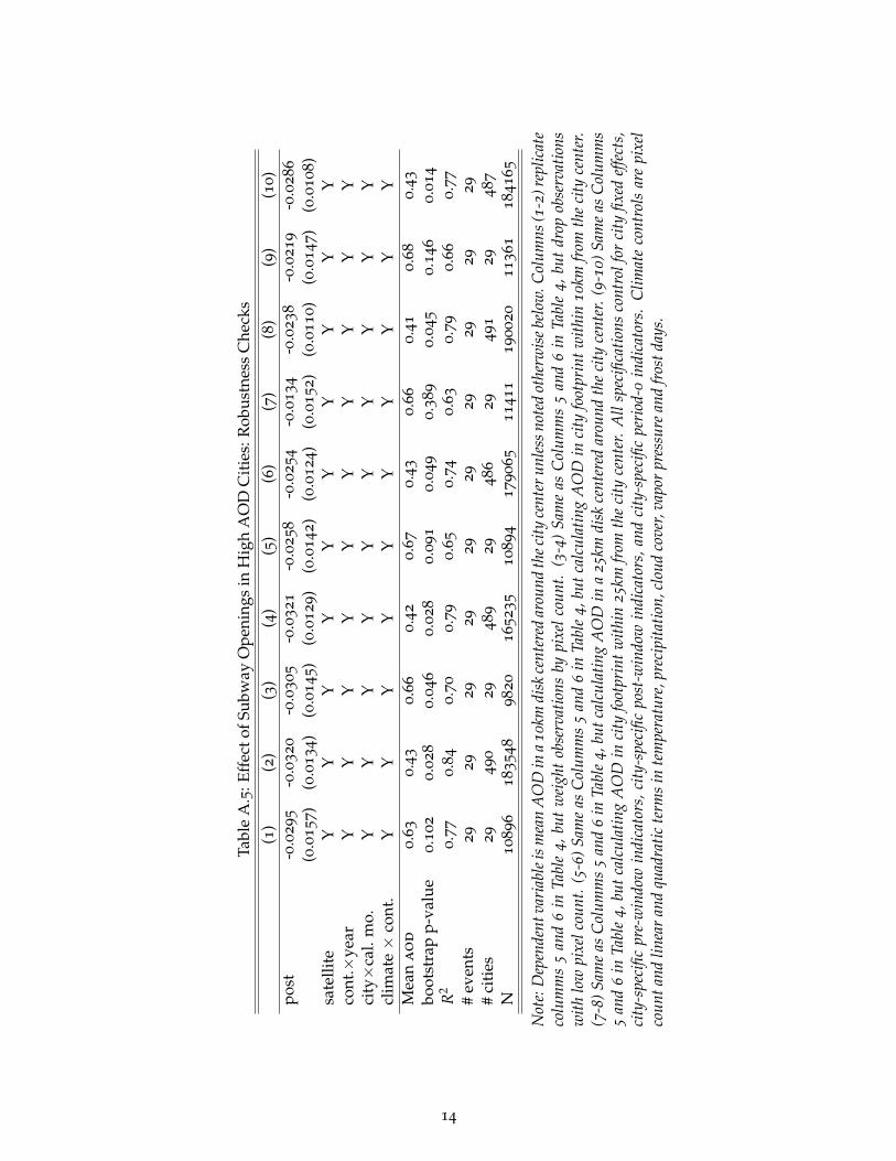
As described in the main text, we obtain RR functions for five diseases: ischemic heart dis-ease, cerebrovascular disease (stroke), chronic obstructive pulmonary disease, lung cancer, andlower respiratory infection. For deaths attributable to stroke and ischemic heart disease, theintegrated risk functions are age-specific. To construct population attributable fractions (PAF)for every disease and, when applicable, every age-group, we first predict pre and post-subwaypm2.5 concentrations using the regression specification in Column 8 of Table A.2. Specifically,we obtain predicted pm2.5 values from the annual city average of AOD (and all other covariates)during the 12 months preceding the subway opening. The post-subway pm2.5 concentrations areobtained by subtracting 0.028× 60.57 = 1.696 µg/m3 to the pre-subway concentration, where 0.028

is the subway AOD effect from Table 4 in the paper, and 60.57 is the AOD coefficient in Column 8

of Table A.2.Let c0 and c1 respectively denote the pre and post-subway pm2.5 concentrations in a given city.

For the purpose of our burden of disease calculations, the relevant risk ratio is RRd(c1,c0) =P(Dd | c1)/P(Dd | c0). Using the RRd(c,c̄) functions in Burnett et al. (2014), we obtain this numberby computing RRd(c1,c0) = RRd(c1,c̄)/RRd(c0,c̄). Here, RRd(c1,c0) expresses how much less likely

Comparing with Table A.2, we see that these coefficient estimates are quite different. The difference reflects primarilyour use of the level of pm2.5 , rather than its logarithm, as the dependent variable. We also use the level of AOD ratherthan its logarithm as the explanatory variable. Since AOD is typically around 0.5, this turns out not to be important.Finally, our sample describes a different and more urban sample of locations, relies on annual rather than daily data, andmeasures AOD using just MODIS data rather than an average of MODIS and a measure imputed using a climate modeland ground based emissions release information. We prefer the formulation in Table A.2 to that in Brauer et al. (2015) forthree reasons. First, AOD is already a logarithm (see footnote 4 in the paper), so the Brauer et al. specification uses thelogarithm of a logarithm as its main explanatory variable. Second, mortality and morbidity estimates are typically basedon levels of pollutants, not on percentage changes, so the dependent variable in our regressions is more immediatelyuseful for evaluating the health implications of changes in AOD. Finally, we control for weather conditions, whichappears to be important. In any case, the R2 in both studies is of similar magnitude.

10

it is that individuals die of disease d when exposed to concentration c1, relative to concentration c0.Assuming that 100% of the city population is exposed to c0 and then c1, the population attributablefraction is then just PAFd = 1−RRd(c1,c0) = 1− P(Dd | c1)/P(Dd | c0). Interpreting P(Dd | c) as thefraction of the total population that died of disease d when exposed to pm2.5 concentration c, wefind that PAFd represents the fraction of total deaths from d that occurred because of incrementalpollution c0 − c1.

Finally, for each high AOD city i, we calculate the number of death attributable to disease din age-group a (denoted Mida below). We use disease-specific country-level death rates from theWorld Health Organisation (WHO, 2016c) and apply them to city populations. Mortality data fromthe WHO is only available in 2000, 2005, 2010, and 2015. We use the year closest to a city’s subwayopening year. The total number of avoided death in city i is given by ∑d ∑a PAFida ·Mida.

11

E Supplemental Tables

Table A.3: Average Effect of Subway Openings: Robustness Checks(1) (2) (3) (4) (5) (6)

post -0.0094 -0.0035 -0.0093 -0.0080 -0.0050 -0.0082(0.0090) (0.0085) (0.0090) (0.0088) (0.0088) (0.0086)

satellite Y Y Y Y Y Ycont.×year Y Y Y Y Y Ycity×cal. mo. Y Y Y Y Y Yclimate × cont. Y Y Y Y Y YMean AOD 0.46 0.41 0.45 0.46 0.45 0.47R2 0.80 0.87 0.84 0.79 0.80 0.80# events 58 58 58 58 58 58# cities 58 58 58 58 58 58N 21806 21806 19635 21702 22605 22497

Note: Dependent variable is mean AOD in a 10km disk with centroid in the city centerunless noted otherwise below. (1) Replicates Column 5 from Table 2 in the paper (forreference). (2) Same as (1) but weight observations by pixel count. (3) Same as (1)but drop observations with low pixel count. (4) Same as (1) but calculating AOD incity footprint within 10km from the city center. (5) Same as (1) but calculating AODin a 25km disk centered around the city center. (6) Same as (1) but calculating AODin city footprint within 25km from the city center. All specifications control for cityfixed effects, city-specific pre-window indicators, city-specific post-window indicators,and city-specific period-0 indicators. Climate controls are pixel count and linear andquadratic terms in temperature, precipitation, cloud cover, vapor pressure and frostdays. Standard errors clustered at the city level in parentheses.

12

Table A.4: Average Effect of Subway Openings: Different Window of Analysis(1) (2) (3) (4) (5)

post -0.0094 -0.0027 -0.0040 -0.0008 -0.0057(0.0090) (0.0108) (0.0096) (0.0084) (0.0088)

satellite Y Y Y Y Ycont.×year Y Y Y Y Ycity×cal. mo. Y Y Y Y Yclimate × cont. Y Y Y Y YMean AOD 0.46 0.46 0.46 0.44 0.45R2 0.80 0.80 0.81 0.81 0.81# events 58 64 60 55 44# cities 58 64 60 55 44N 21806 24028 22580 20684 16422

Note: Dependent variable is mean AOD in a 10km disk centered aroundthe city center. (1) Column 5, Table 2 in the paper (for reference). (2) Sameas (1) but treatment and control window are 6 months. (3) Same as (1)but treatment and control window are 12 months. (4) Same as (1) buttreatment and control window are 24 months. (5) Same as (1) but treat-ment and control window are 36 months. All specifications control for cityfixed effects, city-specific pre-window indicators, city-specific post-windowindicators, and city-specific period-0 indicators. Climate controls are pixelcount and linear and quadratic terms in temperature, precipitation, cloudcover, vapor pressure and frost days. Standard errors clustered at the citylevel in parentheses.

13

Tabl

eA

.5:E

ffec

tofS

ubw

ayO

peni

ngs

inH

igh

AO

DC

itie

s:R

obus

tnes

sC

heck

s(1

)(2

)(3

)(4

)(5

)(6

)(7

)(8

)(9

)(1

0)

post

-0.0

295

-0.0

320

-0.0

305

-0.0

321

-0.0

258

-0.0

254

-0.0

134

-0.0

238

-0.0

219

-0.0

286

(0.0

157)

(0.0

134)

(0.0

145

)(0

.0129)

(0.0

142)

(0.0

124)

(0.0

152)

(0.0

110)

(0.0

147)

(0.0

108)

sate

llite

YY

YY

YY

YY

YY

cont

.×ye

arY

YY

YY

YY

YY

Yci

ty×

cal.

mo.

YY

YY

YY

YY

YY

clim

ate×

cont

.Y

YY

YY

YY

YY

YM

ean

ao

d0.6

30.4

30.6

60.4

20.6

70.4

30.6

60.4

10.6

80.4

3

boot

stra

pp-

valu

e0.1

02

0.0

28

0.0

46

0.0

28

0.0

91

0.0

49

0.3

89

0.0

45

0.1

46

0.0

14

R2

0.7

70.8

40.7

00.7

90.6

50.7

40.6

30.7

90.6

60.7

7

#ev

ents

29

29

29

29

29

29

29

29

29

29

#ci

ties

29

490

29

489

29

486

29

491

29

487

N10896

183548

9820

165235

10894

179065

11411

190020

11361

184165

Not

e:D

epen

dent

vari

able

ism

ean

AO

Din

a10

kmdi

skce

nter

edar

ound

thec

ityce

nter

unle

ssno

ted

othe

rwis

ebel

ow.C

olum

ns(1

-2)r

eplic

ate

colu

mm

s5

and

6in

Tabl

e4,

but

wei

ght

obse

rvat

ions

bypi

xelc

ount

.(3

-4)

Sam

eas

Col

umm

s5

and

6in

Tabl

e4,

but

drop

obse

rvat

ions

with

low

pixe

lcou

nt.

(5-6

)Sam

eas

Col

umm

s5

and

6in

Tabl

e4,

butc

alcu

latin

gA

OD

inci

tyfo

otpr

intw

ithin

10km

from

the

city

cent

er.

(7-8

)Sam

eas

Col

umm

s5

and

6in

Tabl

e4,

butc

alcu

latin

gA

OD

ina

25km

disk

cent

ered

arou

ndth

eci

tyce

nter

.(9-

10)S

ame

asC

olum

ms

5an

d6

inTa

ble

4,bu

tcal

cula

ting

AO

Din

city

foot

prin

twith

in25

kmfr

omth

eci

tyce

nter

.A

llsp

ecifi

catio

nsco

ntro

lfor

city

fixed

effe

cts,

city

-spe

cific

pre-

win

dow

indi

cato

rs,c

ity-s

peci

ficpo

st-w

indo

win

dica

tors

,and

city

-spe

cific

peri

od-0

indi

cato

rs.

Clim

ate

cont

rols

are

pixe

lco

unta

ndlin

ear

and

quad

ratic

term

sin

tem

pera

ture

,pre

cipi

tatio

n,cl

oud

cove

r,va

por

pres

sure

and

fros

tday

s.

14

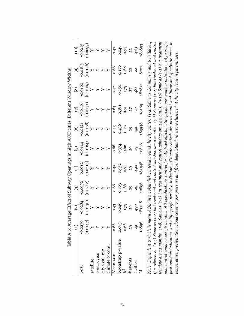
Tabl

eA

.6:A

vera

geEf

fect

ofSu

bway

Ope

ning

sin

high

AO

Dci

ties

:Diff

eren

tWin

dow

Wid

ths

(1)

(2)

(3)

(4)

(5)

(6)

(7)

(8)

(9)

(10)

post

-0.0

270

-0.0

284

-0.0

032

0.0

012

-0.0

144

-0.0

121

-0.0

116

-0.0

160

-0.0

185

-0.0

215

(0.0

147)

(0.0

130)

(0.0

212

)(0

.0215)

(0.0

164)

(0.0

158)

(0.0

131)

(0.0

109)

(0.0

136)

(0.0

099)

sate

llite

YY

YY

YY

YY

YY

cont

.×ye

arY

YY

YY

YY

YY

Yci

ty×

cal.

mo.

YY

YY

YY

YY

YY

clim

ate×

cont

.Y

YY

YY

YY

YY

YM

ean

ao

d0.6

60.4

30.6

60.4

30.6

60.4

30.6

40.4

20.6

60.4

2

boot

stra

pp-

valu

e0.0

83

0.0

49

0.8

63

0.9

52

0.3

74

0.4

36

0.3

81

0.1

50

0.1

70

0.0

46

R2

0.6

60.7

50.6

60.7

50.6

60.7

50.7

00.7

50.6

80.7

5

#ev

ents

29

29

29

29

29

29

27

27

22

22

#ci

ties

29

490

29

490

29

490

27

488

22

483

N10896

183548

10896

183548

10896

183548

10169

182821

8201

180853

Not

e:D

epen

dent

vari

able

ism

ean

AO

Din

a10

kmdi

skce

nter

edar

ound

the

city

cent

er.

(1-2

)Sam

eas

Col

umm

s5

and

6in

Tabl

e4

(for

refe

renc

e).

(3-4

)Sa

me

as(1

-2)

but

trea

tmen

tan

dco

ntro

lwin

dow

are

6m

onth

s.(5

-6)

Sam

eas

(1-2

)bu

ttr

eatm

ent

and

cont

rol

win

dow

are

12m

onth

s.(7

-8)

Sam

eas

(1-2

)bu

ttr

eatm

ent

and

cont

rolw

indo

war

e24

mon

ths.

(9-1

0)Sa

me

as(1

-2)

but

trea

tmen

tan

dco

ntro

lwin

dow

are

36m

onth

s.A

llsp

ecifi

catio

nsco

ntro

lfor

city

fixed

effe

cts,

city

-spe

cific

pre-

win

dow

indi

cato

rs,c

ity-s

peci

ficpo

st-w

indo

win

dica

tors

,an

dci

ty-s

peci

ficpe

riod

-0in

dica

tors

.C

limat

eco

ntro

lsar

epi

xel

coun

tan

dlin

ear

and

quad

ratic

term

sin

tem

pera

ture

,pre

cipi

tatio

n,cl

oud

cove

r,va

por

pres

sure

and

fros

tday

s.St

anda

rder

rors

clus

tere

dat

the

city

leve

lin

pare

nthe

ses.

15

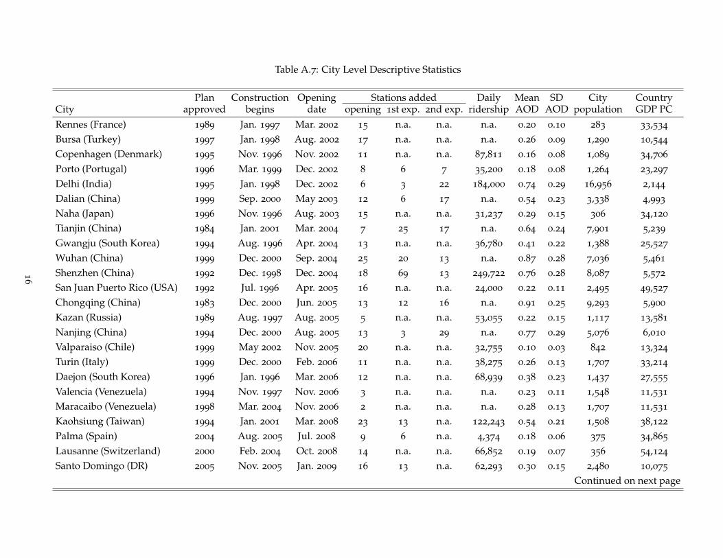
Table A.7: City Level Descriptive Statistics

Plan Construction Opening Stations added Daily Mean SD City CountryCity approved begins date opening 1st exp. 2nd exp. ridership AOD AOD population GDP PCRennes (France) 1989 Jan. 1997 Mar. 2002 15 n.a. n.a. n.a. 0.20 0.10 283 33,534

Bursa (Turkey) 1997 Jan. 1998 Aug. 2002 17 n.a. n.a. n.a. 0.26 0.09 1,290 10,544

Copenhagen (Denmark) 1995 Nov. 1996 Nov. 2002 11 n.a. n.a. 87,811 0.16 0.08 1,089 34,706

Porto (Portugal) 1996 Mar. 1999 Dec. 2002 8 6 7 35,200 0.18 0.08 1,264 23,297

Delhi (India) 1995 Jan. 1998 Dec. 2002 6 3 22 184,000 0.74 0.29 16,956 2,144

Dalian (China) 1999 Sep. 2000 May 2003 12 6 17 n.a. 0.54 0.23 3,338 4,993

Naha (Japan) 1996 Nov. 1996 Aug. 2003 15 n.a. n.a. 31,237 0.29 0.15 306 34,120

Tianjin (China) 1984 Jan. 2001 Mar. 2004 7 25 17 n.a. 0.64 0.24 7,901 5,239

Gwangju (South Korea) 1994 Aug. 1996 Apr. 2004 13 n.a. n.a. 36,780 0.41 0.22 1,388 25,527

Wuhan (China) 1999 Dec. 2000 Sep. 2004 25 20 13 n.a. 0.87 0.28 7,036 5,461

Shenzhen (China) 1992 Dec. 1998 Dec. 2004 18 69 13 249,722 0.76 0.28 8,087 5,572

San Juan Puerto Rico (USA) 1992 Jul. 1996 Apr. 2005 16 n.a. n.a. 24,000 0.22 0.11 2,495 49,527

Chongqing (China) 1983 Dec. 2000 Jun. 2005 13 12 16 n.a. 0.91 0.25 9,293 5,900

Kazan (Russia) 1989 Aug. 1997 Aug. 2005 5 n.a. n.a. 53,055 0.22 0.15 1,117 13,581

Nanjing (China) 1994 Dec. 2000 Aug. 2005 13 3 29 n.a. 0.77 0.29 5,076 6,010

Valparaiso (Chile) 1999 May 2002 Nov. 2005 20 n.a. n.a. 32,755 0.10 0.03 842 13,324

Turin (Italy) 1999 Dec. 2000 Feb. 2006 11 n.a. n.a. 38,275 0.26 0.13 1,707 33,214

Daejon (South Korea) 1996 Jan. 1996 Mar. 2006 12 n.a. n.a. 68,939 0.38 0.23 1,437 27,555

Valencia (Venezuela) 1994 Nov. 1997 Nov. 2006 3 n.a. n.a. n.a. 0.23 0.11 1,548 11,531

Maracaibo (Venezuela) 1998 Mar. 2004 Nov. 2006 2 n.a. n.a. n.a. 0.28 0.13 1,707 11,531

Kaohsiung (Taiwan) 1994 Jan. 2001 Mar. 2008 23 13 n.a. 122,243 0.54 0.21 1,508 38,122

Palma (Spain) 2004 Aug. 2005 Jul. 2008 9 6 n.a. 4,374 0.18 0.06 375 34,865

Lausanne (Switzerland) 2000 Feb. 2004 Oct. 2008 14 n.a. n.a. 66,852 0.19 0.07 356 54,124

Santo Domingo (DR) 2005 Nov. 2005 Jan. 2009 16 13 n.a. 62,293 0.30 0.15 2,480 10,075

Continued on next page

16

Table A.7 – continued from previous pagePlan Construction Opening Stations added Daily Mean SD City Country

City approved begins date opening 1st exp. 2nd exp. ridership AOD AOD population GDP PCAdana (Turkey) 1988 Sep. 1996 Mar. 2009 8 n.a. n.a. n.a. 0.33 0.12 1,453 16,317

Seville (Spain) 1999 Aug. 2005 Apr. 2009 17 n.a. n.a. 43,461 0.20 0.08 694 34,496

Seattle (USA) 1996 Nov. 2003 Jul. 2009 8 n.a. n.a. 15,437 0.17 0.08 3,017 49,706

Dubai (UAE) 2005 Mar. 2006 Sep. 2009 10 16 n.a. 169,816 0.51 0.24 1,699 65,788

Chengdu (China) 2000 Dec. 2005 Sep. 2010 16 20 5 n.a. 0.90 0.32 7,481 9,131

Shenyang (China) 1999 Nov. 2005 Sep. 2010 22 19 n.a. 434,428 0.48 0.26 5,819 9,131

Xian, Shaanxi (China) 1994 Sep. 2006 Sep. 2011 17 26 n.a. 295,220 0.73 0.25 5,684 10,043

Bangalore (India) 2003 Apr. 2007 Oct. 2011 7 10 n.a. 18,436 0.47 0.12 8,579 4,461

Mashhad (Iran) 1994 Dec. 1999 Oct. 2011 21 6 n.a. 83,345 0.22 0.10 2,717 18,195

Algiers (Algeria) 1988 Mar. 1993 Nov. 2011 10 n.a. n.a. n.a. 0.33 0.17 2,461 13,342

Almaty (Kazakhstan) 1980 Sep. 1988 Dec. 2011 7 n.a. n.a. 18,228 0.25 0.06 1,470 22,022

Lima (Peru) 1986 Oct. 1986 Apr. 2012 16 n.a. n.a. 120,575 0.71 0.19 9,150 10,496

Suzhou, Jiangsu (China) 2002 Dec. 2007 Apr. 2012 24 20 38 196,778 0.81 0.25 4,326 10,365

Kunming (China) 2009 May 2010 Jun. 2012 2 12 18 n.a. 0.31 0.24 3,602 10,423

Hangzhou (China) 2005 Mar. 2007 Nov. 2012 31 13 10 390,595 0.79 0.22 6,112 10,568

Brescia (Italy) 2000 Jan. 2004 Mar. 2013 17 n.a. n.a. 42,943 0.27 0.14 452 36,113

Harbin (China) 2005 Sep. 2009 Sep. 2013 17 n.a. n.a. 182,333 0.30 0.18 5,457 11,041

Zhengzhou (China) 2008 Jun. 2009 Dec. 2013 20 15 20 244,722 0.83 0.34 4,074 11,189

Changsha (China) 2008 Sep. 2009 Apr. 2014 18 n.a. n.a. 233,528 0.83 0.25 3,799 11,374

Panama City (Panama) 2009 Feb. 2011 Apr. 2014 12 n.a. n.a. 223,661 0.33 0.14 1,615 18,887

Ningbo (China) 2003 Jun. 2009 May 2014 20 21 n.a. 104,889 0.81 0.22 3,187 11,420

Mumbai (India) 2004 Feb. 2008 Jun. 2014 12 n.a. n.a. 260,000 0.59 0.35 18,992 5,095

Salvador da Bahia (Brazil) 1999 Apr. 2000 Jun. 2014 5 2 n.a. 42,782 0.20 0.07 3,517 15,231

Wuxi (China) 2006 Nov. 2009 Jul. 2014 24 18 n.a. 229,642 0.84 0.24 2,915 11,513

Shiraz (Iran) 1993 Jun. 2006 Oct. 2014 5 n.a. n.a. n.a. 0.27 0.09 1,513 15,816

Continued on next page

17

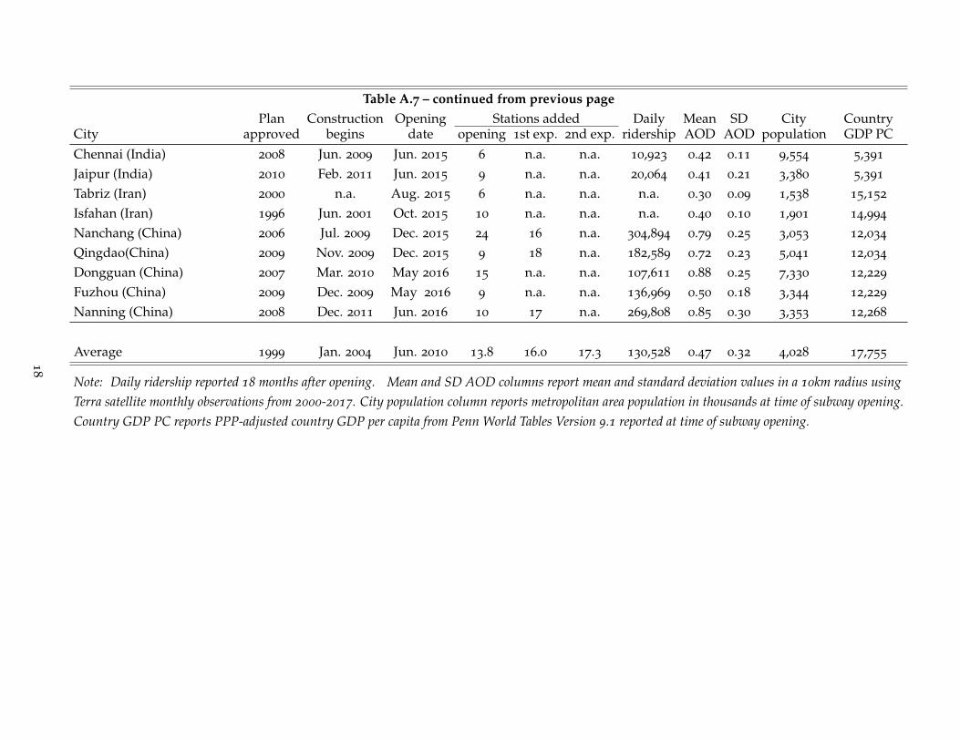
Table A.7 – continued from previous pagePlan Construction Opening Stations added Daily Mean SD City Country

City approved begins date opening 1st exp. 2nd exp. ridership AOD AOD population GDP PCChennai (India) 2008 Jun. 2009 Jun. 2015 6 n.a. n.a. 10,923 0.42 0.11 9,554 5,391

Jaipur (India) 2010 Feb. 2011 Jun. 2015 9 n.a. n.a. 20,064 0.41 0.21 3,380 5,391

Tabriz (Iran) 2000 n.a. Aug. 2015 6 n.a. n.a. n.a. 0.30 0.09 1,538 15,152

Isfahan (Iran) 1996 Jun. 2001 Oct. 2015 10 n.a. n.a. n.a. 0.40 0.10 1,901 14,994

Nanchang (China) 2006 Jul. 2009 Dec. 2015 24 16 n.a. 304,894 0.79 0.25 3,053 12,034

Qingdao(China) 2009 Nov. 2009 Dec. 2015 9 18 n.a. 182,589 0.72 0.23 5,041 12,034

Dongguan (China) 2007 Mar. 2010 May 2016 15 n.a. n.a. 107,611 0.88 0.25 7,330 12,229

Fuzhou (China) 2009 Dec. 2009 May 2016 9 n.a. n.a. 136,969 0.50 0.18 3,344 12,229

Nanning (China) 2008 Dec. 2011 Jun. 2016 10 17 n.a. 269,808 0.85 0.30 3,353 12,268

Average 1999 Jan. 2004 Jun. 2010 13.8 16.0 17.3 130,528 0.47 0.32 4,028 17,755

Note: Daily ridership reported 18 months after opening. Mean and SD AOD columns report mean and standard deviation values in a 10km radius usingTerra satellite monthly observations from 2000-2017. City population column reports metropolitan area population in thousands at time of subway opening.Country GDP PC reports PPP-adjusted country GDP per capita from Penn World Tables Version 9.1 reported at time of subway opening.

18

F Supplemental Figures

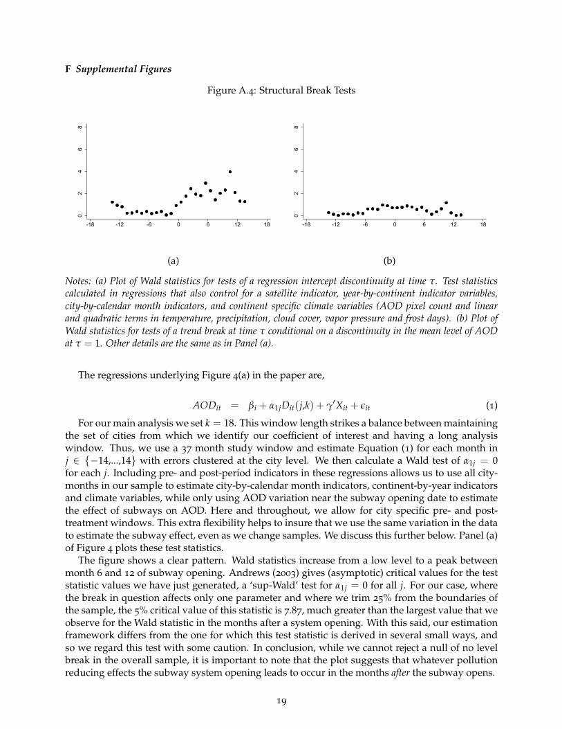
Figure A.4: Structural Break Tests0

24

68

-18 -12 -6 0 6 12 18

02

46

8

-18 -12 -6 0 6 12 18

(a) (b)

Notes: (a) Plot of Wald statistics for tests of a regression intercept discontinuity at time τ. Test statisticscalculated in regressions that also control for a satellite indicator, year-by-continent indicator variables,city-by-calendar month indicators, and continent specific climate variables (AOD pixel count and linearand quadratic terms in temperature, precipitation, cloud cover, vapor pressure and frost days). (b) Plot ofWald statistics for tests of a trend break at time τ conditional on a discontinuity in the mean level of AODat τ = 1. Other details are the same as in Panel (a).

The regressions underlying Figure 4(a) in the paper are,

AODit = βi + α1jDit(j,k) + γ′Xit + εit (1)

For our main analysis we set k = 18. This window length strikes a balance between maintainingthe set of cities from which we identify our coefficient of interest and having a long analysiswindow. Thus, we use a 37 month study window and estimate Equation (1) for each month inj ∈ {−14,...,14} with errors clustered at the city level. We then calculate a Wald test of α1j = 0for each j. Including pre- and post-period indicators in these regressions allows us to use all city-months in our sample to estimate city-by-calendar month indicators, continent-by-year indicatorsand climate variables, while only using AOD variation near the subway opening date to estimatethe effect of subways on AOD. Here and throughout, we allow for city specific pre- and post-treatment windows. This extra flexibility helps to insure that we use the same variation in the datato estimate the subway effect, even as we change samples. We discuss this further below. Panel (a)of Figure 4 plots these test statistics.

The figure shows a clear pattern. Wald statistics increase from a low level to a peak betweenmonth 6 and 12 of subway opening. Andrews (2003) gives (asymptotic) critical values for the teststatistic values we have just generated, a ‘sup-Wald’ test for α1j = 0 for all j. For our case, wherethe break in question affects only one parameter and where we trim 25% from the boundaries ofthe sample, the 5% critical value of this statistic is 7.87, much greater than the largest value that weobserve for the Wald statistic in the months after a system opening. With this said, our estimationframework differs from the one for which this test statistic is derived in several small ways, andso we regard this test with some caution. In conclusion, while we cannot reject a null of no levelbreak in the overall sample, it is important to note that the plot suggests that whatever pollutionreducing effects the subway system opening leads to occur in the months after the subway opens.

19

In Figure 4(b) in the paper we check for a change in the trend of AOD associated with subwayopenings. We proceed much as in our test for a break, but instead look for a change in trendaround the time of a subway opening conditional on a level break at τ = 1. Formally, this meansestimating the following set of regressions,

AODit = βi + α1τit + α2jτitDit(j,k) + α3Dit(1,k) + γ′Xit + εit (2)

As before, we estimate the regression (2) for each month in j ∈ {−14,...,14}with errors clusteredat the city level and calculate the Wald test for α2 = 0 for each regression.5 Panel (b) of Figure 4

in the paper plots these Wald statistic values as j varies.6 Thus, conditional on a step at τ = 1,subways openings do not seem to cause a change in the trend of AOD in a city.

5An alternative would be to simultaneously search for locations of the break and trend break. Hansen (2000) arguesthat sequential searching, as we do, arrives at the same result.

6All values are well below the 10% critical value of 6.35 given in Andrews (2003). Again, our framework differs fromthe framework under which this test statistic is derived so this test should be regarded with caution.

20

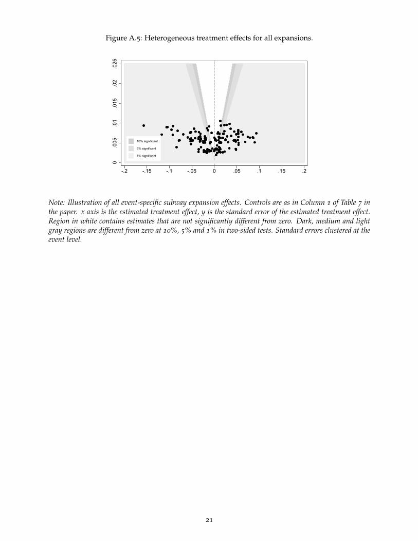
Figure A.5: Heterogeneous treatment effects for all expansions.

0.0

05.0

1.0

15.0

2.0

25

-.2 -.15 -.1 -.05 0 .05 .1 .15 .2

10% significant

5% significant

1% significant

Note: Illustration of all event-specific subway expansion effects. Controls are as in Column 1 of Table 7 inthe paper. x axis is the estimated treatment effect, y is the standard error of the estimated treatment effect.Region in white contains estimates that are not significantly different from zero. Dark, medium and lightgray regions are different from zero at 10%, 5% and 1% in two-sided tests. Standard errors clustered at theevent level.

21

References

Andrews, Donald W.K. 2003. Tests for parameter instability and structural change with unknownchange point: A corrigendum. Econometrica : 395–397.

Brauer, Michael, Greg Freedman, Joseph Frostad, Aaron Van Donkelaar, Randall V. Martin, FrankDentener, Rita van Dingenen, Kara Estep, Heresh Amini, and Joshua S. Apte. 2015. Ambientair pollution exposure estimation for the global burden of disease 2013. Environmental Science &Technology 50(1): 79–88.

Burnett, Richard T et al. 2014. An integrated risk function for estimating the global burden of dis-ease attributable to ambient fine particulate matter exposure. Environmental Health Perspectives122(4): 397.

Gonzalez-Navarro, Marco and Matthew A Turner. 2018. Subways and urban growth: Evidencefrom earth. Journal of Urban Economics 108: 85–106.

Gupta, Pawan, Sundar A. Christopher, Jun Wang, Robert Gehrig, Yc Lee, and Naresh Kumar.2006. Satellite remote sensing of particulate matter and air quality assessment over global cities.Atmospheric Environment 40: 5880–5892.

Hansen, Bruce E. 2000. Testing for structural change in conditional models. Journal of Econometrics97(1): 93–115.

Kumar, Naresh, Allen Chu, and Andrew Foster. 2007. An empirical relationship between pm2.5and aerosol optical depth in Delhi metropolitan. Atmospheric Environment 41: 4492–4503.

Kumar, Naresh, Allen D. Chu, Andrew D. Foster, Thomas Peters, and Robert Willis. 2011. Satelliteremote sensing for developing time and space resolved estimates of ambient particulate inCleveland, OH. Aerosol Science and Technology 45: 1090–1108.

World Health Organization. 2006. WHO air quality guidelines. Geneva: World Health Organiza-tion.

World Health Organization. 2016a. Global urban ambient air pollution database.http://www.who.int/phe/health_topics/outdoorair/databases/cities/en/. Accessed:2017-04-10.

World Health Organization. 2016c. Global health estimates 2015: Deaths by cause, age, sex, bycountry and by region, 2000-2015.

22