online appendix for digitization and flexibility: evidence

Online Appendix

for

Digitization and Flexibility:

Evidence from the South Korean Movie Market

Joonhyuk Yang Eric T. Anderson Brett R. Gordon

Kellogg School of Management

Northwestern University

(A) A model of theaters’ scheduling decisions

(B) A natural experiment for supply concentration

(C) Additional figures and tables

1

A A model of theaters’ scheduling decisions

A.1 The model

A profit-maximizing theater decides the optimal allocation of screens to J movies by solving the fol-

lowing optimization problem:

maxa∈A

π(a) =∑

j∈J

R j (a j )−C (a j )

subject to a j ∈Q≥0, ∀ j (non-negativity constraint)∑

j∈J

a j ≤ K (capacity constraint)

(A.1)

The decision variable is a= (a1, ..., a J )where each element represents the number of screens the theater

allots to each movie. Both revenue, R j , and cost, C j , are a function of screen allocation. Note that a j

can take a value of either zero or a positive rational number. For instance, a j = 0 indicates that the

theater does not show movie j and a j = 0.5 indicates that j is shown in a screen but only for a half-day.

K is the capacity of the theater (i.e., total number of screens).1

Revenue function We specify the theater’s revenue function as follows:

R j (a j ) =�

pj · (1−θ j ) +κ�

·q j (a j ), (A.2)

where pj is ticket price, θ j is the fraction of revenue the theater pays to distributors, κ is average con-

cession profit per moviegoer. q j (a j ) is ticket sales, which is assumed to increase in a j at a diminishing

return (∂ q j /∂ a j ≥ 0 and ∂ 2q j /∂ a 2j ≤ 0). We assume that the ticket price and revenue sharing ra-

tio are invariant across movies.2 Then, the revenue function simplifies to R j (a j ) = r̃ · q j (a j ), where

r̃ = p · (1−θ ) +κ is common across movies.

We take into account the heterogeneity in movies’ commercial appeal to consumers. To capture

this environment, without loss of generality, we assume that q1(a ) > q2(a ) > q3(a ) > ... > qJ (a ) for any

value of a . In particular, we consider that j = 1 represents the top movie, where q1(·) is sufficiently

greater than the demand for any other movies available in the market.

Cost function We consider two types of costs associated with showing movie j in a j screens: the

cost of acquiring a copy (or copies) of a movie and the cost of scheduling movies within a screen. The

scheduling cost represents the marginal and/or fixed cost of labor required to change the movie playing

1For the sake of parsimonious representation, we abstract away from other important dimensions of scheduling prob-lems, which include theater size, competition, dynamic decisions, and ex ante demand uncertainty.

2We consider a flat ratio to simplify the model and, more importantly, it is the case in our empirical context.

2

on a screen. To capture both types, we specify the cost function as follows:

C (a j ) = c1

�

a j

�

+c2

2I��

a j

�

−a j > 0

, (A.3)

where�

a j

�

is the ceiling, or the smallest integer that is greater than or equal to a j (similarly, we define�

a j

�

as the floor, or the greatest integer that is smaller than or equal to a j ). c1 and c2 are nonnega-

tive cost parameters. The first term captures the acquisition cost of movies.3 For instance, if the the-

ater wants to show movie j in three screens simultaneously, it has to pay a cost of 3c1.4 The second

term captures a scheduling cost that occurs when theaters switch between movies across slots within

a screen. We assume that the theater pays a scheduling cost (c2/2) when it allots a fraction of a screen

to a movie. So, a theater has to pay c2 if a screen shows two different movies, whereas this cost is zero

if a single title is shown on the screen. Note that�

a j

�

−a j > 0 is true only if a j is a non-integer value.

Figure A.1 provides a graphical illustration of the cost function. Suppose that a theater considers

three options for the number of screen it allots to a movie:�

a j

�

, a j , and�

a j

�

. Showing a movie in�

a j

�

screens costs c1

�

a j

�

as point A in the figure indicates. Similarly, showing a movie in�

a j

�

screens

costs c1

�

a j

�

(point B in the figure). Lastly, if the theater shows a movie in a j screens, which can be

a non-integer rational number, it has to pay c1

�

a j

�

for the cost of acquisition and c2/2 for the cost of

scheduling (point C ).

Figure A.1: An illustration of cost function

a j

C (a j )

y = c1a j

c1

�

a j

�

c1

�

a j

�

c1

�

a j

�

+ c2/2

A

B

C

�

a j

� a j�

a j

�

The key intuition embedded in our cost function is that the cost of flexibility, such as when a theater

allocates more than one movie to a single screen, exists in scheduling problems. Depending on the

relative magnitude of parameters, the cost may induce theaters to find suboptimal solutions in terms

3The parameter captures both the price actual dollar amount a theater has to pay4To capture a form of quantity discount, we can change this term to be nonlinear (e.g., quadratic). This does not change

the model’s predictions.

3

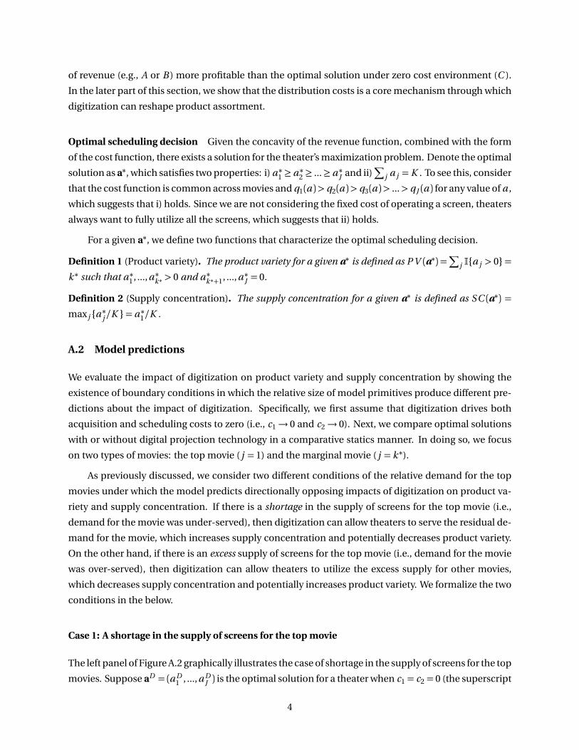
of revenue (e.g., A or B ) more profitable than the optimal solution under zero cost environment (C ).

In the later part of this section, we show that the distribution costs is a core mechanism through which

digitization can reshape product assortment.

Optimal scheduling decision Given the concavity of the revenue function, combined with the form

of the cost function, there exists a solution for the theater’s maximization problem. Denote the optimal

solution as a∗, which satisfies two properties: i) a ∗1 ≥ a ∗2 ≥ ...≥ a ∗J and ii)∑

j a j = K . To see this, consider

that the cost function is common across movies and q1(a )> q2(a )> q3(a )> ...> qJ (a ) for any value of a ,

which suggests that i) holds. Since we are not considering the fixed cost of operating a screen, theaters

always want to fully utilize all the screens, which suggests that ii) holds.

For a given a∗, we define two functions that characterize the optimal scheduling decision.

Definition 1 (Product variety). The product variety for a given a∗ is defined as P V (a∗) =∑

j I{a j > 0}=k ∗ such that a ∗1 , ..., a ∗k ∗ > 0 and a ∗k ∗+1, ..., a ∗J = 0.

Definition 2 (Supply concentration). The supply concentration for a given a∗ is defined as SC (a∗) =

max j {a ∗j /K }= a ∗1/K .

A.2 Model predictions

We evaluate the impact of digitization on product variety and supply concentration by showing the

existence of boundary conditions in which the relative size of model primitives produce different pre-

dictions about the impact of digitization. Specifically, we first assume that digitization drives both

acquisition and scheduling costs to zero (i.e., c1→ 0 and c2→ 0). Next, we compare optimal solutions

with or without digital projection technology in a comparative statics manner. In doing so, we focus

on two types of movies: the top movie ( j = 1) and the marginal movie ( j = k ∗).

As previously discussed, we consider two different conditions of the relative demand for the top

movies under which the model predicts directionally opposing impacts of digitization on product va-

riety and supply concentration. If there is a shortage in the supply of screens for the top movie (i.e.,

demand for the movie was under-served), then digitization can allow theaters to serve the residual de-

mand for the movie, which increases supply concentration and potentially decreases product variety.

On the other hand, if there is an excess supply of screens for the top movie (i.e., demand for the movie

was over-served), then digitization can allow theaters to utilize the excess supply for other movies,

which decreases supply concentration and potentially increases product variety. We formalize the two

conditions in the below.

Case 1: A shortage in the supply of screens for the top movie

The left panel of Figure A.2 graphically illustrates the case of shortage in the supply of screens for the top

movies. Suppose aD = (a D1 , ..., a D

J ) is the optimal solution for a theater when c1 = c2 = 0 (the superscript

4

Figure A.2: The relative demand and the impact of digitization

(a) A shortage in supply case (high q )

a j

C (a j )

A

C

�

a D1

�

a D1

∆s

CA

CC

(b) An excess supply case (low q )

a j

C (a j )

B

C

a D1

�

a D1

�

∆e

CB

CC

D represents digital projection). Consider a situation in which the theater finds a F1 =

�

a D1

�

optimal if

c1 and c2 are strictly greater than zero (the superscript F represents film projection). ∆s = a Dj − a F

j

represents the level of shortage in the supply of screens for the top movies. In this case, digitization

increases supply concentration from SC (aF ) = ba D1 c/K to SC (aD ) = a D

1 /K .

When is this likely the case? To see this, consider the following inequality that can be derived from

the setup:5

c1+ c2︸︷︷︸

Cost of flexibility

> r̃1(q1(aD1 )−q1(a

F1 ))

︸︷︷︸

Gain from residual demand

+ r̃J (qJ (aDJ )−qJ (1))

︸︷︷︸

Loss from marginal movie

, (A.4)

where the LHS represents the cost of flexibility, which incurs when splitting a screen for two movies.

The two terms in the RHS represent the gain from serving the residual demand of the top movie and

the loss from allotting fewer screens to marginal movies. By construction, the first term is greater than

zero, whereas the second term is smaller than zero. The sum of the two terms together constitutes the

efficiency gains of digital projection. The inequality indicates that if the cost of flexibility (LHS) is not

justified by the efficiency gains (RHS), a theater would rather give up on trying to serve the residual

demand of the top movie that can arise from a shortage in the supply of screens (i.e.,∆s ). In this case,

digitization can decrease product variety if additional showings of the top movies crowds out marginal

movies. Hence, the model produce the following predictions:

Prediction 1: If there is a shortage in the supply of screens for the top movie (i.e., if Eq. A.4 holds),

(P1a) digitization increases movie concentration in theaters, and

(P1b) digitization weakly decreases the variety of movies offered by theaters.

5The demand condition can be represented as R1(a F1 )−C (a F

1 )+∑

j>1 R1(a j )−C (a j )>R1(a D1 )−C (a D

1 )+∑

j>1 R1(a j )−C (a j ).Later we show that Equation A.4 can be derived from this inequality.

5

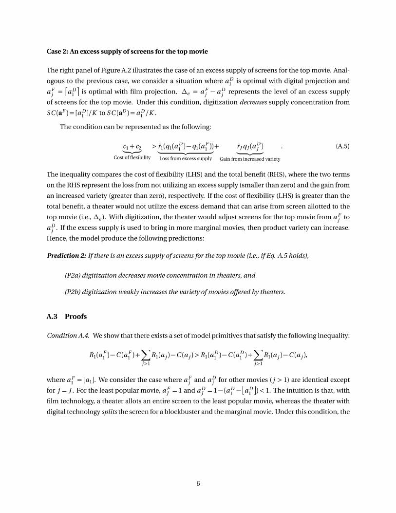
Case 2: An excess supply of screens for the top movie

The right panel of Figure A.2 illustrates the case of an excess supply of screens for the top movie. Anal-

ogous to the previous case, we consider a situation where a D1 is optimal with digital projection and

a Fj =

�

a D1

�

is optimal with film projection. ∆e = a Fj − a D

j represents the level of an excess supply

of screens for the top movie. Under this condition, digitization decreases supply concentration from

SC (aF ) = da D1 e/K to SC (aD ) = a D

1 /K .

The condition can be represented as the following:

c1+ c2︸︷︷︸

Cost of flexibility

> r̃1(q1(aD1 )−q1(a

F1 ))

︸︷︷︸

Loss from excess supply

+ r̃J qJ (aDJ )

︸︷︷︸

Gain from increased variety

. (A.5)

The inequality compares the cost of flexibility (LHS) and the total benefit (RHS), where the two terms

on the RHS represent the loss from not utilizing an excess supply (smaller than zero) and the gain from

an increased variety (greater than zero), respectively. If the cost of flexibility (LHS) is greater than the

total benefit, a theater would not utilize the excess demand that can arise from screen allotted to the

top movie (i.e., ∆e ). With digitization, the theater would adjust screens for the top movie from a Fj to

a Dj . If the excess supply is used to bring in more marginal movies, then product variety can increase.

Hence, the model produce the following predictions:

Prediction 2: If there is an excess supply of screens for the top movie (i.e., if Eq. A.5 holds),

(P2a) digitization decreases movie concentration in theaters, and

(P2b) digitization weakly increases the variety of movies offered by theaters.

A.3 Proofs

Condition A.4. We show that there exists a set of model primitives that satisfy the following inequality:

R1(aF1 )−C (a F

1 ) +∑

j>1

R1(a j )−C (a j )>R1(aD1 )−C (a D

1 ) +∑

j>1

R1(a j )−C (a j ),

where a F1 = ba1c. We consider the case where a F

j and a Dj for other movies ( j > 1) are identical except

for j = J . For the least popular movie, a FJ = 1 and a D

J = 1− (a D1 −

�

a D1

�

) < 1. The intuition is that, with

film technology, a theater allots an entire screen to the least popular movie, whereas the theater with

digital technology splits the screen for a blockbuster and the marginal movie. Under this condition, the

6

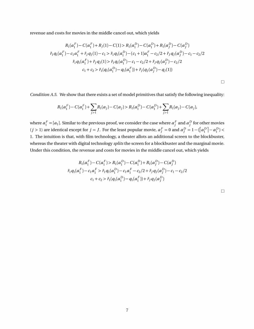
revenue and costs for movies in the middle cancel out, which yields

R1(aF1 )−C (a F

1 ) +R J (1)−C (1)>R1(aD1 )−C (a D

1 ) +R1(aDJ )−C (a D

J )

r̃1q1(aF1 )− c1a F

1 + r̃J qJ (1)− c1 > r̃1q1(aD1 )− (c1+1)a F

1 − c2/2+ r̃J qJ (aDJ )− c1− c2/2

r̃1q1(aF1 ) + r̃J qJ (1)> r̃1q1(a

D1 )− c1− c2/2+ r̃J qJ (a

DJ )− c2/2

c1+ c2 > r̃1(q1(aD1 )−q1(a

F1 ))+ r̃J (qJ (a

DJ )−qJ (1))

Condition A.5. We show that there exists a set of model primitives that satisfy the following inequality:

R1(aF1 )−C (a F

1 ) +∑

j>1

R1(a j )−C (a j )>R1(aD1 )−C (a D

1 ) +∑

j>1

R1(a j )−C (a j ),

where a F1 = da1e. Similar to the previous proof, we consider the case where a F

j and a Dj for other movies

( j > 1) are identical except for j = J . For the least popular movie, a FJ = 0 and a D

J = 1− (�

a D1

�

− a D1 ) <

1. The intuition is that, with film technology, a theater allots an additional screen to the blockbuster,

whereas the theater with digital technology splits the screen for a blockbuster and the marginal movie.

Under this condition, the revenue and costs for movies in the middle cancel out, which yields

R1(aF1 )−C (a F

1 )>R1(aD1 )−C (a D

1 ) +R1(aDJ )−C (a D

J )

r̃1q1(aF1 )− c1a F

1 > r̃1q1(aD1 )− c1a F

1 − c2/2+ r̃J qJ (aDJ )− c1− c2/2

c1+ c2 > r̃1(q1(aD1 )−q1(a

F1 ))+ r̃J qJ (a

DJ )

7

B A Natural Experiment for Supply Concentration

An ideal way to establish the causality between digitization and supply concentration is to conduct an

experiment where the top movie is disseminated to two similar groups of theaters, one in 35mm film

and another in digital. We leverage a natural experiment which provides a setting that is similar in spirit

to the ideal experiment.

The natural experiment is generated by the delayed VPF agreement between a subset of Hollywood

studios and local theater-chains, as illustrated in Figure B.1. Two major South Korean theater chains

implemented the VPF model to roll out digital screens for their own theaters in 2006. However, the

VPF agreements between the two chains and two Hollywood studios (Warner Bros Korea and Sony

Pictures Releasing Buena Vista Film) were not made immediately.6 This creates a natural experiment

where the same movies were disseminated in different formats (reel film and digital file) to theaters

with digital-enabled screens. In particular, the Warner Bros and Sony Pictures Releasing Buena Vista

Film movies were distributed only in film to the two theater chains’ own theaters until January 2012 and

February 2010, respectively. Other theaters, which includes the franchise theaters of the two chains,

were supplied with digital files for all movies.7

The case of Harry Potter and Deathly Hallows: Part II (2011) characterizes the natural experiment

Figure B.1: A difference-in-differences design using delayed VPF agreement

Treated theaters(CGV-owned,

LOTTE-owned)

Control theaters(CGV-franchise,

LOTTE-franchise,Other chains)

Target movies(Distributed by Warner Bros,Sony Pictures)

Film distribution due to delayed VPF agreement

(A)

Digital distribution(B)

Other movies(Distributed byother studios)

Digital distribution(C)

Digital distribution(D)

Note: The treatment effect of interest is measured by (A-B)-(C-D).

6It is less likely that this is a result of distributors prioritizing a certain type of chains over another in supplying digitalmovies. The two Korean chains were the top and second-to-top in terms of market share.

7The financing model was only applicable to company-owned theaters, not to franchise theaters.

8

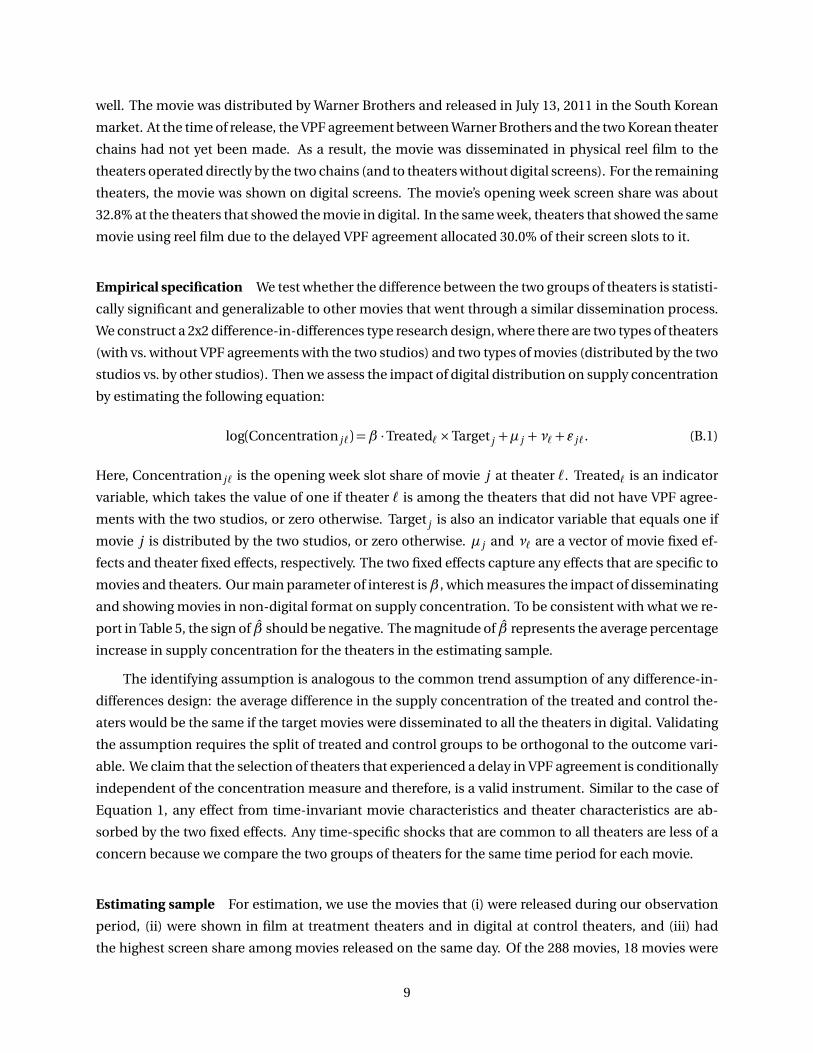
well. The movie was distributed by Warner Brothers and released in July 13, 2011 in the South Korean

market. At the time of release, the VPF agreement between Warner Brothers and the two Korean theater

chains had not yet been made. As a result, the movie was disseminated in physical reel film to the

theaters operated directly by the two chains (and to theaters without digital screens). For the remaining

theaters, the movie was shown on digital screens. The movie’s opening week screen share was about

32.8% at the theaters that showed the movie in digital. In the same week, theaters that showed the same

movie using reel film due to the delayed VPF agreement allocated 30.0% of their screen slots to it.

Empirical specification We test whether the difference between the two groups of theaters is statisti-

cally significant and generalizable to other movies that went through a similar dissemination process.

We construct a 2x2 difference-in-differences type research design, where there are two types of theaters

(with vs. without VPF agreements with the two studios) and two types of movies (distributed by the two

studios vs. by other studios). Then we assess the impact of digital distribution on supply concentration

by estimating the following equation:

log(Concentration j `) =β ·Treated`×Target j +µ j +ν`+ ε j `. (B.1)

Here, Concentration j ` is the opening week slot share of movie j at theater `. Treated` is an indicator

variable, which takes the value of one if theater ` is among the theaters that did not have VPF agree-

ments with the two studios, or zero otherwise. Target j is also an indicator variable that equals one if

movie j is distributed by the two studios, or zero otherwise. µ j and ν` are a vector of movie fixed ef-

fects and theater fixed effects, respectively. The two fixed effects capture any effects that are specific to

movies and theaters. Our main parameter of interest isβ , which measures the impact of disseminating

and showing movies in non-digital format on supply concentration. To be consistent with what we re-

port in Table 5, the sign of β̂ should be negative. The magnitude of β̂ represents the average percentage

increase in supply concentration for the theaters in the estimating sample.

The identifying assumption is analogous to the common trend assumption of any difference-in-

differences design: the average difference in the supply concentration of the treated and control the-

aters would be the same if the target movies were disseminated to all the theaters in digital. Validating

the assumption requires the split of treated and control groups to be orthogonal to the outcome vari-

able. We claim that the selection of theaters that experienced a delay in VPF agreement is conditionally

independent of the concentration measure and therefore, is a valid instrument. Similar to the case of

Equation 1, any effect from time-invariant movie characteristics and theater characteristics are ab-

sorbed by the two fixed effects. Any time-specific shocks that are common to all theaters are less of a

concern because we compare the two groups of theaters for the same time period for each movie.

Estimating sample For estimation, we use the movies that (i) were released during our observation

period, (ii) were shown in film at treatment theaters and in digital at control theaters, and (iii) had

the highest screen share among movies released on the same day. Of the 288 movies, 18 movies were

9

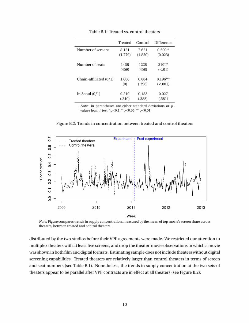
Table B.1: Treated vs. control theaters

Treated Control Difference

Number of screens 8.121 7.621 0.500∗∗

(1.779) (1.850) (0.023)

Number of seats 1438 1228 210∗∗∗

(459) (458) (<.01)

Chain-affiliated (0/1) 1.000 0.804 0.196∗∗∗

(0) (.398) (<.001)

In Seoul (0/1) 0.210 0.183 0.027(.210) (.388) (.581)

Note: in parentheses are either standard deviations or p -values from t test; ∗p<0.1; ∗∗p<0.05; ∗∗∗p<0.01.

Figure B.2: Trends in concentration between treated and control theaters

Note: Figure compares trends in supply concentration, measured by the mean of top movie’s screen share acrosstheaters, between treated and control theaters.

distributed by the two studios before their VPF agreements were made. We restricted our attention to

multiplex theaters with at least five screens, and drop the theater-movie observations in which a movie

was shown in both film and digital formats. Estimating sample does not include theaters without digital

screening capabilities. Treated theaters are relatively larger than control theaters in terms of screen

and seat numbers (see Table B.1). Nonetheless, the trends in supply concentration at the two sets of

theaters appear to be parallel after VPF contracts are in effect at all theaters (see Figure B.2).

10

Table B.2: Estimation results of the natural experiment

DV: Supply concentration (at theater-level)

(1) (2)w/ control movies (2) w/o control movies

Treated × Targetβ̂ 2011−16 −0.119∗∗∗

SE (0.028)

Treatedβ̂ 2011−16 −0.126∗∗∗

SE (0.031)

Movie FE Yes YesTheater FE Yes NoN 35,357 1,230R2 0.802 0.678Adj. R2 0.799 0.673

Note: Columns report estimated β in Equation B.1. Standard errors are clustered bytheaters; ∗p<0.1; ∗∗p<0.05; ∗∗∗p<0.01.

Results Table B.2 reports the estimation results of Equation B.1. The parameter estimate reported in

column (1) shows that the treated theaters allocated 11.9% fewer showings for the target movies than

the theaters in the control group. This is approximately an 0.025 decrease from the baseline supply

concentration of 0.21 of the control theaters for target movies. In column (2) we report the parameter

estimate without having control movies, based on the difference in outcomes between treated and

non-treated theaters only for target movies. The estimate is slightly greater (in absolute value) than

that in column (1), which demonstrates the importance of controlling for the average concentration

level between two groups using the difference-in-differences approach. In sum, Table B.2 suggests that

digitization supply movie concentration in the sample theaters.

Robustness: placebo tests As a robustness check for our findings regarding supply concentration in

Table B.2, we conduct two different placebo tests. First, we randomly draw a set of movies and assign

them as target movies and estimate Equation B.1, while fixing the split between treated and control

theaters. Second, while fixing the target movies, we randomly assign theaters to the treated or control

group and estimate the same equation. In each case, we draw the same number of true target or treated

theaters. We repeat the procedure 5,000 times. Figure B.3 in the Online Appendix shows the distribu-

tion of estimates. The graph shows that an estimate of −.119 from Table B.2, Equation B.1 is extremely

unlikely to have arisen by chance. The mean of these placebo test models is indistinguishable from

zero and our true estimate lies in the tail of the distributions.

11

Figure B.3: Distribution of placebo effects on supply concentration

Note: Figures report the kernel density for the distribution of 5,000 placebo estimates using randomly selectedmovie titles (left) or theaters (right). In each panel, the black solid line is a kernel density for the distribution ofplacebo estimates of the effect of digitization on supply concentration. The solid vertical lines are the mean ofeach distribution, where the dashed line is the true estimate from column (1) in Table B.2.

12

C Additional Figures and Tables

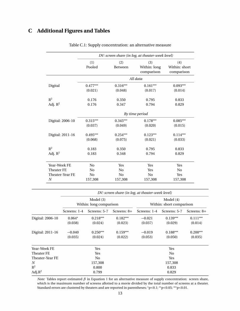
Table C.1: Supply concentration: an alternative measure

DV: screen share (in log, at theater-week level)

(1) (2) (3) (4)Pooled Between Within: long Within: short

comparison comparison

All data

Digital 0.477∗∗∗ 0.316∗∗∗ 0.161∗∗∗ 0.093∗∗∗

(0.021) (0.048) (0.017) (0.014)

R2 0.176 0.350 0.795 0.833Adj. R2 0.176 0.347 0.794 0.829

By time period

Digital: 2006-10 0.315∗∗∗ 0.345∗∗∗ 0.178∗∗∗ 0.085∗∗∗

(0.037) (0.049) (0.020) (0.015)

Digital: 2011-16 0.495∗∗∗ 0.254∗∗∗ 0.123∗∗∗ 0.114∗∗∗

(0.068) (0.075) (0.021) (0.033)

R2 0.183 0.350 0.795 0.833Adj. R2 0.183 0.348 0.794 0.829

Year-Week FE No Yes Yes YesTheater FE No No Yes NoTheater-Year FE No No No YesN 157,308 157,308 157,308 157,308

DV: screen share (in log, at theater-week level)

Model (3) Model (4)Within: long comparison Within: short comparison

Screens: 1-4 Screens: 5-7 Screens: 8+ Screens: 1-4 Screens: 5-7 Screens: 8+

Digital: 2006-10 0.064∗ 0.218∗∗∗ 0.182∗∗∗ −0.021 0.139∗∗∗ 0.111∗∗∗

(0.038) (0.024) (0.023) (0.037) (0.029) (0.014)

Digital: 2011-16 −0.040 0.250∗∗∗ 0.159∗∗∗ −0.019 0.188∗∗∗ 0.200∗∗∗

(0.035) (0.024) (0.022) (0.053) (0.050) (0.035)

Year-Week FE Yes YesTheater FE Yes NoTheater-Year FE No YesN 157,308 157,308R2 0.800 0.833Adj.R2 0.799 0.829

Note: Tables report estimated β in Equation 1 for an alternative measure of supply concentration: screen share,which is the maximum number of screens allotted to a movie divided by the total number of screens at a theater.Standard errors are clustered by theaters and are reported in parentheses; ∗p<0.1; ∗∗p<0.05; ∗∗∗p<0.01.

13

Figure C.1: An illustration of pre-trends in product variety and supply concentration

A. Product Variety

B. Supply concentration

Note: Figure compares pre-trends in product variety and supply concentration between one treated theater andits control theaters. The treated theater was converted in week 66 and we display its pre-trend (weeks 1-65) insolid lines. The dashed lines represent the average pre-trend of all control theaters (i.e., all other theaters thathad not adopted at the time the treated theater adopted). The pairwise correlation between the two time-seriesare 0.829 and 0.798, respectively.

14

Table C.2: Product variety: parallel trending theaters only

DV: product variety (in log, at theater-week level)



All data

Digital 0.147∗∗∗ −0.041 −0.150∗∗∗ −0.098∗∗∗

(0.027) (0.068) (0.023) (0.013)

R2 0.022 0.205 0.805 0.840Adj. R2 0.022 0.201 0.803 0.836

By time period

Digital: 2006-10 −0.012 −0.108 −0.205∗∗∗ −0.134∗∗∗

(0.054) (0.075) (0.027) (0.012)

Digital: 2011-16 0.192∗∗∗ 0.192∗∗ 0.041∗ 0.029(0.067) (0.076) (0.023) (0.030)

R2 0.030 0.208 0.806 0.840Adj. R2 0.030 0.203 0.805 0.836





Digital: 2006-10 −0.297∗∗ −0.136∗∗∗ −0.212∗∗∗ −0.067 −0.120∗∗∗ −0.144∗∗∗

(0.118) (0.029) (0.024) (0.047) (0.015) (0.016)

Digital: 2011-16 0.123 0.044∗ 0.027 0.135 0.061∗∗∗ −0.019(0.079) (0.025) (0.025) (0.187) (0.022) (0.048)


Note: Tables report estimated β in Equation 1 for product variety. We exclude the treated theaters with the pairwisecorrelation with its corresponding control theaters in the pre-adoption period is less than the sample median. Thesample median indicates the median value of the pairwise correlations across all treated theaters. Standard errorsare clustered by theaters and are reported in parentheses; ∗p<0.1; ∗∗p<0.05; ∗∗∗p<0.01.

15

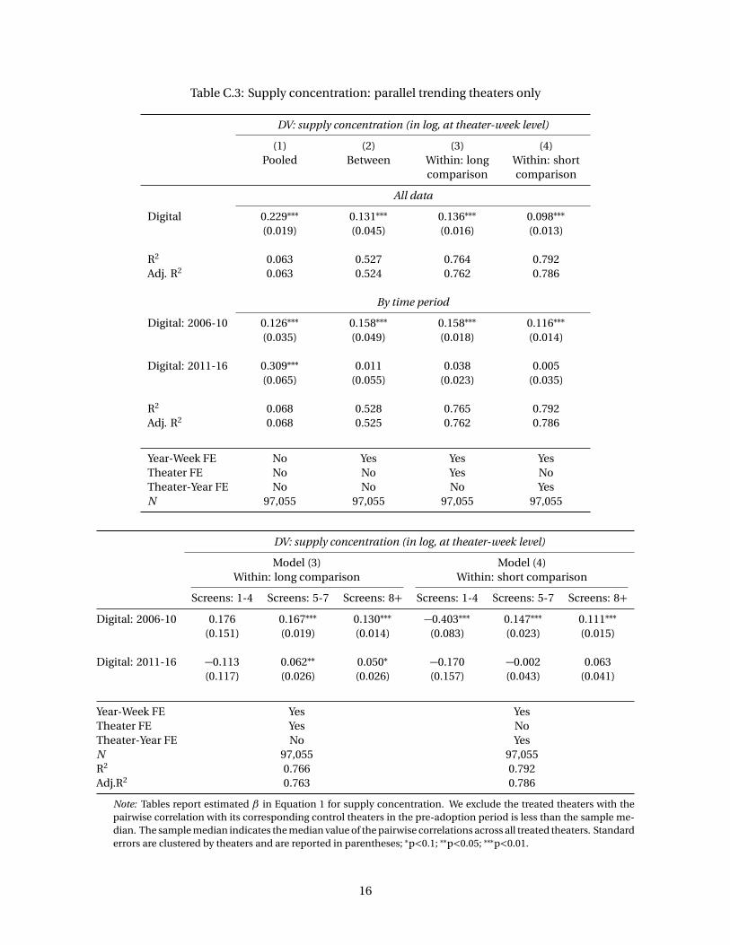
Table C.3: Supply concentration: parallel trending theaters only

DV: supply concentration (in log, at theater-week level)



All data

Digital 0.229∗∗∗ 0.131∗∗∗ 0.136∗∗∗ 0.098∗∗∗

(0.019) (0.045) (0.016) (0.013)

R2 0.063 0.527 0.764 0.792Adj. R2 0.063 0.524 0.762 0.786

By time period

Digital: 2006-10 0.126∗∗∗ 0.158∗∗∗ 0.158∗∗∗ 0.116∗∗∗

(0.035) (0.049) (0.018) (0.014)

Digital: 2011-16 0.309∗∗∗ 0.011 0.038 0.005(0.065) (0.055) (0.023) (0.035)

R2 0.068 0.528 0.765 0.792Adj. R2 0.068 0.525 0.762 0.786





Digital: 2006-10 0.176 0.167∗∗∗ 0.130∗∗∗ −0.403∗∗∗ 0.147∗∗∗ 0.111∗∗∗

(0.151) (0.019) (0.014) (0.083) (0.023) (0.015)

Digital: 2011-16 −0.113 0.062∗∗ 0.050∗ −0.170 −0.002 0.063(0.117) (0.026) (0.026) (0.157) (0.043) (0.041)


Note: Tables report estimated β in Equation 1 for supply concentration. We exclude the treated theaters with thepairwise correlation with its corresponding control theaters in the pre-adoption period is less than the sample me-dian. The sample median indicates the median value of the pairwise correlations across all treated theaters. Standarderrors are clustered by theaters and are reported in parentheses; ∗p<0.1; ∗∗p<0.05; ∗∗∗p<0.01.

16

Table C.4: Supply concentration by dayparts: daypart specific concentration

DV: supply concentration (in log, at theater-week-daypart level)

2006-10 2011-16

(1) (2) (3) (4) (5) (6)Screens: 1-4 5-7 8+ Screens: 1-4 5-7 8+

MTW daytime†

Digital −0.010 0.102∗∗∗ 0.110∗∗∗ −0.062∗∗ −0.034 0.008(0.027) (0.019) (0.016) (0.028) (0.032) (0.027)

MTW eveningDigital 0.010 0.170∗∗∗ 0.170∗∗∗ 0.025 0.067∗∗ 0.056∗

(0.031) (0.022) (0.016) (0.031) (0.029) (0.030)

Thursday-FridayDigital −0.011 0.111∗∗∗ 0.123∗∗∗ −0.042 0.031 0.059∗∗

(0.025) (0.019) (0.016) (0.027) (0.031) (0.026)

Weekend daytimeDigital −0.019 0.078∗∗∗ 0.105∗∗∗ −0.028 0.034 0.086∗∗∗

(0.022) (0.019) (0.016) (0.032) (0.033) (0.030)

Weekend eveningDigital 0.007 0.154∗∗∗ 0.170∗∗∗ 0.044 0.133∗∗∗ 0.124∗∗∗

(0.028) (0.022) (0.018) (0.037) (0.030) (0.031)

Year-Week FE Yes Yes Yes Yes Yes YesTheater-Year FE Yes Yes Yes Yes Yes YesTheater-Daypart FE Yes Yes Yes Yes Yes YesN 52,111 99,972 149,398 129,702 157,979 214,120R2 0.658 0.548 0.660 0.612 0.692 0.741Adj. R2 0.652 0.542 0.656 0.607 0.689 0.738

Note: Columns report estimated β in Equation 2 for supply concentration by time period and theatersize. Supply concentration is defined in each specific daypart. Standard errors are clustered by theatersand are reported in parentheses; ∗p<0.1; ∗∗p<0.05; ∗∗∗p<0.01.†MTW daytime (Monday to Wednesday all before 5 PM), MTW evening (Monday to Wednesday all after5 PM), Thursday-Friday (Thursday all day and Friday before 5 PM), Weekend daytime (Saturday before5PM and Sunday before 5 PM), and Weekend evening (Friday to Sunday all after 5PM).

17

Table C.5: Product variety by dayparts for Model 3

DV: product variety (in log, at theater-week-daypart level)

2006-10 2011-16

(1) (2) (3) (4) (5) (6)Screens: 1-4 5-7 8+ Screens: 1-4 5-7 8+

MTW daytime†

Digital −0.044 −0.160∗∗∗ −0.100∗∗∗ 0.196∗∗ 0.135∗∗∗ 0.064(0.037) (0.025) (0.022) (0.093) (0.026) (0.041)

MTW eveningDigital −0.059 −0.183∗∗∗ −0.128∗∗∗ 0.030 −0.039 −0.081∗

(0.037) (0.025) (0.023) (0.063) (0.028) (0.049)

Thursday-FridayDigital −0.047 −0.159∗∗∗ −0.116∗∗∗ 0.167∗ 0.072∗∗∗ 0.041

(0.033) (0.025) (0.023) (0.091) (0.024) (0.039)

Weekend daytimeDigital −0.046 −0.130∗∗∗ −0.083∗∗∗ 0.125∗ 0.056∗∗ −0.039

(0.035) (0.025) (0.022) (0.071) (0.026) (0.046)

Weekend eveningDigital −0.076∗∗ −0.192∗∗∗ −0.151∗∗∗ −0.023 −0.105∗∗∗ −0.158∗∗∗

(0.032) (0.024) (0.023) (0.059) (0.026) (0.052)


Note: Columns report estimated β in Equation 2 for product variety by time period and theater size. Standarderrors are clustered by theaters and are reported in parentheses; ∗p<0.1; ∗∗p<0.05; ∗∗∗p<0.01.†MTW daytime (Monday to Wednesday all before 5 PM), MTW evening (Monday to Wednesday all after 5PM), Thursday-Friday (Thursday all day and Friday before 5 PM), Weekend daytime (Saturday before 5PMand Sunday before 5 PM), and Weekend evening (Friday to Sunday all after 5PM).

18

Table C.6: Supply concentration by dayparts for Model 3

DV: supply concentration (in log, at theater-week-daypart level)

2006-10 2011-16

(1) (2) (3) (4) (5) (6)Screens: 1-4 5-7 8+ Screens: 1-4 5-7 8+

MTW daytime†

Digital 0.020 0.127∗∗∗ 0.081∗∗∗ −0.096∗ −0.055∗ −0.004(0.025) (0.025) (0.020) (0.056) (0.030) (0.033)

MTW eveningDigital 0.022 0.195∗∗∗ 0.140∗∗∗ −0.027 0.052∗∗ 0.054

(0.029) (0.026) (0.020) (0.054) (0.023) (0.035)

Thursday-FridayDigital 0.028 0.140∗∗∗ 0.099∗∗∗ −0.075 −0.005 0.033

(0.025) (0.024) (0.020) (0.063) (0.029) (0.033)

Weekend daytimeDigital −0.003 0.085∗∗∗ 0.049∗∗ −0.089 0.0002 0.086∗∗

(0.027) (0.025) (0.020) (0.055) (0.032) (0.038)

Weekend eveningDigital 0.037 0.177∗∗∗ 0.134∗∗∗ 0.006 0.121∗∗∗ 0.129∗∗∗

(0.024) (0.024) (0.022) (0.059) (0.027) (0.033)


Note: Columns report estimated β in Equation 2 for supply concentration by time period and theatersize. Supply concentration in each daypart is defined with respect to the movie that was mostly shownin a given theater-week. Standard errors are clustered by theaters and are reported in parentheses;∗p<0.1; ∗∗p<0.05; ∗∗∗p<0.01.†MTW daytime (Monday to Wednesday all before 5 PM), MTW evening (Monday to Wednesday all after5 PM), Thursday-Friday (Thursday all day and Friday before 5 PM), Weekend daytime (Saturday before5PM and Sunday before 5 PM), and Weekend evening (Friday to Sunday all after 5PM).

19

Figure C.2: Flexibility in within-week movie scheduling

Note: Figure reports trends in theaters’ weekly movie scheduling decisions. Definition of each vari-able is as follows: VARIETY is the number of different movies screened; CONCENTRATION is themaximum screen share of a movie; MINPLAY is the minimum number of slots for a movie; MAXSCRis the maximum number of screens for a movie; MLTMOVSCR is the number of screens that showedmultiple movies; MLTSCRMOV is the number of movies on multiple screens; and GINI is Gini coef-ficient of play counts. The black solid lines are smooth splines. As shown in the plots, theaters’ reac-tion to digital distribution stands out from the trends. In the main text, we discussed in depth aboutVARIETY and CONCENTRATION. Figure suggests that digitization-driven cost reduction also leadstheaters to more flexibly manage their screens, which decreases the minimum number of showsfor a movie (MINPLAY) to one and increasing the maximum number of screens a single title has(MAXSCR). Moreover, there are more screen that show multiple movies (MLTMOVSCR) and moremovies that are allocated to multiple screens (MLTSCRMOV) within a week. This has been possiblebecause there is increasing number of switch between titles at a screen (SWITCH). It is immediatethat the Gini index has increased given the changes in other variables.

20

Figure C.3: Flexibility in across-week movie scheduling

A. Distribution of screen numbers over time

Note: Figure reports the distribution of screen allocation (y-axis) by the number of days after release(x-axis) up to 40 days. Each line represents a percentile of the distribution over time.

B. Distribution of in-release days and closing types

Note: Figure compares the distribution of in-release days of movies. Only movies released on Thursdayare used (87% and 74% in 2006 and 2015, respectively). Weekly closing refers to the case where a movieclosed with in-release days of multiples of seven. The left panel shows the cumulative mass function ofin-release days for 2006 (blue line) and 2015 (red line) movies. Here, in-release days of a movie is definedas the number of days elapsed since its release until no theaters in the market allocate screens to it (notincluding re-releases).

21

Table C.7: Event-study specification estimation results: at theater-level

(1) (2) (3) (4) (5) (6) (7) (8) (9) (10) (11)-5 weeks -4 weeks -3 weeks -2 weeks -1 week 0 week 1 week 2 weeks 3 weeks 4 weeks 5 weeks


Digital: 2006-10 −0.020 −0.040∗∗ −0.040∗∗ −0.047∗∗ −0.057∗∗∗ −0.004 −0.036∗ −0.015 −0.009 −0.007 −0.013(0.015) (0.017) (0.019) (0.020) (0.022) (0.021) (0.022) (0.017) (0.015) (0.014) (0.013)

Digital: 2011-16 −0.087∗∗ −0.050 −0.039 −0.088∗∗ −0.133∗∗ 0.058 0.058 0.059 0.082∗∗ 0.122∗∗∗ 0.124∗∗∗

(0.037) (0.032) (0.036) (0.045) (0.061) (0.043) (0.064) (0.043) (0.039) (0.035) (0.032)

R2 0.815 0.817 0.821 0.830 0.841 0.868 0.858 0.847 0.842 0.833 0.821Adj. R2 0.792 0.792 0.794 0.799 0.807 0.813 0.800 0.802 0.805 0.802 0.793


Digital: screens 1-4 0.029 0.039 0.032 0.014 −0.021 −0.002 0.011 0.013 0.011 −0.008 −0.025(0.033) (0.033) (0.036) (0.051) (0.049) (0.054) (0.064) (0.058) (0.050) (0.043) (0.038)

Digital: screens 5-7 −0.012 −0.010 0.008 0.030 0.049 0.149∗∗∗ 0.203∗∗∗ 0.169∗∗∗ 0.119∗∗∗ 0.118∗∗∗ 0.114∗∗∗

(0.024) (0.027) (0.029) (0.028) (0.032) (0.050) (0.047) (0.037) (0.031) (0.031) (0.031)

Digital: screens 8+ 0.007 0.018 0.020 0.025 0.066∗∗ 0.049 0.162∗∗∗ 0.105∗∗∗ 0.079∗∗∗ 0.088∗∗∗ 0.088∗∗∗

(0.027) (0.032) (0.031) (0.027) (0.031) (0.035) (0.040) (0.034) (0.028) (0.026) (0.025)

R2 0.742 0.744 0.750 0.769 0.780 0.804 0.792 0.779 0.770 0.745 0.730Adj. R2 0.711 0.709 0.711 0.728 0.732 0.722 0.707 0.714 0.717 0.697 0.687

Theater FE Yes Yes Yes Yes Yes Yes Yes Yes Yes Yes YesN 2,365 2,135 1,902 1,669 1,439 1,700 1,684 2,157 2,628 3,097 3,567

Note: The table reports the results of event-study specification at theater-level. Columns (1)-(5): the estimates report the pre-trends in product variety andsupply concentration. We compute the mean difference in product variety or supply concentration between the period of n-weeks before adoption and the fivepreceding weeks. Columns (6)-(8): the estimates reports the mean difference between pre- and post-adoption in product variety and supply concentrationacross treated theaters. We use five preceding weeks before adoption as the pre-period and n weeks after adoption as post-period. Standard errors areclustered by theaters and are reported in parentheses; ∗p<0.1; ∗∗p<0.05; ∗∗∗p<0.01.

22

Table C.8: Event-study specification estimation results: at screen-level

(1) (2) (3) (4) (5) (6) (7) (8) (9) (10) (11)-5 weeks -4 weeks -3 weeks -2 weeks -1 week 0 week 1 week 2 weeks 3 weeks 4 weeks 5 weeks

DV: product variety (in log, at screen-level)

Digital: 2006-10 0.021 0.009 −0.004 −0.023 −0.024 0.146∗∗∗ −0.002 0.001 0.022 0.032∗∗ 0.037∗∗

(0.015) (0.014) (0.015) (0.016) (0.020) (0.021) (0.021) (0.017) (0.016) (0.016) (0.016)

Digital: 2011-16 0.010 0.055∗∗∗ 0.054∗∗ 0.018 −0.001 0.260∗∗∗ 0.174∗∗∗ 0.182∗∗∗ 0.181∗∗∗ 0.204∗∗∗ 0.216∗∗∗

(0.021) (0.021) (0.023) (0.024) (0.028) (0.030) (0.033) (0.028) (0.025) (0.024) (0.022)

R2 0.434 0.447 0.463 0.479 0.496 0.495 0.496 0.466 0.443 0.427 0.417Adj. R2 0.364 0.370 0.377 0.382 0.382 0.379 0.379 0.364 0.352 0.346 0.344

DV: number of switches (at screen-level)

Digital: 2006-10 −0.227 0.005 0.053 0.155 0.198 0.630∗∗ 0.045 0.199 0.078 0.230 0.350∗

(0.181) (0.196) (0.200) (0.228) (0.299) (0.284) (0.274) (0.242) (0.212) (0.203) (0.191)

Digital: 2011-16 −0.258 0.026 0.134 0.104 0.631∗ 1.453∗∗∗ 1.912∗∗∗ 2.209∗∗∗ 2.335∗∗∗ 2.569∗∗∗ 2.691∗∗∗

(0.256) (0.262) (0.279) (0.309) (0.383) (0.381) (0.458) (0.375) (0.334) (0.328) (0.314)

R2 0.414 0.425 0.434 0.453 0.472 0.457 0.461 0.436 0.414 0.405 0.396Adj. R2 0.342 0.344 0.344 0.351 0.354 0.333 0.337 0.328 0.319 0.321 0.320

Theater-Screen FE Yes Yes Yes Yes Yes Yes Yes Yes Yes Yes YesN 15,744 14,126 12,522 10,910 9,304 9,456 9,366 11,010 12,633 14,239 15,822

Notes: The upper panel reports the changes in product variety after digital transition of a screen. In the lower panel, we report the changes in the numberof switches between movies. Specifically, we construct an outcome variable, Switch, which measures per screen-week frequency of switches betweenmovies within a screen-day. That is, if a theater shows movie A in a screen only during the daytime slots and switches to movie B for the evening slotsthroughout a week, then Switch= 7. Columns (1)-(5): the estimates report the pre-trends in product variety and Switch. We compute the mean differencein product variety or Switch between the period of n-weeks before adoption and the five preceding weeks. Columns (6)-(11): the estimates reports the meandifference between pre- and post-adoption in product variety and Switch across treated theater-screens. We use five preceding weeks before adoption asthe pre-period and n weeks after adoption as post-period. Standard errors are clustered standard errors by theaters are reported in parentheses; ∗p<0.1;∗∗p<0.05; ∗∗∗p<0.01.

23

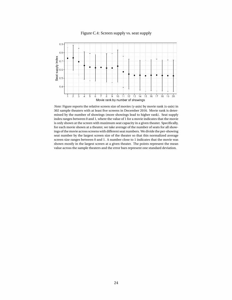
Figure C.4: Screen supply vs. seat supply

Note: Figure reports the relative screen size of movies (y-axis) by movie rank (x-axis) in302 sample theaters with at least five screens in December 2016. Movie rank is deter-mined by the number of showings (more showings lead to higher rank). Seat supplyindex ranges between 0 and 1, where the value of 1 for a movie indicates that the movieis only shown at the screen with maximum seat capacity in a given theater. Specifically,for each movie shown at a theater, we take average of the number of seats for all show-ings of the movie across screens with different seat numbers. We divide the per-showingseat number by the largest screen size of the theater so that this normalized averagescreen size ranges between 0 and 1. A number close to 1 indicates that the movie wasshown mostly in the largest screen at a given theater. The points represent the meanvalue across the sample theaters and the error bars represent one standard deviation.

24

Table C.9: Additional estimation results of the natural experiment

(1) (2)Run length (weeks) Total concentration

(at theater-level) (at theater-level)

Target × treated −0.080 −0.076∗∗∗

(0.060) (0.018)

Movie FE Yes YesTheater FE Yes YesObservations 35,357 35,357R2 0.841 0.899Adjusted R2 0.838 0.897

Note: The table reports two additional estimation results from thenatural experiment. The same dataset as in Table B.2 is used.The clustered standard errors at the theater-level are reported inparentheses; ∗p<0.1; ∗∗p<0.05; ∗∗∗p<0.01.

25

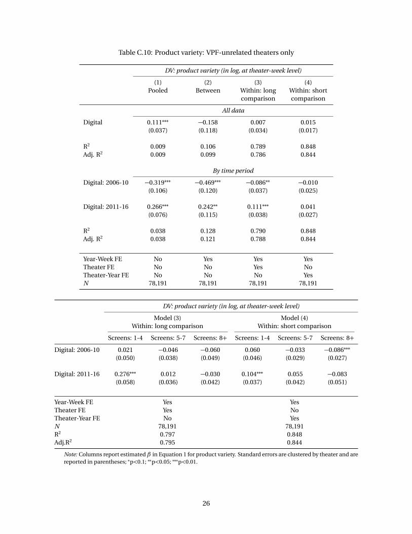
Table C.10: Product variety: VPF-unrelated theaters only




All data

Digital 0.111∗∗∗ −0.158 0.007 0.015(0.037) (0.118) (0.034) (0.017)

R2 0.009 0.106 0.789 0.848Adj. R2 0.009 0.099 0.786 0.844

By time period

Digital: 2006-10 −0.319∗∗∗ −0.469∗∗∗ −0.086∗∗ −0.010(0.106) (0.120) (0.037) (0.025)

Digital: 2011-16 0.266∗∗∗ 0.242∗∗ 0.111∗∗∗ 0.041(0.076) (0.115) (0.038) (0.027)

R2 0.038 0.128 0.790 0.848Adj. R2 0.038 0.121 0.788 0.844





Digital: 2006-10 0.021 −0.046 −0.060 0.060 −0.033 −0.086∗∗∗

(0.050) (0.038) (0.049) (0.046) (0.029) (0.027)

Digital: 2011-16 0.276∗∗∗ 0.012 −0.030 0.104∗∗∗ 0.055 −0.083(0.058) (0.036) (0.042) (0.037) (0.042) (0.051)


Note: Columns report estimated β in Equation 1 for product variety. Standard errors are clustered by theater and arereported in parentheses; ∗p<0.1; ∗∗p<0.05; ∗∗∗p<0.01.

26

online appendix for digitization and flexibility: evidence

Documents