One More Bit Is Enough

Yong Xia∗ Lakshminarayanan Subramanian+ Ion Stoica+ Shivkumar Kalyanaraman∗

∗ ECSE Department + EECS DepartmentRensselaer Polytechnic Institute University of California, Berkeley

{xiay@alum, shivkuma@ecse}.rpi.edu {lakme, istoica}@cs.berkeley.edu

ABSTRACTAchieving efficient and fair bandwidth allocation while min-imizing packet loss in high bandwidth-delay product net-works has long been a daunting challenge. Existing end-to-end congestion control (e.g., TCP) and traditional con-gestion notification schemes (e.g., TCP+AQM/ECN) havesignificant limitations in achieving this goal. While the re-cently proposed XCP protocol addresses this challenge, XCPrequires multiple bits to encode the congestion-related infor-mation exchanged between routers and end-hosts. Unfortu-nately, there is no space in the IP header for these bits,and solving this problem involves a non-trivial and time-consuming standardization process.

In this paper, we design and implement a simple, low-complexity protocol, called Variable-structure congestionControl Protocol (VCP), that leverages only the existing twoECN bits for network congestion feedback, and yet achievescomparable performance to XCP, i.e., high utilization, lowpersistent queue length, negligible packet loss rate, and rea-sonable fairness. On the downside, VCP converges signifi-cantly slower to a fair allocation than XCP. We evaluate theperformance of VCP using extensive ns2 simulations over awide range of network scenarios. To gain insight into the be-havior of VCP, we analyze a simple fluid model, and provea global stability result for the case of a single bottlenecklink shared by flows with identical round-trip times.

Categories and Subject DescriptorsC.2.2 [Computer-Communication Networks]: Network Protocols

General TermsAlgorithms, Design, Experimentation, Performance, Theory

KeywordsCongestion Control, Protocol, TCP, AQM, ECN, XCP

1. INTRODUCTIONThe Additive-Increase-Multiplicative-Decrease (AIMD) [10]

congestion control algorithm employed by TCP [25] is known

Permission to make digital or hard copies of all or part of this work forpersonal or classroom use is granted without fee provided that copies arenot made or distributed for profit or commercial advantage and that copiesbear this notice and the full citation on the first page. To copy otherwise, torepublish, to post on servers or to redistribute to lists, requires prior specificpermission and/or a fee.SIGCOMM’05,August 21–26, 2005, Philadelphia, Pennsylvania, USA.Copyright 2005 ACM 1-59593-009-4/05/0008 ...$5.00.

to be ill-suited for high Bandwidth-Delay Product (BDP)networks. With rapid advances in the deployment of veryhigh bandwidth links in the Internet, the need for a viablereplacement of TCP in such environments has become in-creasingly important.

Several research efforts have proposed different approachesfor this problem, each with their own strengths and limita-tions. These can be broadly classified into two categories:end-to-end and network feedback based approaches. Pureend-to-end congestion control schemes such as HighSpeedTCP [15], FAST [31] and BIC [67, 59], although being at-tractive solutions for the short-term (due to a lesser deploy-ment barrier), may not be suitable as long-term solutions.Indeed, in high BDP networks, using loss and/or delay asthe only congestion signal(s) poses fundamental limitationson achieving high utilization and fairness while maintain-ing low bottleneck queue length and minimizing congestion-induced packet drop rate. HighSpeed TCP illustrates thelimitations of loss-based approaches in high bandwidth op-tical links with very low bit-error rates [15]. Similarly, ithas been shown that delay-based approaches are highly sen-sitive to minor delay variations [7], a common case in today’sInternet.

To address some of the limitations of end-to-end con-gestion control schemes, many researchers have proposedthe use of explicit network feedback. However, while tra-ditional congestion notification feedback schemes such asTCP+AQM/ECN proposals [18, 2, 42, 57] are successfulin reducing the loss rate and the queue size in the network,they still fall short in achieving high utilization in high BDPnetworks [24, 49, 35]. XCP [35] addresses this problem byhaving routers estimate the fair rate and send this rate backto the senders. Congestion control schemes that use explicitrate feedback have been also proposed in the context of theATM Available Bit Rate (ABR) service [40, 9, 33, 27, 34].However, these schemes are hard to deploy in today’s Inter-net as they require a non-trivial number of bits to encodethe rate, bits which are not available in the IP header.

In this paper, we show that it is possible to approximateXCP’s performance in high BDP networks by leveragingonly the two ECN bits (already present in the IP header)to encode the congestion feedback. The crux of our algo-rithm, called Variable-structure congestion Control Proto-col (VCP), is to dynamically adapt the congestion controlpolicy as a function of the level of congestion in the net-work. With VCP, each router computes a load factor [27],and uses this factor to classify the level of congestion intothree regions: low-load, high-load and overload [28]. The

1

router encodes the level of congestion in the ECN bits. Aswith ECN, the receiver sends the congestion information tothe sender via acknowledgement (ACK) packets. Based onthe load region reported by the network, the sender usesone of the following policies: Multiplicative Increase (MI) inthe low-load region, Additive Increase (AI) in the high-loadregion, and Multiplicative Decrease (MD) in the overloadregion. By using MI in the low-load region, flows can ex-ponentially ramp up their bandwidth to improve networkutilization. Once high utilization is attained, AIMD pro-vides long-term fairness amongst the competing flows.

Using extensive packet-level ns2 [52] simulations that covera wide range of network scenarios, we show that VCP canapproximate the performance of XCP by achieving high uti-lization, low persistent queue length, negligible packet droprate and reasonable fairness. One limitation of VCP (as isthe case for other end-host based approaches including TCPand TCP+AQM) is that it converges significantly slower toa fair allocation than XCP.

To better understand VCP, we analyze its stability andfairness properties using a simplified fluid model that ap-proximates VCP’s behavior. For the case of a single bottle-neck link shared by flows with identical round-trip delays, weprove that the model asymptotically achieves global stabil-ity independent of the link capacity, the feedback delay andthe number of flows. For more general multiple-bottlenecktopologies, we show that the equilibrium rate allocation ofthis model is max-min fair [4]. While this model may notaccurately reflect VCP’s dynamics, it does reinforce the sta-bility and fairness properties that we observe in our simula-tions and provides a good theoretical grounding for VCP.

From a practical point of view VCP has two advantages.First, VCP does not require any modifications to the IPheader since it can reuse the two ECN bits in a way that iscompatible with the ECN proposal [57]. Second, it is a sim-ple protocol with low algorithmic complexity. The complex-ity of VCP’s end-host algorithm is similar to that of TCP.The router algorithm maintains no per-flow state, and it hasvery low computation complexity. We believe that thesebenefits largely offset VCP’s limitation of having a muchslower fairness convergence speed than XCP.

The rest of the paper is organized as follows. In Section 2,we describe the guidelines that motivate the design of VCPand in Section 3, we provide a detailed description of VCP.In Section 4, we evaluate the performance of VCP using ex-tensive simulations. In Section 5, we develop a fluid modelthat approximates VCP’s behavior and characterize its sta-bility, fairness and convergence properties (with the detailedproofs presented in a technical report [66]). Section 6 ad-dresses concerns on the stability of VCP under heteroge-neous delays and the influence of switching between MI, AIand MD on efficiency and fairness. We review related workin Section 7 and summarize our findings in Section 8.

2. FOUNDATIONSIn this section, we first review why XCP scales to high

BDP networks while TCP+AQM does not. Then, we presenttwo guidelines that form the basis of the VCP design.

2.1 Why XCP outperforms TCP+AQM?There are two main reasons of why TCP does not scale

to high BDP networks. First, packet loss is a binary con-gestion signal that conveys no information about the degree

of congestion. Second, due to stability reasons, relying onlyon packet loss for congestion indication requires TCP to usea conservative window increment policy and an aggressivewindow decrement policy [25, 35]. In high BDP networks,every loss event forces a TCP flow to perform an MD, fol-lowed by the slow convergence of the AI algorithm to reachhigh utilization. Since the time for each individual AIMDepoch is proportional to the per-flow BDP, TCP flows re-main in low utilization regions for prolonged periods of timethereby resulting in poor link utilization. Using AQM/ECNin conjunction with TCP does not solve this problem sincethe (one-bit) ECN feedback, similar to a packet loss, is notindicative of the degree of congestion either.

XCP addresses this problem by precisely measuring thefair share of a flow at a router and providing explicit ratefeedback to end-hosts. One noteworthy aspect of XCP is thedecoupling of efficiency control and fairness control at eachrouter. XCP uses MIMD to control the flow aggregate andconverge exponentially fast to any available bandwidth anduses AIMD to fairly allocate the bandwidth among compet-ing flows. XCP, however, requires multiple bits in the packetheader to carry bandwidth allocation information (∆cwnd)from network routers to end-hosts, and congestion window(cwnd) and Round-Trip Time (RTT) information (rtt) fromthe end-hosts to the network routers.

2.2 Design Guidelines for VCPThe main goal of our work is to develop a simple con-

gestion control mechanism that can scale to high BDP net-works. By “simple” we mean an AQM-style approach whererouters merely provide feedback on the level of network con-gestion, and end-hosts perform congestion control actionsusing this feedback. Furthermore, to maintain the com-patibility with the existing IP header format, we restrictourselves to using only two bits to encode the congestion in-formation. To address these challenges, our solution buildsaround two design guidelines:

#1, Decouple efficiency control & fairness control.

Like XCP, VCP decouples efficiency and fairness control.However, unlike XCP where routers run the efficiency andfairness control algorithms and then explicitly communicatethe rate to end-hosts, VCP routers compute only a con-gestion level, and end-hosts run one of the two algorithmsas a function of the congestion level. More precisely, VCPclassifies the network utilization into different utilization re-gions [28] and determines the controller that is suitable fora given region. Efficiency and fairness have different levelsof relative importance in different utilization regions. Whennetwork utilization is low, the goal of VCP is to improveefficiency more than fairness. On the other hand, whenutilization is high, VCP accords higher priority to fairnessthan efficiency. By decoupling these two issues, end-hostshave only a single objective in each region and thus needto apply only one congestion response. For example, onesuch choice of congestion response, which we use in VCP,is to perform MI in low utilization regions for improving ef-ficiency, and to apply AIMD in high utilization regions forachieving fairness. The goal then is to switch between thesetwo congestion responses depending on the level of networkutilization.

#2, Use link load factor as the congestion signal.

XCP uses spare bandwidth (the difference between capac-

2

0

5

10

15

20

0 50 100 150 200 250

Flow T

hrough

put (M

bps)

Time (sec)

capacity1st flow2nd flow

Figure 1: The throughput dynamics of two flows of the

same RTT (80ms). They share one bottleneck with the

capacity bouncing between 10Mbps and 20Mbps. This

simple example unveils VCP’s potential to quickly track

changes in available bandwidth (with load-factor guided

MIMD) and thereafter achieve a fair bandwidth alloca-

tion (with AIMD).

ity and demand) as a measure of the degree of congestion.In VCP, we use load factor as the congestion signal, i.e., therelative ratio of demand and capacity [27].

While the load factor conveys less information than sparebandwidth, the fact that the load factor is a scale-free pa-rameter allows us to encode it using a small number of bitswithout much loss of information. In this paper, we showthat a two-bit encoding of the load factor is sufficient toapproximate XCP’s performance. Note that in comparisonto binary congestion signals such as loss and one-bit ECN,the load factor conveys more information about the degreeof network congestion.

2.3 A Simple IllustrationIn this subsection, we give a high level description of VCP

using a simple example. A detailed description of VCP ispresented in Section 3. Periodically, each router measuresthe load factor for its output links and classifies the loadfactor into three utilization regions: low-load, high-load oroverload. Each router encodes the utilization regions in thetwo ECN bits in the IP header of each data packet. In turn,the receiver sends back this information to the sender viathe ACK packets. Depending on this congestion informa-tion, the sender applies different congestion responses. Ifthe router signals low-load, the sender increases its sendingrate using MI; if the router signals high-load, the sender in-creases its sending rate using AI; otherwise, if the routersignals overload, the sender reduces its sending rate usingMD. The core of the VCP protocol is summarized by thefollowing pseudo code.

1) Each router periodically estimates a load factor, andencodes this load factor into the data packets’ IP header.This information is then sent back by the receiver to thesender via ACK packets.

2) Based on the load factor it receives, each sender per-forms one of the following control algorithms:

2.1) For low-load, perform MI;2.2) For high-load, perform AI;2.3) For overload, perform MD.

Figure 1 shows the throughput dynamics of two flows shar-ing one bottleneck link. Clearly, VCP is successful in track-ing the bandwidth changes by using MIMD, and achieve fairallocation when the second flow arrives, by using AIMD.

The Internet, however, is much more complex than thissimplified example across many dimensions: the link capac-ities and router buffer sizes are highly heterogeneous, theRTT of flows may differ significantly, and the number offlows is unknown and changes over time. We next describethe details of the VCP protocol, which will be able to handlemore realistic environments.

3. THE VCP PROTOCOLIn this section, we provide a detailed description of VCP.

We begin by presenting three key issues that need to beaddressed in the design of VCP. Then, we describe how weaddress each of these issues in turn.

3.1 Key Design IssuesTo make VCP a practical approach for the Internet-like

environments with significant heterogeneity in link capaci-ties, end-to-end RTTs, router buffer sizes and variable trafficcharacteristics, we need to address the following three keyissues.

Load factor transition point: VCP separates the net-work load condition into three regions: low-load, high-loadand overload. The load factor transition point in VCP rep-resents the boundary between the low-load and high-loadregions, which is also the demarcation between applying MIand AI algorithms. The choice of the transition point repre-sents a trade-off between achieving high link utilization andresponsiveness to congestion. Achieving high network uti-lization requires a high value for the transition point. Butthis choice negatively impacts responsiveness to congestion,which in turn affects the convergence time to achieve fair-ness. Additionally, given that Internet traffic is inherentlybursty [46][56], we require a reliable estimation algorithm ofthe load factor. We discuss the issue of load factor estima-tion in Section 3.2.

Setting of congestion control parameters: Using MIfor congestion control is often fraught with the danger of in-stability due to its large variations over short time scales.To maintain stability and avoid large queues at routers, weneed to make sure that the aggregate rate of the VCP flowsusing MI does not overshoot the link capacity. Similarly, toachieve fairness, we need to make sure that a flow enters theAI phase before the link gets congested. In order to sat-isfy these criteria, we need an appropriate choice of MI, AIand MD parameters that can achieve high utilization whilemaintaining stability, fairness and small persistent queues.To better understand these issues, we first describe our pa-rameter settings for a simplified network model, where allflows have the same RTT and observe the same state ofthe network load condition, i.e., all flows obtain the sameload factor feedback (Section 3.3). We then generalize ourparameter choice for flows with heterogeneous RTTs.

Heterogeneous RTTs: When flows have heterogeneousRTTs, different flows can run different algorithms (i.e., MI,AI, or MD) at a given time. This may lead to unpredictablebehavior. The RTT heterogeneity can have a significantimpact even when all flows run the same algorithm, if thisalgorithm is MI. In this case, a flow with a lower RTT canclaim much more bandwidth than a flow with a higher RTT.To address this problem, end-hosts need to adjust their MIparameters according to their observed RTTs, as discussedin Section 3.4.

3

cρl

^

ρl

lρ

00

(11)2

>100%

(10)2

80% 100%

80%

100%

: (01)2

code

load: low high over

Figure 2: The quantized load factor ρl at a link l is a

non-decreasing function of the raw load factor ρl and can

be represented by a two-bit code ρcl .

We now discuss these three design issues in greater detail.

3.2 Load Factor Transition PointConsider a simple scenario involving a fixed set of long-

lived flows. The goal of VCP is to reach a steady statewhere the system is near full utilization, and the flows useAIMD for congestion control. To achieve this steady state,the choice of the load factor transition point should satisfythree constraints:

• The transition point should be sufficiently high to en-able the system to obtain high overall utilization;

• After the flows perform an MD from an overloadedstate, the MD step should force the system to alwaysenter the high-load state, not the low-load state;

• If the utilization is marginally lower than the transitionpoint, a single MI step should only lift the system intothe high-load state, but not the overload state.

Let β < 1 denote the MD factor, i.e., when using the MDalgorithm, the sender reduces the congestion window withthe factor β (as in Equation (4) in Section 3.3). The firstconstraint requires a high transition point. This choice cou-pled with the second condition leads to a high value of β.However, a very high value of β is undesirable as it decreasesVCP’s response to congestion. For example, if the transi-tion point is 95%, then β > 0.95, and it takes VCP about 14RTTs to halve the congestion window. At the other end, ifwe chose β = 0.5 (as in TCP [25]), the transition point canbe at most 50%, which reduces the overall network utiliza-tion. To balance these conflicting requirements, we choseβ = 0.875, the same value used in the DECbit scheme [58].Given β, we set the load factor transition point to 80%.This gives us a “safety margin” of 7.5%, which allows thesystem to operate in the AIMD mode in steady state. Insummary, we choose the following three ranges to encodethe load factor ρl (see Figure 2):

• Low-load region: ρl = 80% when ρl ∈ [0%, 80%);

• High-load region: ρl = 100% when ρl ∈ [80%, 100%);

• Overload region: ρl > 100% when ρl ∈ [100%,∞).

Thus, the quantized load factor ρl can be represented us-ing a two-bit code ρc

l , i.e., ρcl = (01)2, (10)2 and (11)2 for

ρl = 80%, ρl = 100% and ρl > 100%, respectively. Thecode (00)2 is reserved for ECN-unaware source hosts to sig-nal “not-ECN-capable-transport” to ECN-capable routers,which is essential for incremental deployment [57]. The en-coded load factor is embedded in the two-bit ECN field inthe IP header.

Estimation of the load factor: Due to the bursty na-ture of the Internet traffic, we need to estimate the loadfactor over an appropriate time interval, tρ. When choos-ing tρ we need to balance two conflicting requirements. Onone hand, tρ should be larger than the RTTs experienced bymost flows to factor out the burstiness induced by the flows’responses to congestion. On the other hand, tρ should besmall enough to avoid queue buildup. Internet measure-ments [55, 30] report that roughly 75%∼90% of flows haveRTTs less than 200 ms. Hence, we set tρ = 200ms. Duringevery time interval tρ, each router estimates a load factor ρl

for each of its output links l as [27, 34, 18, 2, 42]:

ρl =λl + κq · ql

γl · Cl · tρ. (1)

Here, λl is the amount of input traffic during the period tρ, ql

is the persistent queue length during this period, κq controlshow fast the persistent queue drains [18, 2] (we set κq = 0.5),γl is the target utilization [42] (set to a value close to 1), andCl is the link capacity. The input traffic λl is measured usinga packet counter. To measure the persistent queue ql, we usea low-pass filter that samples the instantaneous queue size,q(t), every tq ¿ tρ (we chose tq = 10ms).

3.3 Congestion Control Parameter SettingIn this section, we discuss the choice of parameters used by

VCP to implement the MI/AI/MD algorithms. To simplifythe discussion, we consider a single link shared by flows,whose RTTs are equal to the link load factor estimationperiod, i.e., rtt = tρ. Hence, the flows have synchronousfeedback and their control intervals are also in sync withthe link load factor estimation. We will discuss the case ofheterogeneous RTTs in Section 3.4.

At any time t, a VCP sender performs one of the threeactions based on the value of the encoded load factor sentby the network:

MI : cwnd(t + rtt) = cwnd(t)× ( 1 + ξ ) (2)

AI : cwnd(t + rtt) = cwnd(t) + α (3)

MD : cwnd(t + δt) = cwnd(t)× β (4)

where rtt = tρ, δt → 0+, ξ > 0, α > 0 and 0 < β < 1. Basedon the relationship between the choice of the load factortransition point and the MD parameter β, we chose β =0.875 (see Section 3.2). We use α = 1.0 as is in TCP [25].

Setting the MI parameter: The stability of VCP isdictated by the MI parameter ξ. In network-based rate al-location approaches like XCP, the rate increase of a flow atany time is proportional to the spare capacity available inthe network [35]. Translating this into the VCP context, werequire the MI of the congestion window to be proportionalto 1 − ρl where ρl represents the current load factor. Dur-ing the MI phase, the current sending rate of each flow isproportional to the current load factor ρl. Consequently, weobtain

ξ(ρ) = κ · 1− ρl

ρl, (5)

where κ is a constant that determines the stability of VCPand controls the speed to converge toward full utilization.Based on analyzing the stability properties of this algorithm(see Theorem 1 in Section 5), we set κ = 0.25. Since end-

4

hosts only obtain feedback on the utilization region as op-posed to the exact value of the load factor, they need tomake a conservative assumption that the network load isnear the transition point. Thus, the end-hosts use the valueof ξ(80%) = 0.0625 in the MI phase.

3.4 Handling RTT Heterogeneity withParameter Scaling

Until now, we have considered the case where competingflows have the same RTT, and this RTT is also equal to theload factor estimation interval, tρ. In this section, we relaxthese assumptions by considering flows with heterogeneousRTTs. To offset the impact of the RTT heterogeneity, weneed to scale the congestion control parameters used by theend-hosts according to their RTTs.

Scaling the MI/AI parameters: Consider a flow witha round trip time rtt, and assume that all the routers use thesame interval, tρ, to estimate the load factor on each link.Let ξ and α represent the unscaled MI and AI parametersas described in Section 3.3, where all flows have an identicalRTT (= tρ). To handle the case of flows with different RTTs,we set the scaled MI/AI parameters ξs and αs as follows: 1

For MI : ξs ← (1 + ξ)rtttρ − 1 , (6)

For AI : αs ← α · rtt

tρ. (7)

An end-host uses the scaled parameters ξs and αs in (2)and (3) to adjust the congestion window after each RTT.The scaling of these parameters emulates the behavior of allflows having an identical RTT, which is equal to tρ. Thenet result is that over any time period, the window increaseunder either MI or AI is independent of the flows’ RTTs.Thus, unlike TCP, VCP flow’s throughput is not affected bythe RTT heterogeneity [44, 53, 16].

Handling MD: MD is an impulse-like operation that isnot affected by the length of the RTT. Hence, the value ofβ in (4) needs not to be scaled with the RTT of the flow.However, to avoid over reaction to the congestion signal, aflow should perform an MD at most once during an estima-tion interval tρ. Upon getting the first load factor feedbackthat signals congestion (i.e., ρc

l = (11)2), the sender imme-diately reduces its congestion window cwnd using MD, andthen freezes the cwnd for a time period of tρ. After thisperiod, the end-host runs AI for one RTT in order to obtainthe new load factor.

Scaling for fair rate allocation: RTT-based parameterscaling, as described above, only ensures that the congestionwindows of two flows with different RTTs converge to thesame value in steady state. However, this does not guaranteefairness as the rate of the flow is still inversely proportionalto its RTT, i.e., rate = cwnd/rtt. To achieve fair rateallocation, we need to add an additional scaling factor to theAI algorithm. To illustrate why this is the case, consider thesimple AIMD control mechanism applied to two competingflows where each flow i (= 1, 2) uses a separate AI parameterαi but a common MD parameter β. At the end of the M -th

1Equation (6) is the solution for 1 + ξ = (1 + ξs)tρrtt where the

right-hand side is the MI amount of a flow with the RTT valuertt, during a time interval tρ. Similarly, Equation (7) is obtained

by solving 1 + α = 1 +tρ

rttαs.

Table 1: VCP Parameter Setting

Para Value Meaning

tρ 200 ms the link load factor measurement interval

tq 10 ms the link queue sampling interval

γl 0.98 the link target utilization

κq 0.5 how fast to drain the link steady queue

κ 0.25 how fast to probe the available bw (MI)

α 1.0 the AI parameter

β 0.875 the MD parameter

congestion epoch that includes n > 1 rounds of AI and oneround of MD in each epoch, we have

cwndi(M) = β · [ cwndi(M − 1) + n · αi ].

Eventually, each flow i achieves a congestion window thatis proportional to its AI parameter, αi. Indeed, the ratio ofthe congestion windows of the two flows approaches α1/α2

for large values of M , and n > 1:

cwnd1(M)

cwnd2(M)=

cwnd1(M − 1)/n + α1

cwnd2(M − 1)/n + α2

=cwnd1(M − 2)/n2 + α1/n + α1

cwnd2(M − 2)/n2 + α1/n + α2

= · · · → α1

α2.

Hence, to allocate bandwidth fairly among two flows, weneed to scale each flow’s AI parameter αi using its own RTT.For this purpose, we use tρ as a common-base RTT for all theflows. Thus, the new AI scaling parameter, αrate, becomes

For AI : αrate ← αs · rtt

tρ= α · (rtt

tρ)2. (8)

3.5 Summary of ParametersTable 1 summarizes the set of VCP router/end-host pa-

rameters and their typical values. We note that throughoutall the simulations reported in this paper, we use the sameparameter values. This suggests that VCP is robust in alarge variety of environments.

4. PERFORMANCE EVALUATIONIn this section, we use extensive ns2 simulations to evalu-

ate the performance of VCP for a wide range of network sce-narios [19] including varying the link capacities in the range[100Kbps, 5Gbps], round trip times in the range [1ms, 1.5s],numbers of long-lived, FTP-like flows in the range [1, 1000],and arrival rates of short-lived, web-like flows in the range[1s−1, 1000s−1]. We always use two-way traffic with conges-tion resulted in the reverse path. The bottleneck buffer sizeis set to the bandwidth-delay product, or two packets perflow, whichever is larger. The data packet size is 1000 bytes,while the ACK packet is 40 bytes. All simulations are runfor at least 120s to ensure that the system has reached itssteady state. The average utilization statistics neglect thefirst 20% of simulation time. For all the time-series graphs,utilization and throughput are averaged over 500ms inter-val, while queue length and congestion window are sampledevery 10ms. We use a fixed set of VCP parameters listed inTable 1 for all the simulations in this paper.

5

0.6

0.7

0.8

0.9

1.0

1.1

0.1 1 10 100 1000

Bottle

neck

Utili

zatio

n

Bottleneck Capacity (Mbps)

VCP UtilizationXCP Utilization

0%

10%

20%

30%

40%

50%

0.1 1 10 100 1000

Bottle

neck

Que

ue (%

Buf)

Bottleneck Capacity (Mbps)

VCP Avg QueueXCP Avg Queue

0.0%

0.2%

0.4%

0.6%

0.8%

1.0%

0.1 1 10 100 1000

Bottle

neck

Drop

s (%

Pkt S

ent)

Bottleneck Capacity (Mbps)

VCP Drop RateXCP Drop Rate

Figure 3: VCP with the bottleneck capacity ranging from 100Kbps to 5Gbps. It achieves high utilization and almost

no packet loss with decreasing bottleneck queue as the capacity increases. Note the logarithmic scale of the x-axis in

this figure and the next one.

0.6

0.7

0.8

0.9

1.0

1.1

1 10 100 1000

Bottle

neck

Utili

zatio

n

Round−trip Propagation Delay (ms)

VCP UtilizationXCP Utilization

0%

5%

10%

15%

20%

1 10 100 1000

Bottle

neck

Que

ue (%

Buf)

Round−trip Propagation Delay (ms)

VCP Avg QueueXCP Avg Queue

0.0%

0.2%

0.4%

0.6%

0.8%

1.0%

1 10 100 1000

Bottle

neck

Dro

ps (%

Pkt

Sent)

Round−trip Propagation Delay (ms)

VCP Drop RateXCP Drop Rate

Figure 4: VCP with the round-trip propagation delay ranging from 1ms to 1500ms. It is able to achieve reasonably

high utilization, low persistent queue and no packet loss.

0.6

0.7

0.8

0.9

1.0

1.1

0 200 400 600 800 1000

Bottle

neck

Utili

zatio

n

Num of Long−lived Flows

VCP UtilizationXCP Utilization

0%

5%

10%

15%

20%

25%

30%

0 200 400 600 800 1000

Bottle

neck

Que

ue (%

Buf

)

Num of Long−lived Flows

VCP Avg Queue XCP Avg Queue

0.0%

0.2%

0.4%

0.6%

0.8%

1.0%

0 200 400 600 800 1000

Bottle

neck

Dro

ps (%

Pkt

Sent

)

Num of Long−lived Flows

VCP Drop RateXCP Drop Rate

Figure 5: VCP with the number of long-lived, FTP-like flows ranging from 1 to 1000. It achieves high utilization

with more bursty bottleneck queue for higher number of FTP flows.

These simulation results demonstrate that, for a widerange of scenarios, VCP is able to achieve exponential con-vergence to high utilization, low persistent queue, negligiblepacket drop rate and reasonable fairness, except its signifi-cantly slower fairness convergence speed compared to XCP.

4.1 One BottleneckWe first evaluate the performance of VCP for the sim-

ple case of a single bottleneck link shared by multiple VCPflows. We study the effect of varying the link capacity, theround-trip times, the number of flows on the performance ofVCP. The basic setting is a 150Mbps link with 80ms RTTwhere the forward and reverse path each has 50 FTP flows.We evaluate the impact of each network parameter in isola-tion while retaining the others as the basic setting.

Impact of Bottleneck Capacity: As illustrated in Fig-ure 3, we observe that VCP achieves high utilization (≥93%)across a wide range of bottleneck link capacities varyingfrom 100Kbps to 5Gbps. The utilization gap in comparisonto XCP is at most 7% across the entire bandwidth range.Additionally, as we scale the bandwidth of the link, the aver-age (maximal) queue length decreases to about 0.01% (1%)buffer size. The absolute persistent queue length is verysmall for higher capacities, leading to negligible packet droprates (zero packet drops for many cases). At extremely lowcapacities, e.g., 100Kbps (per-flow BDP of 0.02 packets),the bottleneck average queue significantly increases to 50%of the buffer size, resulting in roughly 0.6% packet loss. Thishappens because the AI parameter setting (α = 1.0) is toolarge for such low capacities.

Impact of Feedback Delay: We fix the bottleneck ca-pacity at 150Mbps and vary the round-trip propagation de-lay from 1ms to 1500ms. As shown in Figure 4, we no-tice that in most cases, the bottleneck utilization is higherthan 90%, and the average (maximal) queue is less than 5%(15%) of the buffer size. We also observe that the RTTparameter scaling is sensitive to very low values of RTT(e.g., 1ms), thereby causing the average (maximal) queuelength to grow to about 15% (45%) of the buffer size. Forthe RTT values larger than 800ms, VCP obtains lower uti-lization (85%∼94%) since the link load factor measurementinterval tρ = 200ms is much less than the RTTs of the flows.As a result, the load condition measured in each tρ showsvariations due to the bursty nature of window-based control.This can be compensated by increasing tρ; but the trade-offis that the link load measurement will be less responsivecausing the queue length to grow. In all these cases, we didnot observe any packet drops in VCP.

Impact of Number of Long-lived Flows: With an in-crease in the number of forward FTP flows, we notice thatthe traffic gets more bursty, as shown by the increasing trendof the bottleneck maximal queue. However, even when thenetwork is very heavily multiplexed by 1000 flows (i.e., theaverage per-flow BDP equals to only 1.5 packets), the maxi-mal queue is still less than 38% of the buffer size. The aver-age queue is consistently less than 5% buffer size as shown inFigure 5 across all these cases. For the heavily multiplexedcases, VCP even slightly outperforms XCP.

Impact of Short-lived Traffic: To study VCP’s perfor-mance in the presence of variability and burstiness in flow

6

0.6

0.7

0.8

0.9

1.0

1.1

0 200 400 600 800 1000

Bottle

neck

Utili

zatio

n

Mice Arrival Rate (/s)

VCP UtilizationXCP Utilization

0%

5%

10%

15%

20%

25%

30%

0 200 400 600 800 1000

Bottl

enec

k Que

ue (%

Buf

)

Mice Arrival Rate (/s)

VCP Avg Queue XCP Avg Queue

0.0%

0.2%

0.4%

0.6%

0.8%

1.0%

0 200 400 600 800 1000

Bottl

enec

k Dro

ps (%

Pkt S

ent)

Mice Arrival Rate (/s)

VCP Drop RateXCP Drop Rate

Figure 6: Similar to XCP, VCP remains efficient with low persistent queue and zero packet loss given the short-lived,

web-like flows arriving/departing at a rate from 1/ s to 1000/ s.

0.92

0.93

0.94

0.95

0.96

0.97

0.98

1 2 3 4 5 6 7

Bottl

enec

k Util

izatio

n

Bottleneck ID

Same Bandwidth, UtilizationDifferent Bandwidth, Utilization

0.0%

0.1%

0.2%

0.3%

0.4%

0.5%

0.6%

1 2 3 4 5 6 7Bo

ttlen

eck Q

ueue

(% B

uf)

Bottleneck ID

Same Bandwidth, Avg QueueDifferent Bandwidth, Avg Queue

0.0%

0.2%

0.4%

0.6%

0.8%

1.0%

1 2 3 4 5 6 7

Bottl

enec

k Dro

ps (%

Pkt S

ent)

Bottleneck ID

Same Bandwidth, Drop RateDifferent Bandwidth, Drop Rate

Figure 7: VCP with multiple congested bottlenecks. For either all the links have the same capacity (100Mbps), or the

middle link #4 has lower capacity (50Mbps) than the others, VCP consistently achieves high utilization, low persistent

queue and zero packet drop on all the bottlenecks.

0

1

2

3

4

5

0 5 10 15 20 25 30

Flow

Thr

ough

put (

Mbp

s)

Flow ID

Equal RTT (40ms)Different RTT (40−156ms)

Very Different RTT (40−330ms)

0

0.2

0.4

0.6

0.8

1

1.2

0 20 40 60 80 100 120

Bottle

neck

Utili

zatio

n

Time (sec)

Equal RTT (40ms)Different RTT (40−156ms)

Very Different RTT (40−330ms)

0

500

1000

1500

2000

0 20 40 60 80 100 120

Bottle

neck

Que

ue (p

acke

ts)

Time (sec)

Very Different RTT (40−330ms)

Figure 8: To some extent, VCP distributes bandwidth fairly among competing flows with either equal or different

RTTs. In all the case, it maintains high utilization, keeps small queue and drops no packet.

arrivals, we add web traffic into the network. These flowsarrive according to the Poisson process, with the averagearrival rate varying from 1/ s to 1000/ s. Their transfer sizeobeys the Pareto distribution with an average of 30 pack-ets. This setting is consistent with the real-world web traf-fic model [11]. As shown by Figure 6, the bottleneck alwaysmaintains high utilization with small queue lengths and zeropacket drops, similar to XCP.

In summary, we note that across a wide range of net-work configurations with a single bottleneck link, VCP canachieve comparable performance as XCP including high uti-lization, low persistent queues, and negligible packet drops.All these results are achieved with a fixed set of parametersshown in Table 1.

4.2 Multiple BottlenecksNext, we study the performance of VCP with a more com-

plex topology of multiple bottlenecks. For this purpose, weuse a typical parking-lot topology with seven links. All thelinks have a 20ms one-way propagation delay. There are 50FTP flows traversing all the links in the forward direction,and 50 FTP flows in the reverse direction as well. In addi-tion, each individual link has 5 cross FTP flows traversingin the forward direction. We run two simulations. First, allthe links have 100Mbps capacity. Second, the middle link#4 has the smallest capacity of only 50Mbps, while all theothers have the same capacity of 100Mbps.

Figure 7 shows that for both cases, VCP performs as goodas in the single-bottleneck scenarios. For the first case, VCPachieves 94% average utilization, less than 0.2%-buffer-size

average queue length and zero packet drops at all the bot-tlenecks. When we lower the capacity of the middle link, itsaverage utilization increases slightly to 96%, with the largestmaximal queue representing only 6.4% buffer size. In com-parison to XCP, one key difference is that VCP penalizeslong flows more than short flows. For example, in the sec-ond case, VCP allocates 0.39Mbps to each long flow, and4.96Mbps to each cross flow that passes the middle link;while all these flows get about 0.85Mbps under XCP. Wediscuss the reason behind this in Section 5.

4.3 FairnessTCP flows with different RTTs achieve bandwidth allo-

cation that is proportional to 1/ rttz where 1 ≤ z ≤ 2 [44].VCP alleviates this issue to some extent. Here we look atthe RTT-fairness of VCP. We have 30 FTP flows sharing asingle 90Mbps bottleneck, with 30 FTP flows on the reversepath. We perform three sets of simulations: (a) the sameRTT; (b) small RTT difference; (c) huge RTT difference.We will see that VCP is able to allocate bottleneck band-width fairly among competing flows, as long as their RTTsare not significantly different. This capability degrades asthe RTT heterogeneity increases.

In the case where all the flows have a common RTT orhave a small RTT difference, VCP achieves a near-even dis-tribution of the capacity among the competing flows (refer toFigure 8). However, when the flows have significantly differ-ent RTTs, VCP does not distribute the bandwidth fairly be-tween the flows that have huge RTT variation (with through-put ratio of up to 5). This fairness discrepancy occurs due to

7

0

5

10

15

20

25

30

35

40

45

0 100 200 300 400 500 600

Flow

Thr

ough

put (

Mbp

s)

Time (sec)

Flow 1 (rtt = 40ms)Flow 2 (rtt = 50ms)Flow 3 (rtt = 60ms)Flow 4 (rtt = 70ms)Flow 5 (rtt = 80ms)

0

0.2

0.4

0.6

0.8

1

0 100 200 300 400 500 600

Bottl

enec

k Ut

iliza

tion

Time (sec)

0

50

100

150

200

250

300

0 100 200 300 400 500 600

Bottl

enec

k Qu

eue (

pack

ets)

Time (sec)

Figure 9: VCP converges onto good fairness, high utilization and small queue. However, its fairness convergence

takes significantly longer time than XCP.

0

10

20

30

40

50

60

70

80

90

0 50 100 150 200

Cong

estio

n W

indo

w (p

acke

ts)

Time (sec)

RTT: 60ms −− 158ms

0

10

20

30

40

50

60

70

80

90

0 50 100 150 200

Cong

estio

n W

indo

w (p

acke

ts)

Time (sec)

RTT: 60ms −− 158ms

0

10

20

30

40

50

60

70

80

90

0 50 100 150 200

Cong

estio

n W

indo

w (p

acke

ts)

Time (sec)

RTT: 60ms −− 158ms

0

10

20

30

40

50

60

70

80

90

0 50 100 150 200

Cong

estio

n W

indo

w (p

acke

ts)

Time (sec)

RTT: 60ms −− 158ms

0

0.2

0.4

0.6

0.8

1

0 50 100 150 200

Bottl

enec

k Util

izatio

n

Time (sec)

0

500

1000

1500

2000

2500

0 50 100 150 200

Bottl

enec

k Que

ue (p

acke

ts)

Time (sec)

Figure 10: VCP is robust against and responsive to sudden, considerable traffic demand changes, and at the same

time maintains low persistent bottleneck queue.

the following reason. A flow with a very high RTT is boundto have high values for their MI and AI parameters due toparameter scaling (see Section 3.4). Due to practical oper-ability constraints, we place artificial bounds on the actualvalues of these parameters (specifically the MI parameter)to prevent sudden bursts from VCP flows which can causethe persistent queue length at the bottleneck link to increasesubstantially. These bounds restrict the throughput of flowswith very high RTTs.

4.4 DynamicsAll the previous simulations focus on the steady-state be-

havior of VCP. Now, we investigate its short-term dynamics.

Convergence Behavior: To study the convergence be-havior of VCP, we revert to the single bottleneck link witha bandwidth of 45Mbps where we introduce 5 flows into thesystem, one after another, with starting times separated by100s. We also set the RTT values of the five flows to dif-ferent values. The reverse path has 5 flows that are alwaysactive. Figure 9 illustrates that VCP reallocates bandwidthto new flows whenever they come in without affecting itshigh utilization or causing large instantaneous queue. (Allthe figures of queue dynamics in this paper use the routerbuffer size to scale their queue-length axis.) However, VCPtakes a much longer time than XCP to converge to the fairallocation. We theoretically quantify the fairness conver-gence speed for VCP in Theorem 4 in Section 5.

Sudden Demand Change: We illustrate how VCP re-acts to sudden changes in traffic demand using a simple sim-ulation. Consider an initial setting of 50 forward FTP flowswith varying RTTs (uniformly chosen in the range [50ms,150ms]) sharing a 200Mbps bottleneck link. There are 50FTP flows on the reverse path. At t=80s, 150 new forwardFTP flows become active; then they leave at 160s. Figure 10clearly shows that VCP can adapt sudden fluctuations in thetraffic demand. (The left figure draws the congestion win-dow dynamics for four randomly chosen flows.) When thenew flows enter the system, the flows adjust their rates tothe new fair share while maintaining the link at high uti-lization. At t=160s, when three-fourths of the flows depart

creating a sudden drop in the utilization, the system quicklydiscovers this and ramps up to 95% utilization in about 5seconds. Notice that during the adjustment period, the bot-tleneck queue remains much lower than its full size. Thissimulation shows that VCP is responsive to sudden, signifi-cant decreases/increases in the available bandwidth. This isno surprise because VCP switches to the MI mode which bynature can track any bandwidth change in logarithmic time(see Theorem 3 in Section 5).

We have also performed a variety of other simulationsto show VCP’s ability to provide bandwidth differentiation.Due to the limited space we are unable to present the resultshere. We refer the reader to our technical report for moredetails [66].

5. A FLUID MODELTo obtain insight into the behavior of VCP, in this section,

we consider a simple fluid model, and analyze its stabilityand fairness properties. We also analyze VCP’s efficiencyand fairness convergence speed.

Our model approximates the behavior of VCP using aload-factor guided algorithm which combines the MI and AIsteps of VCP as described in (2) and (3) in Section 3.3:

wi(t) =1

T· [ wi(t) · ξ(ρ(t)) + α ] (9)

with the MI parameter

ξ(ρ(t)) = κ · 1− ρ(t)

ρ(t), (10)

where κ > 0 is the stability coefficient of the MI parameter.In the remainder of this section we will refer to this modelas the MIAIMD model. It assumes infinite router buffers,and that end-hosts know the exact value of the load factorρ(t), as computed by the routers.

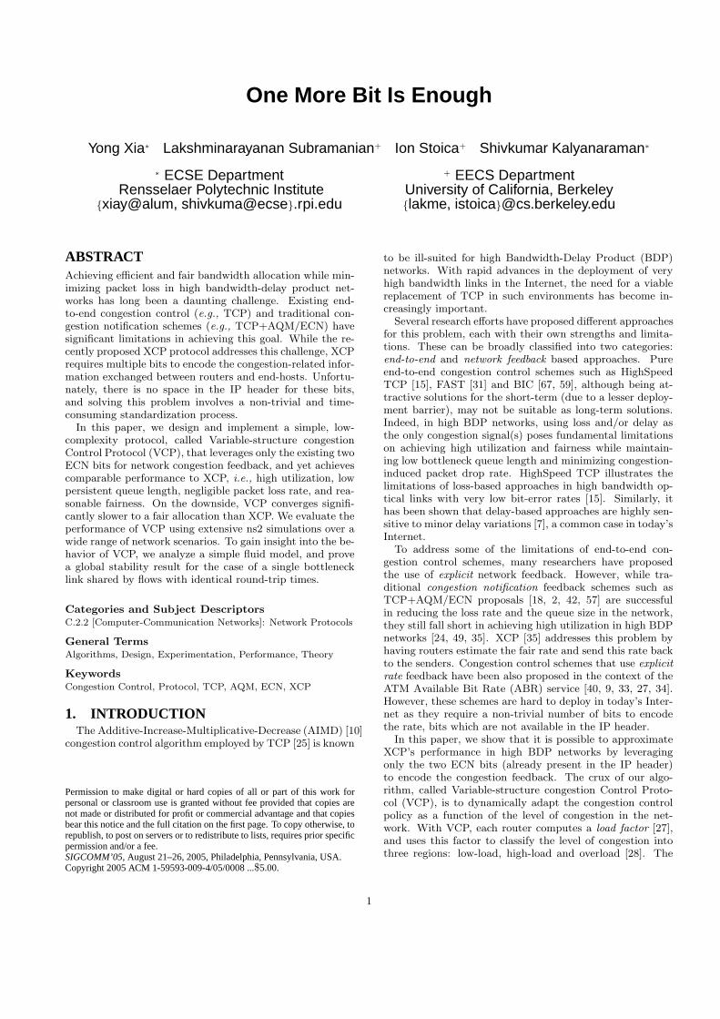
We start our analysis by considering a single bottlenecklink traversed by N flows that have the same RTT, T . Asshown in Figure 11, the load factor ρ(t) received by thesource at a time t is computed based on the sender’s rate attime t− T ,

8

router ρξ

tt−Tsource

destination

time

Figure 11: A simplified VCP model. The source sending

rate at time t − T is used by the router to calculate a

load factor ρ, which is echoed back from the destination

to the source at time t. Then the source adjusts its MI

parameter ξ(ρ(t)) based on the load factor ρ(t).

ρ(t) =

∑Ni=1 wi(t− T )

γCT, (11)

where wi(t) is the flow i’s congestion window at time t, Cis the link capacity, and 0 < γ ≤ 1 is the target link uti-lization. We assume that wi(t) is a positive, continuous anddifferentiable function, and T is a constant.

Since ξ(ρ(t)) is proportional to the available bandwidth,the MIAIMD algorithm tracks the available bandwidth ex-ponentially fast and thus achieves efficiency. It also con-verges to fairness as we will show in Theorem 2. 2

Using (9) to sum over all N flows yields

w(t) =1

T· [ w(t) · ξ(ρ(t)) + Nα ] (12)

where w(t) =∑N

i=1 wi(t) is the sum of all the congestionwindows. This result, together with (10) and (11), leads to

w(t) =1

T· {κ · w(t) · [ γCT

w(t− T )− 1 ] + Nα } (13)

where w(t) > 0. We assume the initial condition w(t) = N(i.e., wi(t) = 1), for all t ∈ [−T, 0]. In [66], we prove thefollowing global stability result.

Theorem 1. Under the model (9), (10) and (11) wherea single bottleneck is shared by a set of synchronous flowswith the same RTT, if κ ≤ 1

2, then the delayed differential

equation (13) is globally asymptotically stable with a uniqueequilibrium w∗ = γCT + N α

κ, and all the flows have the

same steady-state rate r∗i = γCN

+ ακT

.

This result has two implications. First, the sufficient con-dition κ ≤ 1

2holds for any link capacity, any feedback delay,

and any number of flows. Furthermore, the global stabilityresult does not depend on the network parameters. Second,this result is optimal in that at the equilibrium, the systemachieves all the design goals: high utilization, fairness, zerosteady-state queue length, and zero packet loss rate—this isbecause we can always adjust γ such that the system stabi-lizes at a steady-state utilization slightly less than 1.

Importance of γ: While (11) defines γ as the target

utilization, the actual utilization is w∗CT

= γ + ακP

where

P = CTN

is the per-flow BDP. To achieve a certain targetutilization γ∗, γ should be treated as a control variable andset to γ = γ∗ − α

κP. For more details on how to make this

adjustment process automatic without even knowing α, κand P , we refer the reader to [66].

2Theorem 2 actually proves the max-min fairness for a generalmultiple-bottleneck topology. For a single link, max-min fairnessmeans each flow gets an equal share of the link capacity.

Next, we consider a more general multiple-bottleneck net-work topology. Let ρi(t) denote the maximal link load fac-tor on flow i’s path Li that includes a subset of links, i.e.,Li = { l | flow i traverses link l}. The MI parameter of flowi is then

ξ(ρi(t)) = κ · [ 1

ρi(t)− 1 ], (14)

where ρi(t) = maxl∈Li ρl(t), ρl(t) =∑

i∈Ilwi(t−T )

γClT, and the

subset of flows Il = { i | flow i traverses link l}. We provethe following fairness result in [66].

Theorem 2. In a multiple-bottleneck topology where allflows have the same round-trip time T , if there exists aunique equilibrium, then the algorithm defined by (9) and(14) allocates a set of max-min fair rates r∗i = α

κT (1− 1maxl∈Li

ρ∗l

)

where ρ∗l =∑

i∈Ilw∗i

γCT.

To better understand this result note that a flow’s sendingrate is determined by the most congested bottleneck linkon its path. Thus, the flows traversing the most congestedbottleneck links in the system will naturally experience thelowest throughputs.

Having established the stability and fairness properties ofthe MIAIMD model, we now turn our attention on the con-vergence of the VCP protocol. The following two theorems,proved in [66], give the convergence properties.

Theorem 3. The VCP protocol takes O(log C) RTTs toclaim (or release) a major part of any spare (or over-used)capacity C.

Theorem 4. The VCP protocol takes O(P log ∆P ) RTTsto converge onto fairness for any link, where P is the per-flow bandwidth-delay product, and ∆P > 1 is the largestcongestion window difference between flows sharing that link.

Not surprisingly, due to the use of MI in the low-loadregion, VCP converges exponentially fast to high utilization.On the other hand, VCP’s convergence time to fairness issimilar to other AIMD-based protocols, such as TCP+AQM.In contrast, explicit feedback schemes like XCP require onlyO(log ∆P ) RTTs to converge to fairness. This is becausethe end-host based AIMD algorithms improve fairness perAIMD epoch, which includes O(P ) rounds of AI and oneround of MD, while the equivalent operation in XCP takesonly one RTT.

The VCP protocol can be viewed as an approximation ofthe MIAIMD model along three axes. First, the MIAIMDmodel uses the exact load factor feedback, ρ(t), while VCPuses a quantized value of the load factor. Second, in theMI and AI phases, VCP uses either the multiplicative factoror the additive factor term, but not both as the MIAIMDmodel does. Third, in the overload region, VCP applies aconstant MD parameter β instead of ξ(ρ(t)).

The comparison between the simulation results of VCPand the analytical results of the MIAIMD model suggeststhat the two differ most notably in terms of the fairnessmodel. While in the case of multiple bottleneck links, theMIAIMD model achieves max-min fairness [4], VCP tendsto allocate more bandwidth to flows that traverse fewer bot-tleneck links (see Section 4.2). This is because VCP relieson the quantized representation of the load factor instead ofthe exact value.

9

6. DISCUSSIONSSince VCP switches between MI, AI, and MD algorithms

based on the load factor feedback, there are natural concernswith respect to the impact of these switches on the systemstability, efficiency, and fairness, particularly in systems withhighly heterogeneous RTTs. We discuss these concerns inthis section. We discuss VCP’s TCP-friendliness and incre-mental deployment in [66].

6.1 Stability under Heterogeneous DelaysAlthough the MIAIMD model presented in Section 5 is

provably stable, it assumes synchronous feedback. To ac-commodate heterogeneous delays, VCP scales the MI/AIparameters such that flows with different RTTs act as ifthey were having the same RTT. This scaling mechanismis also essential to achieving fair bandwidth allocation, asdiscussed in Section 3.4.

In normal circumstances, VCP makes a transition to MDonly from AI. However, even if VCP switches directly fromMD to MI, if the demand traffic at the router does notchange significantly, VCP will eventually slide back into AI.

Finally, to prevent the system from oscillating betweenMI and MD, we set the load factor transition point ρl to80%, and set the MD parameter β to 0.875 > ρl. This givesus a safety margin of 7.5%.

The extensive simulation results presented in Section 4suggest that VCP is indeed stable over a large variety of net-work scenarios including per-flow bandwidths from 2Kbps to100Mbps and RTTs from 1ms to 1.5s.

6.2 Influences of Mode SlidingFrom an efficiency perspective, VCP’s goal is to bring and

maintain the system into the high utilization region. WhileMI enables VCP to quickly reach the high link utilization,VCP needs also to make sure that the system remains in thisstate. The main mechanisms employed by VCP to achievethis goal is the scaling of the MI/AI parameters for flowswith different RTTs. In addition to improving fairness, thisscaling is essential to avoid oscillations. Otherwise, a flowwith a low RTT may apply MI several times during theestimation interval, tρ, of the link load factor. Other mech-anisms employed by VCP to maintain high efficiency includechoosing an appropriate value of the MD parameter to re-main in the high utilization region, using a safety margin be-tween MI and AI, and bounding the burstiness (Section 4.3).

As discussed in Section 3.4, there are two major concernswith respect to fairness. First, a flow with a small RTTprobes the network faster than a flow with a large RTT.Thus, the former may increase its bandwidth much fasterthan the latter. Second, it will take longer for a large-RTTflow to switch from MI to AI than a small-RTT flow. Thismay give the large-RTT flow an unfair advantage. VCP ad-dresses the first issue by using the RTT scaling mechanism(see (6)-(7)). To address the second issue, VCP bounds theMI gain, as discussed in Section 4.3. To illustrate the effec-tiveness of limiting the MI gain, Figure 12 shows the con-gestion window evolution for two flows with RTTs of 50msand 500ms, respectively, traversing a single 10Mbps link. Attime 12.06s, the 50ms-RTT flow switches from MI to AI. Incontrast, due to its larger RTT, the 500ms-RTT flow keepsperforming MI until time 12.37s. However, because VCPlimits the MI gain of the 500ms-RTT flow, the additional

BA

MD <==> AI

MI ==> AI

0

10

20

30

40

50

60

70

80

0 5 10 15 20

Cong

estion

Wind

ow (p

ackets

)

Time (sec)

flow with rtt = 50msflow with rtt = 500ms

Figure 12: The congestion window dynamics of

two flows with dramatically different RTTs (50ms vs.

500ms). Due to its longer delay, the larger-RTT flow al-

ways slides its mode later than the one with smaller RTT

(see the regions labeled as A and B). However, the ef-

fect of this asynchronous switching is accommodated by

VCP and does not prevent it from maintaining stability

and achieving efficiency and fairness.

bandwidth acquired by this flow during the 0.31s intervalis only marginal when compared to the bandwidth acquiredby the 50ms-RTT flow.

7. RELATED WORKThis paper builds upon a great body of related work, par-

ticularly XCP [35], TCP [25, 1, 17, 51], AIMD [10, 29],AQM [18, 2, 42] and ECN [57, 58]. Congestion control ispioneered by TCP and AIMD. The research on AQM startsfrom RED [18, 47], followed by Blue [14], REM [2], PI con-troller [23], AVQ [21, 42], and CHOKe [54], etc. Below werelate VCP to three categories of congestion control schemesand a set of analytical results.

Explicit rate based schemes: XCP regulates sourcesending rate with decoupled efficiency control and fairnesscontrol and achieves excellent performance. ATM ABR ser-vice (e.g., see [40, 9, 33, 27, 34]) previously proposes explicitrate control. VCP learns from these schemes. In contrast,VCP is primarily an end-host based protocol. This key dif-ference brings new design challenges not faced by XCP (andthe ATM ABR schemes) and thus VCP is not just a “two-bit” version of XCP. The idea of classifying network loadinto different regions is originally presented in [28]. The linkload factor is suggested as a congestion signal in [27], basedon which VCP quantizes and encodes it for a more compactrepresentation for the degree of congestion. MaxNet [65]uses the maximal congestion information among all the bot-tlenecks to achieve max-min fairness. QuickStart [26] oc-casionally uses several bits per packet to quickly ramp upsource sending rates. VCP is complementary to QuickStartas it constantly uses two bits per packet.

Congestion notification based schemes: For high BDPnetworks, according to [35], the performance gap betweenXCP and TCP+RED/REM/AVQ/CSFQ [60] with one-bitECN support seems large. VCP generalizes one-bit ECNand applies some ideas from these AQM schemes. For exam-ple, RED’s queue-averaging idea, REM’s match-rate-clear-buffer idea and AVQ’s virtual-capacity idea obviously findthemselves in VCP’s load factor calculation in Equation (1).This paper demonstrates that the marginal performance gainfrom one-bit to two-bit ECN feedback could be significant.On the end-host side, two-bit ECN is also used to choosedifferent decrease parameters for TCP in [13], which is verydifferent from the way VCP uses. GAIMD [68] and the bino-

10

mial control [3] generalize the AIMD algorithm, while VCPgoes even further to combine MIMD with AIMD.

Pure end-to-end schemes: Recently there have beenmany studies on the end-to-end congestion control for highBDP networks. HighSpeed TCP [15] extends the standardTCP by adaptively setting the increase/decrease parame-ters according to the congestion window size. H-TCP [45]employs an adaptive AIMD with its parameters set as func-tions of the elapsed time since the last congestion event.Adaptive TCP [38] also applies dynamic AIMD parameterswith respect to the changing network conditions. STCP [36]changes to a fixed MIMD algorithm. FAST [31] uses queue-ing delay, like TCP Vegas [6], instead of packet loss, asits primary congestion signal and improves Vegas’ Additive-Increase-Additive-Decrease policy with a proportional con-troller. BIC [67, 59] adds a binary search phase into thestandard TCP to probe the available bandwidth in a log-arithmic manner. LTCP [5] layers congestion control oftwo scales for high speed, large RTT networks. TCP West-wood [8] enhances the loss-based congestion detector usingmore robust bandwidth estimation techniques. All theseend-to-end schemes do not need explicit feedback. There-fore, it is hard for them to achieve both low persistent bottle-neck queue length and almost zero congestion-caused packetloss rate. VCP does need explicit two-bit ECN but is able tomaintain low queue and almost zero loss. However, it is un-clear whether these end-to-end schemes, if given AQM/ECNsupport from network, can achieve similar performance asVCP in high BDP networks.

Analytical Results: The nonlinear optimization frame-work [37, 48, 41] provides the above schemes a unified the-oretic underpin and proposes a class of control algorithms.The local stability of the algorithms when homogeneous de-lay is present is considered by [32, 62] and then extended tothe case of heterogeneous delays by [50]. The local stabilityof a modified algorithm for the case of heterogeneous delaysis proved by [70], which establishes a model that is similarto what we show in Section 5. In contrast, a global stabil-ity result is obtained in this paper for the case of a singlebottleneck with homogeneous delays. The global stability ofmore general congestion controllers are considered by otherresearchers, e.g., in [63, 12, 69].

Variable-structure control with sliding modes has a longhistory in control theory [61]. It is useful when a set offeatures are desired in a system but no single algorithm canprovide all of them. In computer networking areas, it hasbeen used to solve a traffic engineering problem in [43]. Ourwork can be viewed as an application of this idea to networkcongestion control.

8. SUMMARYIn this paper, we propose VCP, a simple, low-complexity

congestion control protocol for high BDP networks. Us-ing extensive ns2 simulations, we show that VCP achieveshigh utilization, reasonable fairness, low persistent bottle-neck queue, and negligible packet loss rate. VCP achievesall these desirable properties while requiring only two bitsto encode the network congestion information. Since it canleverage the two ECN bits to carry this information, VCPrequires no changes of the IP header. In this respect, VCPcan be seen as an extension of the TCP+AQM/ECN pro-posals that scales to high BDP networks.

To better understand the behavior of VCP, we proposea fluid model, and use this model to analyze the efficiency,fairness, and convergence properties of a simplified version ofVCP. Particularly, we prove that the model is globally stablefor the case of a single bottleneck link shared by long-livedflows with identical RTTs.

As future work, it would be interesting to study what im-provements are possible in VCP by using more than twobits for the congestion-related information. One obviouspossibility would be to use a finer granularity encoding ofthe network load factor to improve the fairness convergencespeed. While in this paper we evaluate VCP through exten-sive simulations, ultimately, only a real implementation anddeployment will allow us to asses the strengths and limita-tions of VCP.

9. ACKNOWLEDGEMENTSThe authors are very grateful to Sally Floyd, Dina Katabi,

K. K. Ramakrishnan, Scott Shenker and the anonymous re-viewers for their insightful comments, and to Dina Katabifor shepherding this paper. The authors owe their gratitudeto Jianghai Hu and John Wen for proof-reading Theorem 1,to Xinzhe Fan and Yang Kuang for their suggestions on thestability analysis, to Dilip Anthony Joseph and Jayanthku-mar Kannan for reading earlier drafts of this paper, to DavidHarrison for making his ns2 graphing tools available, and toLan Shi for her help. We would like to thank them all.

10. REFERENCES

[1] M. Allman, V. Paxson, and W. Stevens. TCP CongestionControl. IETF RFC 2581, April 1999.

[2] S. Athuraliya, V. Li, S. Low, and Q. Yin. REM: Active QueueManagement. IEEE Network, 15(3):48-53, May 2001.

[3] D. Bansal and H. Balakrishnan. Binomial Congestion ControlAlgorithms. INFOCOM’01, April 2001.

[4] D. Bertsekas and R. Gallager. Data Networks. 2nd Ed., Simon& Schuster, December 1991.

[5] S. Bhandarkar, S. Jain, and A. Reddy. Improving TCPPerformance in High Bandwidth High RTT Links UsingLayered Congestion Control. PFLDNet’05, February 2005.

[6] L. Brakmo and L. Peterson. TCP Vegas: End to EndCongestion Avoidance on a Global Internet. IEEE J. SelectedAreas in Communications, 13(8):1465-1480, October 1995.

[7] H. Bullot and R. Les Cottrell. Evaluation of Advanced TCPStacks on Fast Long-Distance Production Networks. Availableat http://www.slac.stanford.edu/grp/scs/net/talk03/tcp-slac-nov03.pdf.

[8] C. Casetti, M. Gerla, S. Mascolo, M. Sansadidi, and R. Wang.TCP Westwood: End-to-End Congestion Control forWired/Wireless Networks. Wireless Networks Journal,8(5):467-479, September 2002.

[9] A. Charny, D. Clark, and R. Jain. Congestion Control withExplicit Rate Indication. IEEE ICC’95, June 1995.

[10] D. Chiu and R. Jain. Analysis of the Increase/DecreaseAlgorithms for Congestion Avoidance in Computer Networks.J. of Computer Networks and ISDN, 17(1):1-14, June 1989.

[11] M. Crovella and A. Bestavros. Self-Similarity in World WideWeb Traffic: Evidence and Possible Causes. IEEE/ACMTrans. Networking, 5(6):835-846, December 1997.

[12] S. Deb and R. Srikant. Global Stability of CongestionControllers for the Internet. IEEE Trans. Automatic Control,48(6):1055-1060, June 2003.

[13] A. Durresi, M. Sridharan, C. Liu, M. Goyal, and R. Jain.Multilevel Explicit Congestion Notification. SCI’01, July 2001.

[14] W. Feng, K. Shin, D. Kandlur, and D. Saha. The BLUE activequeue management algorithms. IEEE/ACM Trans.Networking, 10(4):513-528, August 2002.

[15] S. Floyd. HighSpeed TCP for Large Congestion Windows.IETF RFC 3649, December 2003.

11

[16] S. Floyd, M. Handley, J. Padhye, and J. Widmer.Equation-Based Congestion Control for Unicast Applications.SIGCOMM’00, August 2000.

[17] S. Floyd and T. Henderson. The NewReno Modification toTCP’s Fast Recovery Algorithm. IETF RFC 2582, April 1999.

[18] S. Floyd and V. Jacobson. Random Early Detection Gatewaysfor Congestion Avoidance. IEEE/ACM Trans. Networking,1(4):397-413, August 1993.

[19] S. Floyd and V. Paxson. Difficulties in Simulating the Internet.IEEE/ACM Trans. Networking, 9(4):392-403, August 2001.

[20] E. Gafni and D. Bertsekas. Dynamic Control of Session InputRates in Communication Networks. IEEE Trans. AutomaticControl, 29(11):1009-1016, November 1984.

[21] R. Gibbens and F. Kelly. Resource Pricing and the Evolutionof Congestion Control. Automatica, 35:1969-1985, 1999.

[22] K. Gopalsamy. Stability and Oscillations in Delay DifferentialEquations of Population Dynamics. Kluwer AcademicPublishers, 1992.

[23] C. Hollot, V. Misra, D. Towlsey, and W. Gong. On DesigningImproved Controllers for AQM Routers Supporting TCPFlows. INFOCOM’01, April 2001.

[24] C. Hollot, V. Misra, D. Towsley, and W. Gong. Analysis andDesign of Controllers for AQM Routers Supporting TCP Flows.IEEE Trans. Automatic Control, 47(6):945-959, June 2002.

[25] V. Jacobson. Congestion Avoidance and Control.SIGCOMM’88, August 1988.

[26] A. Jain and S. Floyd. Quick-Start for TCP and IP. IETFInternet Draft draft-amit-quick-start-02.txt, October 2002.

[27] R. Jain, S. Kalyanaraman, and R. Viswanathan. The OSUScheme for Congestion Avoidance in ATM Networks: LessonsLearnt and Extensions. Performance Evaluation, 31(1):67-88,November 1997.

[28] R. Jain and K. K. Ramakrishnan. Congestion Avoidance inComputer Networks with A Connectionless Network Layer:Concepts, Goals, and Methodology. Proc. IEEE ComputerNetworking Symposium, April 1988.

[29] R. Jain, K. K. Ramakrishnan, and D. Chiu. CongestionAvoidance in Computer Networks with a ConnectionlessNetwork Layer. DEC-TR-506, August 1987.

[30] H. Jiang and C. Dovrolis. Passive Estimation of TCPRound-Trip Times. ACM Computer Communications Review,32(3):75-88, July 2002.

[31] C. Jin, D. Wei, and S. Low. FAST TCP: Motivation, Architec-ture, Algorithms, Performance. INFOCOM’04, March 2004.

[32] R. Johari and D. Tan. End-to-End Congestion Control for theInternet: Delays and Stability. IEEE/ACM Trans.Networking, 9(6):818-832, December 2001.

[33] L. Kalampoukas, A. Varma, and K. K. Ramakrishnan.Dynamics of an Explicit Rate Allocation Algorithm forAvailable Bit-Rate (ABR) Service in ATM Networks.Proceedings of the IFIP/IEEE Conference on BroadbandCommunications, April 1996.

[34] S. Kalyanaraman, R. Jain, S. Fahmy, R. Goyal, and B.Vandalore. The ERICA Switch Algorithm for ABR TrafficManagement in ATM Networks. IEEE/ACM Trans.Networking, 8(1), February 2000.

[35] D. Katabi, M. Handley, and C. Rohrs. Congestion Control forHigh Bandwidth-Delay Product Networks. SIGCOMM’02,August 2002.

[36] T. Kelly. Scalable TCP: Improving Performance in HighspeedWide Area Networks. Submitted, December 2002.

[37] F. Kelly, A. Maulloo, and D. Tan. Rate Control inCommunication Networks: Shadow Prices, ProportionalFairness and Stability. Journal of the Operational ResearchSociety, 49:237-252, 1998.

[38] A. Kesselman and Y. Mansour. Adaptive TCP Flow Control.PODC’03, July 2003.

[39] Y. Kuang. Delay Differential Equations with Applications inPopulation Dynamics. Academic Press, 1993.

[40] H. Kung, T. Blackwell, and A. Chapman. Credit-Based FlowControl for ATM Networks: Credit Update Protocol, AdaptiveCredit Allocation, and Statistical Multiplexing.SIGCOMM’94, August 1994.

[41] S. Kunniyur and R. Srikant. End-To-End Congestion Control:Utility Functions, Random Losses and ECN Marks.INFOCOM’00, March 2000.

[42] S. Kunniyur and R. Srikant. Analysis and Design of anAdaptive Virtual Queue (AVQ) Algorithm for Active QueueManagement. SIGCOMM’01, August 2001.

[43] C. Lagoa, H. Che and B. Movsichoff. Adaptive ControlAlgorithms for Decentralized Optimal Traffic Engineering inthe Internet. IEEE/ACM Trans. Networking, 12(3):415-428,June 2004.

[44] T. Lakshman and U. Madhow. The Performance of TCP/IPfor Networks with High Bandwidth-delay Products andRandom Loss. IEEE/ACM Trans. Networking, 5(3):336-350,June 1997.

[45] D. Leith and R. Shorten. H-TCP: TCP for High-speed andLong-distance Networks. PFLDnet’04, February 2004.

[46] W. Leland, M. Taqqu, W. Willinger, and D. Wilson. On theSelf-Similar Nature of Ethernet Traffic. SIGCOMM’93, August1993.

[47] D. Lin and R. Morris. Dynamics of Random Early Detection.SIGCOMM’97, August 1997.

[48] S. Low and D. Lapsley. Optimization Flow Control, I: BasicAlgorithm and Convergence. IEEE/ACM Trans. Networking,7(6):861-875, December 1999.

[49] S. Low, F. Paganini, J. Wang, and J. Doyle. Linear Stability ofTCP/RED and a Scalable Control. Computer NetworksJournal, 43(5):633-647, December 2003.

[50] L. Massoule. Stability of Distributed Congestion Control withHeterogeneous Feedback Delays. IEEE Trans. AutomaticControl, 47(6):895-902, June 2002.

[51] M. Mathis, J. Mahdavi, S. Floyd, and A. Romanow. TCPSelective Acknowledgement Options. IETF RFC 2018,October 1996.

[52] Network Simulator ns-2. Http://www.isi.edu/nsnam/ns/.

[53] J. Padhye, V. Firoiu, D. Towsley, and J. Kurose. ModelingTCP Throughput: A Simple Model and its EmpiricalValidation. SIGCOMM’98, September 1998.

[54] R. Pan, K. Psounis, and B. Prabhakar. CHOKe, A StatelessActive Queue Management Scheme for Approximating FairBandwidth Allocation. INFOCOM’00, March 2000.

[55] V. Paxson. End-to-End Internet Packet Dynamics.SIGCOMM’97, September 1997.

[56] V. Paxson and S. Flyod. Wide-Area Traffic: The Failure ofPoisson Modeling. SIGCOMM’94, August 1994.

[57] K. K. Ramakrishnan and S. Floyd. The Addition of ExplicitCongestion Notification (ECN) to IP. IETF RFC 3168,September 2001.

[58] K. K. Ramakrishnan and R. Jain. A Binary Feedback Schemefor Congestion Avoidance in Computer Networks.SIGCOMM’88, August 1988.

[59] I. Rhee and L. Xu. CUBIC: A New TCP-Friendly High-SpeedTCP Variant. PFLDNet’05, February 2005.

[60] I. Stoica, S. Shenker, and H. Zhang. Core-Stateless FairQueueing: Achieving Approximately Fair BandwidthAllocations in High Speed Networks. SIGCOMM’98,September 1998.

[61] V. Utkin. Variable Structure Systems with Sliding Modes.IEEE Trans. Automatic Control, 22(2):212-222, April 1977.

[62] G. Vinnicombe. On the Stability of End-to-end CongestionControl for the Internet. Univ. of Cambridge Tech ReportCUED/F-INFENG/TR.398, December 2000.

[63] J. Wen and M. Arcak. A Unifying Passivity Framework forNetwork Flow Control. INFOCOM’03, March 2003.

[64] E. Wright. A Non-linear Difference-Differential Equation. J.Reine Angew. Math., 494:66-87, 1955.

[65] B. Wydrowski and M. Zukerman. MaxNet: A CongestionControl Architecture for Maxmin Fairness. IEEE Comm.Letters, 6(11):512-514, November 2002.

[66] Y. Xia, L. Subramanian, I. Stoica, and S. Kalyanaraman. OneMore Bit is Enough. UC Berkeley Tech Report, June 2005.

[67] L. Xu, K. Harfoush, and I. Rhee. Binary Increase CongestionControl (BIC) for Fast Long-Distance Networks.INFOCOM’04, March 2004.

[68] Y. Yang and S. Lam. General AIMD Congestion Control.ICNP’00, November 2000.

[69] L. Ying, G. Dullerud, and R. Srikant. Global Stability ofInternet Congestion Controllers with Heterogeneous Delays.Proc. American Control Conference, June 2004.

[70] Y. Zhang, S. Kang, and D. Loguinov. Delayed Stability andPerformance of Distributed Congestion Control.SIGCOMM’04, September 2004.

12

11. APPENDIX

11.1 Proof of Theorem 1To analyze the stability of Equation (13), let y(t) = γCT

w(t),

then after some manipulation we obtain

y(t) = k1 y(t) [1− y(t− T )− k2 y(t)] (15)

where k1 = κT

> 0, and k2 = Nακ γCT

> 0. We also have, for

all t > 0, y(t) ≥ 0 since w(t) > 0, and the initial conditiony(t) > 0 (since we assume w(t) = N < ∞) for t ∈ [−T, 0].

Observing that the trivial solution y(t) = 0 is not a stableequilibrium of this equation, since any small perturbationwill move the system further off the origin, we thereforeassume y(t) > 0, ∀t > 0. Physically, this assumption meansthat, at any time, the congestion window w(t) is not infinite,which generally holds in reality.

To prove this theorem, we first establish two lemmas, ap-plying the techniques developed in [64, 39, 22], to which wewould like to give credit.

Lemma 1. If κ ≤ 1 − NαγCT

, then (15) has a unique equi-

librium y∗ = 11+k2

that is globally asymptotically stable.

Proof. Substituting x(t) = y(t)− y∗ in (15) we get

x(t) = −k1 [ y∗ + x(t) ] [ x(t− T ) + k2 x(t) ] (16)

with a solution

y∗+ x(t) = [ y∗+ x(t0) ] · e−k1∫ t−T

t0−T[ x(τ)+k2 x(τ+T ) ] dτ

(17)

where t0 is a constant [39]. To show limt→+∞ x(t) = 0, wetreat separately the following two cases.

Case #1. If x(t) is not oscillatory, i.e., |x(t)| > 0 when t >t1 for some t1 > 0. For x(t) > 0, when t > t1 + T , we havex(t) < 0 due to (15), which means x(t) is strictly decreasingfor all t > t1 + T . Because x(t) > 0, there exists a constantc such that limt→+∞ x(t) = c and thus limt→+∞ x(t) = 0.We must have c = 0. Otherwise c > 0, then limt→+∞ x(t) =−c k1(y

∗ + c)(1 + k2) < 0 according to (15), resulting in acontradiction. The same analysis applies to when x(t) < 0;

Case #2. If x(t) is oscillatory, i.e., there is a sequencet′l > t2 for some t2 > 0, t′l → +∞ as l → +∞, such thatx(t′l) = 0 for all t′l. We firstly prove that x(t) is boundedwhen t > t2. Obviously x(t) is lower bounded, since x(t) =y(t)− y∗ > −y∗ as y(t) > 0. Now we show that x(t) is alsoupper bounded. Let t3, t4 ∈ (t2,∞), t3 < t4 be any twoconsecutive zeros of x(t) such that x(t) > 0 for t3 < t < t4.( If x(t) < 0 we get an upper bound 0.) Because w(t) iscontinuous and differentiable, so does x(t) = y(t) − y∗ =γCTw(t)

−y∗. Since x(t3) = x(t4) = 0, x(t) has a local maximum

in the interval (t3, t4). Denote it as x(tm) where t3 < tm <t4, we have x(t) ≤ x(tm) for all t ∈ (t3, t4). We also havex(tm) = 0, which deduces x(tm − T ) + k2 x(tm) = 0 from(16). Substituting this result, x(t) > −y∗, and y∗ = 1

1+k2

in (17) and setting t0 = tm − T , t = tm, we get

−k1

∫ t−T

t0−T

[ x(τ) + k2 x(τ + T ) ] dτ < k1T

and thus

x(t) ≤ x(tm) <y∗(ek1T − 1)

1 + k2ek1T(18)

for all t ∈ [t3, t4]. Repeating this process for all the consec-utive zero pairs of x(t) in (t2,∞), we conclude that x(t) isbounded for t > t2.

Since x(t) is continuous and bounded, denote

u = lim supt→+∞

x(t), v = − lim inft→+∞

x(t). (19)

Obviously we have

u ≥ −v. (20)

We now prove that u = v = 0 (therefore limt→+∞ x(t) = 0).Let ε > 0 be an arbitrarily small constant such that, for allt > t5 = t5(ε) > 0,

−v − ε < x(t) < u + ε. (21)

As per the definition of u, we can always find a local max-imum x(tn) > u − ε for tn > t5 + T . Applying the sametechnique used to derive (18) on tn, plus the left half of(21), we get

u− ε < x(tn) <y∗[ eφ(v+ε) − 1 ]

1 + k2eφ(v+ε)(22)

where φ = k1(1 + k2)T = κ + NαγCT

> 0. Since (22) holds forall ε > 0, we conclude

u ≤ y∗(eφv − 1)

1 + k2eφv, (23)

where 0 < y∗ = 11+k2

< 1 and k2 > 0. Following similar

steps in deriving (23) on a local minimum generates

v ≤ y∗(1− e−φu)

1 + k2e−φu. (24)

Now we discuss the following combinations of u and v andshow that the only possibility is u = v = 0, if φ ≤ 1.

i) If u < 0, then v < 0 according to (24), so −v > 0 > u,violating (20);

ii) If u = 0, then v ≥ 0 from (20). We have v ≤ 0 as welldue to (24). Therefore v = 0;

iii) If u > 0, then v > 0 according to (23). From (24) wehave v < y∗ < 1. If φ ≤ 1, we get

1 + u < eφv ≤ ev < e1−e−φu ≤ e1−e−u

. (25)

However, for u > 0, we have

1 + u− e1−e−u

=

∫ u

0

∫ ζ

0

(1− e−η)e(1−e−η−η)dηdζ > 0

which is a conflict with (25).To sum up, we must have u = v = 0 if φ ≤ 1, i.e.,

κ ≤ 1− NαγCT

, which deduces limt→+∞ x(t) = 0.

Next we turn to the second lemma.

Lemma 2. If κ < NαγCT

, then (15) has a unique equilibrium

y∗ = 11+k2

that is globally asymptotically stable.

Proof. Consider the following function [22]

V (t) = y(t)− y∗ log y(t) +k1

2

∫ t

t−T

[ y(τ)− y∗]2 dτ. (26)

13

Again let x(t) = y(t)− y∗. Due to (15) and k1 > 0 we have

dV

dt= y(t) [1− y∗

y(t)] +

k1

2[ x2(t)− x2(t− T ) ]

=y(t) x(t)

y(t)+

k1

2[ x2(t)− x2(t− T ) ]

= −k1 x(t)[k2 x(t) + x(t− T )] +k1

2[ x2(t)− x2(t− T ) ]

= −k1

2[ (2k2 − 1) x2(t) + x2(t− T ) + 2x(t)x(t− T ) ]

= −k1

2{ 2(k2 − 1) x2(t) + [x(t) + x(t− T )]2 }

≤ −k1(k2 − 1) x2(t). (27)

Integrating this inequality over [0, t], we have

V (t) + k1(k2 − 1)

∫ t

0

x2(τ) dτ ≤ V (0) (28)

where V (0) = y(0) − y∗ log y(0) + k12

∫ 0

−T[ y(τ) − y∗]2 dτ is

bounded since y(t) is finite when t ∈ [−T, 0].Note we have proved in Lemma 1 that x(t) is bounded for

all t > t2 for some t2 > 0. So does y(t) because y(t) = x(t)+y∗. Thus V (t) is also bounded. If k2 > 1 (i.e., κ < Nα

γCT),

we must have limt→+∞ x(t) = 0 since otherwise we obtain

k1(k2 − 1)∫ t

0x2(τ) dτ → +∞ as t → +∞, resulting in a

conflict with (28).

Now we are ready to prove the theorem. When κ ≤ 12, we

always have at least one of the two inequalities, κ ≤ 1− NαγCT

and κ < NαγCT

, holds. We thus complete the proof using

the above two lemmas. The equilibrium of (13) is thereforew∗ = γCT

y∗ = γCT + N ακ.

The steady-state load factor, due to (11), is ρ∗ = w∗γCT

=

1 + NακγCT

. Let (9) be 0, we obtain, for all i ∈ [1, N ], flow i’s

steady-state congestion window w∗i = γCTN

+ ακ. Its steady-

state rate is thus r∗i =w∗iT

= γCN

+ ακT

. QED.

11.2 Proof of Theorem 2Denote the aggregate rate at link l as Al =

∑i∈Il

ri where

ri = wiT

is the sending rate of flow i. The load factor, ac-

cording to (11), is thus ρl = AlγCl

where Cl is link l’s capacity.

Define function [20]

g(ρl) =α

κT (1− 1ρl

)(29)

which is strictly decreasing when ρl > 1. (Note ρl > 1 for alll ∈ L according to Theorem 1.) Then, if we set w(t) = 0 in(9) and consider (14), we have the equilibrium rate of flowi as

ri =α

κT (1− 1maxl∈Li

ρl)

= minl∈Li

g(ρl)

≤ g(ρl) ∀l ∈ Li. (30)

Consider the subset of link(s) L∗m that has the highestload factor ρ∗m = maxl∈L ρl among all the links:

L∗m = { l ∈ L | ρl = ρ∗m }, (31)

and the subset I∗m of flow(s) that traverse at least one linkin L∗m, i.e.,

I∗m = { i ∈ I |Li ∩ L∗m 6= φ }. (32)

So all the flows in I∗m have the same rate r∗m = g(ρ∗m) =minl∈L g(ρl), which is the lowest rate allocation.

Suppose r∗m is not maximized, then there exists ri1 > r∗mfor i1 ∈ I∗m. If we pick one link l1 from Li1 ∩ L∗m 6= φ,we have ρl1 =

∑i∈Il1

ri/Cl >∑

i∈Il1r∗m/Cl = ρ∗m. How-

ever, because g(ρl) is strictly decreasing, this leads to ri1 ≤g(ρl1) < g(ρ∗m) = r∗m, resulting in a conflict.

If there is no such ri1 > r∗m for i1 ∈ I∗m, we remove the setsL∗m and I∗m from the network and reduce the capacity of theremaining links (if any, otherwise we are done) by the sum ofthe passing flows’ sending rates, then repeat the above pro-cess until there is no link/flow left. The flow rates defined by(30) thus solve a hierarchy of optimization problems withineach of them the minimal allocation is maximized—this isthe definition of max-min fairness. QED.

11.3 Proof of Theorem 3We first consider the MI part of VCP in Section 3.3 when

there is bandwidth to claim. Due to the MI/AI parameterscaling in Section 3.4 that handles RTT difference, we canassume that flows have the same RTT. Suppose the flowsstart from the unit aggregate rate r(0) = 1. At the end ofm rounds of MI, the aggregate rate

r(m) = r(0) · (1 + ξ)m

where ξ = 0.0625 as set in Section 3.3. Given any capacityC > 1, to reach a major part (i.e., the load factor transitionpoint, ρl = 80%) of it with MI, let r(m) = ρ0C, and thenwe obtain

m =log ρlC

log(1 + ξ)= O(log C). (33)

The same result also holds when the flows have to releasebandwidth with the MD algorithm of VCP. Now supposethe initial aggregate rate r(0) = C > 1, to reach r(m) = 1where r(m) = β · r(m− 1) = ... = βm · r(0), we get

m =log C

log(1/β)= O(log C) (34)

as well. QED.

11.4 Proof of Theorem 4For fairness convergence speed we focus on the AIMD part

of VCP in Section 3.3. Consider any bottleneck of capacityC shared by N flows of the same RTT value T . After anMD that cuts the aggregate congestion window w from CT

to βCT , it takes (1−β)CTNα

rounds of AI (which we call anepoch) to increase w from βCT to CT . Note during AI allflows grow the same amount of congestion window; only MDreduces the congestion window difference. For any two flowsi and j, at the m-th epoch, we have

∆wij(m) = β ·∆wij(m− 1) = ... = βm ·∆wij(0),

where ∆wij(m) = wi(m)−wj(m). To reach a small-enoughcongestion window difference, e.g., ∆wij(m) = 1, then wehave

m =log ∆wij(0)

log(1/β).

14

The total number of RTTs spent is

m · (1− β)CT

Nα=

1− β

α log(1/β)· P log ∆wij(0) (35)

where P = CTN

is the per-flow BDP.The fairness convergence time of a link l is obviously the

time needed for the two passing flows with the largest initialcongestion window difference to reach the fair allocation,which is O(P log ∆P ), where ∆P = maxi,j∈Il ∆wij(0).

In contrast, XCP’s fairness convergence time is O(log ∆P ),since it shuffles bandwidth in each round of AIMD control.QED.

15