one-dimensional transient dynamic response of functionally

One-Dimensional Transient Dynamic Response ofFunctionally Graded Spherical Multilayered Media

Ibrahim Abu-Alshaikh and Mehmet Emir KoksalDepartment of Mathematics, Fatih University,

Istanbul 34500, Turkey,Tel.: +90-212-8890810; Fax +90-212-8890832,

E-Mail: [email protected]

5—10 July 2004, Antalya, Turkey – Dynamical Systems and Applications,Proceedings, pp. 1—20

AbstractIn this study, one-dimensional transient dynamic response of functionally

graded spherical multilayered media is investigated. The multilayered mediumconsists of N different layers of functionally graded materials (FGMs), i.e., itis assumed that the stiffness and the density of each layer vary continuouslyin the radial direction, but isotropic and homogeneous in the other two direc-tions. The inner surface of the layered composite is assumed to be subjectedto uniform time-dependent normal stresses; whereas, the outer surface of thecomposite body is assumed free of surface traction or fixed. Furthermore, thecomposite body is assumed to be initially at rest and the layers of the multilay-ered medium are assumed to be perfectly bonded to each other. The method ofcharacteristics is employed to obtain the solutions of this initial-boundary valueproblem. The numerical results are obtained and displayed in curves denotingthe variations of normal stresses with time at different locations. These curvesclearly reveal the scattering effects caused by the reflections and refractions ofwaves at the boundaries and interfaces. The curves also display the effects ofgeometric dispersions and the effects of non-homogeneity in the wave profiles.Furthermore, they properly predict the sharp variations in the field variablesin the neighborhood of the wave fronts. By suitably adjusting the materialconstants the results for the special case of isotropic, homogenous and linearlyelastic multilayered media are obtained and compared with the available solu-tions in the literature and very good agreement is found. Moreover, solutionsfor the case of different FGM layers are also obtained.

Key words: Transient dynamic response, Functionally graded materials,Method of characteristics, Spherical layered media.

1 Introduction

Functionally graded materials (FGMs) are ideal candidates of engineering materialsfor applications involving severe thermal gradients, ranging from thermal structures

1

2 I. Abu-Alshaikh and M. E. Koksal

in advanced aircraft and aerospace engines to microelectronics. These materialsare continuously or discretely changing their thermal and mechanical properties atthe macroscopic or continuum scale. The idea of grading the thermomechanicalproperties of particulate composites was first conceived by a group of materialscientists in Japan (see Refs. [1, 2], for example) who coined the term FGMs todescribe this generation of composite materials. Several models of FGMs have beenconsidered for the case where a dynamic load is applied to the outer boundaries of acomposite body [3]. Largely two models may be used to deal with transient dynamicresponse in the inhomogeneous FGM bodies; they are the homogeneous layeredmodel and the inhomogeneous continuous model. In the first type, the FGM layer issubdivided into a large number of homogeneous thin layers each of which has its ownconstant volume fraction [4]. In the second kind, the FGM plate is subdivided intoinhomogeneous layers whose material properties vary continuously in the directionperpendicular to the layering [5, 6]. Ohyoshi [5, 6] has developed an analyticalmethod using linearly inhomogeneous layer elements approach to investigate wavesthrough inhomogeneous structures.

Due to the fact that, the material properties of inhomogeneous FGMs are func-tions of one or more space variable, wave propagation problems related to FGMsare generally difficult to analyze without employing some numerical approaches.Numerical solutions of one-dimensional stress wave propagation in an FGM platesubjected to shear or normal tractions are discussed by Liu et al. [7, 8], by Han etal. [9] and by Chiu and Erdogan [10]. In these studies, the material properties areassumed to vary in the thickness direction and the FGM plate is divided into homo-geneous layers [7], linearly inhomogeneous elements [8] or quadratic inhomogeneouslayer elements [9]. In [10], the material properties of the FGM plate throughoutthe thickness direction are assumed to be functions with arbitrary powers. Two-dimensional wave propagation in an FGM plate is, recently, discussed applying acomposite wave-propagation model in [11] and using finite element method in [12]to simulate elastic wave propagation in continuously non-homogenous materials.However, to the authors’ best knowledge, the transient dynamic response of a sin-gle or a multilayered spherical FGM body subjected to a uniform pressure wavelethas not been investigated in literature.

In this paper, the method of characteristics is employed to obtain the solutions.This method has been employed effectively in investigating one and two-dimensionaltransient wave propagation problems in multilayered plane, cylindrical and spher-ical layered media [13]—[15]. In these references, the multilayered medium consistsof N layers of isotropic, homogeneous and linearly elastic or viscoelastic mater-ial with one or two relaxation times. A brief review on combining the methodof characteristics with Fourier transform to investigate two-dimensional transientwave propagation in viscoelastic layered media can be found in Abu-Alshaikh et

One-dimensional transient dynamic response 3

al. [16, 17]. It is well known that, for one-dimensional homogeneous case the char-acteristic manifold consists of straight lines in the (r − t) plane (here, t: time; r:space variable) and the canonical equations holding on them are ordinary differen-tial equations which can be integrated accurately using a numerical method, suchas, implicit trapezoidal rule formula [13]—[17]. However, for the inhomogeneousFGM case, the characteristic manifold consists of nonlinear curves in the (r − t)plane and the canonical equations can be integrated approximately along the char-acteristic lines by employing a small time discretization. This numerical techniqueis capable of describing the sharp variation of disturbance in the neighborhood ofthe wave front without showing any sign of instability or noise. Hence, it can beused conveniently for one-dimensional transient wave propagation through FGMs,or it can be combined with a transformation technique to handle two-dimensionaltransient wave propagation through FGMs.

2 Formulation of the problem

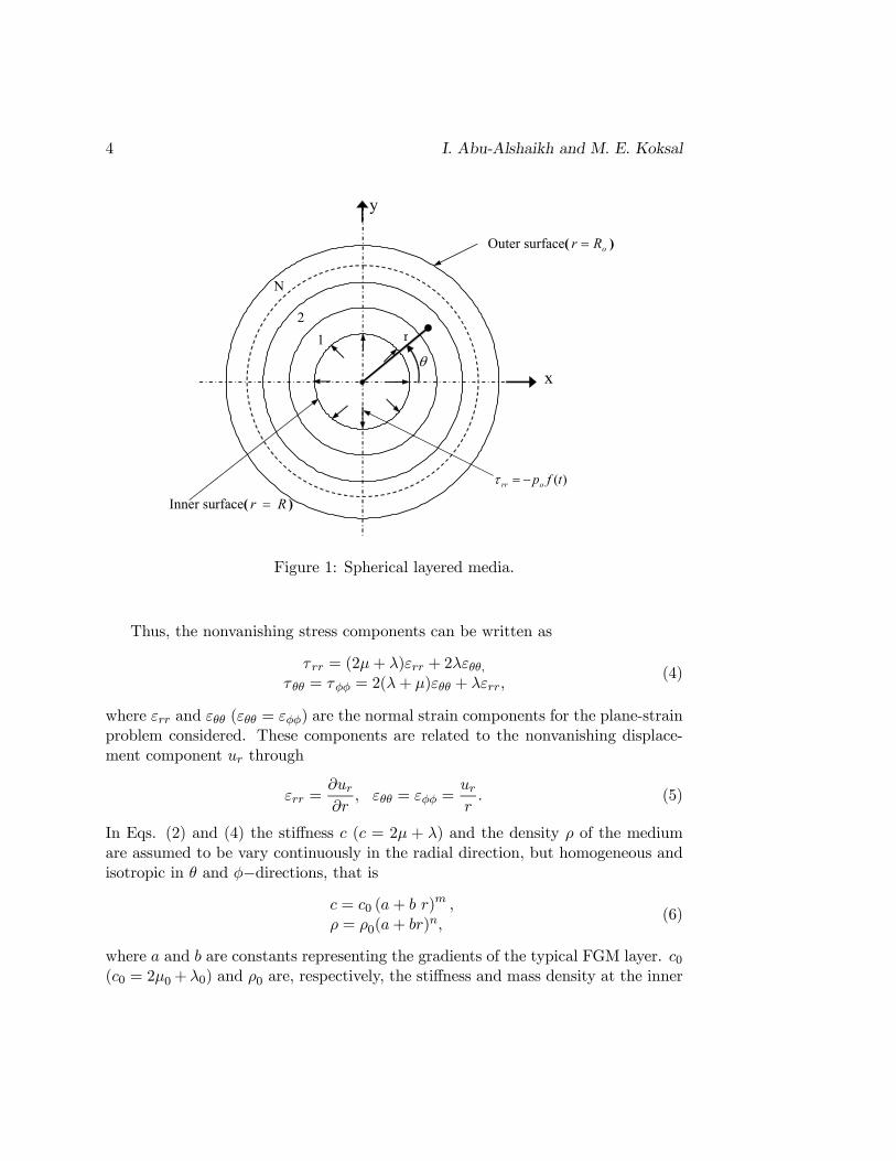
The spherical multilayered medium which is of finite thickness in r−direction con-sists of N different layers, see Fig. 1. It is referred to a spherical coordinate system(r, θ, φ), in which θ and φ are the angles measured from the positive x- and z-axes,respectively. The material properties in each layer are assumed to be vary contin-uously in the r−direction, but isotropic and homogeneous in θ and φ−directions.The inner surface of the layered medium is assumed to be subjected to a uniformtime-dependent pressure wavelet. The outer surface is assumed to be either free ofsurface traction or fixed, or is subject to surface traction similar to that applied atthe inner surface, see Fig. 1. Thus, the problem is a one-dimensional wave propa-gation problem with displacement components uθ and uφ vanishing identically andthe displacement component in the r−direction being a function of r and t, i.e.,

ur = ur(r, t),uθ = uφ = 0.

(1)

Thus, the stress equation of motion for a typical layer can be written, in the absenceof body forces, as

∂τ rr∂r

+2(τ rr − τ θθ)

r= ρ

∂vr∂t

, (2)

where τ rr and τ θθ are the normal stress components in r and θ−directions, respec-tively, ρ is the mass density of the typical layer considered and vr is the componentof the particle velocity in the r−direction, i. e.,

vr =∂ur∂t

. (3)


Outer surface( oRr = )

12

N

θ

)(tfporr −=τ

Inner surface( Rr = )

r

x

y

Figure 1: Spherical layered media.

Thus, the nonvanishing stress components can be written as

τ rr = (2µ+ λ)εrr + 2λεθθ,τ θθ = τφφ = 2(λ+ µ)εθθ + λεrr,

(4)

where εrr and εθθ (εθθ = εφφ) are the normal strain components for the plane-strainproblem considered. These components are related to the nonvanishing displace-ment component ur through

εrr =∂ur∂r

, εθθ = εφφ =urr. (5)

In Eqs. (2) and (4) the stiffness c (c = 2µ + λ) and the density ρ of the mediumare assumed to be vary continuously in the radial direction, but homogeneous andisotropic in θ and φ−directions, that is

c = c0 (a+ b r)m ,ρ = ρ0(a+ br)n,

(6)

where a and b are constants representing the gradients of the typical FGM layer. c0(c0 = 2µ0+ λ0) and ρ0 are, respectively, the stiffness and mass density at the inner


surface of the typical layer. Similar form of Eq. (6) with a = 1 was used by Chiuand Erdogan [10], in investigating one-dimensional transient wave propagation inan FGM plate subject to a uniform pressure wavelet on one of its outer boundaries.This form of Eq. (6) which is more general than that presented in [10] is selectedbecause it is suitable for a body with a spherical cavity as well as it is suitable fora multilayered medium consists of different FGM layers.

In view of Eq. (6), the constitutive equations, Eqs. (2-5), can be combined inone equivalent equation (wave equation), in terms of the radial displacement (ur),as

c∂2ur∂r2

+

µdc

dr+2c

r

¶∂ur∂r

+

µ2

r

dλ

dr− 4µ

r2

¶ur = ρ

∂2ur∂t2

. (7)

In this paper, it is required to solve Eq. (7), satisfying the boundary, initial andinterface conditions. The boundary condition at the inner surface (r = R) of themultilayered medium is a time-dependent uniform pressure pulse defined as

τ rr(R, t) = −po f(t), (8)

where po is the intensity of the applied load and f(t) is a prescribed function of t.The outer surface r = Ro is assumed to be either free of surface traction, fixed or itcan be assumed to be subject to the same load applied at the inner boundary, Eq.(8). Hence, the free or fixed outer boundary conditions can be written, respectively,as

τ rr(Ro, t) = 0 or ur(Ro, t) = 0. (9)

In the method employed in this study, we note that other alternatives for boundaryconditions, such as mixed-mixed boundary conditions on both surfaces, i.e., onecomponent of displacement and the other component of the surface traction can behandled with equal ease on both surfaces. Furthermore, Eq. (8) can be replacedby Eq. (9) at the inner boundary and Eq. (9) can be replaced by Eq. (8) at theouter boundary. The layers of the multilayered medium are assumed to be perfectlybonded to each other; hence, the interface conditions imply that the normal stress(τ rr) and the radial displacement (ur) are continuous across the interfaces of thelayers. The multilayered medium is assumed to be initially at rest; hence, all thefield variables are zero at t ≤ 0. The formulation of the problem is thus nowcomplete.

In view of Eq. (6), the governing field equations, Eqs. (2-5), are to be appliedto each layer and the solutions will be required to satisfy the interface conditions atthe interfaces, the boundary conditions at inner and outer boundaries, Eqs. (8-9),and quiescent initial conditions.


3 Solution of the problem

The solution is obtained by employing the method of characteristics. This techniqueinvolves first writing the constitutive hyperbolic differential equation, Eq. (7), inview of Eqs. (3-6) as a system of first order governing partial differential equations,which can be written in matrix form as

A∼U,t +B

∼U,r + F

∼= 0∼, (10)

whereA∼= I∼, (11)

with I∼being a (6x6) identity matrix. In Eq. (10), B

∼is (6x6) square matrix with

the elements all zero except

b16 = −c, b26 = −λ, b36 = −1,b63 = − c

ρ , b64 = −2λρ , b65 = −1ρ dcdr ,

(12)

F∼is a six-dimensional column vector with nonzero elements

f1 = −2λvrr , f2 = −2(λ+µ)vrr , f4 = −vrr ,

f5 = −vr, f6 = −2(τrr−τθθ)rρ − 2urρr

dcdr ,

(13)

and U∼is a six-dimensional column vector containing the unknown field variables:

U∼= (τ rr, τ θθ, εrr, εθθ, ur, vr)

T , (14)

where T designates the transpose. In Eq. (10), comma denotes partial differentia-tion:

U,t∼=

∂U∼∂t

, U,r∼

=∂U∼∂r

, (15)

The second step of the solution procedure involves the determination of the solutionsof Eq. (10) for each layer satisfying the conditions at the boundaries, Eqs. (8-9),the interface and the zero initial conditions. The system of governing equations, Eq.(10), is hyperbolic, and the solution is constructed by converting it into a systemof ordinary differential equations each of which is valid along a different family ofcharacteristic lines. These equations, called the canonical equations, are suitablefor numerical analysis, because the use of the canonical form makes it possible toobtain the solution by a step-by-step integration procedure. The convergence andnumerical stability of the method are well-established, see Courant and Hilbert [18]and Whitham [19].


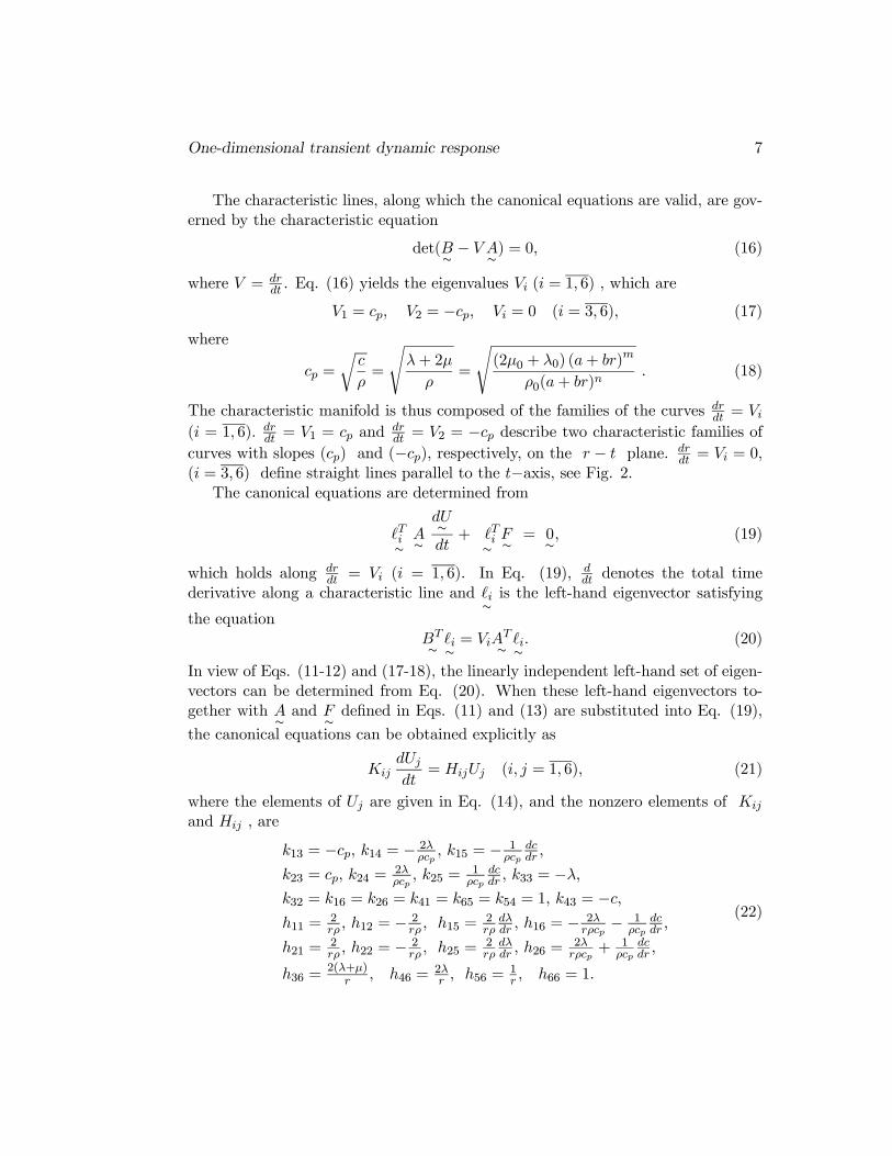
The characteristic lines, along which the canonical equations are valid, are gov-erned by the characteristic equation

det(B∼− V A

∼) = 0, (16)

where V = drdt . Eq. (16) yields the eigenvalues Vi (i = 1, 6) , which are

V1 = cp, V2 = −cp, Vi = 0 (i = 3, 6), (17)

where

cp =

rc

ρ=

sλ+ 2µ

ρ=

s(2µ0 + λ0) (a+ br)m

ρ0(a+ br)n. (18)

The characteristic manifold is thus composed of the families of the curves drdt = Vi

(i = 1, 6). drdt = V1 = cp and dr

dt = V2 = −cp describe two characteristic families ofcurves with slopes (cp) and (−cp), respectively, on the r − t plane. dr

dt = Vi = 0,(i = 3, 6) define straight lines parallel to the t−axis, see Fig. 2.

The canonical equations are determined from

Ti∼

A∼

dU∼dt+ T

i∼

F∼= 0

∼, (19)

which holds along drdt = Vi (i = 1, 6). In Eq. (19), d

dt denotes the total timederivative along a characteristic line and i

∼is the left-hand eigenvector satisfying

the equationBT

∼ i∼= ViA

T

∼ i∼. (20)

In view of Eqs. (11-12) and (17-18), the linearly independent left-hand set of eigen-vectors can be determined from Eq. (20). When these left-hand eigenvectors to-gether with A

∼and F

∼defined in Eqs. (11) and (13) are substituted into Eq. (19),

the canonical equations can be obtained explicitly as

KijdUj

dt= HijUj (i, j = 1, 6), (21)

where the elements of Uj are given in Eq. (14), and the nonzero elements of Kij

and Hij , are

k13 = −cp, k14 = − 2λρcp

, k15 = − 1ρcp

dcdr ,

k23 = cp, k24 =2λρcp

, k25 =1ρcp

dcdr , k33 = −λ,

k32 = k16 = k26 = k41 = k65 = k54 = 1, k43 = −c,h11 =

2rρ , h12 = − 2

rρ , h15 =2rρ

dλdr , h16 = − 2λ

rρcp− 1

ρcpdcdr ,

h21 =2rρ , h22 = − 2

rρ , h25 =2rρ

dλdr , h26 =

2λrρcp

+ 1ρcp

dcdr ,

h36 =2(λ+µ)

r , h46 =2λr , h56 =

1r , h66 = 1.

(22)


Outer boundary )( oRr =

pcdtdr

−=

Typical integration elementt Inner boundary )( Rr =

0=dtdr

pcdtdr

=

r t∆

r∆

1A )63( −=iAi 2A

A

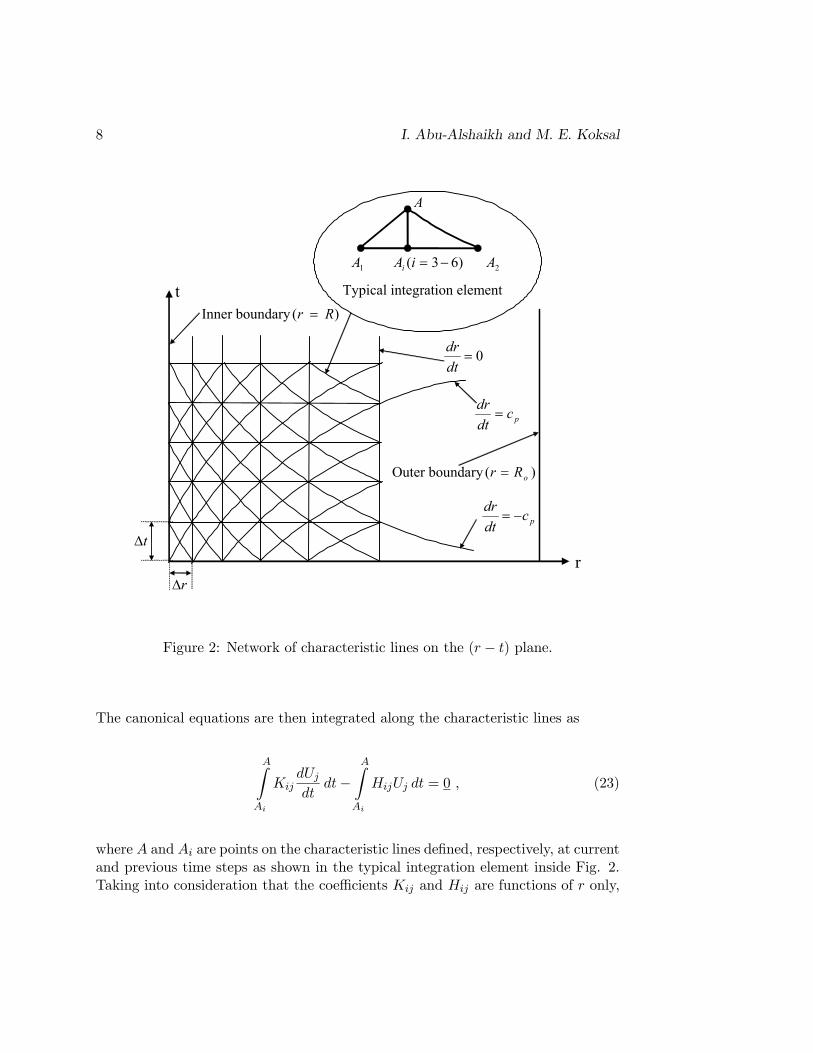
Figure 2: Network of characteristic lines on the (r − t) plane.

The canonical equations are then integrated along the characteristic lines as

AZAi

KijdUj

dtdt−

AZAi

HijUj dt = 0 , (23)

where A and Ai are points on the characteristic lines defined, respectively, at currentand previous time steps as shown in the typical integration element inside Fig. 2.Taking into consideration that the coefficients Kij and Hij are functions of r only,


the above integration can be performed easily by using the trapezoidal rule as [20]

KijUj(A)−KijUj(Ai)−µ∆t

2

¶{Hij(A)Uj(A) +Hij(Ai)UJ(Ai)} = 0 . (24)

Alternately, this equation can be rewritten as

WijUj(A) =MijUj(Ai) (i, j = 1, 6), (25)

where

Wij = Kij −µ∆t

2

¶Hij(A), Mij = Kij +

µ∆t

2

¶Hij(Ai). (26)

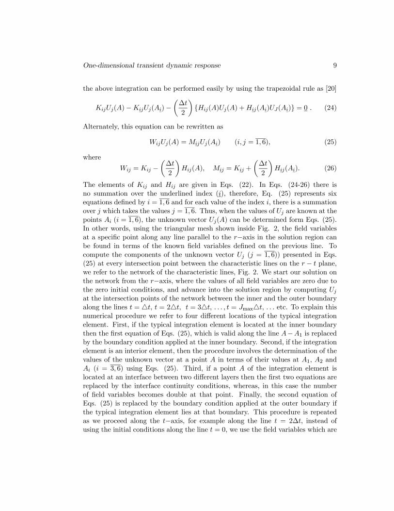
The elements of Kij and Hij are given in Eqs. (22). In Eqs. (24-26) there isno summation over the underlined index (i), therefore, Eq. (25) represents sixequations defined by i = 1, 6 and for each value of the index i, there is a summationover j which takes the values j = 1, 6. Thus, when the values of Uj are known at thepoints Ai (i = 1, 6), the unknown vector Uj(A) can be determined form Eqs. (25).In other words, using the triangular mesh shown inside Fig. 2, the field variablesat a specific point along any line parallel to the r−axis in the solution region canbe found in terms of the known field variables defined on the previous line. Tocompute the components of the unknown vector Uj (j = 1, 6)) presented in Eqs.(25) at every intersection point between the characteristic lines on the r − t plane,we refer to the network of the characteristic lines, Fig. 2. We start our solution onthe network from the r−axis, where the values of all field variables are zero due tothe zero initial conditions, and advance into the solution region by computing Uj

at the intersection points of the network between the inner and the outer boundaryalong the lines t = 4t, t = 24t, t = 34t, . . . , t = Jmax4t, . . . etc. To explain thisnumerical procedure we refer to four different locations of the typical integrationelement. First, if the typical integration element is located at the inner boundarythen the first equation of Eqs. (25), which is valid along the line A−A1 is replacedby the boundary condition applied at the inner boundary. Second, if the integrationelement is an interior element, then the procedure involves the determination of thevalues of the unknown vector at a point A in terms of their values at A1, A2 andAi (i = 3, 6) using Eqs. (25). Third, if a point A of the integration element islocated at an interface between two different layers then the first two equations arereplaced by the interface continuity conditions, whereas, in this case the numberof field variables becomes double at that point. Finally, the second equation ofEqs. (25) is replaced by the boundary condition applied at the outer boundary ifthe typical integration element lies at that boundary. This procedure is repeatedas we proceed along the t−axis, for example along the line t = 2∆t, instead ofusing the initial conditions along the line t = 0, we use the field variables which are


computed in the previous step along the line t = ∆t . This process is repeated untilgetting results for a sufficient value of t, for example t = Jmax4t, where Jmax is themaximum number of intervals considered in the t−direction.

4 Numerical results and discussion

The first example will be given to verify the validity of the numerical techniqueemployed in this study. The numerical results are obtained for a composite bodyconsisting of three pairs of alternating layers, i.e., N = 6. The innermost layer istaken as layer 1, whereas the outermost layer is taken as layer 2, with the layersequence starting from the innermost layer, as 1/2/1/2/1/2, i.e., the third and fifthlayers have the same geometric and material properties as layer 1 and the fourthand sixth layers have the same geometric and material properties as layer 2. Thenon-dimensional material properties for layer 1 and layer 2 are taken as [13]

ρ(1) = 1, µ(1) = 0.254, λ(1) = 0.493,

ρ(2) = 2.9, µ(2) = 0.964, λ(2) = 0.972,(27)

In these non-dimensional quantities, the characteristic length, mass and time aretaken as: the inner radius of the first layer R, the mass density of the first layerρ(1) and R/c

(1)p , where c

(1)p is the dilatational wave velocity in layer 1. In Eq. (27)

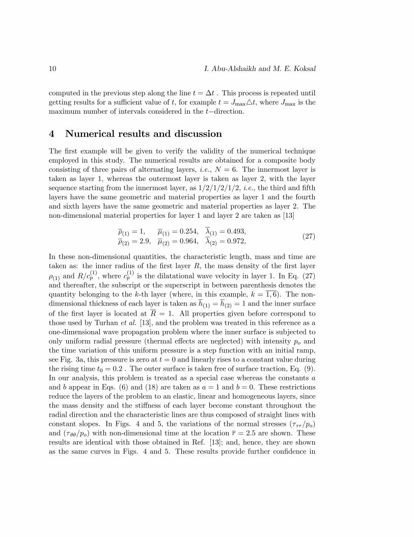
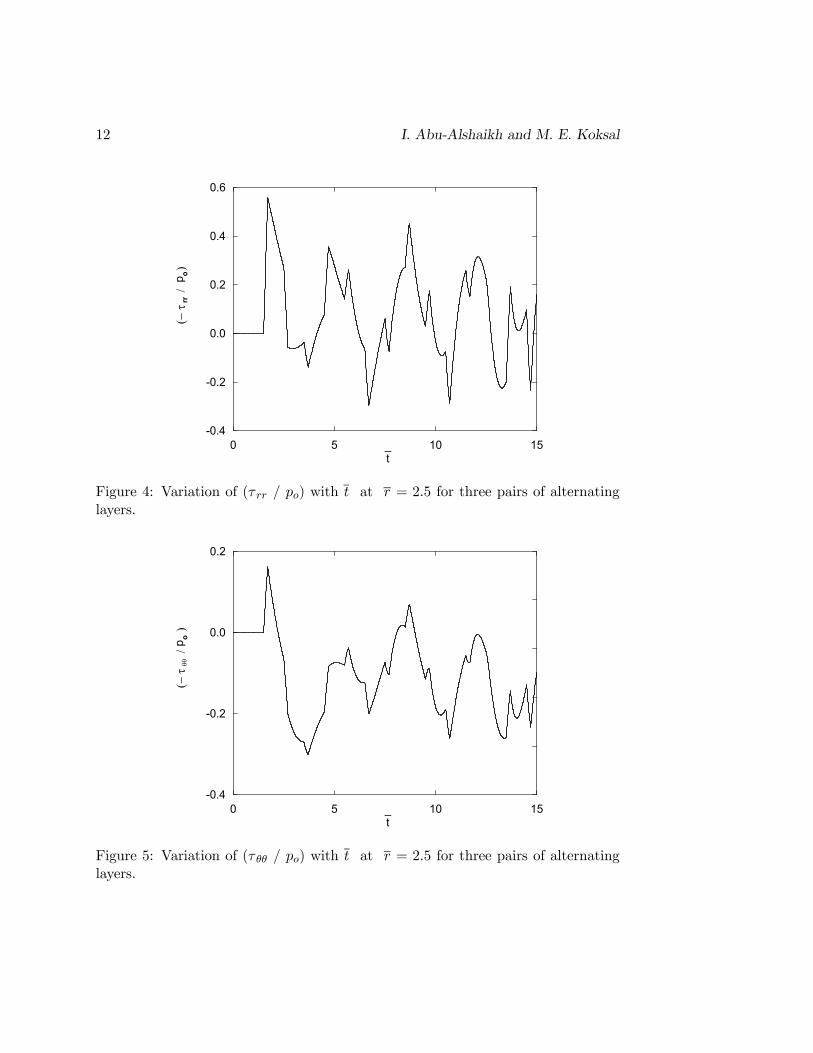
and thereafter, the subscript or the superscript in between parenthesis denotes thequantity belonging to the k-th layer (where, in this example, k = 1, 6). The non-dimensional thickness of each layer is taken as h(1) = h(2) = 1 and the inner surfaceof the first layer is located at R = 1. All properties given before correspond tothose used by Turhan et al. [13], and the problem was treated in this reference as aone-dimensional wave propagation problem where the inner surface is subjected toonly uniform radial pressure (thermal effects are neglected) with intensity po andthe time variation of this uniform pressure is a step function with an initial ramp,see Fig. 3a, this pressure is zero at t = 0 and linearly rises to a constant value duringthe rising time t0 = 0.2 . The outer surface is taken free of surface traction, Eq. (9).In our analysis, this problem is treated as a special case whereas the constants aand b appear in Eqs. (6) and (18) are taken as a = 1 and b = 0. These restrictionsreduce the layers of the problem to an elastic, linear and homogeneous layers, sincethe mass density and the stiffness of each layer become constant throughout theradial direction and the characteristic lines are thus composed of straight lines withconstant slopes. In Figs. 4 and 5, the variations of the normal stresses (τ rr/po)and (τ θθ/po) with non-dimensional time at the location r = 2.5 are shown. Theseresults are identical with those obtained in Ref. [13]; and, hence, they are shownas the same curves in Figs. 4 and 5. These results provide further confidence in


the numerical technique employed in this study to treat transient wave propagationin a spherical FGM layered media. However, we have not found a suitable one-dimensional solutions in a spherical FGM composite for comparison. The curves ofFigs. 4, 5 clearly display the effects of reflections and refractions from the inner andouter boundaries through the large sudden changes in the stress levels, the effectsof reflections and refractions from the interfaces through the small sudden changesin the stress levels. The curves further show the effects of geometric dispersionand show that the numerical technique applied is capable of predicting the sharpvariations in the neighborhood of the wave fronts without showing any sign ofinstability or noise.

0tt

op

)(tf

)(tf

(a)

(b)

0t t∆t∆

opt

Figure 3: Time variations of the loads applied on the inner surface (r = R).

Now, we present some results for one-dimensional wave propagation in an FGMlayer consists of nickel (Ni) and silicon (SiC). On one surface of the layer is purenickel and on the other surface pure silicon, and the material properties in-betweenthese two surfaces vary smoothly in the radial direction. The material propertiesof the constituent materials are given in Table 1. The numerical computationshave been carried out and the results are displayed in terms of non-dimensionalquantities. These dimensionless quantities are taken in terms of the inner radiusR, the density and stiffness at the inner surface, i.e., the following non-dimensionalquantities will be always true on the surface of the inner boundary: R = (2µ+λ) =ρ = 1. Note here that, the non-dimensional quantities are designated by bars. The


0 5 10 15-0.4

-0.2

0.0

0.2

0.4

0.6

t_

(− τ

/

)p

rr

o

Figure 4: Variation of (τ rr / po) with t at r = 2.5 for three pairs of alternatinglayers.

0 5 10 15-0.4

-0.2

0.0

0.2

t_

(− τ

/

)p

oθθ

Figure 5: Variation of (τ θθ / po) with t at r = 2.5 for three pairs of alternatinglayers.


inner surface (r = R = 1) is subjected to a uniform normal stress defined by

τ rr(1, t) = −po (H(t)−H(t− to)) , (28)

where po is the intensity of load and H(t) represents a unit step function with aninitial ramp. Namely, the incident pressure wave applied on the inner surface isequivalent to the trapezoidal distribution shown in Fig. 3b, where t0 and 4t aretaken as 0.25 and 0.001, respectively.

Table 1. Properties of materials used in examples.µ(GPa) λ(GPa) ρ(Kg/m3)

Ni (Nickel) 79 129 8900SiC (Silicon) 90 46 3100

Here, we consider four different problems, all are subject to the trapezoidalpulse given by Eq. (28) and shown in Fig. 3b. These problems are: nickel-silicon(Ni/SiC) or silicon-nickel (SiC/Ni) FGM layer with free or fixed outer boundaryconditions. The FGM spherical layer is assumed to be consisting of four similarlayers with h(k) = 0.25 (k = 1, 4), where h(k) is the non-dimensional thickness ofthe k-th layer, see Fig. 6. The thicknesses and the material properties of all thefour layers are assumed to be the same. Thus, using the non-dimensionalization,the material properties defined by Eq. (6) for the four layers can be computed fromTable 1 as:

for the Ni/SiC FGM layer with m = n+ 2, see Fig. 6a,

m = −0.58585, n = −2.58585, a = 0.4964, b = 0.5036,

ρ0 = 1, µ0 = 0.27526, λ0 = 0.44948, c0 = 1,(29)

and for the SiC/Ni FGM layer with m = n+ 2, see Fig. 6b,

m = −0.58588, n = −2.58588, a = 1.33492, b = −0.33492,ρ0 = 1, µ0 = 0.39823, λ0 = 0.20354, c0 = 1.

(30)

For various combinations of boundary conditions and material compositionsshown in Fig. 6, the variation of normalized normal stresses τ rr/po and τ θθ/powith the non-dimensional time t at r = 1.25 is given in Figs. 7—12. The curves inFigs. 7—10, correspond to free outer boundary conditions, while the curves of Figs.11, 12 correspond to fixed outer boundary conditions. The dashed curves in thesefigures, Figs. 7—12, correspond to FGM layers with material properties given inEq. (29) or (30), whereas the solid curves correspond to linear, homogeneous and


1.00 1.25 1.50 1.75 2.000.5

1.0

1.5

2.0

2.5

3.0

1 2 3 4

c

_

SiC Ni r

(b)

_

-

1.00 1.25 1.50 1.75 2.00

0.4

0.8

1.2

1.6

1 2 3 4

(a)

Ni SiC

ρ-

c-

ρ

r-

c p-

c p-

Figure 6: Variation of non-dimensional density (ρ = ρρ0), stiffness (c = 2µ+λ

2µ0+λ0) and

wave velocity (cp) with r in (a) Ni/SiC FGM composite and (b) SiC/Ni FGMcomposite.

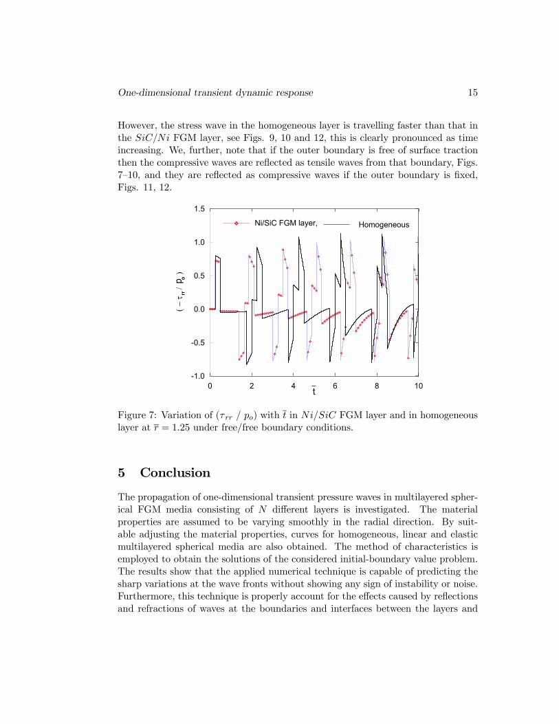
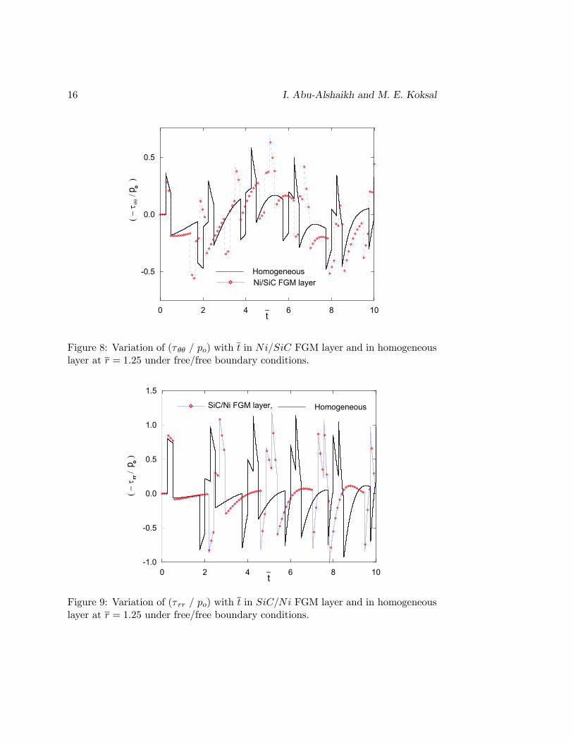
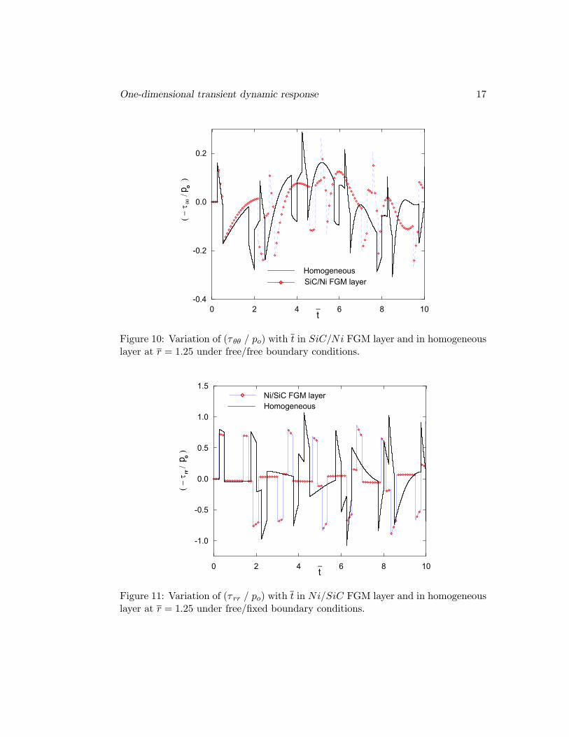
isotropic material. Since the properties of all the four layers are taken equal, thedashed curves in Figs. 7—12 represent solutions for a single FGM spherical layerwith dimensionless outer boundary Ro = 2 and with material properties given inEq. (29) or Eq. (30). The curves corresponding to the homogeneous layer areobtained as a special case by assigning a = 1 and b = 0 in Eqs. (29—30); whereas,the propagation time of the dilatational wave (cp) through the non-dimensionalthickness (Ro − R = 1) of the homogeneous layer is taken as t = 1. The curvesof Figs. 7—12 clearly show the effects of reflections at the inner and outer surfacesthrough the sudden changes in the stress levels. We note further that reflectionsand refractions from the interfaces have disappeared, this is due to the fact that thematerial properties vary smoothly in the radial direction. Moreover, we note thatthe stress levels in the homogeneous layer are higher than those correspond to theNi/SiC FGM layer, Figs. 7, 8 and 11, and they are less than those correspond tothe SiC/Ni FGM layer, Figs. 9, 10 and 12. These deviations from the homogeneousmaterial are due to the fact that the inner boundary r = 1 is the stiffer side in theNi/SiC FGM layer, Fig. 6a, and if r = 1 is the less stiff side, then the stress levelswill be higher than the corresponding homogeneous layer. Because the wave velocityof the homogeneous layer (cp = 1) is less than that of the Ni/SiC FGM layer, Fig.6a, the stress wave propagates faster in the Ni/SiC FGM layer, Figs. 7, 8 and 11.


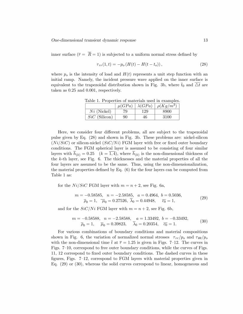
However, the stress wave in the homogeneous layer is travelling faster than that inthe SiC/Ni FGM layer, see Figs. 9, 10 and 12, this is clearly pronounced as timeincreasing. We, further, note that if the outer boundary is free of surface tractionthen the compressive waves are reflected as tensile waves from that boundary, Figs.7—10, and they are reflected as compressive waves if the outer boundary is fixed,Figs. 11, 12.

0 2 4 6 8 10-1.0

-0.5

0.0

0.5

1.0

1.5

t_

( − τ

/

)

prr

o

Ni/SiC FGM layer, Homogeneous

Figure 7: Variation of (τ rr / po) with t in Ni/SiC FGM layer and in homogeneouslayer at r = 1.25 under free/free boundary conditions.

5 Conclusion

The propagation of one-dimensional transient pressure waves in multilayered spher-ical FGM media consisting of N different layers is investigated. The materialproperties are assumed to be varying smoothly in the radial direction. By suit-able adjusting the material properties, curves for homogeneous, linear and elasticmultilayered spherical media are also obtained. The method of characteristics isemployed to obtain the solutions of the considered initial-boundary value problem.The results show that the applied numerical technique is capable of predicting thesharp variations at the wave fronts without showing any sign of instability or noise.Furthermore, this technique is properly account for the effects caused by reflectionsand refractions of waves at the boundaries and interfaces between the layers and


0 2 4 6 8 10

-0.5

0.0

0.5

t_

( − τ

/

)

p

o

Ni/SiC FGM layerHomogeneous

θθ

Figure 8: Variation of (τ θθ / po) with t in Ni/SiC FGM layer and in homogeneouslayer at r = 1.25 under free/free boundary conditions.

0 2 4 6 8 10-1.0

-0.5

0.0

0.5

1.0

1.5

t_

( − τ

/

)

prr

o

SiC/Ni FGM layer, Homogeneous

Figure 9: Variation of (τ rr / po) with t in SiC/Ni FGM layer and in homogeneouslayer at r = 1.25 under free/free boundary conditions.


0 2 4 6 8 10-0.4

-0.2

0.0

0.2

t_

( − τ

/

)

p

o

SiC/Ni FGM layerHomogeneous

θθ

Figure 10: Variation of (τ θθ / po) with t in SiC/Ni FGM layer and in homogeneouslayer at r = 1.25 under free/free boundary conditions.

0 2 4 6 8 10

-1.0

-0.5

0.0

0.5

1.0

1.5

t_

( − τ

/

)

prr

o

Ni/SiC FGM layerHomogeneous

Figure 11: Variation of (τ rr / po) with t in Ni/SiC FGM layer and in homogeneouslayer at r = 1.25 under free/fixed boundary conditions.


0 2 4 6 8 10

-1.0

-0.5

0.0

0.5

1.0

1.5

t_

( − τ

/

)

prr

oSiC/Ni FGM layerHomogeneous

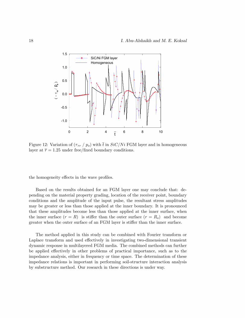
Figure 12: Variation of (τ rr / po) with t in SiC/Ni FGM layer and in homogeneouslayer at r = 1.25 under free/fixed boundary conditions.

the homogeneity effects in the wave profiles.

Based on the results obtained for an FGM layer one may conclude that: de-pending on the material property grading, location of the receiver point, boundaryconditions and the amplitude of the input pulse, the resultant stress amplitudesmay be greater or less than those applied at the inner boundary. It is pronouncedthat these amplitudes become less than those applied at the inner surface, whenthe inner surface (r = R) is stiffer than the outer surface (r = Ro) and becomegreater when the outer surface of an FGM layer is stiffer than the inner surface.

The method applied in this study can be combined with Fourier transform orLaplace transform and used effectively in investigating two-dimensional transientdynamic response in multilayered FGM media. The combined methods can furtherbe applied effectively in other problems of practical importance, such as to theimpedance analysis, either in frequency or time space. The determination of theseimpedance relations is important in performing soil-structure interaction analysisby substructure method. Our research in these directions is under way.


Acknowledgement

The authors would like to thank Dr. Ali Sahin, for his valuable suggestions and Mr.Ibrahim Karatay who assisted in preparing the manuscript.

References

[1] Yamanouchi M., Koizumi M., Hirai T. and Shiota I., Proceedings of the FirstInternational Symposium on Functionally Graded Materials, 1990.

[2] Koizumu M. The concept of FGM, Ceram. Trans. Funct. Grad. Mater., 34 (1993),3—10.

[3] Banks-Sills L., Eliasi R. and Berlin Y., Modeling of functionally graded mate-rials in dynamic analyses, Composites Part B: Engineering, 33 (2002), 7—15, 2002.

[4] Liu G. R. and Tani J., Surface waves in funtionally gradient piezoelectric plates,Journal of Vibration and Acoustics, 116 (1994), 440—448.

[5] Ohyoshi T., Linearly inhomogeneous layer elements for reflectance evaluation of in-homogeneous layers, Dynamic Response and Behavior of Composites, 46 (1995), 121—126.

[6] Ohyoshi T., New stacking layer elements for analyses of reflection and transmissionof elastic waves to inhomogeneous layers, Mechanics Research Communication, 20(1993), 353—359.

[7] Han X. and Liu G. R., Effects of waves in functionally graded plate, MechanicsResearch Communication, 29 (2002), 327—338.

[8] Liu G. R., Han X. and Lam K. Y., Stress Waves in functionally gradient materialsand its use for material characterization, Composites Part B: Engineering, 30 (1999),383—394.

[9] Han X., Liu G. R. and Lam K. Y., A quadratic layer element for analyzing stresswaves in functionally gradient materials and its application in material characteriza-tion, Journal of Sound and Vibration, 236 (2000), 307—321.

[10] Chiu T. C. and Erdogan F., One-dimensional wave propagation in a functionallygraded elastic medium, Journal of Sound and Vibration, 222 (1999), 453—487.

[11] Berezovski A., Engelbrecht J. and Maugin G. A., Numerical simulation oftwo dimensional wave propagation in functionally graded materials, European Journalof Mechanics, 22 (2003), 257—265.

[12] Santare M. H., Thamburaj P. and Gazoans G. A., The use of graded finiteelements in the study of elastic wave propagation in continuously non-homogeneousmaterials, International Journal of Solids and Structures, 40 (2003), 5621—5634.


[13] Turhan D., Celep Z. and Zain-eddin I. K., Transient wave propagation in layeredmedia Journal of Sound and Vibration, 144 (1991), 247—261.

[14] Mengi Y. and Tanr¬kulu A. K., A numerical technique for two-dimensional tran-sient wave propagation analyses, Communication of Applied Numerical Methods, 6(1990), 623—632.

[15] Wegner J. L., Propagation of waves from a spherical cavity in an unbounded linearviscoelastic solid, International Journal of Engineering Sciences, 31 (1993), 493—508.

[16] Abu-Alshaikh I., Turhan D. and Mengi Y., Two-dimensional transient wavepropagation in viscoelastic layered media, Journal of Sound and Vibration, 244 (2001),837—858.

[17] Abu-Alshaikh I., Turhan D. and Mengi Y., Transient waves in viscoelastic cylin-drical layered media, European Journal Mechanics A/Solids 21 (2002), 811—830.

[18] Courant R. and Hilbert D.,Methods of Mathematical Physics Vol. II., IntersciencePublishers, New York, 1966.

[19] Whitham G. B., Linear and Nonlinear Waves, Wiley, New York, 1974.

[20] Gerald C. F. and Wheately P. O., Applied Numerical Analysis, USA, 1984.

one-dimensional transient dynamic response of functionally

Documents