one and two dimensional fourier analysis

One and Two Dimensional Fourier Analysis

Tolga Tasdizen ECE

University of Utah

1

2

Fourier Series

•  J. B. Joseph Fourier, 1807 – Any periodic function

can be expressed as a weighted sum of sines and/or cosines of different frequencies.

© 1992–2008 R. C. Gonzalez & R. E. Woods

What is the period of this function?

3

Fourier Series •  f(t) periodic

signal with period T

•  Frequency of sines and cosines

3

The complex exponentials form an orthogonal basis for the range [-T/2,T/2] or any other interval with length T such as [0,T]

4

Types of functions Continuous f(t)

Discrete f(n)

Periodic Fourier series Discrete Fourier series

Non-periodic Fourier transform

Discrete Fourier transform

5

Fourier Transform Pair

•  The domain of the Fourier transform is the frequency domain. –  If t is in seconds, mu is in Hertz (1/seconds)

•  The function f(t) can be recovered from its Fourier transform.

6

Fourier Transform example

•  Fourier transform of the box function is the sinc function.

•  In general, the Fourier transform is a complex quantity. In this case it is real.

•  The magnitude of the Fourier transform is a real quantity, called the Fourier spectrum (or frequency spectrum).


7

Convolution and Fourier Trans.

Can see this by change of variables t’ = t - Τ

8

•  Convolution in time domain is multiplication in frequency domain

•  Multiplication in time domain is convolution in frequency domain

9

Unit impulse function

•  Properties – Unit area

– Sifting

9

10

Unit discrete impulse

•  x: Discrete variable

•  Properties

10

11

Fourier Transform of Impulses

12

Impulse train

•  Periodic function (period = ΔT) so can be represented as a Fourier sum

12 © 1992–2008 R. C. Gonzalez & R. E. Woods

13

Fourier Trans. of Impulse Train Substitute for cn

Linearity of Fourier transform Duality FT of an impulse train is an impuse train!

13

14

Proof of duality for impulses From before Take Fourier Trans. of both sides

Discrete Sampling and Aliasing

•  Digital signals and images are discrete representations of the real world – Which is continuous

•  What happens to signals/images when we sample them? – Can we quantify the effects? – Can we understand the artifacts and can we limit

them? – Can we reconstruct the original image from the

discrete data? 15

16

Sampling

•  We can sample continuous function f(t) by multiplication with an impulse train


17

Fourier trans. of sampled func.

•  What does this mean? 17

Fourier Transform of A Discrete Sampling

18

u

Fourier Transform of A Discrete Sampling

u

Energy from higher freqs gets folded back down into lower freqs – Aliasing

Frequencies get mixed. The original signal is not recoverable.

What if F(u) is Narrower in the Fourier Domain? •  No aliasing! •  How could we recover the original signal?

20

u

21

•  Fourier transform of band-limited signal

•  Over-sampling

•  Critically-sampling

•  Under-sampling


What Comes Out of This Model

•  Sampling criterion for complete recovery •  An understanding of the effects of sampling

– Aliasing and how to avoid it •  Reconstruction of signals from discrete samples

22

23

Sampling theorem

•  When can we recover f(t) from its sampled version? –  f(t) has to be band-

limited –  If we can isolate a

single copy of F(µ) from the Fourier transform of the sampled signal. Nyquist rate


Sampling Theorem

•  Quantifies the amount of information in a signal – Discrete signal contains limited frequencies – Band-limited signals contain no more information then

their discrete equivalents •  Reconstruction by cutting away the repeated

signals in the Fourier domain – Convolution with sinc function in space/time

24

25

Function recovery from sample


What is this function in time? It is a sinc function

Reconstruction

•  Convolution with sinc function

26

rect (�Tu)

Note: Sinc function has infinite duration. Why? Ideal reconstruction is not feasible in practice What happens if you truncate the sinc?

27

Aliasing example


Figure: Sampling rate less than Nyquist rate

f (t) = sin(πt)

Period = 2, Frequency = 0.5 Nyquist rate = 2 x 0.5 = 1

Sampling rate must be strictly greater than the Nyquist rate. What happens if we sample this signal at exactly the Nyquist rate?

28

Inevitable aliasing

•  No function of finite duration can be band-limited!!

•  Assume we have a band-limited signal of infinite duration. We limit the duration by multiplication with a box function: – We already know the Fourier transform of

the box function is a sinc function in frequency domain which extends to infinity.

– Multiplication in time domain is convolution in frequency domain. Therefore, we destroyed the band-limited property of the original signal

29

Two-dimensional Fourier Transform Pair

Properties from 1D carry over to 2D: Shifting in space <-> Multiplication with a complex exponential Duality of multiplication and convolution Etc..

30

2D impulse function

30 6

31

2D sampling

•  2D impulse train as sampling function

•  Sampling theorem – Band-limited

– Sampling rate limits

31

32

Aliasing in images

Over-sampled Under-sampled Aliasing


33

Aliasing example

•  Digitizing a checkerboard pattern with 96 x 96 sample array. –  We can resolve squares that have physical sides one

pixel long or longer


16 pixels 8 pixels

0.9174 pixels

0.4798 pixels

34

Aliasing in images

•  No time or space limited signal can be band limited

•  Images always have finite extent (duration) so aliasing is always present

•  Effects of aliasing can be reduced by slightly defocusing the scene to be digitized (blurring continuous signal)

•  Resampling a digital image can also cause aliasing. – Blurring (averaging) helps reduce these

effects

Overcoming Aliasing

•  Filter data prior to sampling –  Ideally - band limit the data (conv with sinc function) –  In practice - limit effects with fuzzy/soft low pass

35

36

Overcoming alising due to image resampling


37

Discrete Fourier Transform

•  Fourier transform of sampled data was derived in terms of the transform of the original function:

•  We want an expression in terms of the sampled function itself. From the definition of the Fourier Transform:

37

39

Discrete Fourier Trans. (DFT)

•  Notice that the Fourier transform of the discrete signal fn is continuous and periodic! What is the period?

•  We only need to sample one period of the Fourier transform. This is the DFT:

– Samples taken at

– m=0,1,...,M-1 39

40

Discrete Fourier Transform Pair

m=0,1,...,M-1 n=0,1,...,M-1

40

Discrete signal f0, …, fM-1

41

2D Discrete Fourier Transform

• Notation: From now on we will use x,y and u,v to denote discrete variables.

• f(x,y) is a M x N digital image • F(u,v) is also a 2D matrix of size M x N. Its elements are complex quantities.

42

Spatial and frequency intervals

•  The entire range of frequencies spanned by the DFT is

•  The relationship between the spatial and frequency intervals is

42

43

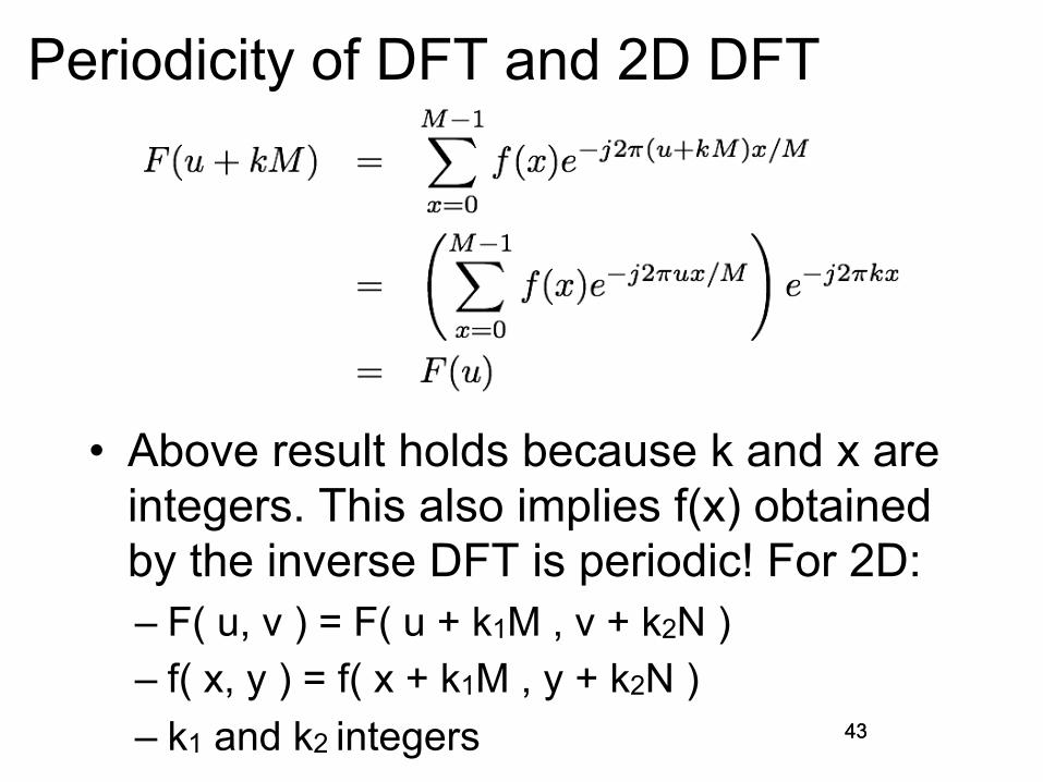
Periodicity of DFT and 2D DFT

•  Above result holds because k and x are integers. This also implies f(x) obtained by the inverse DFT is periodic! For 2D: – F( u, v ) = F( u + k1M , v + k2N ) –  f( x, y ) = f( x + k1M , y + k2N ) – k1 and k2 integers 43

44

Fourier spectrum and phase

•  Since the DFT is a complex quantity it can also be expressed in polar coordinates:

44 4-quadrant arctangent, atan2 command in MATLAB

Fourier Spectrum

45

Fourier spectrum Origin in corners

Retiled with origin In center

Log of spectrum

Image

46

Translation properties

•  Translation in space

•  Translation in frequency

46

Note: Centering the Fourier transform is a shift in frequency with u0 = M/2 and v0 = N/2 which is a multiplication by (-1)x+y in space

47

Centering the DFT

We want half period (M/2) shift in the frequency domain:

48

In 2D...

49

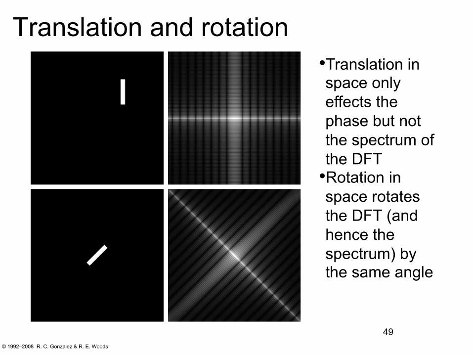
Translation and rotation


• Translation in space only effects the phase but not the spectrum of the DFT

• Rotation in space rotates the DFT (and hence the spectrum) by the same angle

50

Phase information

•  Phase angle is not intuitive, but it is critical. It determines how the various frequency sinusoids add up. This gives result to shape! 50


51

Importance of phase angle


one and two dimensional fourier analysis

Documents