Naval Research LaboratoryWashington, DC 20375-5320

NRL/MR/6410--09-9188

Onboard Stability Control System for a Flapping Wing Nano Air VehicleJason Geder

Center for Reactive Flow and Dynamical Systems Laboratory for Computational Physics and Fluid Dynamics

April 24, 2009

Approved for public release; distribution is unlimited.

i

REPORT DOCUMENTATION PAGE Form ApprovedOMB No. 0704-0188

3. DATES COVERED (From - To)

Standard Form 298 (Rev. 8-98)Prescribed by ANSI Std. Z39.18

Public reporting burden for this collection of information is estimated to average 1 hour per response, including the time for reviewing instructions, searching existing data sources, gathering and maintaining the data needed, and completing and reviewing this collection of information. Send comments regarding this burden estimate or any other aspect of this collection of information, including suggestions for reducing this burden to Department of Defense, Washington Headquarters Services, Directorate for Information Operations and Reports (0704-0188), 1215 Jefferson Davis Highway, Suite 1204, Arlington, VA 22202-4302. Respondents should be aware that notwithstanding any other provision of law, no person shall be subject to any penalty for failing to comply with a collection of information if it does not display a currently valid OMB control number. PLEASE DO NOT RETURN YOUR FORM TO THE ABOVE ADDRESS.

5a. CONTRACT NUMBER

5b. GRANT NUMBER

5c. PROGRAM ELEMENT NUMBER

5d. PROJECT NUMBER

5e. TASK NUMBER

5f. WORK UNIT NUMBER

2. REPORT TYPE1. REPORT DATE (DD-MM-YYYY)

4. TITLE AND SUBTITLE

6. AUTHOR(S)

8. PERFORMING ORGANIZATION REPORT NUMBER

7. PERFORMING ORGANIZATION NAME(S) AND ADDRESS(ES)

10. SPONSOR / MONITOR’S ACRONYM(S)9. SPONSORING / MONITORING AGENCY NAME(S) AND ADDRESS(ES)

11. SPONSOR / MONITOR’S REPORT NUMBER(S)

12. DISTRIBUTION / AVAILABILITY STATEMENT

13. SUPPLEMENTARY NOTES

14. ABSTRACT

15. SUBJECT TERMS

16. SECURITY CLASSIFICATION OF:

a. REPORT

19a. NAME OF RESPONSIBLE PERSON

19b. TELEPHONE NUMBER (include areacode)

b. ABSTRACT c. THIS PAGE

18. NUMBEROF PAGES

17. LIMITATIONOF ABSTRACT

Onboard Stability Control System for a Flapping Wing Nano Air Vehicle

Jason Geder

Naval Research Laboratory4555 Overlook Avenue, SWWashington, DC 20375-5320

NRL/MR/6410--09-9188

DARPA

Approved for public release; distribution is unlimited.

Unclassified Unclassified UnclassifiedUL 21

Jason Geder

(202) 767-1975

Nano air vehicleFeedback control

This paper describes the design and development of a feedback system for controlling the dynamics of a flapping wing nano air vehicle (NAV). A model of the vehicle dynamics and models of sensors and unique actuator mechanisms are built. An extended Kalman filter is designed to eliminate the effects of sensor bias on state estimation. Results of this study demonstrate stability and yield vehicle responses that are approaching desired performance capabilities.

24-04-2009 Memorandum Report

Kalman filterFlapping flight

64-9173-0-7

Bio-inspired flight

iii

Table of Contents

INTRODUCTION......................................................................................................................... 1

THE CASE FOR FLAPPING FLIGHT..................................................................................... 1

SYSTEM ARCHITECTURE AND COORDINATE FRAMES .............................................. 2

ONBOARD STABILITY CONTROL SUBCOMPONENTS................................................... 3

Onboard Stability Sensors .......................................................................................................... 3

Stability Control Algorithms ....................................................................................................... 4

Wing Control Actuators .............................................................................................................. 5

NAV MODEL................................................................................................................................ 8

RESULTS .................................................................................................................................... 11

DISCUSSION .............................................................................................................................. 18

ACKNOWLEDGMENTS .......................................................................................................... 18

REFERENCES............................................................................................................................ 18

List of Figures

Figure 1. Onboard stability control system block diagram............................................................ 2 Figure 2. Earth-fixed and body-fixed coordinate frames............................................................... 3 Figure 3. Positive rotations of the bug’s pitch (θ), functional roll (ψ ) and functional yaw (ϕ) ... 3 Figure 4. The stroke mean position is used to control the bug’s forward speed. The stroke

amplitude is used to control the bug’s lateral speeds. The stroke plane angle is used to control NAV turning rates. ..................................................................................................... 5

Figure 5. Wing wedges for controlling the stroke amplitude and mean position .......................... 6 Figure 6. Mechanisms for controlling pitch, functional roll, and functional yaw ......................... 7 Figure 7. Aerodynamic forces on the wings throughout a stroke .................................................. 8 Figure 8. SimulinkTM block diagram of the feedback control loop ............................................... 9 Figure 9. An illustrative example of vehicle pitch angle estimate from extended Kalman filter 11 Figure 10. Vehicle response to position commands in the x-z plane........................................... 12 Figure 11. Vehicle response to forward speed command of 4.5 m/s........................................... 13 Figure 12. Vehicle in hover: response to functional yaw command of 7.5 degrees with perfect

actuators ................................................................................................................................ 14 Figure 13. Vehicle at 2 m/s forward speed: response to functional yaw command of 7.5 degrees

with perfect actuators ............................................................................................................ 15 Figure 14. Vehicle response to hover command with nitinol actuators and sensors modeled. An

extended Kalman filter has been implemented to estimate the functional roll rate from gyro and accelerometer measurements.......................................................................................... 16

Figure 15. Vehicle response to functional yaw command of 7.5 degrees with nitinol actuators and sensors modeled. An extended Kalman filter has been implemented to estimate the functional roll rate from sensor measurements ..................................................................... 17

___________________ Manuscript approved February 12, 2009.

Onboard Stability Control System for a Flapping Wing Nano Air Vehicle

INTRODUCTION

This paper describes the development of an onboard stability control system for a small flapping-wing nano air vehicle (NAV). It details the creation of control algorithms to be used with the onboard sensors and unique control actuators required for such a flapping-wing vehicle. Simulations to validate this control system based on a wing modulation actuation scheme are discussed.

The onboard stability control system consists of hardware and software components onboard the NAV. Onboard hardware includes onboard stability sensors and wing control actuators. Onboard software includes the stability control algorithms, which are programmed onto a microprocessor chip to compute the necessary actuator commands based on sensor data.

The onboard stability control system provides the means by which the NAV responds to guidance commands to complete various stages of a mission. This system accepts inputs regarding the current flight mode of the vehicle, and utilizes sensory information detailing position, orientation, and motion to determine commands for the control actuation mechanisms. Using an extended Kalman filter, simulation results demonstrate that real data from a one-eighth gram gyroscope and a one-thirtieth gram accelerometer on a flapping aircraft, along with position updates from a ground-based guidance system, could deliver adequate sensory input for controlled precision maneuvers.

The NAV operates in two modes depending on the mission stage: autopilot mode and teleoperator mode. During the autopilot mode of the mission, the operator has no direct control over the vehicle motion. Inputs in autopilot mode are taken from preprogrammed targets, offboard guidance updates, and onboard stability sensors. During the teleoperator stages of the mission, the operator directly controls the maneuvering commands. Inputs in teleoperator mode are taken from operator stick movements and onboard stability sensors. The functioning of the onboard stability control system is transparent to the operator. THE CASE FOR FLAPPING FLIGHT

Flapping-winged vehicles hold the promise of controlling transient dynamics to enable the

ability to conquer gusts. Because these adverse flow regimes come about precisely within the types of missions that are of interest for small hoverers, such as flying through urban canyons, maneuvering indoors in cluttered environments, or perching and landing on windowsills, finding novel solutions to deal with these types of flow is essential.

Insects achieve extremely high turn rates – up to 10π radians per second – solely by modulating their wings, without tail rudder or elevator assistance. Insects can perform highly acrobatic maneuvers because they can independently modulate their left and right wings. With just a few degrees of tilt difference between left and right wingstroke planes, they can maneuver unlike any man-made aircraft. The same controllability that enables such extreme agility also provides the solution to flying through urban canyons. Helicopters do not have this left-right wing articulation which is the key to countering gusts in such environments.

We take the bold approach unlike conventional ornithopters, of stabilizing a flapper without a tail surface in order to reach for the highest levels of agility. While flapping propulsion endows

1

2

small hoverers with remarkable ability as nature has proven, man-made aircraft flapping is the least well understood form of aerial propulsion. Today we have no design tools for flapping aircraft, and unsteady aerodynamics is still a field of many unanswered scientific questions. SYSTEM ARCHITECTURE AND COORDINATE FRAMES

Within each of the stages of the NAV mission, various control maneuvers are needed. These maneuvers include hover,

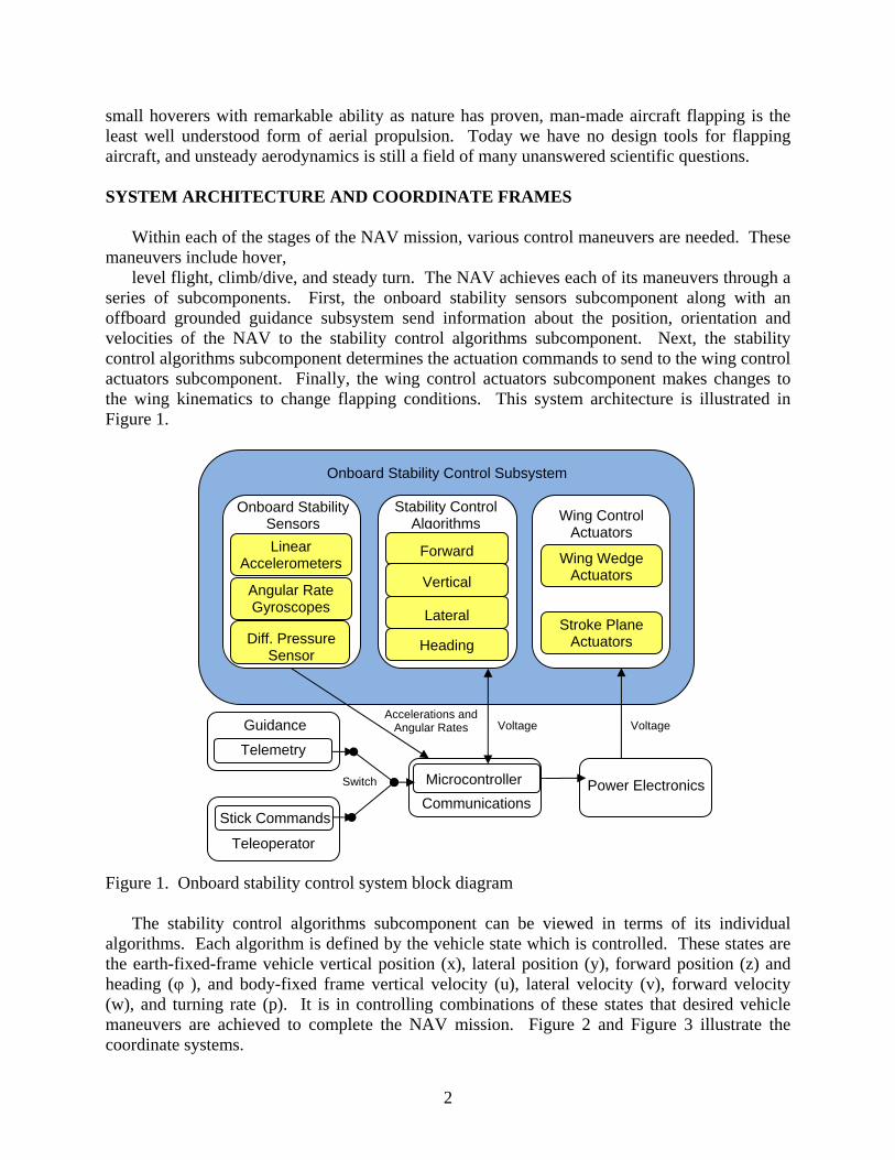
level flight, climb/dive, and steady turn. The NAV achieves each of its maneuvers through a series of subcomponents. First, the onboard stability sensors subcomponent along with an offboard grounded guidance subsystem send information about the position, orientation and velocities of the NAV to the stability control algorithms subcomponent. Next, the stability control algorithms subcomponent determines the actuation commands to send to the wing control actuators subcomponent. Finally, the wing control actuators subcomponent makes changes to the wing kinematics to change flapping conditions. This system architecture is illustrated in Figure 1.

Figure 1. Onboard stability control system block diagram The stability control algorithms subcomponent can be viewed in terms of its individual

algorithms. Each algorithm is defined by the vehicle state which is controlled. These states are the earth-fixed-frame vehicle vertical position (x), lateral position (y), forward position (z) and heading (φ ), and body-fixed frame vertical velocity (u), lateral velocity (v), forward velocity (w), and turning rate (p). It is in controlling combinations of these states that desired vehicle maneuvers are achieved to complete the NAV mission. Figure 2 and Figure 3 illustrate the coordinate systems.

Onboard Stability Control Subsystem

Onboard Stability Sensors

Stability Control Algorithms Wing Control

Actuators Linear

Accelerometers

Angular Rate Gyroscopes

Forward

Vertical

Lateral

Heading

Wing Wedge Actuators

Stroke Plane Actuators

Guidance

Telemetry

Stick Commands

Teleoperator

MicrocontrollerCommunications

Power Electronics Switch

Accelerations and Angular Rates Voltage Voltage

Diff. Pressure Sensor

3

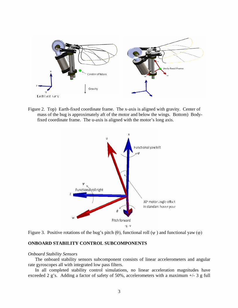
Figure 2. Top) Earth-fixed coordinate frame. The x-axis is aligned with gravity. Center of mass of the bug is approximately aft of the motor and below the wings. Bottom) Body-fixed coordinate frame. The u-axis is aligned with the motor’s long axis.

Figure 3. Positive rotations of the bug’s pitch (θ), functional roll (ψ ) and functional yaw (ϕ) ONBOARD STABILITY CONTROL SUBCOMPONENTS Onboard Stability Sensors

The onboard stability sensors subcomponent consists of linear accelerometers and angular rate gyroscopes all with integrated low pass filters.

In all completed stability control simulations, no linear acceleration magnitudes have exceeded 2 g’s. Adding a factor of safety of 50%, accelerometers with a maximum +/- 3 g full

4

scale range will be sufficient for use on the NAV. The ST Microelectronics LIS302DL 3-axis accelerometer meets this requirement with a +/- 8 g full scale range. This device measures linear accelerations in the x-, y-, and z-axis body frame, and reduces high frequency fluctuations due to noise and oscillation caused by high frequency wing flapping. The 400 Hz data output rate, 200 Hz cutoff frequency, and noise characteristics of the accelerometer have been modeled in the stability control simulation and provide fast enough updates for stable response. Additional filtering may be necessary in the control algorithm subcomponent, as specifics regarding data filtering on the accelerometer have been unavailable. These measured accelerations can be integrated to get vehicle linear velocities.

In all completed stability control simulations, no angular velocity magnitudes have exceeded 250 degrees per second (°/s). Adding a factor of safety of 50%, gyroscopes with a maximum +/- 375 °/s full scale range will be sufficient for use on the NAV. The InvenSense IDG-1004 integrated dual-axis gyroscope meets this requirement with a +/- 1000 °/s full scale range. Two of these devices allow measurement of the roll, pitch, and yaw angular velocities, and reduce high frequency fluctuations due to noise and oscillation caused by high frequency wing flapping. An achievable 400 Hz output data rate, 140 Hz cutoff frequency, and noise characteristics have been modeled in the stability control simulation and provide fast enough updates for stable response. Stability Control Algorithms

The stability control algorithms subcomponent is onboard software which serves as a data interface. It consists of algorithms for various operational modes. Each of these algorithms includes a:

Forward speed or position controller This portion of the algorithm accepts either a forward speed or position command in

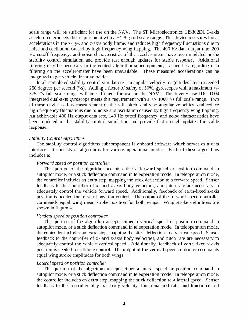
autopilot mode, or a stick deflection command in teleoperation mode. In teleoperation mode, the controller includes an extra step, mapping the stick deflection to a forward speed. Sensor feedback to the controller of x- and z-axis body velocities, and pitch rate are necessary to adequately control the vehicle forward speed. Additionally, feedback of earth-fixed z-axis position is needed for forward position control. The output of the forward speed controller commands equal wing mean stroke position for both wings. Wing stroke definitions are shown in Figure 4.

Vertical speed or position controller This portion of the algorithm accepts either a vertical speed or position command in

autopilot mode, or a stick deflection command in teleoperation mode. In teleoperation mode, the controller includes an extra step, mapping the stick deflection to a vertical speed. Sensor feedback to the controller of x- and z-axis body velocities, and pitch rate are necessary to adequately control the vehicle vertical speed. Additionally, feedback of earth-fixed x-axis position is needed for altitude control. The output of the vertical speed controller commands equal wing stroke amplitudes for both wings.

Lateral speed or position controller This portion of the algorithm accepts either a lateral speed or position command in

autopilot mode, or a stick deflection command in teleoperation mode. In teleoperation mode, the controller includes an extra step, mapping the stick deflection to a lateral speed. Sensor feedback to the controller of y-axis body velocity, functional roll rate, and functional roll

5

angle are necessary to adequately control the vehicle lateral speed. Additionally, feedback of earth-fixed y-axis position is needed for lateral position control. The output of the lateral speed controller commands opposite wing stroke amplitudes for the wings.

Turning rate or heading controller This portion of the algorithm accepts either a turning rate or heading angle command in

autopilot mode, or a stick deflection command in teleoperation mode. In teleoperation mode, the controller includes an extra step, mapping the stick deflection to a turning rate. Sensor feedback to the controller of y-axis body velocity, functional roll rate, and functional yaw rate are necessary to adequately control the vehicle turning rate. Additionally, feedback of earth-fixed heading angle is needed for heading control. The output of the turning rate controller commands opposite wing stroke plane angles for the wings.

φ(t)=φampsin(2πft)+φbias

Figure 4. The stroke mean position is used to control the bug’s forward speed. The stroke amplitude is used to control the bug’s lateral speeds. The stroke plane angle is used to control NAV turning rates.

Wing Control Actuators

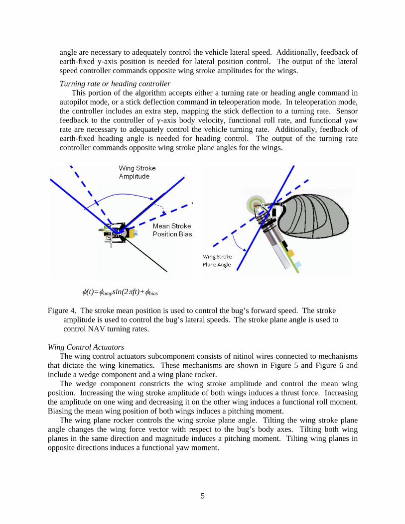
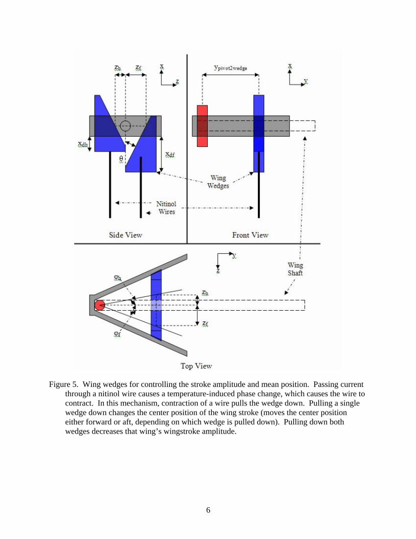
The wing control actuators subcomponent consists of nitinol wires connected to mechanisms that dictate the wing kinematics. These mechanisms are shown in Figure 5 and Figure 6 and include a wedge component and a wing plane rocker.

The wedge component constricts the wing stroke amplitude and control the mean wing position. Increasing the wing stroke amplitude of both wings induces a thrust force. Increasing the amplitude on one wing and decreasing it on the other wing induces a functional roll moment. Biasing the mean wing position of both wings induces a pitching moment.

The wing plane rocker controls the wing stroke plane angle. Tilting the wing stroke plane angle changes the wing force vector with respect to the bug’s body axes. Tilting both wing planes in the same direction and magnitude induces a pitching moment. Tilting wing planes in opposite directions induces a functional yaw moment.

6

Figure 5. Wing wedges for controlling the stroke amplitude and mean position. Passing current through a nitinol wire causes a temperature-induced phase change, which causes the wire to contract. In this mechanism, contraction of a wire pulls the wedge down. Pulling a single wedge down changes the center position of the wing stroke (moves the center position either forward or aft, depending on which wedge is pulled down). Pulling down both wedges decreases that wing’s wingstroke amplitude.

7

(a)

(b)

(c)

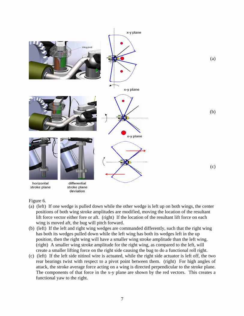
Figure 6. (a) (left) If one wedge is pulled down while the other wedge is left up on both wings, the center

positions of both wing stroke amplitudes are modified, moving the location of the resultant lift force vector either fore or aft. (right) If the location of the resultant lift force on each wing is moved aft, the bug will pitch forward.

(b) (left) If the left and right wing wedges are commanded differently, such that the right wing has both its wedges pulled down while the left wing has both its wedges left in the up position, then the right wing will have a smaller wing stroke amplitude than the left wing. (right) A smaller wing stroke amplitude for the right wing, as compared to the left, will create a smaller lifting force on the right side causing the bug to do a functional roll right.

(c) (left) If the left side nitinol wire is actuated, while the right side actuator is left off, the two rear bearings twist with respect to a pivot point between them. (right) For high angles of attack, the stroke average force acting on a wing is directed perpendicular to the stroke plane. The components of that force in the x-y plane are shown by the red vectors. This creates a functional yaw to the right.

8

NAV MODEL

During the design stage of the control algorithms for the NAV, a mathematical model of the vehicle dynamics was derived. For the NAV, the model employed is the six degree of freedom equations for a rigid body denoted in general form [1] as:

( )

( ) 000

0~

0~

000

mvrt

vGrmII

fGrGrvrt

vm

rrrr

rrr&r

rrrrr&rrrv

=

×+

∂

∂×+×+

=

××+×+×+

∂

∂

ωωωω

ωωωω

where v0 = [u v w]T, ω = [p q r]T, rG = [xG yG zG]T, I0 is the inertia tensor at the origin of the body-fixed frame, f0 = [X Y Z]T, and m0 = [K M N]T.

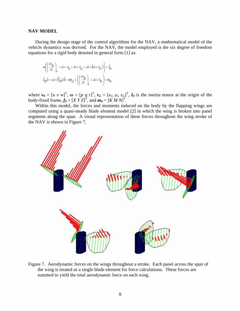
Within this model, the forces and moments induced on the body by the flapping wings are computed using a quasi-steady blade element model [2] in which the wing is broken into panel segments along the span. A visual representation of these forces throughout the wing stroke of the NAV is shown in Figure 7.

Figure 7. Aerodynamic forces on the wings throughout a stroke. Each panel across the span of the wing is treated as a single blade element for force calculations. These forces are summed to yield the total aerodynamic force on each wing.

9

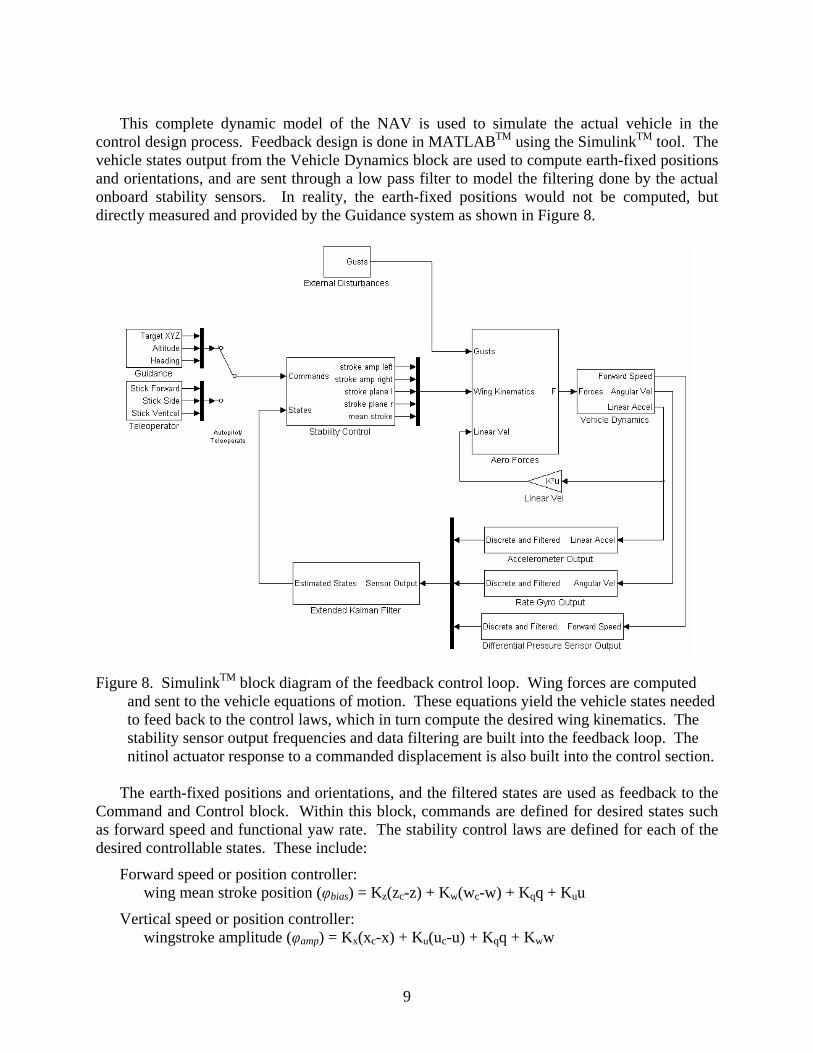
This complete dynamic model of the NAV is used to simulate the actual vehicle in the

control design process. Feedback design is done in MATLABTM using the SimulinkTM tool. The vehicle states output from the Vehicle Dynamics block are used to compute earth-fixed positions and orientations, and are sent through a low pass filter to model the filtering done by the actual onboard stability sensors. In reality, the earth-fixed positions would not be computed, but directly measured and provided by the Guidance system as shown in Figure 8.

Figure 8. SimulinkTM block diagram of the feedback control loop. Wing forces are computed and sent to the vehicle equations of motion. These equations yield the vehicle states needed to feed back to the control laws, which in turn compute the desired wing kinematics. The stability sensor output frequencies and data filtering are built into the feedback loop. The nitinol actuator response to a commanded displacement is also built into the control section.

The earth-fixed positions and orientations, and the filtered states are used as feedback to the

Command and Control block. Within this block, commands are defined for desired states such as forward speed and functional yaw rate. The stability control laws are defined for each of the desired controllable states. These include:

Forward speed or position controller: wing mean stroke position (φbias) = Kz(zc-z) + Kw(wc-w) + Kqq + Kuu

Vertical speed or position controller: wingstroke amplitude (φamp) = Kx(xc-x) + Ku(uc-u) + Kqq + Kww

10

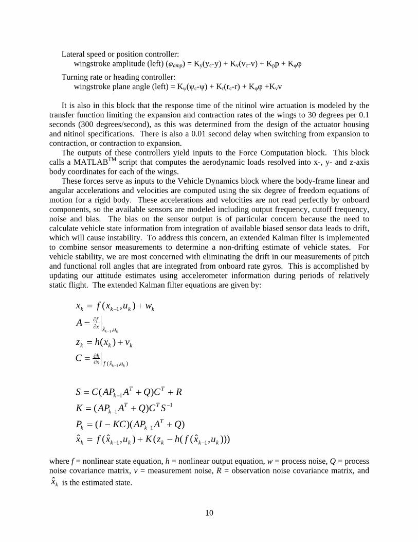
Lateral speed or position controller: wingstroke amplitude (left) (φamp) = Ky(yc-y) + Kv(vc-v) + Kpp + Kφφ

Turning rate or heading controller: wingstroke plane angle (left) = Kψ(ψc-ψ) + Kr(rc-r) + Kφφ +Kvv

It is also in this block that the response time of the nitinol wire actuation is modeled by the

transfer function limiting the expansion and contraction rates of the wings to 30 degrees per 0.1 seconds (300 degrees/second), as this was determined from the design of the actuator housing and nitinol specifications. There is also a 0.01 second delay when switching from expansion to contraction, or contraction to expansion.

The outputs of these controllers yield inputs to the Force Computation block. This block calls a MATLABTM script that computes the aerodynamic loads resolved into x-, y- and z-axis body coordinates for each of the wings.

These forces serve as inputs to the Vehicle Dynamics block where the body-frame linear and angular accelerations and velocities are computed using the six degree of freedom equations of motion for a rigid body. These accelerations and velocities are not read perfectly by onboard components, so the available sensors are modeled including output frequency, cutoff frequency, noise and bias. The bias on the sensor output is of particular concern because the need to calculate vehicle state information from integration of available biased sensor data leads to drift, which will cause instability. To address this concern, an extended Kalman filter is implemented to combine sensor measurements to determine a non-drifting estimate of vehicle states. For vehicle stability, we are most concerned with eliminating the drift in our measurements of pitch and functional roll angles that are integrated from onboard rate gyros. This is accomplished by updating our attitude estimates using accelerometer information during periods of relatively static flight. The extended Kalman filter equations are given by:

))),ˆ(((),ˆ(ˆ))((

)(

)(

)(

),(

11

1

11

1

),ˆ(

,ˆ

1

1

1

kkkkkk

Tkk

TTk

TTk

uxfxh

kkk

uxxf

kkkk

uxfhzKuxfxQAAPKCIP

SCQAAPK

RCQAAPCS

C

vxhz

A

wuxfx

kk

kk

−−

−

−−

−

∂∂

∂∂

−

−+=

+−=

+=

++=

=

+=

=

+=

−

−

where f = nonlinear state equation, h = nonlinear output equation, w = process noise, Q = process noise covariance matrix, v = measurement noise, R = observation noise covariance matrix, and

kx̂ is the estimated state.

11

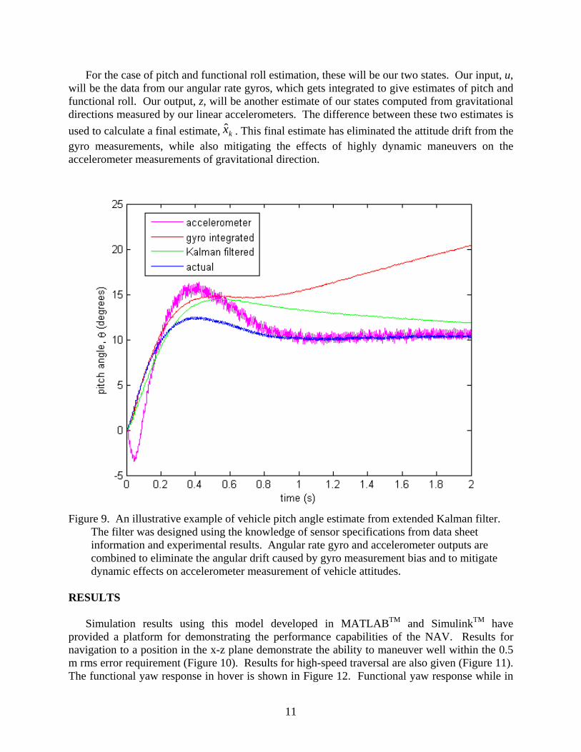
For the case of pitch and functional roll estimation, these will be our two states. Our input, u, will be the data from our angular rate gyros, which gets integrated to give estimates of pitch and functional roll. Our output, z, will be another estimate of our states computed from gravitational directions measured by our linear accelerometers. The difference between these two estimates is used to calculate a final estimate, kx̂ . This final estimate has eliminated the attitude drift from the gyro measurements, while also mitigating the effects of highly dynamic maneuvers on the accelerometer measurements of gravitational direction.

Figure 9. An illustrative example of vehicle pitch angle estimate from extended Kalman filter. The filter was designed using the knowledge of sensor specifications from data sheet information and experimental results. Angular rate gyro and accelerometer outputs are combined to eliminate the angular drift caused by gyro measurement bias and to mitigate dynamic effects on accelerometer measurement of vehicle attitudes.

RESULTS

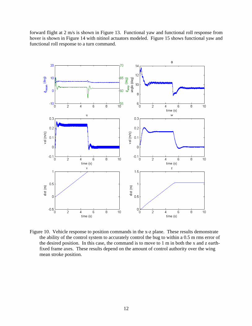
Simulation results using this model developed in MATLABTM and SimulinkTM have

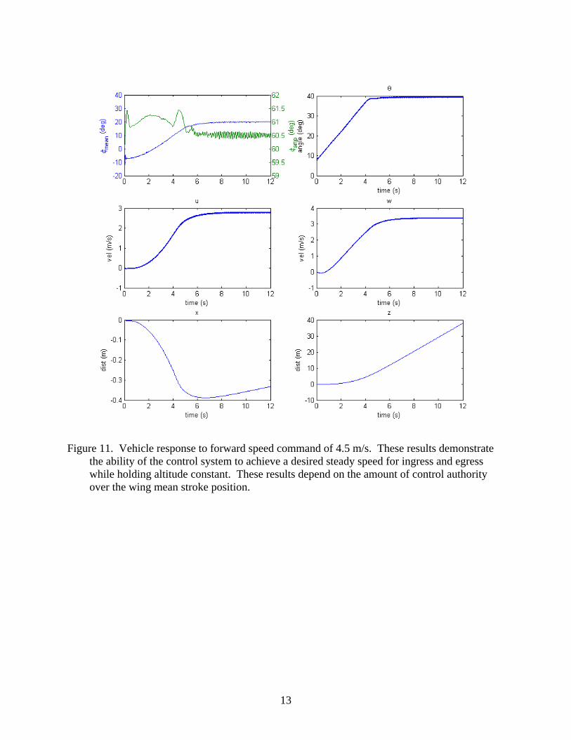
provided a platform for demonstrating the performance capabilities of the NAV. Results for navigation to a position in the x-z plane demonstrate the ability to maneuver well within the 0.5 m rms error requirement (Figure 10). Results for high-speed traversal are also given (Figure 11). The functional yaw response in hover is shown in Figure 12. Functional yaw response while in

12

forward flight at 2 m/s is shown in Figure 13. Functional yaw and functional roll response from hover is shown in Figure 14 with nitinol actuators modeled. Figure 15 shows functional yaw and functional roll response to a turn command.

Figure 10. Vehicle response to position commands in the x-z plane. These results demonstrate the ability of the control system to accurately control the bug to within a 0.5 m rms error of the desired position. In this case, the command is to move to 1 m in both the x and z earth-fixed frame axes. These results depend on the amount of control authority over the wing mean stroke position.

13

Figure 11. Vehicle response to forward speed command of 4.5 m/s. These results demonstrate the ability of the control system to achieve a desired steady speed for ingress and egress while holding altitude constant. These results depend on the amount of control authority over the wing mean stroke position.

14

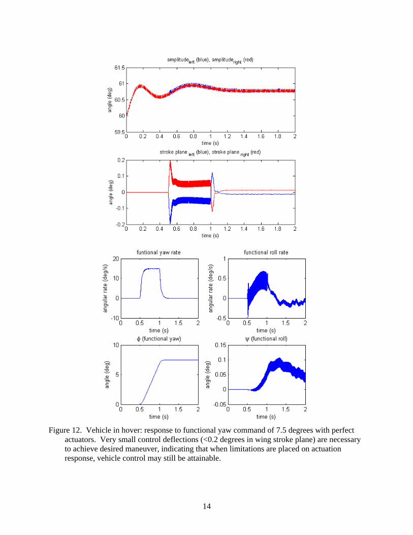
Figure 12. Vehicle in hover: response to functional yaw command of 7.5 degrees with perfect

actuators. Very small control deflections (<0.2 degrees in wing stroke plane) are necessary to achieve desired maneuver, indicating that when limitations are placed on actuation response, vehicle control may still be attainable.

15

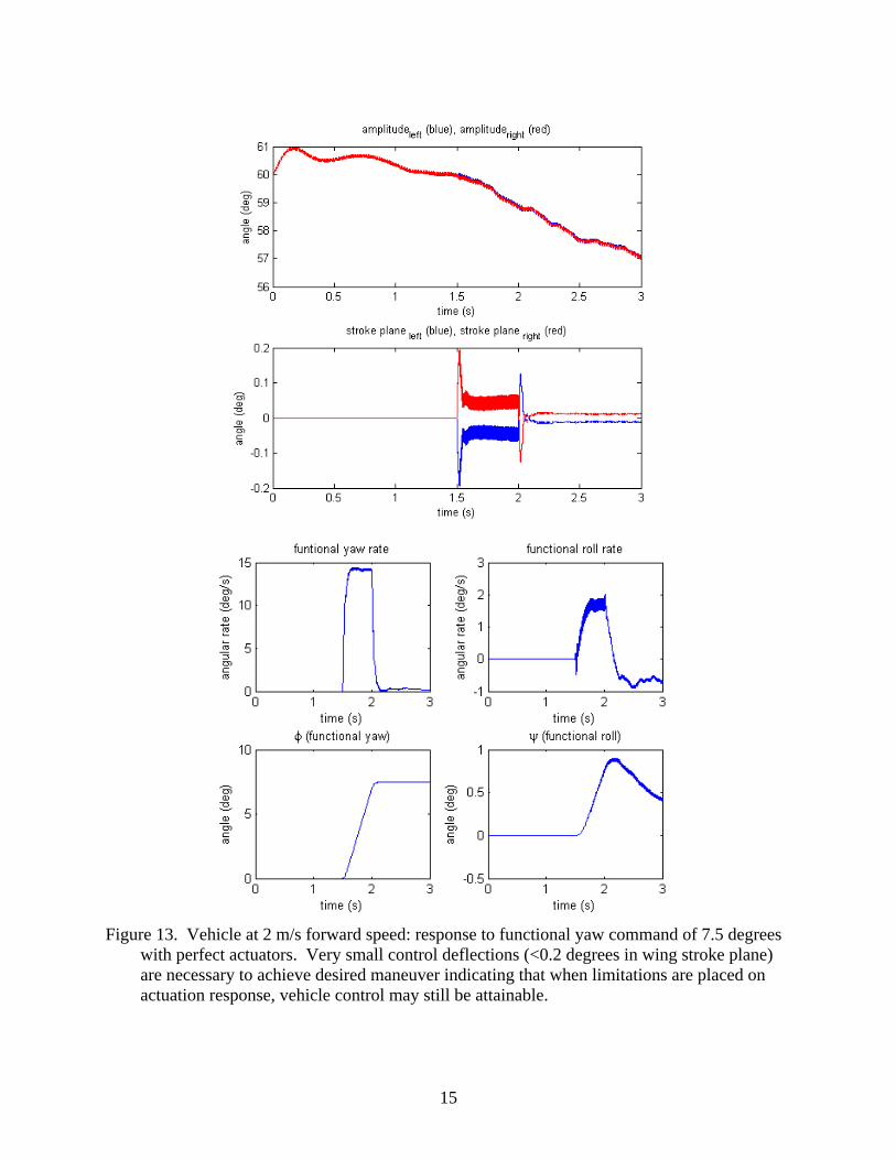
Figure 13. Vehicle at 2 m/s forward speed: response to functional yaw command of 7.5 degrees

with perfect actuators. Very small control deflections (<0.2 degrees in wing stroke plane) are necessary to achieve desired maneuver indicating that when limitations are placed on actuation response, vehicle control may still be attainable.

16

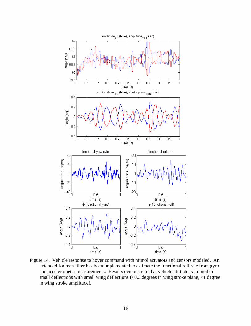
Figure 14. Vehicle response to hover command with nitinol actuators and sensors modeled. An

extended Kalman filter has been implemented to estimate the functional roll rate from gyro and accelerometer measurements. Results demonstrate that vehicle attitude is limited to small deflections with small wing deflections (<0.3 degrees in wing stroke plane, <1 degree in wing stroke amplitude).

17

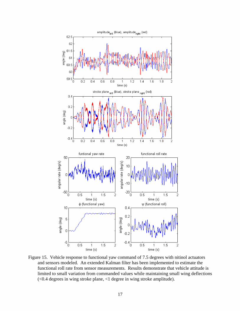
Figure 15. Vehicle response to functional yaw command of 7.5 degrees with nitinol actuators

and sensors modeled. An extended Kalman filter has been implemented to estimate the functional roll rate from sensor measurements. Results demonstrate that vehicle attitude is limited to small variation from commanded values while maintaining small wing deflections (<0.4 degrees in wing stroke plane, <1 degree in wing stroke amplitude).

18

DISCUSSION

The results presented in the paper demonstrate capabilities of a small flapping wing vehicle that provide the basis for maneuvering in confined spaces and countering gusts. The ability to accelerate, stop and turn in seconds or fractions of a second are essential to completing missions in urban environments. Furthermore, the thrust capability enabling high forward speeds produces not only lower travel times, but also an indication that higher wind gusts can be withstood.

The sensors and actuators used on the vehicle have proven adequate for stability control despite their extremely light weight. The effects of sensor drift are mitigated using an extended Kalman filter, as shown in the simulation results.

While the results of this study are promising, there are many modeling and performance aspects that can and should be improved upon. On the modeling side, more detailed models of the actuator mechanisms should be created and implemented. Also, a few inconsistencies were found in the vehicle model that should be corrected including wing placement and orientation, and center of mass location. Future work will focus on improving the performance by increasing maximum forward flight speed and improving turning rates. ACKNOWLEDGMENTS

The Defense Science Office at DARPA was the sponsoring office for this program. Dr. Anita Flynn of MicroPropulsion, Inc. was the primary investigator for the work presented in this paper, and collaboration with her as well as the other team members was invaluable. Members on this project who had specific impact on the controls work included Dr. Will Dickson from the California Institute of Technology, Dr. Rob Playter and his team from Boston Dynamics, Mr. Ankur Mehta from the University of California at Berkeley, Mr. Peter von Behrens of Alternative Motion Solutions, Dr. Ravi Ramamurti of the Naval Research Laboratory, and Dr. William Sandberg of Science Applications International Corporation. REFERENCES [1] T. I. Fossen, Guidance and Control of Ocean Vehicles: John Wiley & Sons, 1994. [2] W. Dickson, A. D. Straw, C. Poelma, and M. Dickinson, "An Integrative Model of Insect

Flight Control," Proceedings of the 44th AIAA Aerospace Sciences Meeting and Exhibit, 2006.