on view processing for a native xml dbms · views than to require a user to comprehend the ......
TRANSCRIPT

ON VIEW PROCESSING FOR A
NATIVE XML DBMS
CHEN TING
NATIONAL UNIVERSITY OF SINGAPORE
2004

Contents
1 Introduction 1
2 Background 8
2.1 XML data model . . . . . . . . . . . . . . . . . . . . . . . . . . 9
2.2 ORA-SS . . . . . . . . . . . . . . . . . . . . . . . . . . . . . . . 10
3 Review of the State of the Art 15
3.1 XML Schema Formats and Graphical view definitions . . . . . . 15
3.2 XML document storage schemes and Native XML DBMS . . . . 17
3.3 XML View Processing techniques . . . . . . . . . . . . . . . . . 21
4 ORA-SS as XML View Definition Format 26
4.1 Why ORA-SS ? . . . . . . . . . . . . . . . . . . . . . . . . . . . 26
4.2 Semantics of ORA-SS views . . . . . . . . . . . . . . . . . . . . 32
i

CONTENTS ii
4.3 Comparison and Summary . . . . . . . . . . . . . . . . . . . . . 35
5 XML Document Storage in Native XML DBMSs 37
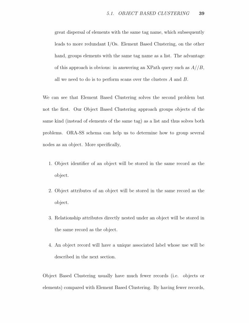
5.1 Object Based Clustering . . . . . . . . . . . . . . . . . . . . . . 38
5.2 Object Labelling Scheme . . . . . . . . . . . . . . . . . . . . . . 40
5.3 Object Based Clustering vs. Element Based Clustering . . . . . 41
6 ORA-SS View Processing on a native XML DBMS 45
6.1 Associative Join: A Primitive XML Join Technique . . . . . . . 46
6.1.1 Structural Query and Associative Query . . . . . . . . . 46
6.1.2 Processing of Associative Query . . . . . . . . . . . . . . 48
6.2 Processing XML views defined in ORA-SS formats . . . . . . . 54
6.2.1 Value Join vs. Associative Join . . . . . . . . . . . . . . 55
6.2.2 The importance of relationship set in ORASS view schema 58
6.2.3 ORA-SS View Transformation Algorithm . . . . . . . . . 59
7 Experiments 64
7.1 XBase description . . . . . . . . . . . . . . . . . . . . . . . . . . 64
7.1.1 ORA-SS Schema Parser . . . . . . . . . . . . . . . . . . 66

CONTENTS iii
7.1.2 Storage Manager . . . . . . . . . . . . . . . . . . . . . . 66
7.1.3 ORA-SS View Transformer . . . . . . . . . . . . . . . . . 69
7.2 Datasets . . . . . . . . . . . . . . . . . . . . . . . . . . . . . . . 69
7.2.1 DBLP Bibliography Record (DBLP) . . . . . . . . . . . 69
7.2.2 Project-Researcher-Paper (JRP) . . . . . . . . . . . . . . 69
7.3 Performances and Analysis . . . . . . . . . . . . . . . . . . . . . 71
7.3.1 The advantages of OBC storage . . . . . . . . . . . . . . 71
7.3.2 View Processing in XBase . . . . . . . . . . . . . . . . . 74
8 Conclusion 82
A Appendix 89
A.1 XSLT Script for view schema in Figure 7.9c: . . . . . . . . . . . 89
A.2 XSLT Script for view schema in Figure 7.9d: . . . . . . . . . . . 90
Chapter 1
Introduction
Traditionally, view is an important aspect of data processing. View support
is desirable because it provides automatic security for hidden data and allows
the same data to be seen by different users in different ways at the same
time. Compared with views in relational database, views for hierarchical data
like XML not only allow basic operations like selection, projection and join,
but also structural swapping of nodes in document trees. For example, a
bibliography XML file (e.g DBLP[19]) contains a list of publications; “under”
each publication there are the authors together with various other properties
of the publication. A frequent view operation on XML data like DBLP is to
find all authors together with their publications, which is indeed a swapping
operation on nodes “Publication” and “Author”.
The starting point of XML view transform is view definition. There are two
1
Chapter 1. Introduction 2
general approaches to define views on source XML data:
1. One way is to define views or queries in script languages like XQuery[32]
or XSLT[33].
2. The alternative approach is to define views by view schemas. Systems
like Clio[24] , eXeclon[11] and the work in [7] fall into this category. Users
only need define a view schema over source data to obtain desired the
view result. This approach is declarative and alleviates user from writing
complex scripts to perform view transformation.
There are problems with the above two approaches which hinder them to
become ideal XML view definition formats.
The query languages (e.g. XSLT and XQuery) cited above in the first approach
usually use regular expressions to express possible variations in the structure of
the data. But the use of regular expression queries means the user is responsible
to phrase their queries in a way that will cover the variations in the structure of
the source data. As an example, suppose again we want to find the information
of authors of each publication; however it is possible that the information we
want may be presented in the source data in two ways: in some places author
is nested under publication (e.g. in a bibliography record) whereas in some
other places publication is nested under author (e.g. in a publication list of
a researcher). Using regular expression means that we have to specify two
patterns: author//publication and publication//author to obtain all relevant
Chapter 1. Introduction 3
information. It would be clear that we can extend the example such that in
the worst case an exponential number of regular expressions need to be written
to cover all possible variation in source data.
To overcome the above problem, a solution is to utilize the ontology of source
data, which consists of the list of tag names of elements and attributes in
the data. Apparently, it is much easier to start from the ontology to define
views than to require a user to comprehend the structural details of source
data. As an example, we can extract two keywords author and publication
from source schema. Next we let author be the parent node of publication
in a view schema meaning that we want to find all matching pairs of author
and publication elements which lie on the same path in source documents and
construct the results by placing publication elements under author elements.
Note that we do not restrict the hierarchical order of elements in a matching
pair in source document. The approach discussed in this thesis greatly extends
the above idea: it allows a user to extract element names from the ontology of
source data and define the structure of view via a view schema. All the tedious
work of finding structural variations of view schemas in the source document
will be left to the view processing back-end system. Thus view definitions can
be phrased succinctly based only on the ontology.
Meanwhile, simple tree/graph-structure schema languages like DTD and XML
Schema used in the second approach for XML view (target) schema can not
express many useful semantics and consequently causes ambiguity. To see this,
Chapter 1. Introduction 4
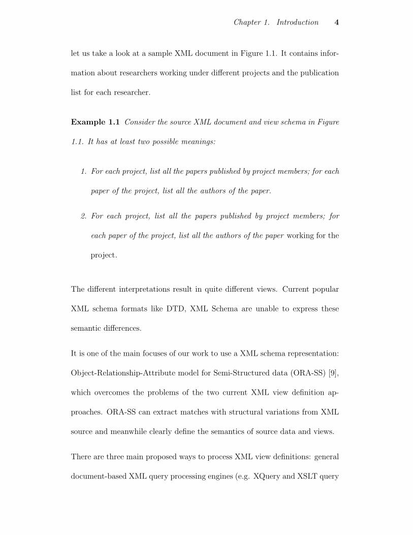
let us take a look at a sample XML document in Figure 1.1. It contains infor-
mation about researchers working under different projects and the publication
list for each researcher.
Example 1.1 Consider the source XML document and view schema in Figure
1.1. It has at least two possible meanings:
1. For each project, list all the papers published by project members; for each
paper of the project, list all the authors of the paper.
2. For each project, list all the papers published by project members; for
each paper of the project, list all the authors of the paper working for the
project.
The different interpretations result in quite different views. Current popular
XML schema formats like DTD, XML Schema are unable to express these
semantic differences.
It is one of the main focuses of our work to use a XML schema representation:
Object-Relationship-Attribute model for Semi-Structured data (ORA-SS) [9],
which overcomes the problems of the two current XML view definition ap-
proaches. ORA-SS can extract matches with structural variations from XML
source and meanwhile clearly define the semantics of source data and views.
There are three main proposed ways to process XML view definitions: general
document-based XML query processing engines (e.g. XQuery and XSLT query

Chapter 1. Introduction 5
< root > . Root< Project J Name = ”j1” > . Project
< Researcher R Name = ”r1” > ¦ J Name< Paper P Name = ”p1”/ > . Researcher
< /Researcher > ¦R Name< Researcher R Name = ”r2” > . Paper
< Paper P Name = ”p1”/ > ¦P Name< Paper P Name = ”p2”/ > (b) Source Schema
< /Researcher >< Project J Name = ”j2” > . Root
< Researcher R Name = ”r2” > . Project< Paper P Name = ”p1”/ > ¦J Name< Paper P Name = ”p2”/ > . Paper
< /Researcher > ¦P Name< Researcher R Name = ”r3” > .Researcher
< Paper P Name = ”p2”/ > ¦R Name< /Researcher > (c) View Schema
< /Project >< /root >(a) Source XML document
Figure 1.1: An sample XML document with DTD-like source andview schemas
engines such as Xalan[30],XT[8],SAXON[26] and Quip[25]) traverse in-memory
source data trees to output the result tree. Another possible solution is to load
the XML data file into a relational or object-relational database and perform
view transformation using available RDBMS facilities. This method requires
conversion from hierarchical data and schema to relational data and schema.
The third approach and also the one used in this paper is to use a native
XML DBMS to support view transformation. A native XML DBMS is one
which is designed and implemented from the ground up for storage and query
processing of XML data.
Recently, great efforts have been put into the study of XML query optimiza-
tion. Techniques[1][3][34] are developed mainly for processing of queries de-

Chapter 1. Introduction 6
fined in the XPath[31] standard, which can express both path and branch
patterns. However, as we demonstrated earlier, XML views defined based on
the ontology of source data can not be mapped to a single XPath expres-
sion. To meet the new challenges, we investigate new XML query processing
techniques for views defined via schema mapping. The new techniques are
integrated with our native XML DBMS XBase to process XML views defined
in ORA-SS format. Experiment results demonstrate the advantages of our
method over current state-of-the-art approaches.
The main contributions of our work are:
1. We introduce a new view schema definition format based on ORA-SS
which can
(a) Extract matches with structural variants in tree-structured data like
XML without issuing an excessive number of queries as XSLT and
XQuery do.
(b) Express a large variety of semantics which results in different view
which is not possible under view schema format like DTD and XML
Schema.
2. A native XML document storage and view transformation prototype
XBase which implements novel XML document storage scheme and query
processing techniques to obtain views defined in our view schema format.

Chapter 1. Introduction 7
This thesis is organized as follows:
• Chapter 2 introduces XML data model and the conceptual XML data
model ORA-SS used in our work.
• Chapter 3 surveys recent work on graphical XML view definition, native
XML DBMSs and the latest XML query/view processing techniques.
• Chapter 4 explains in details the advantages of using the ORA-SS data
model for XML view schema definition.
• Chapter 5 explains storing XML documents in a new Object Based Clus-
tering scheme in our prototype XML DBMS system: XBase.
• Chapter 6 shows a new XML query processing technique: Associative
Join to efficiently process XML views defined in ORA-SS format.
• Chapter 7 shows a series of experiments to test the performances of view
transformations in our XML DBMS: XBase.
• Chapter 8 concludes the thesis.

Chapter 2
Background
Recently there has been an increased interest in managing data that does
not conform to traditional data models. The driving factors behind the shift
are diverse: data coming from heterogeneous sources(especially the Web) may
not conform to the traditional Relational or Object oriented model physically;
meanwhile missing attributes and frequent updates to both data and schema
render traditional data models inappropriate in the logical level. The term
semi-structured data has been coined to refer to data with the afore-mentioned
nature. In particular, XML is emerging as one of the leading formats for
representing semi-structured data.
In this chapter, we first briefly describe the XML data model. Next we intro-
duce a recently proposed conceptual model for XML data: Object Relationship
Attribute Model for Semistructured Data or ORA-SS.
8

2.1. XML DATA MODEL 9
2.1 XML data model
An XML document is generally presented by a labelled directed graph G =
(VG, EG, rootG,∑
G). Each node in the vertex set VG is uniquely identified by
its oid. A node can be of the following types: Element, Attribute, Content.
Each node also has a string-literal label from the alphabet∑
G. The root
node is denoted by rootG. There are two types of edges in the edge set EG.
The tree edges represent parent-child relationships between two nodes in VG.
Note that any node except rootG has one and only one incoming tree edge but
any number of outgoing tree edges. The reference edges represent reference
relationships defined using ID/IDREF features in XML. As an example, the
following XML element student has an id attribute whose value is unique in
the entire document:
< student id = “U888” name = “Tim Duncan” age = “27” >
Another element can refer to the above element using an ref attribute whose
value is equal to the id value of referred element. E.g:
< student ref = “U0202888” >
The advantage to use ID/IDREF is that we can avoid replications of data in
XML documents.

2.2. ORA-SS 10
If we consider only tree edges, an XML document can be viewed as a tree.
In the remaining of this paper, we focus on tree-structured XML data model
which doesn’t include ID/IDREF edges.
2.2 ORA-SS
DTD and XML Schema are de facto schema formats for XML documents, why
do we need yet another model? There are multiple reasons. First of all, DTD
and XML Schema are text-based; they are primarily designed for validation of
XML documents. In the domain of view definition, it is troublesome to define
views in DTD and XML Schema directly. On the other hand, graphical and
conceptual data models are much more intuitive and easy to design. Next and
more importantly DTD and XML Schema provide little features for expressing
semantic constraints over data they represent as we have pointed out in the
introduction section.
We introduce a semantically expressive data model ORA-SS[9]. ORA-SS has
two important types of diagrams. An ORA-SS instance diagram represents a
XML document while an ORA-SS schema diagram models the corresponding
schema. Drawing from the success of Entity-Relationship model, an ORA-SS
schema diagram has the following basic concepts:
1. Object Class

2.2. ORA-SS 11
Object classes are similar to entity types in the Entity-Relationship model.
Object classes are represented as rectangles in ORA-SS Schema diagram.
2. Relationship Type
Two or more object classes are connected via a relationship type in
schema diagram. Labels associated with edges between object classes
denote the relationship type names and their degrees.
3. Attribute
Attributes are properties of an object class or a relationship type. At-
tributes are represented as circles in ORA-SS Schema diagrams. An
attribute can also be the identifier of an object instance and is repre-
sented as a solid circle in ORA-SS schema diagrams. Labels associated
with edges between object classes and attributes indicate which relation-
ship type the attribute belongs to. Edges between object classes and
attributes without labels indicate the attributes are properties of the
object classes.
In ORA-SS instance diagrams, objects are represented as rectangles labelled
with class names. Labels under leaf nodes show attribute names followed by
their values.
The most important difference between ORA-SS and DTD/XML Schema is
that for each object class, an ORA-SS schema indicates which relationship

2.2. ORA-SS 12
types it participates in. Similarly for each attribute, an ORA-SS schema ex-
plicitly indicates its owner object class or relationship type. This information
can be obtained from labels on edges in an ORA-SS schema diagram. In gen-
eral, an edge with a relationship type label of degree n (n ≥ 2) indicates that
the two object classes (say A , B and A is B’s parent) linked by the edge and
the n− 2 closest ancestors of A form a n-ary relationship type.
Example 2.1 Fig. 2.1 shows an ORA-SS instance diagram and and Fig. 2.2
shows the corresponding schema diagram for the XML file in Fig. 1.1a (with
a few additional attributes on Position and Date).
Like DTD, XML Schema and Data-Guide[12], an ORA-SS schema diagram
shows the tree structure of the XML file. What’s more, the ORA-SS schema
diagram explicitly indicates the following facts about XML documents conform-
ing to the schema:
1. There are two binary relationship types in the schema: Project−Researcher
(JR) and Researcher − Paper (RP). A project can have several re-
searchers and a researcher can work in different projects. Meanwhile,
the set of papers under a researcher doesn’t depend on the project he/she
works in.
2. Position is an attribute of relationship type JR instead of Researcher.
This means that a researcher may hold different positions across projects
he works in.
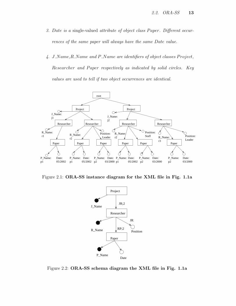
2.2. ORA-SS 13
3. Date is a single-valued attribute of object class Paper. Different occur-
rences of the same paper will always have the same Date value.
4. J Name,R Name and P Name are identifiers of object classes Project,
Researcher and Paper respectively as indicated by solid circles. Key
values are used to tell if two object occurrences are identical.
r2
Position: Leader
Paper
P_Name:p1
Date:05/2002
P_Name:p1
Date:
Paper Paper
Researcher
R_Name:
root
Project Project
J_Name:j1
Researcher Researcher
R_Name:r1
Researcher
P_Name:p1
Date:05/2002
P_Name:p2
Date:03/2000
P_Name:p2
Date:03/2000
R_Name:r3
03/2000
Paper Paper Paper
J_Name:j2
R_Name:r2
Position:Staff Position:
Leader
P_Name: Date:05/2002 p2
Figure 2.1: ORA-SS instance diagram for the XML file in Fig. 1.1a
RP;2
JR
JR;2
Position
DateP_Name
R_Name
J_Name
Paper
Researcher
Project
��������������������
��������������������
������������
������������
��������������������
��������������������
������������
������������
���������
���������
����
����
����
Figure 2.2: ORA-SS schema diagram the XML file in Fig. 1.1a

2.2. ORA-SS 14
Information about relationship types in an ORA-SS schema can be obtained
through several possible ways:
1. In the case that the XML document examined is exported from a re-
lational source, then by knowing operations performed on the source
tables to generate the XML data, we can deduce the ORA-SS schema.
For example, in the above example, if we know that the XML file are
generated by joining two relational tables (Project, Researcher) and
(Researcher, Paper), then we can easily know there are two binary re-
lationship types in the ORA-SS schema.
2. In the case that we only have XML documents, then we need to solve
the classic schema discovery problem. This thesis does not focus on the
problem of ORA-SS schema discovery; we use the example to illustrate
the intuition. It should be noted that the relationship type information
implies data dependencies. First we need to assign keys for each object
class to tell if two objects are the same. Next if we find that all occur-
rences of the same Researcher object have the same set of papers as
their children, then Researcher and Paper may probably form a binary
relationship type. This fact has to be confirmed by users because the file
may be too small to find an exception. Otherwise it means the set of pa-
pers under a researcher depends also on the project the researcher works
in; then Project, Researcher and Paper forms a ternary relationship.

Chapter 3
Review of the State of the Art
In this chapter, we review topics related to XML views and view processing.
First we survey popular XML schema formats and query languages and the
relatively new field on graphical XML query language. Next we study XML
document storage schemes which have direct impact on XML view processing.
Finally we review state-of-the-art XML query processing techniques.
3.1 XML Schema Formats and Graphical view
definitions
DTD[10] and XML Schema[27] are current dominant XML schema standards.
DTD is essentially an extension of context-free grammar (CFG) which is able
to specify graph structures of XML data as well as various constructs like
15

3.1. XML SCHEMA FORMATS AND GRAPHICAL VIEW DEFINITIONS 16
Element, Attribute and ID/IDREF . XML Schema has many more features
compared with DTD. It allows the definition of complex data types in a schema
which is not present in DTD. XML Schema also has features like inheritance.
XML Schema is gradually replacing DTD as the standard XML schema format.
Under the W3C, there are two competing XML query language standards:
XQuery[32] and XSLT[33]. While it is a matter of taste to say which is better,
it seems that XQuery is gaining the upper-hand because strong endowment
from the database research community. Both XQuery and XSLT provide rich
features as query languages and thus become complex. Both of them follow
the SQL tradition and use For-Let-Where-Return as the basic query skeleton.
Aggregate functions are also supported by both languages. It should be noted
that XPath[31] is used to extract information from XML documents in both
standards.
One of the classical graphical query languages is Query By Example (QBE)
from IBM. A graphical query language is often preferred over text-based query
language because of its intuitiveness and ease of use. In the context of XML
graphical query language, important recent developments include XML-GL[2]
and GLASS[23]. XML-GL is built on the base of a graphical representation
of XML documents and DTDs, which is called XML graphs. An XML graph
represents the XML documents and DTDs by means of labelled graphs. An
XML-GL query consists of two parts: left hand side (LHS) and right hand side
(RHS). The LHS of an XML-GL query indicates the data source and conditions

3.2. XML DOCUMENT STORAGE SCHEMES AND NATIVE XML DBMS 17
and the RHS constructs the output. Compared with XML-GL, GLASS is
a more expressive XML visual query language. It employs ORA-SS as its
XML data model. GLASS also supports negation, quantifier and conditional
output, which are not present in XML-GL. A GLASS query consists of LHS
and RHS parts just as XML-GL; however, it has an optional Conditional Logic
Window (CLW) which allows specification of many useful logic conditions such
as negation, existential constraints and IF-THEN conditions.
Example 3.1 The GLASS query in Figure 3.1 displays the members with their
names who have written a publication titled “Introduction to XML or “Intro-
duction to Internet; and for those members who have written Introduction to
XML, it also displays all information about the projects that they have partic-
ipated in.
The vertical line separates LHS and RHS of the GLASS query. : A : and
: B : are conditions which require the members should have a publication titled
“Introduction to XML ( or “Introduction to Internet) respectively.
3.2 XML document storage schemes and Na-
tive XML DBMS
The storage scheme has a great impact on the performance of native XML
DBMS systems. Several native storage schemes have been proposed to store

3.2. XML DOCUMENT STORAGE SCHEMES AND NATIVE XML DBMS 18
Figure 3.1: An example of GLASS query
XML documents:
1. Element-Based scheme (EB). In EB scheme (Figure 3.2b), each element
(and attribute which is also treated as an “element”) is an atomic unit
of storage and elements in an XML document are stored according to
their document (i.e. pre-order) order. The Lore system[21] is a classical
example which uses EB scheme.
2. Element-Based Clustering scheme (EBC). In EBC scheme (Figure 3.2c),
elements with the same tag name are first clustered together and in each
cluster elements are listed by their document order. TIMBER[14] is a
native XML DBMS using EBC scheme.
3. Subtree-based scheme (SB). In SB scheme (Figure 3.2d), a XML docu-
ment tree is divided into subtrees according to the physical page size,
following the rule that the size of a subtree should be as close as possible
to the size of the physical page. A split matrix is defined to make certain
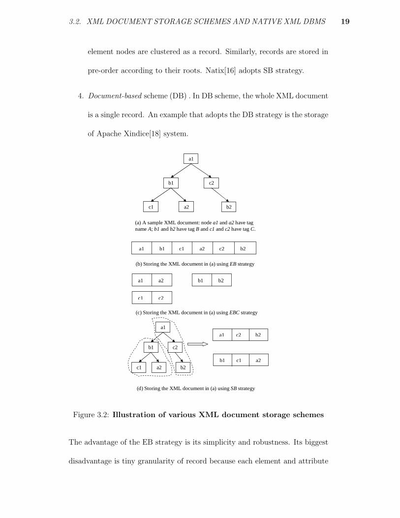
3.2. XML DOCUMENT STORAGE SCHEMES AND NATIVE XML DBMS 19
element nodes are clustered as a record. Similarly, records are stored in
pre-order according to their roots. Natix[16] adopts SB strategy.
4. Document-based scheme (DB) . In DB scheme, the whole XML document
is a single record. An example that adopts the DB strategy is the storage
of Apache Xindice[18] system.
a1
b1 c2
c1 a2 b2
(a) A sample XML document: node a1 and a2 have tag name A; b1 and b2 have tag B and c1 and c2 have tag C.
a1 b1 c1 a2 c2 b2
(b) Storing the XML document in (a) using EB strategy
a1 a2 b1 b2
c1 c2
(c) Storing the XML document in (a) using EBC strategy
a1
b1 c2
c1 a2 b2
a1 c2 b2
b1 c1 a2
(d) Storing the XML document in (a) using SB strategy
Figure 3.2: Illustration of various XML document storage schemes
The advantage of the EB strategy is its simplicity and robustness. Its biggest
disadvantage is tiny granularity of record because each element and attribute

3.2. XML DOCUMENT STORAGE SCHEMES AND NATIVE XML DBMS 20
is treated as an atomic unit of storage. Tiny granularity results in too many
pointers (physical pointer or logical pointer) among records, which leads to
more storage space and increasing the cost of updating. Meanwhile, because
elements with the same tag are not clustered together, the scheme incurs more
I/O costs in processing queries involving only a small number of tags. The main
disadvantage of the SB strategy is its relatively large granularity of record. In
some cases, most data gained by a single page read from disk is useless for query
processing. The DB strategy treats a whole document as a single record. It is
fine with small files but not suitable for large ones. The whole XML document
must be read and be memory-resident during query processing, which requires
too much memory. EBC to some extents, avoids the problems of other storage
schemes and thus is a more popular XML storage option currently.
Besides the choice of storage schemes, native XML DBMSs usually number
node of an XML document for query processing purposes and store these num-
bers together with records in the database. One of these numbering schemes[3]
is to use (DocumentNo, StartPos : EndPos, LevelNum) to number each node
in the XML file. DocumentNo refers to the document identifier. StartPos and
EndPos are calculated by counting the number of element start and end tags
from the document root until the start and the end of the element. LevelNum
is the nesting depth of the element in the data tree.
Node numbering allows fast processing of XML documents because using the
numbering scheme, the calculation to tell if two nodes are of ancestor/descendant

3.3. XML VIEW PROCESSING TECHNIQUES 21
or parent/child relationship is done in constant time. For example, in the num-
bering scheme we introduced previously, node A is a descendant of node B if
and only if StartPos(A) > StartPos(B) and EndPos(A) < EndPos(B). No-
tice that using node numbering scheme, we do not need to travel the edges (note
that in the number of travelling steps is dependant on document height) from A
to B to do the ancestor/descendant testing. Similarly, node A is the parent of
node B if and only if StartPos(A) > StartPos(B), EndPos(A) < EndPos(B)
and LevelNum(A) == LevelNum(B)− 1.
3.3 XML View Processing techniques
Query processing and optimization of graph/tree structured data like XML
poses many new problems. In the context of graph structured XML data,
many techniques to build a structural summary on source XML data have
been proposed. Summary structures of XML data, which play a similar role to
indexes of traditional relational databases, are usually much smaller than the
corresponding source data in size and thus they can be used to answer path
and branch queries efficiently. 1− index[22],A(k)− index[17],D(k)− index[4]
and M(k) − index[13] are recently proposed XML structural summaries to
answer path queries.
We focus on tree-structured XML data in this thesis. In the context of
tree (which is a special kind of graph) structured XML data, more opti-
3.3. XML VIEW PROCESSING TECHNIQUES 22
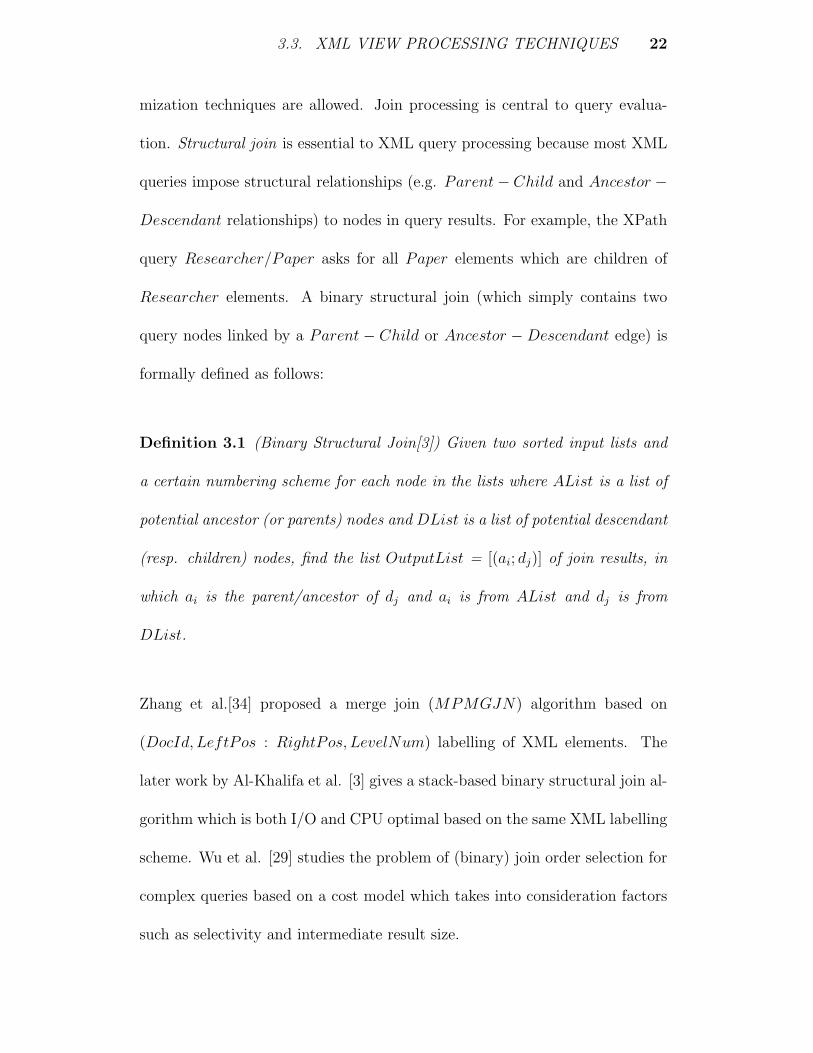
mization techniques are allowed. Join processing is central to query evalua-
tion. Structural join is essential to XML query processing because most XML
queries impose structural relationships (e.g. Parent− Child and Ancestor −
Descendant relationships) to nodes in query results. For example, the XPath
query Researcher/Paper asks for all Paper elements which are children of
Researcher elements. A binary structural join (which simply contains two
query nodes linked by a Parent − Child or Ancestor −Descendant edge) is
formally defined as follows:
Definition 3.1 (Binary Structural Join[3]) Given two sorted input lists and
a certain numbering scheme for each node in the lists where AList is a list of
potential ancestor (or parents) nodes and DList is a list of potential descendant
(resp. children) nodes, find the list OutputList = [(ai; dj)] of join results, in
which ai is the parent/ancestor of dj and ai is from AList and dj is from
DList.
Zhang et al.[34] proposed a merge join (MPMGJN) algorithm based on
(DocId, LeftPos : RightPos, LevelNum) labelling of XML elements. The
later work by Al-Khalifa et al. [3] gives a stack-based binary structural join al-
gorithm which is both I/O and CPU optimal based on the same XML labelling
scheme. Wu et al. [29] studies the problem of (binary) join order selection for
complex queries based on a cost model which takes into consideration factors
such as selectivity and intermediate result size.

3.3. XML VIEW PROCESSING TECHNIQUES 23
A more general form of XML query consists of more than binary relationships.
Formally, a twig pattern query Q is a small tree whose nodes are predicates
(e.g. node type test) and edges are either Parent-Child edges or Ancestor-
Descendant edges. A twig pattern match in a XML database D is a mapping
from nodes in Q to database nodes in D such that:
1. Node predicates in Q are satisfied by the corresponding database nodes;
and
2. The Parent-Child or Ancestor-Descendant relationships between query
nodes are also satisfied by the corresponding database nodes.
Usually, a match to a twig pattern query with n nodes is represented as a
n − ary tuple of databases nodes. For example, the following twig pattern
query written using XPath format
section[/title]/paragraph//figure
selects distinct tuples each of which has 4 elements with types section, title,
paragraph and figure respectively. In addition, in each tuple, the figure
element should be a descendant of the paragraph element which in turn is the
child of the section element which is the parent of the title element.
Formally, the problem of twig pattern matching is defined as:

3.3. XML VIEW PROCESSING TECHNIQUES 24
Definition 3.2 (Twig Pattern Matching [1] )
Given a query twig pattern Q, and an XML database D that has index struc-
tures to identify database nodes that satisfy each of Q’s node predicates, com-
pute ALL the answers to Q in D.
Prior work[29] on XML path pattern processing usually decomposes a twig
pattern into a set of binary relationships which can be either parent-child
or ancestor-descendant relationships. After that, each binary relationship is
processed using binary structural join techniques and the final match results
are obtained by joining individual binary join results together. For example,
the afore-mentioned XPath expression can be processed by a series of struc-
tural joins and merges: (1) structurally join the list of figure with the list
of paragraph to get the paragraphs with at least one figure descendant (2)
structurally join the paragraphs resulted from step 1 with the list of section
(3) structurally join the section list constructed in step 2 with the list of title
(4) finally merge the list of section resulted in step 3 to get the final output.
The intermediate output of each step except the final one is also represented
as a list of tuples. The main problem with the above solution is that it may
generate large and possibly unnecessary intermediate results. For example,
if in the source document there are a lot of paragraph elements with figure
descendants but few of which have section parents, most of the intermediate
output of step (1) becomes redundant once we join it with the list of section

3.3. XML VIEW PROCESSING TECHNIQUES 25
element.
Without resorting to the inefficient traditional decompose-then-join approach,
twig join tries to evaluate branching queries as a whole. In their paper, Bruno
et al. [1] propose a novel holistic method of XML path and twig pattern pro-
cessing based on Element-Based Clustering which avoids storing intermediate
results unless they contribute to the final results. Their algorithm is I/O and
CPU optimal to twig pattern query consisting of only Ancestor-Descendant
edges. Jiang et al.[15] studies the problem of holistic twig joins on all/partly
indexed XML documents. Chen et al. [5] proposes a new XML element clus-
tering approach which can process Ancestor-Descendant only, Parent-Child
only and XML twig patterns with only one branch node optimally.

Chapter 4
ORA-SS as XML View
Definition Format
ORA-SS schema diagrams can be used to define XML views with a great
variety of semantics. In this chapter, we first explain the advantages of ORA-
SS schema over popular tree/graph based XML schema formats likes DTD
and XML Schema in defining XML views. Next, we explain in detail how to
interpret XML view schemas defined in ORA-SS.
4.1 Why ORA-SS ?
The additional information in the ORA-SS schema diagram such as relation-
ship type sets and attribute types allows to define XML views with a great
26

4.1. WHY ORA-SS ? 27
variety of semantics.
Figure 4.1 shows such an interesting example. Although the two view schemas
over source schema in Figure 2.2 look nearly identical from a tree-structure
point of view, they represent quite different semantics:
• Figure 4.1a has two binary relationship types. The intention of the view
schema is to find all the papers published by researchers in a project;
and for each paper to find all of its authors.
• Figure 4.1b has only one ternary relationship type. The view is defined
to find all the papers published by researchers in a project just as Fig-
ure 4.1a; however, for each paper Figure 4.1b only finds those authors
working for the project.
To illustrate the ideas, Figure 4.2 gives “correct” (which we will define formally
in Section 4.2) views for view schemas in Figure 4.1a and b. To simplify the
diagram, we use a variant of ORA-SS instance diagram which use identifiers
to represent an object. Notice that both views are correct but view in Figure
4.1a has two more root-to-leaf paths (here we use XPath-like expressions to
represent paths.) than Figure 4.1b: root/j1/p2/r3 and root/j2/p1/r1. They
do NOT appear in view Figure 4.1b because researcher r3 is the author of
paper p2 but not a member of project j1.
The above example clearly shows the expressive power of ORA-SS schema

4.1. WHY ORA-SS ? 28
diagram. We are going to explain in detail how different semantics are derived
from ORA-SS view schemas in the next section.
R_Name
P_Name
J_Name
PR;2
JP;2
Researcher
Paper
Project
����������������
����������������
����������������
����
����
����
Researcher
Paper
Project
R_Name
JPR;3
P_Name
J_Name
(a) (b)
Figure 4.1: Two view schemas for source schema in Fig. 2.2
j1
r1
j2
r2
p1 p2
root
p2
r2 r3
p1
r2 r2 r3 r1
j1
r1
j2
r2
p1 p2
root
p2
r2 r3
p1
r2 r2
(a) Instance of view schema Fig. 4.1a (b)Instance of view schema Fig. 4.1b
Figure 4.2: Correct views for views schemas in Fig. 4.1
User needs only the ontology of source data to define ORA-SS view schemas;
by doing so we free the user from the trouble of looking into complicated details
of the source schema. In terms of mapping from an ORA-SS source schema
to a user-defined view schema, we extend the work by Chen[6] and define the
following basic operations:
1. Projection Just like projection operations in relational model, projec-

4.1. WHY ORA-SS ? 29
tion in XML context drops object class and/or attributes in the source
schema.
2. Selection The selection operator filters away object instances or attribute
values by applying predicates to object classes or attributes in the source
schema.
3. Swapping XML employs a tree data model; naturally, many views defined
by swapping node positions in the source schema tree. This is an operator
that finds no counter-part in the relational model.
4. Join Two relationship types can be joined on one or more common object
classes.
5. Union Two identical relationship types or object classes can be unioned.
Remark: It should be pointed out that a user do not need to worry about these
mapping operations; however back-end view transformation engines can utilize
these mapping information for optimization.
Example 4.1 Figure 4.3 defines a schema mapping for view transformation.
The source ORA-SS schema has two branches with four binary relationship
types. The relationship R1 : Project − Researcher lists researchers working
under each project. The relationship R2 : Researcher − Paper shows the
publication lists of each researcher. The relationship R3 : Conference−Paper

4.1. WHY ORA-SS ? 30
root
Project
Researcher
Paper
Conference
Paper
Researcher
root
Project
Paper
Researcher
2
2
Source Schema View Schema
R1;2
R2;2
R3;2
R4;2
Figure 4.3: Source Schema to View Schema Mapping with object class
mapping
lists papers published in each conference and the relationship R4 : Paper −
Researcher records the authors of each paper.
The view schema has only two binary relationship types. The relationship
Project−Paper shows all the papers published by project members of a project.
It is formed by first join R1 and R2 on Researcher and then taking projection
on the join result. The relationship Paper − Researcher shows the complete
author list of each paper. It is constructed by first swapping R2 and then
unioning the resulting relationship with R4.
Figure 4.4 shows a sample XML document conforming to the source ORA-SS
schema in Figure 4.3. The correct view transformation result is shown in Figure
4.5. The concept of object identifier in ORA-SS, which is missing in both DTD

4.1. WHY ORA-SS ? 31
and XML Schema, is essential to correctly swap and merge objects in source
XML documents to construct views. Due to its tree structure, an object with
the same identifier may have several occurrences in the source document. A
swap operation in XML view transformation may result in occurrences of the
same object placed under the same parent and thus should be merged to
reduce redundancy. Without the concept of object identifer, merging object
occurrences is not possible. As an illustration, the relationship type Paper −
Researcher in the view schema of Figure 4.3 swaps the order of R2 in the
source schema. Correspondingly, Paper objects now should be placed above
Researcher objects in the view. Notice that in the sample XML document
in Figure 4.4, there are three occurrences of object p2, using their object
identifers, we can merge them and group their children together in the view.
Certainly we can not obtain the desired view result if DTD or XML Schema
is used as the schema definition format because they do not consider object
identifiers.
j1
r1 r2
p1 p2 r6r3r4r1
p4p1
c1
p4p2p1
r3r1
j2
p2
Figure 4.4: Source XML Document of source schema in Fig. 4.3

4.2. SEMANTICS OF ORA-SS VIEWS 32
j1
p1 p2
r1 r4 r1 r2
j2
p1 p2 p4
r1 r2 r6r1 r4 r3
Figure 4.5: View XML Document of view schema in Fig. 4.3 based
on source XML document in Fig. 4.4
4.2 Semantics of ORA-SS views
ORA-SS, used as the view schema format, introduces different semantics com-
pared to XPath queries. Thus in this section, we define formally the semantics
of ORA-SS view schema.
Our most important assumption is that several objects are related if they are
located on the same path in a source document. Based on this assumption,
given a relationship R: O1/O2/ . . . /On in ORA-SS view schema, a match of
R is a path o1/o2/ . . . /on for which:
1. Object oi is of class Oi.
2. o1, o2, . . . , on should be located on some path p in the source document
but there is no restriction on their order on p.
A relationship type R: O1/O2/ . . . /On in ORA-SS view schema allows much
more possible matches than the XPath expression: O1//O2// . . . //On. The
4.2. SEMANTICS OF ORA-SS VIEWS 33
reason is that the latter not only requires that the n nodes in a match are
located on the same path but also impose the hierarchical ordering on the
objects (i.e. objects from o1 to on should have increasing depths). The seman-
tics of ORA-SS view schema is useful in many practical scenarios and using it
avoids an excessive number of XPath expressions needed to replace equivalent
ORA-SS view schemas as we pointed out in the introduction chapter. We
extend the idea to define ORA-SS view schema semantics.
In general, a view transformation based on schema mappings can be seen as
an assignment from a source document to its view which satisfies various con-
straints imposed by a view schema which will be discussed shortly. Because
view document trees consist of a collection of paths, naturally we should con-
sider defining constraints over these paths. Formally, we define a complete
path in an ORA-SS instance tree to be a path from the root to a leaf ob-
ject. XPath-like expressions are used to represent paths. For example, path p:
o1/o2/ . . . /on denotes a path with object oi as the parent of object oi+1. An
object in the path is denoted by its identifier. A complete path p is said to be
of type P if p is an instance of a root-to-leaf path P in the ORA-SS schema
diagram. Sub-path of a path p is a segment of p. We say a sub-path p′ is a
relationship sub-path if p′ is an instance of relationship type R. A complete
path is formed by the root and one or several relation sub-paths.
For example, in Figure 4.4, the complete path root/j1/r1/p1 consists of rela-
tionship sub-path j1/r1 of type Proj/Researcher and r1/p1 of type Researcher/Paper.

4.2. SEMANTICS OF ORA-SS VIEWS 34
View schemas defined in ORA-SS impose the following constraints on views:
Definition 4.1 (Relationship Constraint) A complete path p is in the view
tree if p is of type P with P being a root-to-leaf path in the view schema and
for each of p’s relationship sub-paths pi : o1/o2/ . . . /on of some relationship
type R on P , o1,o2,. . .,on lie on some path in the source document, possibly in
a different order than they are in pi.
Definition 4.2 (Object Attribute Constraint) A sub-path p: o/a with object o
as the owner object of object attribute a is in the view tree if o/a is also in the
source document.
Definition 4.3 (Relationship Attribute Constraint) A relationship sub-path
with its relationship attribute a (or p: o1/o2/ . . . /on/a) is in the view tree if a
lies on the same path with o1, o2, . . . , on in the source document. The order of
o1, o2, . . . , on in the source document may be different from their order in p.
A correct view is indeed the collection of all the complete paths together
with attribute values which satisfies the above three constraints. To eliminate
redundancy, we also require that no object (including the root) in views can
have two child objects with the same identifier.
Intuitively, the Relationship Constraint requires objects in each relationship
sub-path of the views be related in source document. Thus objects in a rela-

4.3. COMPARISON AND SUMMARY 35
tionship sub-path of a view should also lie on some path in the source docu-
ment. The Object Attribute Constraint can be understood as attributes of an
object in a source document should still remain as the attributes of the same
object in view. The Relationship Attribute Constraint essentially states that
an attribute of a relational sub-path p in source document will be the attribute
of a relationship sub-path p’ in the view if p’ contains all objects in p possibly
in a different order.
Example 4.2 The view in Figure 4.5 is the correct view source in Figure 4.4
under the schema mapping in Figure 4.3. The complete path p : j2/p4/r6 is
in the view but none of the complete path in the source document contains all
the three objects. p is in the view because its two relationship sub-paths j2/p4
and p4/r6 are present in the source document, which means the relationship
constraint is satisfied.
4.3 Comparison and Summary
In this chapter, we explain how to use ORA-SS schema diagram as XML
view definition. Compared with other schema-based XML view transformation
approaches like XML-GL[2] and GLASS[23], our approach is different because
we do not require the user to have knowledge on the structure of source schema
(which is often very complex) and perform tedious mapping from source to
view schema. Instead the user only needs to know the ontology (i.e. the lists

4.3. COMPARISON AND SUMMARY 36
of object classes and attribute names) to define ORA-SS view schema and that
is all users need to do to get view results.
Compared with DTD and XML Schema, the ORA-SS schema diagram provides
a more flexible and expressive a new view schema definition format because:
1. it can succinctly extracts matches with structural variants in tree-structured
data like XML because it considers a set of objects match a relationship
type as long as they are located on some path in the source XML data
and their structural order is not a concern. XSLT and XQuery can only
achieve this by issuing an excessive number of XPath queries.
2. it can express a great variety of semantics which results in different views
because the semantics of a path in ORA-SS view schema is defined not
only by the sequence of its object classes in the path but also the set of
relationship types in the path. This feature is not present in DTD and
XML Schema.
In our discussion, we assume that all ORA-SS view schema defined by users
are meaningful. This assumption may not always be true. We do not cover
this case in this thesis and refer the reader to the work by Chen et.al. [6] which
discusses how to define and validate meaningful views for XML document in
ORA-SS formats.

Chapter 5
XML Document Storage in
Native XML DBMSs
XML data can be stored in many ways. There has been a lot of work on stor-
ing XML documents in relational database. Under such schemes, XML queries
have to be translated to SQL before relational DBMS can do query process-
ing. Meanwhile because of the vast differences in XML queries and traditional
relational queries many optimization techniques devised for relational DBMSs
are shown to be inefficient[34].
An alternative is to store XML documents in specially designed native XML
DBMSs. Recently there are quite a number of native XML DBMSs system
designed and implemented[14][28]. These systems have already shows encour-
aging signs of efficient XML query processing capacities.
37

5.1. OBJECT BASED CLUSTERING 38
In this chapter, we focus on the aspect of XML storage strategy in native XML
DBMS, which has great impact on XML query optimization.
5.1 Object Based Clustering
Object Based Clustering (OBC)[20] is a XML document storage strategy
which facilitates efficient XML query processing. The starting point of OBC
is the following observations:
1. When a query asks to retrieve an element node, it usually retrieves the
text node and attribute node together with that element node. For exam-
ple, the identifer of an object is often retrieved together with the object
itself. So, to group attribute nodes and text node with their ownership
element node as an object helps to reduce the cost of intermediate result
join.
2. The majority of XML queries or views only involve elements whose tag
names form just a subset of all possible tag names in source XML data.
Certainly elements whose tag names do not appear in the query or
view definition will not appear in query result. However, the previously
discussed (Section 2 of Chapter 3) Element-based strategy (EB) and
Subtree-based strategy (SB) store records (element or subtree) in pre-
ordered manner without considering their tag names. This will result in
5.1. OBJECT BASED CLUSTERING 39
great dispersal of elements with the same tag name, which subsequently
leads to more redundant I/Os. Element Based Clustering, on the other
hand, groups elements with the same tag name as a list. The advantage
of this approach is obvious: in answering an XPath query such as A//B,
all we need to do is to perform scans over the clusters A and B.
We can see that Element Based Clustering solves the second problem but
not the first. Our Object Based Clustering approach groups objects of the
same kind (instead of elements of the same tag) as a list and thus solves both
problems. ORA-SS schema can help us to determine how to group several
nodes as an object. More specifically,
1. Object identifier of an object will be stored in the same record as the
object.
2. Object attributes of an object will be stored in the same record as the
object.
3. Relationship attributes directly nested under an object will be stored in
the same record as the object.
4. An object record will have a unique associated label whose use will be
described in the next section.
Object Based Clustering usually have much fewer records (i.e. objects or
elements) compared with Element Based Clustering. By having fewer records,

5.2. OBJECT LABELLING SCHEME 40
we also reduce the total number of physical or logical pointers (e.g. node labels)
associated with the records. On the other hand, unlike Subtree Based scheme,
the contents bundled in a record (i.e. an object) in OBC are often semantically
related and thus have much higher chance of being retrieved together in a
single query. Therefore OBC can help to reduce unnecessary scanning which
is a problem to SubTree Based XML storage schemes.
5.2 Object Labelling Scheme
One question about OBC is that if two objects with parent/child or ances-
tor/descendant relationship are stored in different clusters, how can we tell
they have such relationship when processing path or branching queries. To
solve the problem, OBC gives labels for objects in an XML document. This
idea is borrowed from the well-known region encoding [3] for tree structured
data.
An object label is a 3-tuple: < startPos, endPos, level >. startPos and
endPos are calculated by performing a pre-order (document order) traversal
of the document tree: startPos and EndPos of an element e are calculated
by counting the number of start and end element tags from the document root
until the start and the end of the element e. level is the nesting depth of the
element in the data tree.
The labelling scheme allows us to tell if object o1 is an ancestor of o2 in constant
5.3. OBJECT BASED CLUSTERING VS. ELEMENT BASED CLUSTERING 41
time:
o1 is ancestor of o2 if o1.startPos < o2.startPos and o1.endPos > o2.endPos.
Furthermore, if o1.level = o2.level − 1, we can see o1 is the parent object
of o2. Another feature of such a scheme is that the determination of ances-
tor/descendant relationship is as easy as the determination of parent/child
relationship: there is no need to traverse the path linking the two nodes.
Example 5.1 Figure 5.1 shows how the document in Figure 2.1 is labelled
and stored.
5.3 Object Based Clustering vs. Element Based
Clustering
Many native XML DBMSs (e.g. Timber[14]) use Element Based Clustering
storage scheme. The scheme stores all XML elements with the same tag name
or attribute values with the same type in a cluster. The advantage of this
approach is that it does not need any schema information.
On the other hand, the Object Based Clustering (OBC) scheme groups at-
tributes of an object together with the object itself. Such a scheme can re-
sult in greater efficiency in XML query processing because most real world

5.3. OBJECT BASED CLUSTERING VS. ELEMENT BASED CLUSTERING 42
Paper Paper
Researcher Researcher
Paper Paper Paper
J_Name:j2
R_Name:r2
Position:Staff Position:
Leader
P_Name: Date:05/2002 p2Date:
root
Project Project
J_Name:j1
Researcher Researcher
R_Name:r1 R_Name:
r2
Position: Leader
Paper
P_Name:p1
Date:05/2002
P_Name:p1 03/2000
r1,nil <3:5,2>
p1,05/2002<7:7,3> p2,03/2000 <8:8,3> p1,05/2002 <13:13,3> p2,03/2000 <14:14,3> p2,03/2000 <17:17,3>
<2:10,1> <11:19,2>
<3:5,2> <6:9,2>
r2,leader <6:9,2>
j2 <11:19,1>
<16:18,2> <12:15,2>
<14:14,3> <17:17,3> <13:13,3> <8:8,3> <7:7,3> <4:4,3>
j1 <2:10,1>
P_Name:p1
Date:05/2002
P_Name:p2
Date:03/2000
P_Name:p2
Date:03/2000
Project
Paper
Researcher
R_Name:r3
r2,Staff <12:15,2> r3,Leader <16:18,2>
p1,05/2002<4:4,3>
Figure 5.1: The sample XML document in Fig.2.1 stored under Object
Based Clustering. The numbers in parentheses are object labels

5.3. OBJECT BASED CLUSTERING VS. ELEMENT BASED CLUSTERING 43
queries on XML data retrieve not only matches to a certain pattern (e.g.
Project//Researcher) in XML source documents but also associated attribute
values of each object found. For example, instead of only specifying the pat-
tern Project//Researcher, a real world XML query will often be in the form
of
Project[J Name]//Researcher[R Name]
because users are not interested in a list of matches with nothing but tag names
but the attribute values of each match.
Using the traditional Element Based Clustering (EBC) approach, attributes
(e.g. J Name) are stored in separate clusters from their owner objects(e.g.
Project). This storage approach results in more structural (label-based) joins
than the Object Based Clustering approach. As an example, in processing an
XPath query which finds researchers with their names under some project
Project[J Name]//Researcher[R Name]
Object Based Clustering approach just needs one structural join between the
clusters of Project and Researcher. On the other hand, EBC needs:
1. Structural join the Project and J Name clusters and store the result in
a temporary list L1.

5.3. OBJECT BASED CLUSTERING VS. ELEMENT BASED CLUSTERING 44
2. Structural join the Researcher cluster with the list L1 and store the
result in a temporary list L2.
3. Finally structural join the R Name cluster with the list L2 to produce
the final results to the query.
Note that although the above plan is just one alternative to process the query
using EBC, other plans may change the order of joins but still need to go
through three steps.
It can be seen that using EBC we have two more structural joins than using
OBC: more I/O cost is incurred for storing and reading the two temporary
result lists L1 and L2; we also pay more CPU cost because of the additional
joins.
In summary, by bundling attribute values with their owner objects, OBC
allows more efficient processing of XML queries.

Chapter 6
ORA-SS View Processing on a
native XML DBMS
As the semantics of ORA-SS views show, the relationship type is essential
to ORA-SS schema diagrams. Thus in this chapter, we first describe how to
process view transformation for a single relationship type. Then we give an
algorithm for processing view whose schemas is defined in ORA-SS format in
general.
45

6.1. ASSOCIATIVE JOIN: A PRIMITIVE XML JOIN TECHNIQUE 46
6.1 Associative Join: A Primitive XML Join
Technique
6.1.1 Structural Query and Associative Query
Structural Join[34][3] and Twig Join[1], discussed in Section 3.3, are join tech-
niques devised to process XML queries expressed in languages based on Regu-
lar Expression. These XML queries are structural, that is, they require nodes
in returned results satisfy certain structural constraints (e.g. parent-child or
ancestor-descendant constraints). For example, the XPath [31] query
course//student
is searching for course and student node pairs in which the course node is the
ancestor of student node.
However, queries to traditional relational databases usually do not require
elements in matching tuples to follow any order in the source data. Using the
previous example, if we are interested in related courses and students but
not their structural order, then we would have to issue two XPath queries:
course//student and student//course. In the worst case (although in the real
world it seldom occurs), if we want to search for all occurrences of tuples of n
related nodes located on the same path in an XML document, we need to issue
n! XPath queries to cover all possible structural variations and then union the

6.1. ASSOCIATIVE JOIN: A PRIMITIVE XML JOIN TECHNIQUE 47
results of individual queries.
Associative XML query is thus devised to provide great conveniences in com-
posing XML queries without the excessive use of XPath expressions. Formally
an associative XML query can be written in the following form:
Definition 6.1 (Associative XML Query) An associative XML query Q is of
the following form < E1, E2, ..., En > in which each Ei is an element name. A
tuple t :< v1, v2, ..., vn > is said to be a match of Q if (1) label(vi) = Ei and
(2) there is a path p in the XML database which contains all nodes in M . The
associative XML query matching problem is to find all distinct tuples in the
database D which are matches of a given query Q.
Example 6.1 For the associative query < A,B,C >, it has five matchings
in the XML document tree in Figure 6.1: < a1, b1, c1 >, < a2, b1, c1 >, <
a1, b2, c2 >, < a3, b2, c2 > and < a1, b2, c3 >. However, the XPath query
A//B//C has only two matches: < a1, b2, c2 > and < a1, b2, c3 >.
< a1, b1, c1 > is a match to the associative query because there is a path
a1/c1/b1/a2 containing the three elements although they do not follow the hi-
erarchical order in the XPath query A//B//C.

6.1. ASSOCIATIVE JOIN: A PRIMITIVE XML JOIN TECHNIQUE 48
6.1.2 Processing of Associative Query
Since an associative XML query with n nodes is equivalent to a set of n! XPath
expressions each having a different hierarchical order, one naive approach to
process each of these XPath queries and then union the results of all the
queries. This approach suffers from the large number of XPath queries we
need to process. Current techniques on multiple-XML-query processing also
offer little help because although these techniques try to find common sub-
expressions among multiple XML queries, the exponential number of XPath
expressions is still too big to handle.
In this section, we describe an optimal technique called Associative Join to
process associative XML query. Associative Join is based on XML data storage
schemes which group elements with the same tag or objects of the same class
together as a cluster. Therefore, either EBC or OBC XML storage scheme
can be used. The reason to use such schemes is that they can avoid scanning
of elements whose tag names (or objects whose classes) do not appear in the
query. We also assume each element or object in the XML data tree has been
labelled with a (startPos : endPos, level) triple under region encoding scheme
we have described earlier. Without loss of generality, in the following discussion
of Associative Join algorithm we always use Element Based Clustering. The
techniques can be easily extended to Object Based Clustering technique.
The following lemma is essential to the correctness of our algorithm:

6.1. ASSOCIATIVE JOIN: A PRIMITIVE XML JOIN TECHNIQUE 49
Lemma 6.1 Given an XML tree whose elements are labelled with (startPos :
endPos, level) under region encoding scheme and two of its elements ei and
ej, if ei.endPos < ej.startPos (i.e. ei.startPos < ej.startPos and ei is not
an ancestor of ej) , then ei will not be an ancestor of any element ex with
ex.startPos > ej.startPos.
The correctness of the above corollary is simple to prove once we see
ex.startPos > ei.endPos.
In our algorithm, for each tag N in an associative query Q, it is associated
with:
• An element stream TN , which consists of all the elements in the document
with tag name N , ordered by their startPos increasingly. Each cluster
TN has a cursor interface. TN .head refers to the element in the cluster
currently under the cursor and TN .advance() moves the cursor to the
next element.
• A stack SN , which stores elements of tag name N . Set(SN) refers to the
set of elements in the stack.
The use of stacks in processing XML query can also be found in the algorithms[1]
for processing of XPath query.

6.1. ASSOCIATIVE JOIN: A PRIMITIVE XML JOIN TECHNIQUE 50
Our algorithm performs a document-order (pre-order) traversal of element
nodes whose tags appear in the associative query. When an element ej of
tag E1 is visited, we store the element ej in the stack SE1 and discard all
stored elements ei in stacks such that ei is not an ancestor of ej (which means
they can not appear in a match to the associative query together). Notice that
according to Lemma 6.1, ei will not be an ancestor of any unvisited element
ex with ex.startPos > ej.startPos. Therefore to throw away ei will not affect
the final matches. More importantly, we can see at any point of time during
computation, we only keep in the stacks a set of elements which are located
on a path p in the XML tree. Thus the space complexity of our algorithm
is bounded by the longest path in the XML document. All currently known
matches involving ej on the path p can then be output. This can be done by
taking one element from each stack to form the matching tuple.
c1 b2
b1
a2
a3
c2
c3
<4,4,3>
<3,5,2>
<1,13,0>
<2,6,1> <7,12,1>
<8,10,2> <11,11,2>
<9,9,3>
AS S CSB
Ta: a1, a2, a3
Tb: b1, b2
Tc: c1,c2,c3
a1
CA B< >, ,
Figure 6.1: Main data structures used in Associative Join
Example 6.2 Figure 6.1 shows the tree representation of a sample XML doc-
ument and an associative query Q :< A,B, C >. The main data structures

6.1. ASSOCIATIVE JOIN: A PRIMITIVE XML JOIN TECHNIQUE 51
Output: noneb2
Output: <a2,b1,c1>Output: <a1,b1,c1>c1b1a1
CBA
a1
CBA
a1
C
a3
(5) After c2 is read (6) After c3 is read
(4) After a3 is read(3) After b2 is read
(2) After a2 is read(1) After a1,b1,c1 are read
Output: <a1,b2,c3>c3b2 <a3,b2,c2>
Output: <a1,b2,c2>c2b2
a3
Output: noneb2
BA
a1
CBA
a1
CBA
c1b1a1
CBA
a2
Figure 6.2: Associative Join on the document and query in Fig. 6.1
used in the algorithm are also shown in the diagram. Notice that we couple
an element stream and a stack with each tag in the associative query. Figure
6.2 gives the details (by using step by step illustration) on how the algorithm
(Figure 6.3) works.
Each iteration of the while loop looks for the stream TQminwhose current head
element has the smallest startPos. In Figure 6.2 (1), the first matching tuple
is found after elements a1, c1, b1 are read and pushed onto their respective
stacks by order of their startPos. In Figure 6.2 (2), element a2 is read because
now we compare the head elements of all streams and a2 has the smallest
startPos among all remaining elements and pushed into stack SA, we find
another matching tuple < a2, b1, c1 > because b1 and c1 are ancestors of a2.
At this time, none of the elements a1, c1, b1 should be popped because they
may have matches with elements after a2. As another example, in Figure 6.2

6.1. ASSOCIATIVE JOIN: A PRIMITIVE XML JOIN TECHNIQUE 52
Algorithm: Associative Join
Input:
Associative Query QXML Document D stored in OBC clusters
Output:
All matching tuples of Q in D
01 while(not all stream end)
02 Qmin = node N such that TN.head has the smallest startPosamong all streams;
03 for each stack SI such that I is a node in Q04 pop elements in SI which are not ancestor of TQmin
.head;
05 push TQmin.head into the stack SQmin
;
06 if(none of the stacks is empty)
07 for each tuple t in Set(SI1)× . . .× Set(SIk)// I1, . . . , Ik are the nodes in Q except Qmin
08 order TQmin.head,t.I1,...,t.Ik according to the order of
tags in Q and output the corresponding tuple;
09 TQmin.advance();
Figure 6.3: Algorithm: Associative Join
(3), when b2 is read, we are certain that b1 and c1 will not have anymore
matches because no new element after b2 (in document order) will be on the
same path with them and thus should be popped according to Lemma 6.1. No
new matching tuple is found at this step. The algorithm halts after Figure 6.2
(6) when all elements in relevant streams have been read.
Now we present the algorithm formally in detail.
The algorithm Associative Join takes in an input associative query Q and a
XML document D stored in EBC or OBC streams. It outputs all matches
of Q in the document D. Line 2 always returns the query node Qmin whose
corresponding stream TQminhas the smallest startPos among all streams of

6.1. ASSOCIATIVE JOIN: A PRIMITIVE XML JOIN TECHNIQUE 53
the query tags. Since the elements in a match to Q must be located on the
same path in the document, in line 3 − 4 we pop, from each stack, elements
which are not ancestors of element TQmin.head. Now if none of the stacks is
empty, we are sure that TQmin.head must be in matches to Q. These matches
involving TQmin.head consist of TQmin
.head and one element from each stack
except the stack SQmin. After outputting the matches in line 6−8, we advance
the cluster TQminin line 9. The process ends when all relevant streams end
(line 1).
The algorithm Associative Join reads streams involved in an associative query
only once. Its running time and I/O cost are both O(|Input Streams| +
|Output|). Notice that here Input Streams refers to the streams whose corre-
sponding tags appear in the associative query but not the source document
itself. Meanwhile, the total space used by the stacks will never exceed the
length of the longest root-to-leaf path in source XML document D. So the
space complexity is O(|L|) where L is the length of the longest path in D. The
algorithm is thus both I/O and CPU optimal.
Theorem 6.1 The algorithm Associative Join is both I/O and CPU optimal
for processing an associative query Q. Its space complexity is bounded by the
longest root-to-leaf path in the source XML document D.

6.2. PROCESSING XML VIEWS DEFINED IN ORA-SS FORMATS 54
6.2 Processing XML views defined in ORA-SS
formats
An ORA-SS view schema diagram usually consists of several relationships. To
construct a relationship R in the view result, we need to build a list of paths
each of which is of type R and contains objects located on some path in source
XML data. Since we store source XML data using Object Based Clustering,
the associative join technique can be used to build a relationship in ORA-SS
schemas. Our view transformation technique works by processing each indi-
vidual relationship type using associative join and then combine intermediate
results together to get final view document. More specifically, we process views
defined in ORA-SS through the following major steps:
1. Decompose a given ORA-SS view schema V into a set of relationship
types.
2. Construct each relationship type R using associative join technique.
3. Join the intermediate results in Step 2 based on object identifers.
4. Merge the intermediate results in Step 3 based on object identifers to get
the final view results.
Example 6.3 Figure 6.4 shows the construction of views defined in Figure 4.3
over source data in Figure 4.4. The ORA-SS view schema has two relationship
6.2. PROCESSING XML VIEWS DEFINED IN ORA-SS FORMATS 55
types:Project− Paper and Paper −Researcher.
1. First we use associative join to build the two relationships Project −
Paper and Paper − Researcher respectively (Figure 6.4 (1) and (2)).
Note that associative join, just like structural join, depends solely on ob-
ject labels. Although there exist tuples containing the same set of objects
(e.g. two j1 − p2 tuples), they indeed represent different occurrences of
objects (e.g. the two p2 objects have different labels). We remove identi-
cal sets of objects (judged by object keys) in the output of associative join
operation.
2. Next, we join the two relations on their overlapping object class Paper
based on identifers of Paper objects. (Figure 6.4(3))
3. Finally the view is produced by merging the paths. (Figure 6.4 (4))
Notice that without the semantics in ORA-SS schema, we can not perform the
above identifer based join.
6.2.1 Value Join vs. Associative Join
In processing views defined in ORA-SS schema, there are two different kinds
of join techniques used:
1. Associative Join, which joins objects based on their object labels.

6.2. PROCESSING XML VIEWS DEFINED IN ORA-SS FORMATS 56
j1j1
p2p1
j2j2j2
p4p2p1
(1) Step 1: Construction of relationship Project− Paper
r4 r3 r6r1 r1
p1 p2
r1
p2 p1 p2 p4 p1 p4p1 p4
r1 r2 r1 r3
(2) Step 2: Construction of relationship Paper −Researcher
r6r3r2r1r4r1r1
j1
p1
r2r1r4
j1
p1 p1
j1
p2
j1
p2
j2
p4
j2 j2
p4
j2
p2
j2
p2
j2
p1
(3) Step 3: Value join the results in Step 1 and 2 on object Paper
j1
p1 p2
r1 r4 r1 r2
j2
p1 p2 p4
r1 r2 r6r1 r4 r3
(4) Step 4: Merge paths based object keys and the final output
Figure 6.4: Major Steps in View Transformation for the source docu-
ment in Fig.4.4 and the ORA-SS view schema in Fig.4.3

6.2. PROCESSING XML VIEWS DEFINED IN ORA-SS FORMATS 57
2. Value Join, which is similar to traditional join in Relational model and
join objects based on their object identifers.
Under Object Based Clustering, objects of a relationship instance are separated
and stored in different streams. In addition, object label and object key are
stored together with the object. Associated Join is used to find objects which
locate on the same path in the original XML document. On the other hand,
Value Join plays a similar role to equi-join in the relational model, which is
based solely on object identifer values. To “value” join two lists of tuples which
are results of an associative join or another value join, we first find the common
object classes of the two tuple lists and then perform a sort-merge join. The
details are described in the following algorithm.
Algorithm V alueJoinInput:
LA: a list of object tuples of the same type ALB: a list of object tuples of the same type B
Output:
L: the join result of LA and LB
01 C := the set of common object classes of A and B02 sort LA on the keys of objects whose classes are in C03 sort LB on the keys of objects whose classes are in C04 L := join LA and LB on the keys of objects whose class are in C05 return L
6.2. PROCESSING XML VIEWS DEFINED IN ORA-SS FORMATS 58
6.2.2 The importance of relationship set in ORASS view
schema
Processing of XML view defined in ORA-SS schema is determined not only by
the structure of the schema but also the relationship set of the schema because
of the semantics of ORA-SS view. As an example, suppose we modify the
view schema in Figure 4.3 by making Project, Paper and Researcher form a
ternary relationship instead of two binary relationships. Now the transforma-
tion procedure will be greatly different:
1. First we construct the ternary relationship using one associative join on
the three object classes.
2. Merge the tuples produced in step 1 to get the final view results.
Notice that there is no value join step required in this case because there is only
one relationship type in the view schema. Obviously, the final view document
(which is shown in Figure 6.5) will be different.
In the next section, we present the detailed view transformation algorithm
formally.

6.2. PROCESSING XML VIEWS DEFINED IN ORA-SS FORMATS 59
j1
p1 p2
r1 r1 r2
j2
p1 p2
r1r1 r3
p4
Figure 6.5: The correct view result for the modified ORA-SS schema
based on Fig. 4.3 with a ternary relationship
6.2.3 ORA-SS View Transformation Algorithm
Because the relationship type set of an ORA-SS view schema is so important
to view transformation, we first make a few definitions to classify different
types of relationship type.
Definition 6.2 (Independent Relationship Type) A relationship type is said
to be independent if its set of participating object classes is not a subset of
that of any other relationship type. Otherwise the relationship is nested.
For example, in the source ORA-SS schema in Figure 4.3, the relationship types
Paper − Researcher and Project − Paper are all independent relationship
type.
In our transformation algorithm, when an independent relationship type is
constructed, all relationship types nested within it will be constructed without

6.2. PROCESSING XML VIEWS DEFINED IN ORA-SS FORMATS 60
additional cost.
Definition 6.3 (Child Relationship Type) A relationship type R1 is called
child relationship type of another relationship type R2 if the top-most object
class (in term of schema tree depth) of R1 participates in R2 and is a descen-
dant of the top-most object class of R2.
For example, in the view ORA-SS schema in Figure 4.3, the relationship type
Paper − Researcher is a child relationship type of Project − Paper because
the top-most object class Paper of Paper − Researcher participates in the
relationship type Project− Paper and is child of Project.
Definition 6.4 (Top Level Relationship Type) A relationship type R in an
ORA-SS schema is a top level relationship type if it is not child relationship
type of any other relationship type in the schema.
As an example, for the source ORA-SS schema in Figure 4.3 again, the only
two top level relationships are Project−Researcher and Conference−Paper.
The algorithm ORA− SSV iewTransformer follows the transformation pro-
cedure we discuss thus far. In line 1, it decomposes view schema into a set of
independent relationships. In lines 2-4, it constructs the list of tuples whose
fields correspond to portions of the view schema consisting of all the child re-
lationship type of a top-level relationship. This is done by a recursive method
6.2. PROCESSING XML VIEWS DEFINED IN ORA-SS FORMATS 61
Build SubTree. In the method, we first perform an associative join for the in-
put relationship type R and store the resulting tuple list in LR (line 1). If LR
is empty (line 2), since each tree and subtree must have root, we do not need
to proceed to build the child relationships of R. Otherwise, if R has no child
relationship type, the result of associative join will be returned directly (line
3-4). In the case when R has child relationship types, for each child relation-
ship Ri of R, we recursively call the Build SubTree method and then perform
a value join on the returned list with the tuple list LR (line 7-10). Notice that
the number of fields in each tuple of LR grows after each iteration.
The partial results of sub-trees of each top-level relationship type are then
value joined to produce a list of tuples each of which consists of all the object
classes with their attributes (line 4). When value joins are done, we merge the
tuples and then output the view result in line 5.

6.2. PROCESSING XML VIEWS DEFINED IN ORA-SS FORMATS 62
Algorithm ORA− SSV iewTransformerInput:
ORA-SS View Schema VXML Document stored in Element Clusters
Output:
View Results V
01 S := {R | R is an independant relationship in V }02 for each top-level relationship R in S03 LR := Build SubTree(R)
04 L := Value Join(L,LR)
05 Merge and Output L
Function Build SubTree(Relationship R)
01 LR := Associative Join(R)
02 If(LR is empty) return an empty list
03 If(R doesn’t have child relationship in S)04 return LR
05 Else
07 for each child relationship Ri of R in S08 LRi
:= Build SubTree(Ri)
09 LR := Value Join(LR,LRi)
10 return LR
Algorithm Analysis
In building each individual relationship type, the Associative Join technique
does not produce any intermediate results which do not appear in the results
of associative queries. However, the algorithm ORA-SS View Transformer de-
composes an ORA-SS view schema into several relationships and builds these
relationship types separately. The approach thus may generate useless re-
sults which do not appear in the final view results. We comment that holis-
tic join techniques like TwigStack[1] is not applicable here anymore because
TwigStack is devised for extracting matches from source XML documents

6.2. PROCESSING XML VIEWS DEFINED IN ORA-SS FORMATS 63
satisfying structural orders (e.g. P-C and A-D relationships) imposed by twig
pattern query. However, the semantics of ORA-SS view schemas allows many
more possible match patterns because the constraint (i.e. “co-path” property
)for the database nodes in the matches is much more relaxed.
An object stream whose corresponding object class O appear in an ORA-
SS view schema will be scanned C times to build independent relationships
where C is the number of independent relationship types O participates in.
It is easy to see that the complexity of our algorithm depends not only on
the set of object classes of a view schema but also the set of independent
relationships. Suppose there are n independent relationship types in an ORA-
SS view schema, our algorithm will perform n associative join operations, n−1
value join operations to join the associative join and other value join results
and 1 final merge to produce the view.

Chapter 7
Experiments
In this section, we present the performance study of various algorithms de-
scribed in previous chapters. We first describe our prototype XML document
storage and view transformation system: XBase. Next, we study in detail
the impact of storage schemes on XML query processing. After that, the per-
formance view transformation algorithm ORA-SS View Transformer will be
presented.
7.1 XBase description
XBase, our XML document storage and view transformation prototype, con-
sists of three main components(Figure 7.1):
1. ORA-SS Schema Parser This module parses ORA-SS source and view
64
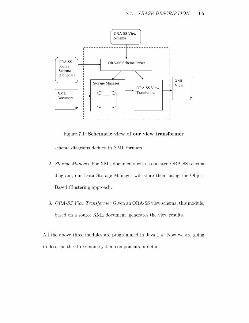
7.1. XBASE DESCRIPTION 65
Storage Manager
XML Document
ORA-SS Source Schema (Optional)
ORA-SS View Transformer
ORA-SS Schema Parser
ORA-SS View Schema
XML View
Figure 7.1: Schematic view of our view transformer
schema diagrams defined in XML formats.
2. Storage Manager For XML documents with associated ORA-SS schema
diagram, our Data Storage Manager will store them using the Object
Based Clustering approach.
3. ORA-SS View Transformer Given an ORA-SS view schema, this module,
based on a source XML document, generates the view results.
All the above three modules are programmed in Java 1.4. Now we are going
to describe the three main system components in detail.

7.1. XBASE DESCRIPTION 66
7.1.1 ORA-SS Schema Parser
In XBase, an ORA-SS schema diagram is defined in XML format. XML doc-
uments defining ORA-SS schema are then parsed and turned into data struc-
tures accessible by other system modules. As an example, the XML document
in Figure 7.2 is a valid XML document of the ORA-SS schema diagram in
Figure 2.2. The XML document is easy to understand because we can find
one-to-one mappings from the constructs used in the XML documents to the
ORA-SS schema diagram definition. At the outermost level, the XML docu-
ment consists of definitions of object classes. For each object class, we define
its names, the relationships it participates in, the attributes nested in the ob-
ject class and its child object classes. For each attribute, we use a field Key to
indicate if it is a key; a field called reln indicates the attribute is a relationship
attribute and its values tells the owner relationship of the attribute.
7.1.2 Storage Manager
Our XML document storage manager stores XML documents into a set of
sequential files. Each sequential file consists of objects of the same class. We
call each object in our system a record. The structure of each record is shown
in Figure 7.3. A record in our storage system have varied length. Each record
consists of a header and values of various fields which correspond to attributes
of the object contained in the record. A record header has the following parts:
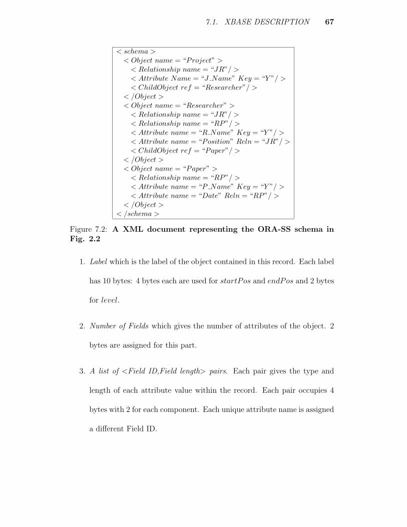
7.1. XBASE DESCRIPTION 67
< schema >< Object name = “Project” >
< Relationship name = “JR”/ >< Attribute Name = “J Name” Key = “Y ”/ >< ChildObject ref = “Researcher”/ >
< /Object >< Object name = “Researcher” >
< Relationship name = “JR”/ >< Relationship name = “RP”/ >< Attribute name = “R Name” Key = “Y ”/ >< Attribute name = “Position” Reln = “JR”/ >< ChildObject ref = “Paper”/ >
< /Object >< Object name = “Paper” >
< Relationship name = “RP”/ >< Attribute name = “P Name” Key = “Y ”/ >< Attribute name = “Date” Reln = “RP”/ >
< /Object >< /schema >
Figure 7.2: A XML document representing the ORA-SS schema inFig. 2.2
1. Label which is the label of the object contained in this record. Each label
has 10 bytes: 4 bytes each are used for startPos and endPos and 2 bytes
for level.
2. Number of Fields which gives the number of attributes of the object. 2
bytes are assigned for this part.
3. A list of <Field ID,Field length> pairs. Each pair gives the type and
length of each attribute value within the record. Each pair occupies 4
bytes with 2 for each component. Each unique attribute name is assigned
a different Field ID.
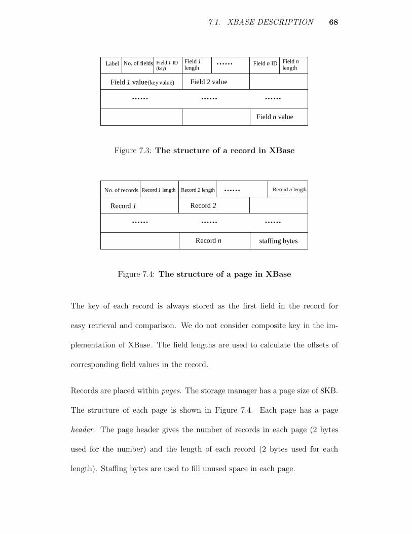
7.1. XBASE DESCRIPTION 68
Label No. of fields Field 1 ID (key)
Field 1 length
…… Field n ID Field n length
Field 1 value(key value) Field 2 value
Field n value
…… …… ……
Figure 7.3: The structure of a record in XBase
No. of records Record 1 length Record 2 length …… Record n length
Record 1 Record 2
Record n
…… …… ……
staffing bytes
Figure 7.4: The structure of a page in XBase
The key of each record is always stored as the first field in the record for
easy retrieval and comparison. We do not consider composite key in the im-
plementation of XBase. The field lengths are used to calculate the offsets of
corresponding field values in the record.
Records are placed within pages. The storage manager has a page size of 8KB.
The structure of each page is shown in Figure 7.4. Each page has a page
header. The page header gives the number of records in each page (2 bytes
used for the number) and the length of each record (2 bytes used for each
length). Staffing bytes are used to fill unused space in each page.

7.2. DATASETS 69
7.1.3 ORA-SS View Transformer
The ORA-SS view transformer of XBase implements various transformation
techniques we discussed in the previous chapter. It takes in an ORA-SS view
schema and accesses the data storage module and then performs view trans-
formation. The resulting views are output as XML documents.
7.2 Datasets
We use both real-world and synthetic XML data in our experiments.
7.2.1 DBLP Bibliography Record (DBLP)
DBLP[19] dataset is a real-world XML data source frequently used as bench-
mark dataset. It is a bibliography file (100 Mbytes in total size) which contains
about 380,000 computer science publications (journal articles, proceedings and
so on) and over 80,000 authors. The ORA-SS schema of the dataset is shown
in Figure 7.5.
7.2.2 Project-Researcher-Paper (JRP)
We synthesize the JRP dataset by our own XML data generator. In a JRP
data instance, on average one project has 5 researchers and each researcher has

7.2. DATASETS 70
PA;2
year journal
Publication
author
name
DBLP
pages url volume ee
title
Figure 7.5: The ORA-SS schema of DBLP Dataset
10 publications. For example, in a 20MByte JRP file, there are in total 2400
(distinct) project elements and 12,000 researcher elements (6,000 distinct) and
120,000 (60,000 distinct) paper elements. These numbers increase proportion-
ally with the size of JRP data file. The ORA-SS schema of the dataset is
shown in Figure 7.6.
Paper
Researcher
Project
R_Name
P_Name
J_Name
Position
JR;2
RP;2
Date
JR
Figure 7.6: The ORA-SS schema of JRP Dataset

7.3. PERFORMANCES AND ANALYSIS 71
7.3 Performances and Analysis
All our experiments were run on a 2.4GHz Pentium 4 processor with 512MB
memory. We primarily focus on two issues in our experiments. First we inves-
tigate the performance of Object Based Clustering in view processing. Next
we want to compare the performance of our view transformation system with
that of current popular XML query processing engines.
7.3.1 The advantages of OBC storage
Many native XML DBMSs use Element Based Clustering scheme. The scheme
stores all XML element with the same tag name or attribute values with the
same type in a cluster. On the other hand, the Object Based Clustering (OBC)
scheme groups attributes of an object together with the object itself. By
bundling attribute values with their owner objects, OBC allows more efficient
processing of XML queries.
Our experiment results confirm the above observation. We implement both
EBC and OBC storage schemes and use them to process queries on XML
documents. We test the queries in Table. 7.1 for an JRP dataset of 20M
bytes (135,000 elements) and the queries in Table. 7.2 for a DBLP dataset
of 100M bytes. The set of queries consists of both simple ones which are
mainly projections and complex ones. We choose queries with only Ancestor-
Descendant relationships because we are ultimately interested in processing

7.3. PERFORMANCES AND ANALYSIS 72
Q1 //Paper[P Name]
Q2 //Project[J Name]//Paper[P Name]
Q3 //Researcher[R Name]//Paper[P Name]
Q4 //Project[J Name]//Researcher[R Name]//Paper[P Name]
Table 7.1: XPath Queries on JRP dataset
Q1 //Author[text()]
Q2 //Publication[title]//Author[text()]
Q3 //Publication[title][year][journal][volume]//Paper[P Name]
Table 7.2: XPath Queries on DBLP dataset
ORA-SS view schemas which do not concern with Parent-Child relationships.
The running times of processing the above queries using OBC AND EBC
storage schemes can be seen from Figure 7.7 and Figure 7.8.
02468
101214161820
Exe
cuti
on T
ime(
Sec
)
Q1 Q2 Q3 Q4Query
OBCEBC
Figure 7.7: Comparison of XPath Query Processing on EBC and OBCStorage schemes using a JRP dataset of 20MB
From Figure 7.7 and 7.8, we can see that in most cases, OBC storage scheme

7.3. PERFORMANCES AND ANALYSIS 73
05
1015202530354045
Exe
cuti
on
Tim
e(S
ec)
Q1 Q2 Q3
Query
OBCEBC
Figure 7.8: Comparison of XPath Query Processing on EBC and OBCStorage schemes using a DBLP dataset of 100MB
can provide more efficient processing of XPath Query compared with EBC.
What is more, the more complex the query is, the more time saving that OBC
results. The only exception is the query Q2 in Figure 7.8: in this case under
the OBC scheme a publication object is bundled with many of its attributes
but only one of them title is required in the final results. Thus OBC causes
unnecessary I/O cost which is not a problem in EBC because EBC doesn’t
need to scan clusters whose elements or attribute values do not appear in
the query. Consequently, the additional I/O costs overtake the benefit of less
structural join. Interestingly, when we require more attributes of a publication
to be output as in Q3 of Figure 7.8, OBC now performs much better than
EBC because of less redundant I/O costs.

7.3. PERFORMANCES AND ANALYSIS 74
7.3.2 View Processing in XBase
We compare the view processing performance of XBase with state-of-art XML
query processing engines. Among many available candidates, we choose SAXON[26]
(version 7.5) XSLT processor and Quip[25] XQuery processor. SAXON is
the only XSLT engine available now which supports XSLT2.0[33] standard.
XSLT2.0 has features like grouping (i.e. < xsl : for − each − group > direc-
tive) which is important to view transformation operation like value join but
not present in the XSLT1.0. SAXON is implemented using Java and generally
considered as one of the fastest XSLT processors available. Quip is a complete
XQuery[32] processor freely available. XQuery has supports for grouping as
well (i.e. distinct− values() function in XQuery 1.0).
Project-Researcher-Paper(JRP)
We use the following four ORA-SS views (Figure 7.9) over the source schema
which range from simple projections to more complex swapping.
The performances of view transformation using XBase, SAXON and Quip are
shown from Figure 7.10 to Figure 7.16. Note that the running times of SAXON
and Quip include the time spent on loading source XML document.
DBLP
We use the following two ORA-SS views over the DBLP datasets:
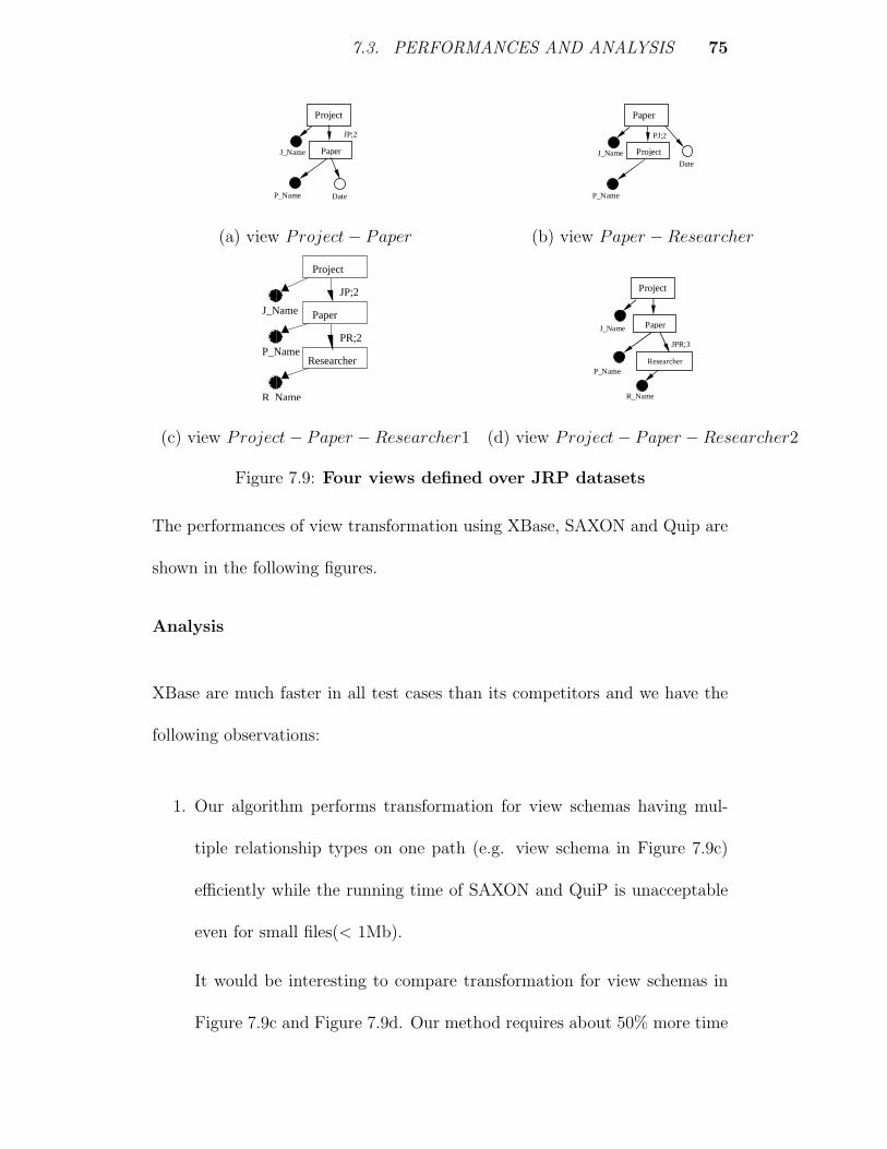
7.3. PERFORMANCES AND ANALYSIS 75
Paper
Project
P_Name
J_Name
JP;2
Date
Project
Paper
J_Name
PJ;2
Date
P_Name
(a) view Project− Paper (b) view Paper −Researcher
R_Name
P_Name
J_Name
PR;2
JP;2
Researcher
Paper
Project
����������������
����������������
����������������
����
����
����
Researcher
Paper
Project
R_Name
JPR;3
P_Name
J_Name
(c) view Project− Paper −Researcher1 (d) view Project− Paper −Researcher2
Figure 7.9: Four views defined over JRP datasets
The performances of view transformation using XBase, SAXON and Quip are
shown in the following figures.
Analysis
XBase are much faster in all test cases than its competitors and we have the
following observations:
1. Our algorithm performs transformation for view schemas having mul-
tiple relationship types on one path (e.g. view schema in Figure 7.9c)
efficiently while the running time of SAXON and QuiP is unacceptable
even for small files(< 1Mb).
It would be interesting to compare transformation for view schemas in
Figure 7.9c and Figure 7.9d. Our method requires about 50% more time

7.3. PERFORMANCES AND ANALYSIS 76
0
10
20
30
40
50
60
20 40 60 80
Source XML file size (MB)
Ru
nn
ing
Tim
e(se
c)
Xbase
SAXON
Quip
Figure 7.10: Running time comparison of processing ORASS viewschema in Fig. 7.9a for JRP dataset
0
10
20
30
40
50
60
70
20 40 60 80
Source XML file size (MB)
Ru
nn
ing
Tim
e(se
c)
Xbase
SAXON
Quip
Figure 7.11: Running time comparison of processing ORASS viewschema in Fig. 7.9b for JRP dataset
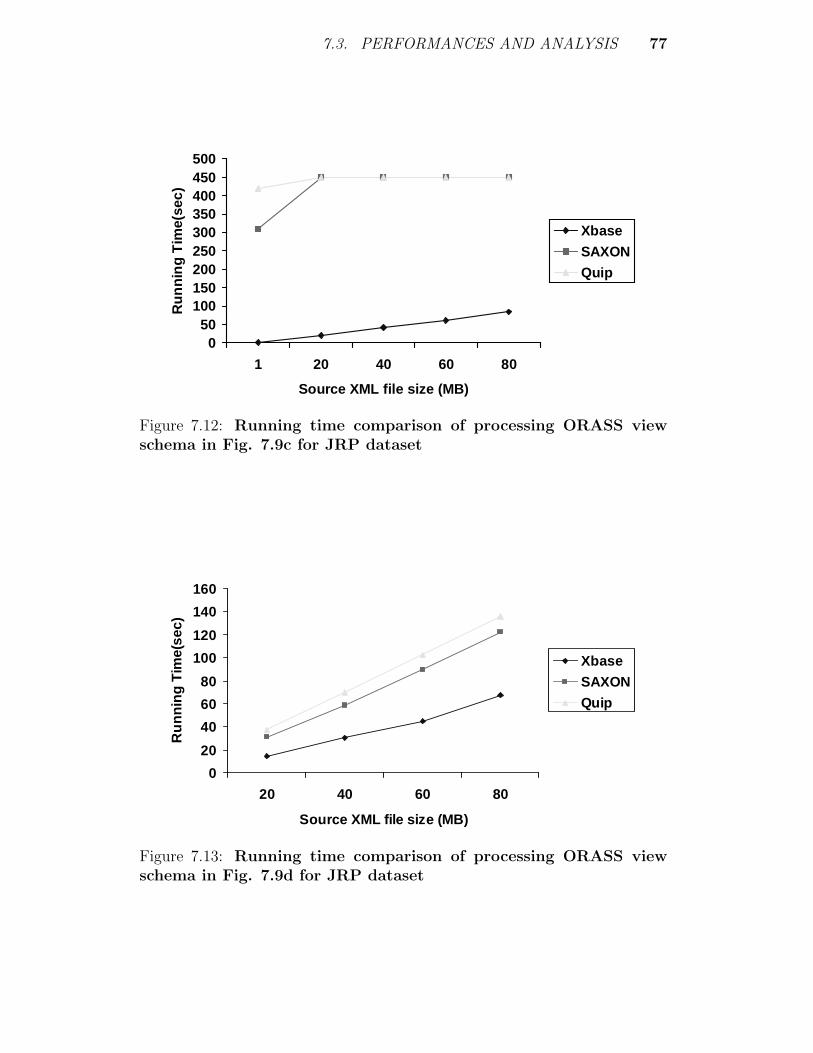
7.3. PERFORMANCES AND ANALYSIS 77
050
100150200250300350400450500
1 20 40 60 80
Source XML file size (MB)
Ru
nn
ing
Tim
e(se
c)
Xbase
SAXON
Quip
Figure 7.12: Running time comparison of processing ORASS viewschema in Fig. 7.9c for JRP dataset
0
20
40
60
80
100
120
140
160
20 40 60 80
Source XML file size (MB)
Ru
nn
ing
Tim
e(se
c)
Xbase
SAXON
Quip
Figure 7.13: Running time comparison of processing ORASS viewschema in Fig. 7.9d for JRP dataset

7.3. PERFORMANCES AND ANALYSIS 78
Author Author
Name Publication
year
Title
Name
AP;2
(a) View Author (b) View Author-Publication
Figure 7.14: Two views defined over DBLP datasets
0
20
40
60
80
100
120
140
160
20 40 60 80
Source XML file size (MB)
Ru
nn
ing
Tim
e(se
c)
Xbase
SAXON
Quip
Figure 7.15: Running time comparison of processing ORASS viewschema in Fig.7.14a for DBLP dataset
(Figure 7.10 and Figure 7.11)in view schema Figure7.9c because it has
one more relationship type than Figure 7.9d and consequently needs one
more round of associative join and value join. However, although SAXON
7.5 performs reasonably well in Figure7.9d, it simply takes too long to
finish views for Figure7.9c. This happens to Quip too. We list the XSLT
scripts used for both view schemas in Appendix I and II. The scripts
explain why XSLT engines like SAXON is slow for the view schema with
two binary relationship types but much quicker for the view schema with
one ternary relationship type. We extract the most important sections
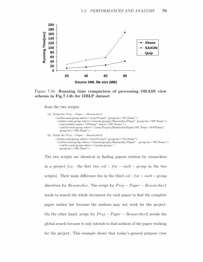
7.3. PERFORMANCES AND ANALYSIS 79
020406080
100120140160180200
20 40 60 80
Source XML file size (MB)
Ru
nn
ing
Tim
e(se
c)Xbase
SAXON
Quip
Figure 7.16: Running time comparison of processing ORASS viewschema in Fig.7.14b for DBLP dataset
from the two scripts:
(a) Script for Proj − Paper −Researcher1
<xsl:for-each-group select=“root/Project” group-by=“@J Name”><xsl:for-each-group select=“current-group()/Researcher/Paper” group-by=“@P Name”>
<xsl:variable name=“vPName” select=“@P Name”/><xsl:for-each-group select=“/root/Project/Researcher[Paper/@P Name =$vPName]”group-by=“@R Name”>
(b) Script for Proj − Paper −Researcher2
<xsl:for-each-group select=“root/Project” group-by=”@J Name”><xsl:for-each-group select=“current-group()/Researcher/Paper” group-by=“@P Name”>
<xsl:for-each-group select=“current-group/..”group-by=“@R Name”>
The two scripts are identical in finding papers written by researchers
in a project (i.e. the first two xsl : for − each − group in the two
scripts). Their main difference lies in the third xsl : for− each− group
directives for Researcher. The script for Proj − Paper − Researcher1
needs to search the whole document for each paper to find the complete
paper author list because the authors may not work for the project.
On the other hand, script for Proj − Paper − Researcher2 avoids the
global search because it only intends to find authors of the paper working
for the project. This example shows that today’s general purpose view

7.3. PERFORMANCES AND ANALYSIS 80
transformation engines still need more work on optimization.
2. Our algorithm is very efficient in views which project and swap over
portion but not all of the source data(e.g. views Project − Paper,
Paper − Project of JRP datasets and Author,Author − Publication
of DBLP datasets).
This is especially true with big files (e.g. 80MByte DBLP and JRP XML
files) approaching the memory threshold because to load the whole doc-
ument into the memory (which is what SAXON and QuiP do) degrades
the performance significantly.
3. Our algorithm shows little differences in performances for views differing
from each other only in their node structural order.
To illustrate this, let us look at the running times of views Project −
Paper and Paper − Project in Figure 7.10 and Figure 7.11. These two
view schemas only differ on their node order. Our algorithm uses roughly
the same amount of time (about -2 5% of difference) on both views for
all file sizes; on the other hand, SAXON need about 20% more time
to process view Paper − Project. The reason for the big difference in
running times of SAXON and QuiP engines is due to their “tree-walk”
transformation mechanism: different orders in views cause different tree
traversal sequences. However, the running time of associative and value
join and merge operation in the transformation algorithms of XBase are

7.3. PERFORMANCES AND ANALYSIS 81
determined solely by the total list sizes.

Chapter 8
Conclusion
The starting point of our work is the observation of problems with two kinds
of XML view transformation systems. High level systems like eXcelon[11] and
Clio[24], which perform view transformations by defining target view schema,
have problems with not being able to define views with complex semantics. On
the other hand, general systems like XSLT and XQuery processors require the
user to write transformation scripts themselves. The problem becomes worse
with tree-structured XML data because many possible structural variants need
to be considered in transformation scripts to cover all possible query results.
As we have demonstrated in experiments, it is hard for the systems to optimize
many simple and practical XSLT/XQuery scripts.
Our approach, like the other high-level systems, allows users to define view
schema to get desired views. However, our method differs from other high-
level XML view transformation system in the following aspects:
1. The use of ORA-SS as underlying schema representation allows us to
82

Chapter 8. Conclusion 83
express view schemas with a great variety of semantic meanings.
2. Our ontology-based view definition approach saves users the trouble of
looking into often complicated source schema. Users just need to know
the set of element names (ontology) in the source schema to define views.
Mapping from source schema to view schema is done by our system.
3. It performs view transformation directly on a native XML DBMS: XBase.
Other systems usually convert schema mapping into XSLT/XQuery scripts
and still rely on XSLT/XQuery engines to perform transformation.
At the same time, based on ORA-SS schemas, our system requires much less
time than general XML processors in processing view transformations.
Our view transformation engine XBase has many novel features. Our stor-
age method Object Based Clustering allows us to leverage on the new join
processing techniques naturally. In most view transformations, only the rele-
vant portions of source document are read. ORA-SS, as the conceptual model
used in our transformation, differs from other traditional structure-based XML
data models by taking into full consideration the semantic information such
as keys, relationship and relationship attribute associated with XML data. In
our transformation method, a relationship type in ORA-SS schema is the ba-
sic unit of transformation. We devise novel and efficient join technique called
associative join to construct a single relationship type.
From a performance point of view, our transformation engine XBase is much

Chapter 8. Conclusion 84
more efficient compared with XQuery/XSLT engines. In particular, our method
is very fast in projection and swapping over portion of source data because it
only loads data which is required. In comparison, today’s XSLT and XQuery
processors are slow in processing view operations like projection and swap-
ping. Our method is also much faster in processing ORA-SS view schema with
multiple relationships on a single path.
Our work can be extended in several directions. View operations like value se-
lection, negation and so on are not considered in our prototype. Meanwhile in
our view transformation algorithms, we do not utilize source ORA-SS schema
information, which can help to further optimize our view transformation en-
gine.

Bibliography
[1] N. Bruno, N. Koudas, and D. Srivastava. Holistic twig joins: optimal
XML pattern matching. In Proceedings of SIGMOD 2002, pages 310–321,
2002.
[2] S. Ceri, S. Comai, E. Damiani, P. Fraternali, S. Paraboschi, and L.Tanca.
XML-GL: a graphical language of querying and restructuring XML doc-
uments. In Proceedings of WWW8, pages 1171–1187, 1999.
[3] J. Chen, D. J. DeWitt, F. Tian, and Y. Wang. NiagaraCQ: A scalable con-
tinuous query system for internet databases. In Proceedings of SIGMOD
2000, pages 379–390, 2000.
[4] Q. Chen, A. Lim, and K. W. Ong. D(k)-index: An adaptive structural
summary for graph-structured data. In Proceedings of SIGMOD 2003,
pages 134–144, 2003.
[5] T. Chen, T. W. Ling, and C. Y. Chan. Prefix path streaming: a new
clustering method for optimal XML twig pattern matching. In Proceedings
of DEXA 2004, pages 801–811, 2004.
85

BIBLIOGRAPHY 86
[6] Y. B. Chen, T. W. Ling, and M. L. Lee. Designing valid XML views. In
Proceeding of ER 2002, pages 463–478, 2002.
[7] Y. B. Chen, T. W. Ling, and M. L. Lee. Automatic generation of XQuery
view definitions from ORA-SS views. In Proceeding of ER 2003, pages
158–171, 2003.
[8] J. Clark. XT XSLT processor. http://blnz.com/xt/.
[9] G. Dobbie, X. Wu, T. W. Ling, and M. L. Lee. ORA-SS: An Object-
Relationship-Attribute model for Semistructured data. Technical Report
TR21/00, School of Computing, National University of Singapore, 2000.
[10] DTD. Document type definitions. http://www.w3.org/TR/REC-xml.
[11] eXcelon. An general XML data manager. http://www.exceloncorp.com/.
[12] R. Goldman and J. Widom. Dataguides: Enabling query formulation and
optimization in semistructured databases. In Proceedings of VLDB 97,
pages 436–445, 1997.
[13] H. He and J. Yang. Multiresolution indexing of XML for frequent queries.
In Proceedings of ICDE 2004, pages 683–694, 2004.
[14] H. V. Jagadish and S. AL-Khalifa. TIMBER: A native XML database.
Technical report, University of Michigan, 2002.
[15] H. Jiang, W. Wang, H. Lu, and J. X. Yu. Holistic twig joins on indexed
XML documents. In In Proceeding of VLDB 2003, pages 273–284, 2003.

BIBLIOGRAPHY 87
[16] C. C. Kanne and G. Moerkotte. Efficient storage of XML data. In Pro-
ceedings of ICDE 2000, pages 198–209, 2000.
[17] R. Kaushik, P. Sheony, P. Bohannon, and E. Gudes. Exploiting local
similarity for efficient indexing of paths in graph structured data. In
Proceedings of ICDE 2002, pages 129–140, 2002.
[18] M. Ley. Apache Xindice. http://XML.apache.org/xindice/.
[19] M. Ley. DBLP computer science bibliography record.
http://www.informatik.uni-trier.de/ ley/db/.
[20] D. F. Luo, T. Chen, T. W. Ling, and X. F. Meng. On view transformation
support for a native XML DBMS. In Proceeding of DASFAA 2004, pages
226–231, 2004.
[21] J. McHugh, S. Abiteboul, R. Goldman, D. Quass, and J. Widom. Lore: A
database management system for semistructured data. SIGMOD Record,
pages 54–66, 1997.
[22] T. Milo and D. Suciu. Index structures for path expressions. In Proceed-
ings of ICDT 99, pages 277–295, 1999.
[23] W. Ni and T. W. Ling. GLASS: A graphical query language for semi-
structured data. In Proceedings o DASFAA 2003, pages 363–372, 2003.
BIBLIOGRAPHY 88
[24] L. Popa, M. A. Hernandez, Y. Velegrakis, R. J. Miller, F. Naumann, and
H. Ho. Mapping XML and relational schemas with Clio. In Proceedings
of ICDE 2002, pages 498–499, 2002.
[25] QuiP. http://developer.softwareag.com/tamino/quip/.
[26] SAXON. a XSLT processor. http://saxon.sourceforge.net/.
[27] X. Schema. XML Schema. http://www.w3.org/XML/Schema.
[28] H. Schoning. Tamino - a DBMS designed for XML. In Proceedings of
ICDE 2001, pages 149–154, 2001.
[29] Y. Wu, J. M. Patel, and H. V. Jagadish. Structural join order selection for
XML query optimization. In Proceedings of ICDE 2003, pages 443–454,
2003.
[30] Xalan. XSLT processor. http://xml.apache.org/xalan-j/.
[31] XPath. http://www.w3.org/TR/xpath.
[32] XQuery. http://www.w3.org/XML/Query.
[33] XSLT. http://www.w3.org/Style/XSL/.
[34] C. Zhang, J. F. Naughton, D. J. DeWitt, Q. Luo, and G. M. Lohman.
On supporting containment queries in relational database management
systems. In Proceedings of SIGMOD 2001, pages 425–436, 2001.

Appendix A
Appendix
A.1 XSLT Script for view schema in Figure
7.9c:
Remark: The differences of XSLT scripts in Appendix I and II are highlighted
lines.
<xsl:transform><xsl:template match=“/”><root>
<xsl:for-each-group select=“root/Project” group-by=“@J Name”¿<Project>
<J Name><xsl:value-of select=“@J Name”/></J Name><xsl:for-each-group select=“current-group()/Researcher/Paper” group-by=“@P Name”><Paper>
<xsl:variable name=“vPName” select=“@P Name”/><P Name><xsl:value-of select=“@P Name”/></P Name>
<xsl:for-each-group select=“/root/Project/Researcher[Paper/@P Name =$vPName]”group-by=“@R Name”>
<Researcher><R Name><xsl:value-of select=”@R Name”/></R Name>
</Researcher></xsl:for-each-group>
</Paper></xsl:for-each-group>
</Project></xsl:for-each-group>
</root></xsl:template>
</xsl:transform>
89

A.2. XSLT SCRIPT FOR VIEW SCHEMA IN FIGURE 7.9D: 90
A.2 XSLT Script for view schema in Figure
7.9d:
Remark: The differences of XSLT scripts in Appendix I and II are highlighted
lines.
<xsl:transform><xsl:template match=“/”><root>
<xsl:for-each-group select=“root/Project” group-by=“@J Name”¿<Project>
<J Name><xsl:value-of select=“@J Name”/></J Name><xsl:for-each-group select=“current-group()/Researcher/Paper” group-by=“@P Name”><Paper>
<xsl:variable name=“vPName” select=“@P Name”/><P Name><xsl:value-of select=“@P Name”/></P Name>
<xsl:for-each-group select=“current-group()/..” group-by=“@R Name”><Researcher>
<R Name><xsl:value-of select=”@R Name”/></R Name></Researcher></xsl:for-each-group>
</Paper></xsl:for-each-group>
</Project></xsl:for-each-group>
</root></xsl:template>
</xsl:transform>