on vectorization of deep convolutional neural networks for vision...
TRANSCRIPT

On Vectorization of Deep Convolutional Neural Networks for Vision Tasks
Jimmy SJ. Ren Li XuLenovo Research & Technology
http://[email protected] [email protected]
AbstractWe recently have witnessed many ground-breaking re-sults in machine learning and computer vision, gen-erated by using deep convolutional neural networks(CNN). While the success mainly stems from the largevolume of training data and the deep network architec-tures, the vector processing hardware (e.g. GPU) undis-putedly plays a vital role in modern CNN implemen-tations to support massive computation. Though muchattention was paid in the extent literature to understandthe algorithmic side of deep CNN, little research wasdedicated to the vectorization for scaling up CNNs. Inthis paper, we studied the vectorization process of keybuilding blocks in deep CNNs, in order to better under-stand and facilitate parallel implementation. Key stepsin training and testing deep CNNs are abstracted as ma-trix and vector operators, upon which parallelism can beeasily achieved. We developed and compared six imple-mentations with various degrees of vectorization withwhich we illustrated the impact of vectorization on thespeed of model training and testing. Besides, a unifiedCNN framework for both high-level and low-level vi-sion tasks is provided, along with a vectorized Mat-lab implementation with state-of-the-art speed perfor-mance.
IntroductionDeep convolutional neural network (CNN) has become akeen tool in addressing large scale artificial intelligencetasks. Though the study of CNN can be traced back to late1980s (LeCun et al. 1989; 1990), the recent success of deepCNN is largely attributed to the concurrent progresses of thetwo technical streams. On the one hand, the new deep CNNarchitecture with elements such as Dropout (Hinton et al.2012; Krizhevsky, Sutskever, and Hinton 2012), DropCon-nect (Wan et al. 2013), Rectified Linear Units-ReLU (Nairand Hinton 2010) as well as new optimization strategies(Dean et al. 2012) have empowered deep CNN with greaterlearning capacity. On the other hand, the rapid advances anddemocratization of high performance general purpose vectorprocessing hardware, typified by graphics processing unit(GPU), unleashes the potential power of deep CNN by scal-ing up the network significantly.
Copyright c© 2015, Association for the Advancement of ArtificialIntelligence (www.aaai.org). All rights reserved.
Various infrastructures were used in scaling up deepCNNs, including GPU (Coates et al. 2013), distributed CPUbased framework (Dean et al. 2012), FPGA (Farabet et al.2009), etc. Though the implementation details among thoseapproaches differ, the core insight underlying the idea ofscaling up deep CNN is parallelization (Bengio and Le-Cun 2007) in which vectorization technique is the funda-mental element. While the consecutive distinguished perfor-mance of GPU trained CNNs in the ImageNet visual recog-nition challenge (Krizhevsky, Sutskever, and Hinton 2012;Russakovsky et al. 2013) as well as the reported results inmany studies in the literature justify its effectiveness (Jiaet al. 2014; Sermanet et al. 2013), the published literaturedid not provide sufficient insights on how the vectorizationwas carried out in detail. We also found there is no previ-ous study to answer how different degrees of vectorizationinfluence the performance of deep CNN, which is, however,crucial in finding the bottlenecks and helps to scale up thenetwork architecture. We believe these questions form a sig-nificant research gap and the answer to these questions shallshed some light on the design, tuning and implementation ofvectorized CNNs.
In this paper, we reinterpret the key operators in deepCNNs in vectorized forms with which high parallelism canbe easily achieved given basic parallelized matrix-vector op-erators. To show the impact of the vectorization on the speedof both model training and testing, we developed and com-pared six implementations of CNNs with various degreesof vectorization. We also provide a unified framework forboth high-level and low-level vision applications includingrecognition, detection, denoise and image deconvolution.Our Matlab Vectorized CNN implementation (VCNN) willbe made publicly available on the project webpage.
Related WorkEfforts on speeding up CNN by vectorization starts with itsinception. Specialized CNN chip (Jackel et al. 1990) wasbuilt and successfully applied to handwriting recognition inthe early 90s. Simard et al. (2003) simplified CNN by fusingconvolution and pooling operations. This speeded up the net-work and performed well in document analysis. Chellapillaet al. (2006) adopted the same architecture but unrolled theconvolution operation into a matrix-matrix product. It hasnow been proven that this vectorization approach works par-

ticularly well with modern GPUs. However, limited by theavailable computing power, the scale of the CNN exploredat that time was much smaller than modern deep CNNs.
When deep architecture showed its ability to effectivelylearn highly complex functions (Hinton, Osindero, and Teh2006), scaling up neural network based models was soonbecoming one of the major tasks in deep learning (Bengioand LeCun 2007). Vectorization played an important role inachieving this goal. Scaling up CNN by vectorized GPU im-plementations such as Caffe (Jia et al. 2014), Overfeat (Ser-manet et al. 2013), CudaConvnet (Krizhevsky, Sutskever,and Hinton 2012) and Theano (Bergstra et al. 2010) gener-ates state-of-the-art results on many vision tasks. Albeit thegood performance, few of the previous papers elaborated ontheir vectorization strategies. As a consequence, how vec-torization affects design choices in both model training andtesting is unclear.
Efforts were also put in the acceleration of a part of thedeep CNN from algorithmic aspects, exemplified by the sep-arable kernels for convolution (Denton et al. 2014) and theFFT speedup (Mathieu, Henaff, and LeCun 2013). Insteadof finding a faster alternative for one specific layer, we fo-cus more on the general vectorization techniques used in allbuilding blocks in deep CNNs, which is instrumental notonly in accelerating existing networks, but also in providingguidance for implementing and designing new CNNs acrossdifferent platforms, for various vision tasks.
Vectorization of Deep CNNVectorization refers to the process that transforms the orig-inal data structure into a vector representation so that thescalar operators can be converted into a vector implementa-tion. In this section, we introduce vectorization strategies fordifferent layers in Deep CNNs.
Figure 1 shows the architecture of a typical deep CNN forvision tasks. It contains all of the essential parts of modernCNNs. Comprehensive introductions on CNN’s general ar-chitecture and the recent advances can be found in (LeCunet al. 1998) and (Krizhevsky, Sutskever, and Hinton 2012).
We mark the places where vectorization plays an impor-tant role. “a” is the convolution layer that transforms the in-put image into feature representations, whereas “b” is theone to handle the pooling related operations. “c” representsthe convolution related operations for feature maps. We willsee shortly that the vectorization strategies between “a” and“c” are slightly different. “d” involves operations in the fullyconnected network. Finally, “e” is the vectorization opera-tion required to simultaneously process multiple input sam-ples (e.g. mini-batch training). It is worth noting that weneed to consider both forward pass and back-propagationfor all these operations.
Vectorizing ConvolutionWe refer to the image and intermediate feature maps as f ,one of the convolution kernels as wi, the convolution layercan be typically expressed as
f l+1i = σ(wl
i ∗ f l + bli), (1)
ab c
d
e
convolution pooling convolution pooling fully connected
Figure 1: Convolutional Neural Network architecture for vi-sual recognition.
where i indexes the ith kernel. l indexes the layer. bl is thebias weight. ∗ is the convolution operator. For vision tasks,f can be 2- or 3-dimension. The outputs from previous layercan be deemed as one single input f l. σ is the nonlinearfunction which could be ReLU, hyperbolic tangent, sigmoid,etc. Adding bias weight and applying nonlinear mappingare element-wise operations which can be deemed as al-ready fully vectorized, i.e. the whole feature vector can beprocessed simultaneously. Contrarily, the convolution oper-ators involve a bunch of multiplication with conflict mem-ory access. Even the operators are parallized for each pixel,the parallelism (Ragan-Kelley et al. 2013) to be exploited israther limited: compared to the number of computing unitson GPU, the number of convolution in one layer is usuallysmaller. A fine-grained parallelism on element-wise multi-plication is much preferred, leading to the vectorization pro-cess to unroll the convolution.
In what follows, all the original data f , b and w can beviewed as data vectors. Specifically, we seek vectorizationoperators ϕc() to map kernel or feature map to its matrixform so that convolution can be conducted by matrix-vectormultiplication. However, a straight forward kernel-matrix,image-vector product representation of convolution is notapplicable here, since the kernel matrix is a sparse block-Toeplitz-Toeplitz-block one, not suitable for parallelizationdue to the existence of many zero elements. Thanks to theduality of kernel and feature map in convolution, we canconstruct a dense feature-map-matrix and a kernel-vector.Further, multiple kernels can be put together to form a ma-trix so as to generate multiple feature map outputs simulta-neously,
[f l+1i ]i = σ(ϕc(f
l)[wli]i + [bli]i). (2)
Operator [ ]i is to assemble vectors with index i to form amatrix.
Backpropagation The training procedure requires thebackward propagation of gradients through ϕc(f
l). Notethat ϕc(f
l) is in the unrolled matrix form, different form theoutputs of previous layer [f li ]i. An inverse operator ϕ−1
c ()is thus required to transform the matrix-form gradients intothe vector form for further propagation. Since ϕc() is a one-to-many mapping, ϕ−1
c () is a many-to-one operator. Fortu-nately, the gradient update is a linear process which can alsobe processed separately and combined afterwards.
Matlab Practice Our matlab implementation to vectorizethe input image is shown in Fig. 2. Specifically, we first cropthe image patches base on the kernel size and reorganize
1
2
3
4
5
6
7
8
9
1
2 3
4
5
6
7
8 9
4
5
2
5
5
6
8
k11 k 13k 12 k 14
k21 k 23k 22 k 24
k 31 k 33k 32 k 34
kernel1
kernel2
kernel3
f11 f13f12 f14
f21 f23f22 f24
f31 f33f32 f34
=
map1
map2
map3
Input
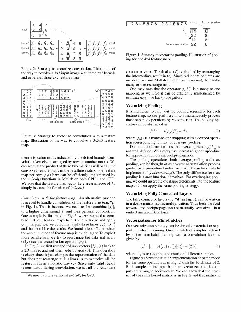
Figure 2: Strategy to vectorize convolution. Illustration ofthe way to covolve a 3x3 input image with three 2x2 kernelsand generates three 2x2 feature maps.
1
2
3
4
5
6
7
8
9
2
3
4
5
6
7
8
91 2
3
4
5
6
7
8
91
1
2
3
4
5
6
7
8
9
2
3
4
5
6
7
8
9
1
3
4
5
6
7
8
9
1
2
1
2 3
4
5 6
7
8 9
2
5
4
5
5
6
8
2
3 4
5
6 7
8
9 1
3
6
5
6
6
7
9
3
4 5
6
7 8
9
1 2
4
7
6
7
7
8
12
3 4
7
8
8
9
3 3
4 5
8
9
9
1
4
1
2 3
4
5 6
7
8 9
2
5
4
5
5
6
8
2
3 4
5
6 7
8
9 1
3
6
5
6
6
7
9
3
4 5
6
7 8
9
1 2
4
7
6
7
7
8
1set to zeros set to zeros
(a)
(b)
( c)
(d)
Figure 3: Strategy to vectorize convolution with a featuremap. Illustration of the way to convolve a 3x3x3 featuremap.
them into columns, as indicated by the dotted bounds. Con-volution kernels are arranged by rows in another matrix. Wecan see that the product of these two matrices will put all theconvolved feature maps in the resulting matrix, one featuremap per row. ϕc() here can be efficiently implemented bythe im2col() functions in Matlab on both GPU 1 and CPU.We note that the feature map vector here are transpose of fi,simply because the function of im2col().
Convolution with the feature map An alternative practiceis needed to handle convolution of the feature map (e.g. “c”in Fig. 1). This is because we need to first combine [f li ]ito a higher dimensional f l and then perform convolution.One example is illustrated in Fig. 3, where we need to com-bine 3 3 × 3 feature maps to a 3 × 3 × 3 one and applyϕc(). In practice, we could first apply three times ϕc() to f liand then combine the results. We found it less efficient sincethe actual number of feature map is much larger. To exploitmore parallelism, we try to reorganize the data and applyonly once the vectorization operator ϕc().
In Fig. 3, we first reshape column vectors [fi]i (a) back toa 2D matrix and put them side by side (b). This operationis cheap since it just changes the representation of the databut does not rearrange it. It allows us to vectorize all thefeature maps in a holistic way (c). Since only valid regionis considered during convolution, we set all the redundant
1We used a custom version of im2col() for GPU.
1 5 62 3 74 8
14
1422
22
68
for average pooling
for max pooling1 5 62 3 74 8
68
Figure 4: Strategy to vectorize pooling. Illustration of pool-ing for one 4x4 feature map.
columns to zeros. The final ϕc(f) is obtained by rearrangingthe intermediate result in (c). Since redundant columns areinvolved, we use Matlab function accumarray() to handlemany-to-one rearrangement.
One may note that the operator ϕ−1c () is a many-to-one
mapping as well. So it can be efficiently implemented byaccumarray(), for backpropagation.
Vectorizing PoolingIt is inefficient to carry out the pooling separately for eachfeature map, so the goal here is to simultaneously processthose separate operations by vectorization. The pooling op-erator can be abstracted as
f l+1 = σ(ϕp(fl) + bl), (3)
where ϕp() is a many-to-one mapping with a defined opera-tion corresponding to max- or average- pooling.
Due to the information loss, the inverse operator ϕ−1p () is
not well defined. We simply use nearest neighbor upscalingfor approximation during backpropagation.
The pooling operations, both average pooling and maxpooling, can be thought of as a vector accumulation processguided by a pre-defined index map, which can be similarlyimplemented by accumarray(). The only difference for maxpooling is a max function is involved. For overlapping pool-ing, we could insert the overlapped elements into the featuremap and then apply the same pooling strategy.
Vectorizing Fully Connected LayersThe fully connected layers (i.e. “d” in Fig. 1), can be writtenin a dense matrix-matrix multiplication. Thus both the feedforward and backpropagation are naturally vectorized, in aunified matrix-matrix form.
Vectorization for Mini-batchesOur vectorization strategy can be directly extended to sup-port mini-batch training. Given a batch of samples indexedby j, the mini-batch training with a convolution layer isgiven by
[f l+1i ]i = σ([ϕc(f
l,j)]j [w
li]i + [bli]i), (4)
where [ ]j is to assemble the matrix of different samples.Figure 5 shows the Matlab implementation of batch mode
for the same operation as in Fig. 2 with the batch size of 2.Both samples in the input batch are vectorized and the out-puts are arranged horizontally. We can show that the prod-uct of the same kernel matrix as in Fig. 2 and this matrix is
1
2 3
4
5
6
7
8 9
4
5
2
5
5
6
8
k 11 k13k 12 k14
k 21 k 23k 22 k 24
k 31 k 33k 32 k 34
kernel1
kernel2
kernel3
f11 f13f12 f14
f21 f23f22 f24
f31 f33f32 f34
=
map1
map2
map3
Input
1
2 3
4
5
6
7
8 9
4
5
2
5
5
6
8
7
8
9
1
2
3
4
5
6
7
8
9
f’11 f’13f’12 f’14
f’21 f’23f’22 f’24
f’31 f’33f’32 f’34
sample 1 sample 2
feature mapsfor sample 1
feature mapsfor sample 2
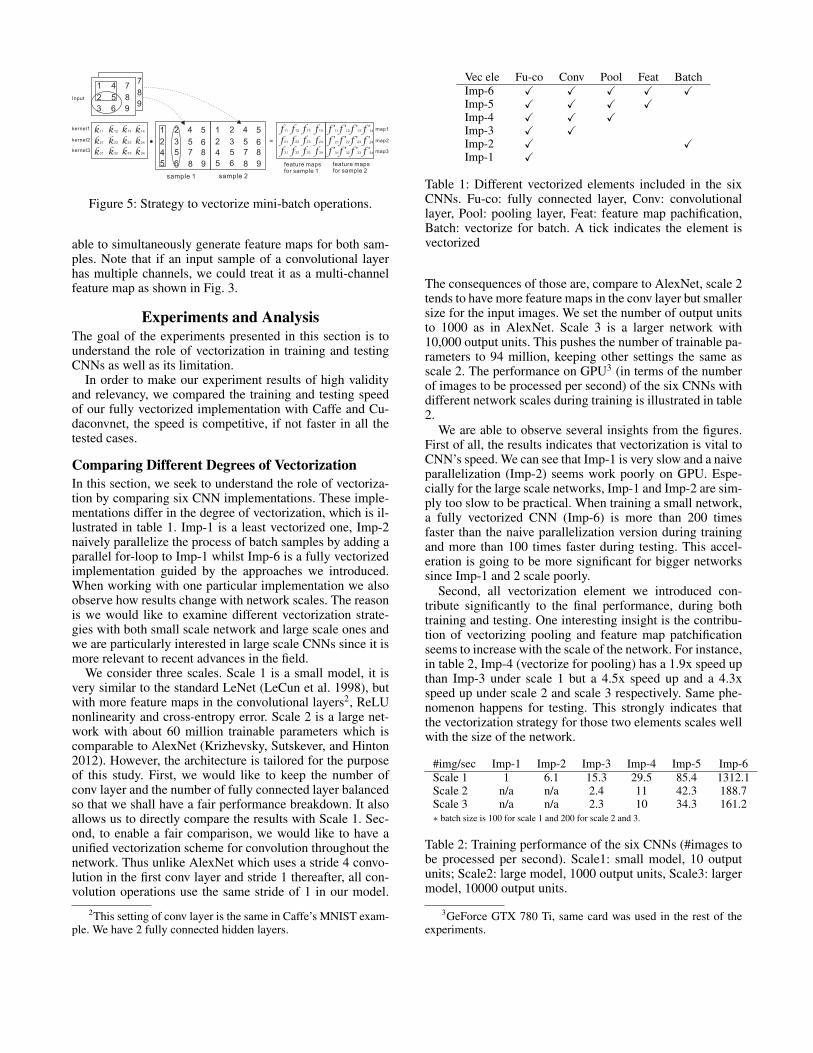
Figure 5: Strategy to vectorize mini-batch operations.
able to simultaneously generate feature maps for both sam-ples. Note that if an input sample of a convolutional layerhas multiple channels, we could treat it as a multi-channelfeature map as shown in Fig. 3.
Experiments and AnalysisThe goal of the experiments presented in this section is tounderstand the role of vectorization in training and testingCNNs as well as its limitation.
In order to make our experiment results of high validityand relevancy, we compared the training and testing speedof our fully vectorized implementation with Caffe and Cu-daconvnet, the speed is competitive, if not faster in all thetested cases.
Comparing Different Degrees of VectorizationIn this section, we seek to understand the role of vectoriza-tion by comparing six CNN implementations. These imple-mentations differ in the degree of vectorization, which is il-lustrated in table 1. Imp-1 is a least vectorized one, Imp-2naively parallelize the process of batch samples by adding aparallel for-loop to Imp-1 whilst Imp-6 is a fully vectorizedimplementation guided by the approaches we introduced.When working with one particular implementation we alsoobserve how results change with network scales. The reasonis we would like to examine different vectorization strate-gies with both small scale network and large scale ones andwe are particularly interested in large scale CNNs since it ismore relevant to recent advances in the field.
We consider three scales. Scale 1 is a small model, it isvery similar to the standard LeNet (LeCun et al. 1998), butwith more feature maps in the convolutional layers2, ReLUnonlinearity and cross-entropy error. Scale 2 is a large net-work with about 60 million trainable parameters which iscomparable to AlexNet (Krizhevsky, Sutskever, and Hinton2012). However, the architecture is tailored for the purposeof this study. First, we would like to keep the number ofconv layer and the number of fully connected layer balancedso that we shall have a fair performance breakdown. It alsoallows us to directly compare the results with Scale 1. Sec-ond, to enable a fair comparison, we would like to have aunified vectorization scheme for convolution throughout thenetwork. Thus unlike AlexNet which uses a stride 4 convo-lution in the first conv layer and stride 1 thereafter, all con-volution operations use the same stride of 1 in our model.
2This setting of conv layer is the same in Caffe’s MNIST exam-ple. We have 2 fully connected hidden layers.
Vec ele Fu-co Conv Pool Feat BatchImp-6 X X X X XImp-5 X X X XImp-4 X X XImp-3 X XImp-2 X XImp-1 X
Table 1: Different vectorized elements included in the sixCNNs. Fu-co: fully connected layer, Conv: convolutionallayer, Pool: pooling layer, Feat: feature map pachification,Batch: vectorize for batch. A tick indicates the element isvectorized
The consequences of those are, compare to AlexNet, scale 2tends to have more feature maps in the conv layer but smallersize for the input images. We set the number of output unitsto 1000 as in AlexNet. Scale 3 is a larger network with10,000 output units. This pushes the number of trainable pa-rameters to 94 million, keeping other settings the same asscale 2. The performance on GPU3 (in terms of the numberof images to be processed per second) of the six CNNs withdifferent network scales during training is illustrated in table2.
We are able to observe several insights from the figures.First of all, the results indicates that vectorization is vital toCNN’s speed. We can see that Imp-1 is very slow and a naiveparallelization (Imp-2) seems work poorly on GPU. Espe-cially for the large scale networks, Imp-1 and Imp-2 are sim-ply too slow to be practical. When training a small network,a fully vectorized CNN (Imp-6) is more than 200 timesfaster than the naive parallelization version during trainingand more than 100 times faster during testing. This accel-eration is going to be more significant for bigger networkssince Imp-1 and 2 scale poorly.
Second, all vectorization element we introduced con-tribute significantly to the final performance, during bothtraining and testing. One interesting insight is the contribu-tion of vectorizing pooling and feature map patchificationseems to increase with the scale of the network. For instance,in table 2, Imp-4 (vectorize for pooling) has a 1.9x speed upthan Imp-3 under scale 1 but a 4.5x speed up and a 4.3xspeed up under scale 2 and scale 3 respectively. Same phe-nomenon happens for testing. This strongly indicates thatthe vectorization strategy for those two elements scales wellwith the size of the network.
#img/sec Imp-1 Imp-2 Imp-3 Imp-4 Imp-5 Imp-6Scale 1 1 6.1 15.3 29.5 85.4 1312.1Scale 2 n/a n/a 2.4 11 42.3 188.7Scale 3 n/a n/a 2.3 10 34.3 161.2∗ batch size is 100 for scale 1 and 200 for scale 2 and 3.
Table 2: Training performance of the six CNNs (#images tobe processed per second). Scale1: small model, 10 outputunits; Scale2: large model, 1000 output units, Scale3: largermodel, 10000 output units.
3GeForce GTX 780 Ti, same card was used in the rest of theexperiments.

On the other hand, we also observe that vectorizing batchprocessing brings more than 10x speed up for small modelsbut only 3x to 5x speed up for large scale models. The con-tribution of vectorizing batch processing to the performanceseems to decrease when scaling up the network though thespeed up remains significant. We further investigate this phe-nomenon in the next section which leads to a strategy toachieve optimal training and testing speed.
In Search of Optimal SpeedWe investigated the puzzle of decelerating speed up by scru-tinizing the performance against different batch sizes. Theresults are presented in table 3 and 4 for training and testingrespectively.
#img/sec b=1 b=100 b=200 b=300 b=400Scale 1 88.5 1312 1450.9 1574.2 1632.8Scale 2 41.9 136.9 188.7 192.3 106.3Scale 3 34.3 123.5 161.3 163.9 91
Table 3: Training performance of Imp-6 against differentbatch sizes (#images to be processed per second).
#img/sec b=1 b=100 b=200 b=400 b=600Scale 1 151.5 1812.6 1878.4 2023.5 2192.2Scale 2 75.8 222.2 270.2 285.7 103.1Scale 3 74 212.8 256.4 277.8 89.2
Table 4: Test performance of Imp-6 against different batchsizes (#images to be processed per second).
In table 3, we can see that for the small model (scale 1) theacceleration brought by each adjacent batch size increase is14x, 1.1x, 1.08x and 1.03x. The acceleration obtained viathe increase of batch size seems to be rapidly vanishing.For the large model (scale 2), the first three acceleration ra-tio are 3.2x, 1.3x and 1.02x, demonstrating the same van-ishing trend. Further increase in batch size even leads to aperformance degradation instead. Same situation occurs forthe larger model (scale 3). Though the ability of processing192 images/second for training and 285 images/second fortesting with our commodity GPU for the scale 2 network ispromising, this result still indicates that there is some scal-ing limitation within the vectorization for batch processing.Similar results in table 4 seems to further suggest that suchlimitation is shared between training and testing. In order tocompletely understand the rationale under the hood, we haveto resort to a detailed performance breakdown.
Performance Breakdown and Limitation. We decom-pose the whole training procedure into the following com-ponents. They are 1) conv layers; 2) pooling layers; 3) fullyconnected layers; 4) others (e.g. ReLU, cost). We distinguishthe statistics between forward pass and back-propagation,therefore 8 components to look at.
Figure 6 illustrates the performance break down (in termsof the proportion of computing time in processing one batch)during training of the two representative cases from ourlargest network (scale 3) in the experiment. Batch size is
(a) (b) (c)
Figure 6: Performance break down. (a) Scale 3 network,batch size = 1. (b) Scale 3 network, batch size = 200. (c)Scale 3 network, batch size = 300. conv: conv layers, pool:pooling layers, full: fully connected layers, other: other op-erations, f : forward pass, b: back-propagation.
1 for Fig. 6(a), 200 for Fig. 6(b) and 300 for Fig. 6(c). Wecan observe from Fig. 6(a) that 44% of the overall time wasused in processing the fully connected layers. It was in factthe biggest consumer of the computing time for this batchsize. We also see that the time spent on full b is significantlymore than full f. This makes sense because it involves largermatrix multiplication and larger transform matrix than thatin the forward pass. The second largest consumer of time isthe convolution layers and we can see that the time spent inforward pass and back-propagation is reasonably balanced.
However, the situation we found in Fig. 6(b) and Fig. 6(c)is very different. One obvious character is, when increasingthe batch size, the time costs by the conv layers is now con-siderably more than the fully connected layers. While theproportion between full f and full b among the three batchsizes roughly remains the same, we found conv f spent muchmore time than conv b for large batch sizes. This indicatesthe scaling limitation is within the conv f when vectoriz-ing for batch processing. A further scrutiny on this issueshows that the limitation is caused by the following two fac-tors namely the memory overhead in handling multiple sam-ples and the overhead caused by invoking patchification onbigger samples. While there might be alternative strategiesto vectorize batch processing, we argue that the aforemen-tioned overhead is hard to be completely avoided.
Finding the Optimal Speed. We found the observationsfrom Fig. 6 are also valid for scale 1 and scale 2 networks,but with an important difference. For small networks like thescale 1 network, the acceleration brought by batch process-ing shall be valid for very big batch sizes (e.g. 1000) whilstfor large networks batch size needs to be chosen carefullyor else the speed degradation like we saw in table 3 and 4shall occur before the network hits the GPU memory ceil-ing. This suggests that given a network design choosing anappropriate batch size may be vital in achieving the opti-mal speed. Based on our scale 2 network, we select 10 othernetworks by randomly adjusting several parameters such asfilter size, number of feature maps, number of output unitsand sigmoid function, etc. We run these networks for bothtraining and testing by adjusting the batch sizes to see if thiscontention is generally applicable for large networks.

(a) (b)
Figure 7: Speed of 10 randomly selected networks. X axis,batch size. Y axis, number of images to be processed persecond. (a) for training. (b) for testing.
Figure 7 confirms our aforementioned contention for largenetworks and makes the importance of choosing an appro-priate batch size obvious. First, it suggests that the optimalbatch size among different network parameters is usuallyquite different. Directly adopting a batch size from a previ-ous set of network parameters may lead to significantly in-ferior speed. Second, it also suggests that the optimal batchsize between the training stage and the testing stage is alsodifferent, even if for the same network. A naive adoptionof the batch size from the training stage is often not opti-mal and leads to considerable speed loss. These findings hasdirect implications in building real-time systems in whichoptimization for model testing is the key.
Unification of High/Low Level Vision TasksDespite the rapid adoption of deep CNN in addressing var-ious kinds of high level computer vision tasks typified byimage classification and object localization, other problemssuch as detecting objects of different shapes in real-timeseem still a problem under investigation. On the other hand,we observed that there are a few very recent studies (Xu et al.2014; Eigen, Krishnan, and Fergus 2013) successfully useddeep CNN in various low level vision tasks such as imagedeblurring and denoising, etc. Though the domain knowl-edge required to build those new networks substantially dif-fer from that used in addressing high level vision tasks, samevectorization principles presented in this paper will apply.
More interestingly, the same vectorization principleacross those tasks actually gives us a chance (perhaps forthe first time) to unify both high level vision tasks and lowlevel vision tasks in a single computational framework. Inthis section, we introduce the application of our VCNN im-plementation in tasks seemingly of distinct fields namely,image denoising and deblurring (low level vision) as well asmulti-object detection (high level vision).
CNN for Image ProcessingImage processing tasks do not require pooling and fully con-nected layers in general. To verify the effectiveness of theproposed vectorized framework, we implemented a networkarchitecture by simply removing the pooling and fully con-nected layers from Fig. 1 and trained the network with syn-thesized clear-noisy image pairs. One of the denoise result
is given in Fig. 8. Another sample application of our vector-ized CNN is the recent proposed image deconvolution (Xuet al. 2014). Result is shown in Fig. 9.
Figure 8: Application in image denoising.
Figure 9: Application in image deconvolution.
Novel Training Scheme for Multi-object DetectionConventional image classifiers are usually trained by imagesamples with equal sizes. This imposes a critical limitationwhen applying it in detection. For instance, it is reasonableto put a human face sample in a square image, but doing sofor non-squared objects (e.g. shoes) tends to include morebackground content thus introduces more noise which isdetrimental to accurate and efficient object detection. Onepossible alternative is to formulate object detection as a re-gression problem (Szegedy, Toshev, and Erhan 2013), how-ever, it requires a very large amount of data and usually verybig models to capture the variety of the possible patterns.
Figure 10: Application in real time multi-object detection.Shoes review videos are from Youtube.
Using VCNN, we were able to train a single image clas-sifier but with heterogeneous input sizes by using vectoriza-tion. The key insight is heterogeneous inputs can actuallyshare all the weights in a CNN except the ones in the con-nection between conv layer and fully connected layer. Thisapproach not only avoids the background noise but also be-ing a lot more lightweight than the regression approach. We

successfully applied it in a detection system which runs inreal-time. We can show that this approach tends to have lessfalse alarms and works efficiently with multi-scale detectionthrough vectorization.
ConclusionIn this paper, we elaborate several aspects on vectorizationof deep CNN. First, we present the vectorization steps ofall essential parts of implementing deep CNNs. The vec-torization steps are further exemplified by Matlab practices.Second, we have developed and compared six CNN imple-mentations with different degrees of vectorization to anal-ysis the impact of vectorization on speed. Third, based onthe practices, we provide a unified framework for handlingboth low-level and high-level vision tasks. Experiments onvarious applications including image denoise, decovolutionand real-time object detection demonstrated the effective-ness of the proposed strategies. As the introduced vector-ization techniques are general enough, our future directionincludes optimization for different hardware or cloud plat-forms.
ReferencesBengio, Y., and LeCun, Y. 2007. Scaling learning algorithmstowards ai. Large-scale kernel machines 34:1–41.Bergstra, J.; Breuleux, O.; Bastien, F.; Lamblin, P.; Pascanu,R.; Desjardins, G.; Turian, J.; Warde-Farley, D.; and Bengio,Y. 2010. Theano: a cpu and gpu math compiler in python.In Python in Science Conf, 1–7.Chellapilla, K.; Puri, S.; Simard, P.; et al. 2006. High perfor-mance convolutional neural networks for document process-ing. In International Workshop on Frontiers in HandwritingRecognition.Coates, A.; Huval, B.; Wang, T.; Wu, D. J.; Catanzaro, B. C.;and Ng, A. Y. 2013. Deep learning with COTS HPC sys-tems. In ICML, 1337–1345.Dean, J.; Corrado, G.; Monga, R.; Chen, K.; Devin, M.; Le,Q. V.; Mao, M. Z.; Ranzato, M.; Senior, A. W.; Tucker, P. A.;Yang, K.; and Ng, A. Y. 2012. Large scale distributed deepnetworks. In NIPS, 1232–1240.Denton, E.; Zaremba, W.; Bruna, J.; LeCun, Y.; and Fer-gus, R. 2014. Exploiting linear structure within convo-lutional networks for efficient evaluation. arXiv preprintarXiv:1404.0736.Eigen, D.; Krishnan, D.; and Fergus, R. 2013. Restoring animage taken through a window covered with dirt or rain. InNIPS.Farabet, C.; Poulet, C.; Han, J. Y.; and LeCun, Y. 2009.Cnp: An fpga-based processor for convolutional networks.In International Conference on Field Programmable Logicand Applications, 32–37.Hinton, G. E.; Srivastava, N.; Krizhevsky, A.; Sutskever, I.;and Salakhutdinov, R. R. 2012. Improving neural networksby preventing co-adaptation of feature detectors. arXivpreprint arXiv:1207.0580.
Hinton, G.; Osindero, S.; and Teh, Y.-W. 2006. A fastlearning algorithm for deep belief nets. Neural computation18(7):1527–1554.Jackel, L.; Boser, B.; Denker, J.; Graf, H.; Le Cun, Y.;Guyon, I.; Henderson, D.; Howard, R.; Hubbard, W.; andSolla, S. 1990. Hardware requirements for neural-net opti-cal character recognition. In International Joint Conferenceon Neural Networks, 855–861.Jia, Y.; Shelhamer, E.; Donahue, J.; Karayev, S.; Long, J.;Girshick, R.; Guadarrama, S.; and Darrell, T. 2014. Caffe:Convolutional architecture for fast feature embedding. arXivpreprint arXiv:1408.5093.Krizhevsky, A.; Sutskever, I.; and Hinton, G. E. 2012.Imagenet classification with deep convolutional neural net-works. In NIPS, 1106–1114.LeCun, Y.; Boser, B.; Denker, J. S.; Henderson, D.; Howard,R. E.; Hubbard, W.; and Jackel, L. D. 1989. Backpropaga-tion applied to handwritten zip code recognition. Neuralcomputation 1(4):541–551.LeCun, Y.; Boser, B.; Denker, J. S.; Henderson, D.; Howard,R. E.; Hubbard, W.; and Jackel, L. D. 1990. Handwrittendigit recognition with a back-propagation network. In NIPS.LeCun, Y.; Bottou, L.; Bengio, Y.; and Haffner, P. 1998.Gradient-based learning applied to document recognition.Proceedings of the IEEE 86(11):2278–2324.Mathieu, M.; Henaff, M.; and LeCun, Y. 2013. Fast train-ing of convolutional networks through ffts. arXiv preprintarXiv:1312.5851.Nair, V., and Hinton, G. E. 2010. Rectified linear unitsimprove restricted boltzmann machines. In ICML, 807–814.Ragan-Kelley, J.; Barnes, C.; Adams, A.; Paris, S.; Durand,F.; and Amarasinghe, S. 2013. Halide: a language andcompiler for optimizing parallelism, locality, and recompu-tation in image processing pipelines. ACM SIGPLAN No-tices 48(6):519–530.Russakovsky, O.; Deng, J.; Huang, Z.; Berg, A. C.; and Fei-Fei, L. 2013. Detecting avocados to zucchinis: What havewe done, and where are we going? In ICCV, 2064–2071.Sermanet, P.; Eigen, D.; Zhang, X.; Mathieu, M.; Fergus, R.;and LeCun, Y. 2013. Overfeat: Integrated recognition, lo-calization and detection using convolutional networks. arXivpreprint arXiv:1312.6229.Simard, P. Y.; Steinkraus, D.; and Platt, J. C. 2003. Bestpractices for convolutional neural networks applied to visualdocument analysis. In International Conference on Docu-ment Analysis and Recognition, volume 2, 958–958.Szegedy, C.; Toshev, A.; and Erhan, D. 2013. Deep neuralnetworks for object detection. In NIPS, 2553–2561.Wan, L.; Zeiler, M. D.; Zhang, S.; LeCun, Y.; and Fergus, R.2013. Regularization of neural networks using dropconnect.In ICML, 1058–1066.Xu, L.; Ren, J.; Liu, C.; and Jia, J. 2014. Deep convolutionalneural network for image deconvolution. In NIPS.