on treewidth and graph minors - monash...
TRANSCRIPT

On Treewidth and Graph Minors
Daniel John Harvey
Submitted in total fulfilment of the requirements of the degree of
Doctor of Philosophy
February 2014
Department of Mathematics and StatisticsThe University of Melbourne
Produced on archival quality paper

ii

Abstract
Both treewidth and the Hadwiger number are key graph parameters in structural and al-
gorithmic graph theory, especially in the theory of graph minors. For example, treewidth
demarcates the two major cases of the Robertson and Seymour proof of Wagner’s Con-
jecture. Also, the Hadwiger number is the key measure of the structural complexity of a
graph. In this thesis, we shall investigate these parameters on some interesting classes of
graphs.
The treewidth of a graph defines, in some sense, how “tree-like” the graph is. Treewidth
is a key parameter in the algorithmic field of fixed-parameter tractability. In particular,
on classes of bounded treewidth, certain NP-Hard problems can be solved in polynomial
time. In structural graph theory, treewidth is of key interest due to its part in the stronger
form of Robertson and Seymour’s Graph Minor Structure Theorem. A key fact is that
the treewidth of a graph is tied to the size of its largest grid minor. In fact, treewidth is
tied to a large number of other graph structural parameters, which this thesis thoroughly
investigates. In doing so, some of the tying functions between these results are improved.
This thesis also determines exactly the treewidth of the line graph of a complete graph.
This is a critical example in a recent paper of Marx, and improves on a recent result by
Grohe and Marx. By extending the techniques used, we also determine the treewidth of
the line graph of a complete multipartite graph, up to lower order terms in general, and
exactly whenever the complete multipartite graph is regular. This generalises a result by
Lucena. We also determine a lower bound on the treewidth of any line graph; this result is
similar to a question about the Hadwiger number of line graphs posed by Seymour, which
was recently proven by DeVos et al.. Finally, we prove a result on the treewidth of the
Kneser graph; in doing so we also prove a generalisation of the famous Erdos-Ko-Rado
Theorem.
The Hadwiger number of a graph is the size of its largest complete minor. One of
the most important conjectures in modern mathematics is Hadwiger’s Conjecture, which
conjectures that the Hadwiger number of a graph is at least its chromatic number. A
related question is determining what lower bound on the average degree is required to
iii

iv ABSTRACT
ensure the existence of a Kt-minor (or, more generally, an H-minor for any graph H). The
Kt-minor case has been thoroughly studied, and independently answered by Kostochka
and Thomason. In this thesis we answer a slightly different question and present an
algorithm for finding, in O(n) time, an H-minor forced by high average degree. Finally,
this thesis determines a weakening of Hadwiger’s Conjecture on the class of circular arc
graphs, an interesting generalisation of the class of interval graphs, and in the process of
doing so, proves some useful results about linkages in interval graphs.

Declaration
This is to certify that:
(i) the thesis comprises only my original work towards the PhD except where indicated
in the Preface,
(ii) due acknowledgement has been made in the text to all other material used, and
(iii) the thesis is less that 100,000 words in length, exclusive of tables, maps, bibliogra-
phies and appendices.
v

vi DECLARATION

Preface
No work presented in this thesis has been submitted for any other kind of qualification,
and no work in this thesis was carried out prior to PhD enrolment.
Other than in Chapter 1 and Chapter 2, all results presented are new. (Some of the
results presented in Chapter 2, an investigation into parameters tied to treewidth, are
improvements on previously presented results. These results are noted in the text.)
Chapters 2,3,4,5,6 and 8 were carried out in collaboration with my supervisor, David
Wood. Chapter 7 is the result of joint work with Vida Dujmovic, Gwenael Joret, Bruce
Reed and David Wood. An important example in Chapter 5 was provided by Bruce Reed.
The results of Chapter 7 extend results which have been recently published in the SIAM
Journal on Discrete Mathematics [26]. The results in Chapter 6 have recently appeared in
the Electronic Journal of Combinatorics [44]. The results in Chapter 3 have been accepted
by the Journal of Graph Theory [45]. (An earlier version of this paper, including the results
of Chapter 4, is available on the arXiv [42].) Chapter 2 is also available on the arXiv [43].
In all cases I, Daniel Harvey, was the primary and corresponding author.
vii

viii PREFACE

Acknowledgements
I’d like to acknowledge the following individuals for their assistance during my PhD can-
didature. Firstly, I’d like to thank my supervisor David Wood for the enormous amount
of assistance provided throughout my time as a PhD student.
For their guidance, I’d like to thank the members of my Advisory Committee—Sanming
Zhou, Peter Forrester and Graham Farr.
I’d like to thank my collaborators Vida Dujmovic, Gwenael Joret and Bruce Reed for
their work on the paper which would become Chapter 7.
Further thanks to my officemates and fellow students Michael Payne, Guangjun Xu
and Ricky Rotheram for their advice and support.
I also wish to acknowledge the several reading and seminar groups that ran during my
candidature. Firstly, the Graph Theory Reading Group, and its current leader Arun Mani.
Secondly, the Discrete Structures and Algorithms seminar group. Finally, the Theoretical
Research in Computer Science (TRICS) group, run by Tony Wirth and (previously) Kerri
Morgan.
Thanks to Alex Scott for pointing out references [36, 37, 99] in Chapter 6. Thanks
also to Jacob Fox for helpful conversations with regards to Chapter 2.
A final note of thanks to my parents David and Jan Harvey for their emotional support
during the last four years.
ix

x ACKNOWLEDGEMENTS

Table of Contents
Abstract iii
Declaration v
Preface vii
Acknowledgements ix
Table of Contents xi
List of Figures xv
1 Introduction and Literature Review 1
1.1 Graph Minors . . . . . . . . . . . . . . . . . . . . . . . . . . . . . . . . . . . 1
1.2 Treewidth . . . . . . . . . . . . . . . . . . . . . . . . . . . . . . . . . . . . . 3
1.3 Hadwiger’s Conjecture . . . . . . . . . . . . . . . . . . . . . . . . . . . . . . 10
1.4 A Unifying Example . . . . . . . . . . . . . . . . . . . . . . . . . . . . . . . 17
I Treewidth 19
2 Parameters Tied to Treewidth 21
2.1 Introduction . . . . . . . . . . . . . . . . . . . . . . . . . . . . . . . . . . . . 21
2.2 Basics . . . . . . . . . . . . . . . . . . . . . . . . . . . . . . . . . . . . . . . 23
2.3 Brambles . . . . . . . . . . . . . . . . . . . . . . . . . . . . . . . . . . . . . 24
2.4 k-Trees and Chordal Graphs . . . . . . . . . . . . . . . . . . . . . . . . . . . 25
2.5 Separators . . . . . . . . . . . . . . . . . . . . . . . . . . . . . . . . . . . . . 26
2.6 Branchwidth and Tangles . . . . . . . . . . . . . . . . . . . . . . . . . . . . 30
2.7 Tree Products . . . . . . . . . . . . . . . . . . . . . . . . . . . . . . . . . . . 34
2.8 Linkedness . . . . . . . . . . . . . . . . . . . . . . . . . . . . . . . . . . . . . 36
2.9 Well-linked and k-Connected Sets . . . . . . . . . . . . . . . . . . . . . . . . 38
xi

xii TABLE OF CONTENTS
2.10 Grid Minors . . . . . . . . . . . . . . . . . . . . . . . . . . . . . . . . . . . . 40
2.11 Grid-like Minors . . . . . . . . . . . . . . . . . . . . . . . . . . . . . . . . . 41
2.12 Fractional Open Problems . . . . . . . . . . . . . . . . . . . . . . . . . . . . 44
3 Treewidth of the Line Graph of a Complete Graph 45
3.1 Introduction . . . . . . . . . . . . . . . . . . . . . . . . . . . . . . . . . . . . 45
3.2 Line-Brambles and the Treewidth Duality Theorem . . . . . . . . . . . . . . 46
3.3 Proof of Result . . . . . . . . . . . . . . . . . . . . . . . . . . . . . . . . . . 48
4 Treewidth of the Line Graph of a Complete Multipartite Graph 51
4.1 Introduction . . . . . . . . . . . . . . . . . . . . . . . . . . . . . . . . . . . . 51
4.2 Line-Brambles of a Complete Multipartite Graph . . . . . . . . . . . . . . . 52
4.3 Path Decompositions . . . . . . . . . . . . . . . . . . . . . . . . . . . . . . . 63
5 Treewidth of General Line Graphs 73
5.1 Introduction . . . . . . . . . . . . . . . . . . . . . . . . . . . . . . . . . . . . 73
5.2 The General Lower Bound . . . . . . . . . . . . . . . . . . . . . . . . . . . . 74
5.3 The General Upper Bound and Extensions . . . . . . . . . . . . . . . . . . . 79
6 Treewidth of the Kneser Graph and the Erdos-Ko-Rado Theorem 81
6.1 Introduction . . . . . . . . . . . . . . . . . . . . . . . . . . . . . . . . . . . . 81
6.2 Basic Definitions and Preliminaries . . . . . . . . . . . . . . . . . . . . . . . 82
6.3 Upper Bound for Treewidth . . . . . . . . . . . . . . . . . . . . . . . . . . . 84
6.4 Separators in the Kneser Graph . . . . . . . . . . . . . . . . . . . . . . . . . 86
6.5 Lower Bound for Treewidth when k = 2 . . . . . . . . . . . . . . . . . . . . 91
6.6 A Weaker Lower Bound for Treewidth . . . . . . . . . . . . . . . . . . . . . 92
6.7 Open Questions . . . . . . . . . . . . . . . . . . . . . . . . . . . . . . . . . . 95
II Graph Minors 99
7 Finding a Minor Quickly in Graphs with High Average Degree 101
7.1 Introduction . . . . . . . . . . . . . . . . . . . . . . . . . . . . . . . . . . . . 101
7.2 Algorithm . . . . . . . . . . . . . . . . . . . . . . . . . . . . . . . . . . . . . 101
7.3 Correctness of Algorithm . . . . . . . . . . . . . . . . . . . . . . . . . . . . 103
7.4 Time Complexity . . . . . . . . . . . . . . . . . . . . . . . . . . . . . . . . . 104
8 Hadwiger’s Conjecture for Circular Arc Graphs 105
8.1 Introduction . . . . . . . . . . . . . . . . . . . . . . . . . . . . . . . . . . . . 105
TABLE OF CONTENTS xiii
8.2 Preliminaries . . . . . . . . . . . . . . . . . . . . . . . . . . . . . . . . . . . 105
8.3 Special Path Sets . . . . . . . . . . . . . . . . . . . . . . . . . . . . . . . . . 109
8.4 Colouring G . . . . . . . . . . . . . . . . . . . . . . . . . . . . . . . . . . . . 116
8.5 Extensions . . . . . . . . . . . . . . . . . . . . . . . . . . . . . . . . . . . . . 121
9 Linkages in Interval Graphs 123
9.1 Introduction . . . . . . . . . . . . . . . . . . . . . . . . . . . . . . . . . . . . 123
9.2 “Selection Sort” Paths in the Power of a Path . . . . . . . . . . . . . . . . . 125
9.3 Improved Linkages in Interval Graphs . . . . . . . . . . . . . . . . . . . . . 128
9.4 Hadwiger Number of the Power of a Cycle . . . . . . . . . . . . . . . . . . . 135
Bibliography 137
Index 146

xiv TABLE OF CONTENTS

List of Figures
1.1 An example graph and tree decomposition. . . . . . . . . . . . . . . . . . . 4
1.2 Catlin’s counterexample to Hajos’ Conjecture. . . . . . . . . . . . . . . . . . 14
1.3 C29 represented as a circular arc graph. . . . . . . . . . . . . . . . . . . . . . 17
2.1 The graph ψ4,2. . . . . . . . . . . . . . . . . . . . . . . . . . . . . . . . . . . 22
3.1 The described path decomposition for L(K6). . . . . . . . . . . . . . . . . . 50
4.1 A red ordering for L(K5,2). . . . . . . . . . . . . . . . . . . . . . . . . . . . 65
4.2 A path decomposition for L(K5,2) using the red ordering. . . . . . . . . . . 65
4.3 A blue ordering for L(K2,2,2). . . . . . . . . . . . . . . . . . . . . . . . . . . 67
4.4 A path decomposition for L(K2,2,2) using the blue ordering. . . . . . . . . . 68
5.1 An example graph and a tree decomposition of its line graph. . . . . . . . . 76
5.2 A diagram of Lemma 5.7. . . . . . . . . . . . . . . . . . . . . . . . . . . . . 78
6.1 The graph Kneser(5, 2) and a tree decomposition of Kneser(5, 2). . . . . . . 85
6.2 A tree decomposition of Kneser(n, k). . . . . . . . . . . . . . . . . . . . . . . 86
6.3 Diagram for Claim 1. . . . . . . . . . . . . . . . . . . . . . . . . . . . . . . . 87
6.4 Diagram for Claim 4. . . . . . . . . . . . . . . . . . . . . . . . . . . . . . . . 88
6.5 Diagram for Claim 6. . . . . . . . . . . . . . . . . . . . . . . . . . . . . . . . 90
6.6 Diagram for Claim 7. . . . . . . . . . . . . . . . . . . . . . . . . . . . . . . . 90
8.1 An illustration of Case 1. . . . . . . . . . . . . . . . . . . . . . . . . . . . . 113
8.2 An illustration of Case 2. . . . . . . . . . . . . . . . . . . . . . . . . . . . . 114
9.1 Connecting the sources to the vertices left of si. . . . . . . . . . . . . . . . . 125
9.2 Diagram for Lemma 9.8. . . . . . . . . . . . . . . . . . . . . . . . . . . . . . 131
9.3 The first case for Lemma 9.9 . . . . . . . . . . . . . . . . . . . . . . . . . . 132
9.4 The second case for Lemma 9.9 . . . . . . . . . . . . . . . . . . . . . . . . . 133
xv

xvi LIST OF FIGURES

Chapter 1
Introduction and Literature
Review
1.1 Graph Minors
The numbered Theorems 1.1 to 1.13 form the core results presented in this thesis. In this
chapter we present the statements of these theorems and provide the necessary background
and context; the remaining chapters contain thorough proofs of these results.
A graph G is a set of elements V (G), called vertices, together with a set E(G) of
unordered pairs of vertices, called edges. This is the definition of a simple graph; for our
purposes, all graphs are simple unless otherwise noted. All of the basic definitions and
notation in this thesis are as in the standard textbook by Diestel [22], unless otherwise
noted.
A graph H is a minor of a graph G if a graph isomorphic to H can be constructed
from G by repeated applications of vertex deletion, edge deletion and edge contraction.
Vertex deletion and edge deletion are self-evident. Edge contraction is defined as follows:
given an edge vw ∈ E(G), replace vertices v and w with a single new vertex x adjacent to
all vertices initially adjacent to v or w. If H is a minor of G, we say that G contains an
H-minor. The study of graph minors is of key importance in modern graph theory. We
now discuss some of these key results.
An important early result is the Kuratowski-Wagner Theorem [66, 113]. A graph is
planar if it can be drawn in the plane so that no two edges cross.
Theorem (Kuratowski-Wagner Theorem [113]). A graph G is planar if and only if it
contains neither K5 nor K3,3 as a minor.
We say a class of graphs G is minor-closed if H ∈ G whenever G ∈ G and H is a
1

2 CHAPTER 1. INTRODUCTION
minor of G. The class of planar graphs is minor-closed; clearly vertex and edge deletion
do not turn a planar graph non-planar, and edge contraction does not create any crossing
edges since it is possible to move two vertices together by “shortening” the edge until
they merge together. The Kuratowski-Wagner Theorem gives a finite forbidden minor
characterisation of the planar graphs—that is, a finite set of graphs such that every graph
that is non-planar must contain a minor in that set, and every graph that is planar contains
no minor in that set. While it is easy to find an infinite set of graphs with this property
(simply take all graphs not in G), it is not obvious that a finite set must exist.
A similar result holds for every non-trivial minor-closed class.
Theorem (Graph Minor Theorem [88]). Let G be a minor-closed class of graphs, other
than the class of all graphs. Then G has a finite forbidden minor characterisation.
This is one of the key theorems in modern structural graph theory. It was originally
referred to as Wagner’s Conjecture, before being proven by Robertson and Seymour in
their twenty-three paper sequence “Graph Minors” [88]. (Wagner, however, stated that
he had never conjectured such a result [22].) The Graph Minor Theorem gives rise to a
O(n3) time algorithm for determining whether or not a given n-vertex graph G is in a
fixed minor-closed class G [93]. Specifically, this algorithm determines whether G contains
a fixed graph H as a minor in O(n3) time; given a forbidden minor characterisation for G,
it is sufficient to check whether or not each graph is a minor of G. However, this algorithm
requires that the finite forbidden minor characterisation be known for G, which is not the
case for most classes. It also depends on the number of graphs in this characterisation.
This is finite and does not depend on n (which is why the total algorithm is still only
O(n3) time; there is one iteration of the loop for each graph in the characterisation), but
it is often enormous (see [13], for example).
At the heart of Robertson and Seymour’s proof is the Graph Minor Structure Theorem
[91, 94]. There are several different versions of the Graph Minor Structure Theorem (see
Kawarabayashi and Mohar [53] for an overview), but essentially it shows that a minor-
closed class either has bounded treewidth (which we define in Section 1.2), or if the class
has unbounded treewidth, then any graph in it can be constructed with a restricted series
of operations. A simplified version of this theorem follows:
Theorem (Robertson and Seymour [94]). Let H be a non-planar graph and let G be the
family of graphs with no H-minor, and denote by Σ1, . . . ,Σs all the connected surfaces
(up to homeomorphism) in which H cannot be drawn. Then every graph in G can be
constructed by clique-sums from those that can “almost” be drawn in some Σi.
Note the following facts. Firstly, we shall deal with the “missing” case when H is

1.2. TREEWIDTH 3
planar in Section 1.2. Secondly, by “almost”, we mean that if G can “almost” be drawn
in Σi, then G is embeddable in Σi except for a small number of apex vertices and a small
number of vortices. Apex vertices are allowed to be adjacent to any other vertex without
their incident edges “counting” with respect to the embedding. Vortices are subgraphs
of G with bounded pathwidth (again defined in Section 1.2), which meet Σi without
intersecting each other or other vertices except in a very restricted way. By “a small
number”, we mean depending only on H, and not on G or |G| itself. Thirdly, a graph
G is a clique sum of graphs G1 and G2 if G can be constructed by choosing cliques of
equal size in G1 and G2, identifying them, and then possibly deleting some edges from the
identified clique. Finally, note that this version of the Graph Minor Structure Theorem
was insufficient for Robertson and Seymour to use to obtain their result, as they explain
in [94]. The stronger version of the Graph Minor Structure Theorem uses the concept of
tangles. We discuss tangles in Section 2.6.
A key parameter in the Graph Minor Structure Theorem, and the piece of the puzzle
most interesting to us, is the parameter known as treewidth.
1.2 Treewidth
Let G be a graph. A tree decomposition of G is a pair (T, (Bx ⊆ V (G))x∈V (T )) consisting
of
• a tree T , and
• a collection of bags Bx containing vertices of G, indexed by the nodes of T ,
such that:
• for all v ∈ V (G), the set x ∈ V (T ) : v ∈ Bx induces a non-empty subtree of T ,
and
• for all vw ∈ E(G), there is some bag Bx containing both v and w.
The width of a tree decomposition is the size of the largest bag in the tree decomposition,
minus 1. The treewidth of a graph, denoted by tw(G), is the minimum width over all tree
decompositions of G. To illustrate these concepts, we provide an example tree decompo-
sition in Figure 1.1. Often, for the sake of simplicity, we will refer to a tree decomposition
simply as T , leaving the set of bags implied whenever this is unambiguous. For similar
reasons, often we say that bags X and Y are adjacent (or we refer to an edge XY ), in-
stead of the more accurate statement that the nodes of T indexing X and Y are adjacent.
Usually, we refer to the vertices of G as vertices, but refer to the vertices of T as nodes,
as in the above definition. This is also done to avoid confusion.

4 CHAPTER 1. INTRODUCTION
Define the pathwidth of a graph G, denoted pw(G), to be the minimum width of a tree
decomposition that has a path as the underlying tree. Such a tree decomposition is called
a path decomposition. Pathwidth was initially defined by Robertson and Seymour [89]. It
follows that pw(G) ≥ tw(G), for all graphs G.
1 4
2 3
5
6 7 8 9
1,3,5,7
1,5,6,7 1,2,3,5 1,3,7,9
1,3,4,9 3,7,8,9
Figure 1.1: A graph G with 9 vertices, and a minimum width tree decomposition of G.
Treewidth was initially defined by Halin [41], who defined it in terms of S-functions on
graphs. An S-function is a graph parameter f(G) that behaves similarly to the Hadwiger
number (which we define in Section 1.3). Specifically, an S-function is a function defined
on all graphs that is non-increasing when taking a minor, has a value of 0 for the graph
with no vertices, increases by 1 when adding a new vertex adjacent to all others in a graph,
and is at most maxf(G1), f(G2) when G is a clique sum of G1 and G2.
The modern definition of treewidth was provided by Robertson and Seymour [90].
Intuitively, a graph with low treewidth is simple and treelike—note that a tree itself has
treewidth 1. (In fact, ensuring this fact is the reason for the minus 1 in the definition
of width.) On the other hand, a complete graph Kn has treewidth n − 1. This is a
consequence of the more general result that tw(G) ≥ ω(G) − 1, where ω(G) is the order
of the largest clique (that is, complete subgraph) of the graph G. This follows from the
fact that a set of subtrees of a tree satisfies the Helly property : for any set of pairwise
intersecting subtrees of a tree T , there exists some vertex of T at which all the subtrees
intersect. To see this, root the tree at some point, and root each subtree at the point of
minimum distance to the root of T . Then all subtrees must intersect the root of a subtree
which is at furthest distance from the root of T . As a result of this, given any clique of G,
simply consider the subtrees of tree decomposition T induced by x ∈ V (T ) : v ∈ Bx for
each vertex v in the clique. These trees pairwise intersect, so there is some bag containing

1.2. TREEWIDTH 5
all vertices of the clique and tw(G) ≥ ω(G)− 1.
For a given constant c, the class of graphs with treewidth at most c is minor-closed.
This follows from the fact that treewidth does not increase when taking a minor. For
any acceptable graph minor operation performed on a graph G, there is a corresponding
modification that can be performed on a tree decomposition of G; for a vertex deletion,
simply remove that vertex from all bags, and for edge contraction, replace the endpoints
of the edge with the new vertex in all bags in which either of the endpoints appeared.
(Do nothing for edge deletion.) In fact, these graphs with bounded treewidth are a good
example of a “well-behaved” minor-closed class. Treewidth is of major interest in the
field of algorithm design, particularly in the field of fixed-parameter tractability. Many
NP-Hard problems can be solved on graphs with bounded treewidth in polynomial time
[6].
When adding a new dominating vertex to a graph G, essentially the only modification
available to the tree decomposition is to add that vertex to every bag. (For a special
kind of tree decomposition, which we call a normalised tree decomposition, adding the new
vertex to every bag is exactly the only possible operation. There is always a normalised
tree decomposition of G with width tw(G); we discuss this result in Lemma 2.2.) This
increases tw(G) by 1.
Finally, note that if G is a clique sum of G1 and G2 such that C1 and C2 are the
identified cliques in G1, G2 respectively, it is possible to “paste” two tree decompositions
(one for G1, one for G2) together at bags containing C1 and C2 respectively. This proves
that tw(G) + 1 is an S-function. (We must take tw(G) + 1 in order to ensure the correct
value when G is a vertex-less graph.) In fact, the S-functions form a complete lattice,
where the unit element, or top, is tw(G) + 1 [41]. This makes an interesting contrast to
the Hadwiger number, which we shall note later. While Halin identified tw(G) + 1 as the
top of the lattice of S-functions, Halin defined the function in terms of chordal graphs.
We explore the connection between treewidth and chordal graphs in Section 2.4.
As part of their proof of the Graph Minor Structure Theorem, Robertson and Seymour
used treewidth to prove what is known as the Grid Minor Theorem.
Theorem (Grid Minor Theorem [91]). If G contains no H-minor where H is the r × r-grid, then tw(G) ≤ g(r), where tw(G) is the treewidth of G and g(r) is a function that
only depends on r.
A similar result to the above follows whenever H is any planar graph—this follows
from the above since any planar graph is a minor of a sufficiently large grid. This deals
with the “missing” planar case in the Graph Minor Structure Theorem that was mentioned
previously—when H is planar, the class of graphs with no H-minor has bounded treewidth,
6 CHAPTER 1. INTRODUCTION
and the Graph Minor Theorem is (relatively) easy to prove for such graphs. Given that
an r × r-grid has treewidth r (a result we provide a proof of in Section 2.10), it also
follows that the treewidth and the size of the largest grid minor of G are tied†. Two graph
parameters α and β are tied if there exists a function f such that, for every graph G,
α(G) ≤ f(β(G)) and β(G) ≤ f(α(G)). If f is a polynomial, then we say α and β are
polynomially tied . So if G contains an r× r-grid minor but no (r+ 1)× (r+ 1)-grid minor,
then r ≤ tw(G) ≤ g(r + 1). Many other graph parameters are also tied to treewidth. In
Chapter 2, we provide a thorough investigation of a large number of graph parameters
that are polynomially tied to treewidth. The existence of these polynomial ties is well
known, except the existence of a polynomial tie between treewidth and maximum order of
a grid minor; this result was recently announced by Chekuri and Chuzhoy [14]. Chapter 2
includes a few improvements over these known results.
Theorem 1.1. The following graph parameters are polynomially tied:
• treewidth,
• bramble number,
• minimum integer k such that G is a spanning subgraph of a k-tree,
• minimum integer k such that G is a spanning subgraph of a chordal graph with no
(k + 2)-clique,
• separation number,
• branchwidth,
• tangle number,
• lexicographic tree product number,
• Cartesian tree product number,
• linkedness,
• well-linked number,
• maximum order of a grid minor,
• maximum order of a grid-like-minor,
• Hadwiger number of the Cartesian product GK2 (viewed as a function of G),
• fractional Hadwiger number,
• r-integral Hadwiger number for each r ≥ 2.
The relationships between treewidth and these other graph parameters are of use
when solving problems in both algorithmic and structural graph theory. For example,
the relationship between treewidth and graph separators (via the separation number seen
above) is of key interest when considering the algorithmic aspects of treewidth. A separator
†Occasionally, other authors use the term comparable [30].

1.2. TREEWIDTH 7
is a small set of vertices whose deletion “separates” the remaining vertices into components
which are at most half the total size (or thereabouts). A separator is of particular use
when dynamic programming is used to solve graph problems; sometimes, it is possible
to delete the separator, recursively solve the problem on the remaining components, and
then combine the solutions on the components to obtain a solution for the original graph.
The tie between treewidth and separation number is also of key importance to our work in
Chapter 6. The parameters linkedness and well-linked number were used in more recent
proofs of the Grid Minor Theorem—we discuss this in more detail in the appropriate
sections. Finally, recall the concept of tangles is of fundamental importance to the most
powerful version of the Graph Minor Structure Theorem.
Theorem 1.1 proves several general results with respect to treewidth. It is also worth
considering more specific treewidth results with regards to specific classes of graphs. We
consider both the line graphs and the Kneser graphs.
Given a graph G, the line graph L(G) is the graph with vertex set E(G) and with an
edge between two vertices of L(G) if the corresponding edges in G share an endpoint. Line
graphs have many interesting properties; for example, the neighbourhood of any vertex in
a line graph can be covered by two cliques. (Any graph with this property is called a quasi-
line graph.) Both the line graphs and the quasi-line graphs satisfy Hadwiger’s Conjecture;
see Reed and Seymour [84] and Chudnovsky and Ovetsky Fradkin [15] respectively. (We
will discuss Hadwiger’s Conjecture in more detail in Section 1.3.) In recent papers by
Marx [77] and Grohe and Marx [39], the treewidth of the line graph of a complete graph
is a critical example. For a graph G, let G · Kq denote the lexicographic product of G
with Kq, that is, the graph created by replacing each vertex of G with a clique of size q
and replacing each edge between two vertices with all of the edges between the two new
cliques. Marx [77] shows that if tw(G) ≥ k, then G ·Kp contains L(Kk) ·Kq as a minor
(for appropriate choices of p and q, depending on k and |V (G)|). Then Grohe and Marx
[39] show that tw(L(Kn)) ≥√2−14 n2 +O(n).
In Chapter 3, we determine exactly the treewidth of L(Kn). In doing so, we prove
that the optimal tree decomposition is also a path decomposition. Hence we prove the
following theorem.
Theorem 1.2.
tw(L(Kn)) = pw(L(Kn)) =
(n−12 )(n−12 ) + n− 2 , if n is odd
(n−22 )(n2 ) + n− 2 , if n is even.
In Chapter 4, we extend our techniques from Chapter 3 to determine, up to lower
order terms, the treewidth and pathwidth of L(Kn1,...,nk). (Here Kn1,...,nk
is a complete

8 CHAPTER 1. INTRODUCTION
multipartite graph, the graph with vertex set partitioned into parts of size n1, . . . , nk and
edges between any two vertices in different parts.)
Theorem 1.3. If k ≥ 2 and n = |V (Kn1,...,nk)|, then
1
2
∑
1≤i<j≤kninj
− n(k − 1)+
3
4k(k − 1)− 1
≤ tw(Kn1,...,nk) ≤ pw(Kn1,...,nk
) ≤
1
2
∑
1≤i<j≤kninj
+
1
2n(k + 5) +
1
4k(k − 1)− 4.
In the case where the complete multipartite graph is regular (that is, n1 = · · · = nk),
we determine the treewidth and pathwidth exactly.
Theorem 1.4. If k ≥ 2 and n1 = n2 = · · · = nk = c ≥ 1, then
tw(L(Kn1,...,nk)) = pw(L(Kn1,...,nk
)) =
c2k2
4 − c2k4 + ck
2 − c2 + k
4 − 54 , if k odd and c odd
c2k2
4 − c2k4 + ck
2 − c2 − 1 , if c even
c2k2
4 − c2k4 + ck
2 − c2 + k
4 − 32 , if k even and c odd.
Previously, Lucena [72] determined the treewidth of the Cartesian product KnKn,
which is isomorphic to L(Kn,n). Theorem 1.4 generalises this result.
Finally, in Chapter 5, we prove a more general lower bound on the treewidth and
pathwidth of any line graph.
Theorem 1.5. For every graph G with minimum degree δ(G),
tw(L(G)) ≥ 2
9δ(G)2 − 1.
Theorem 1.6. For every graph G with minimum degree δ(G),
pw(L(G)) ≥ 1
4δ(G)2 − 1.
This result is tight up to lower order terms.
It is well known that tw(G) ≥ δ(G) for every graph G; see Section 2.2 for a proof. So
Theorems 1.5 and 1.6 are strengthenings of this result for line graphs.
We also consider the Kneser graphs. Let [n] := 1, . . . , n. For any set S ⊆ [n], a
subset of S of size k is called a k-set, or occasionally a k-set in S. Let(Sk
)denote the set
of all k-sets in S. We say two sets intersect when they have non-empty intersection. The

1.2. TREEWIDTH 9
Kneser graph Kneser(n, k) is the graph with vertex set([n]k
), such that two vertices are
adjacent if they are disjoint.
Kneser graphs were first investigated by Kneser [56]. The chromatic number of
Kneser(n, k) was shown to be n − 2k + 2 by Lovasz [71], as Kneser originally conjec-
tured. This was an important proof due to the development of the topological methods
involved. Many other proofs of this result have been found, for example consider [118],
which gives a more combinatorial version. The Kneser graph is also of interest with re-
gards to fractional chromatic number [97]. When k = 2 and n = 5, Kneser(n, k) is the
famous Petersen graph, and so in some sense the Kneser graphs form a generalisation of
the Petersen graph.
In Chapter 6, we determine exactly the treewidth of the Kneser graph, when n is
sufficiently large with respect to k, and also when k = 2.
Theorem 1.7. Let G = Kneser(n, k) with n ≥ 4k2 − 4k + 3 and k ≥ 3. Then
tw(G) =
(n− 1
k
)− 1.
Theorem 1.8. Let G = Kneser(n, 2). Then
tw(G) =
0 if n ≤ 3
1 if n = 4
4 if n = 5(n−12
)− 1 if n ≥ 6.
We also provide a weaker bound on the treewidth when n is smaller, that is, a weaker
result for a weaker assumption.
Theorem 1.9. Let G = Kneser(n, k) with n ≥ 12(√
5k2 − 12k + 8 + 3k + 2) and k ≥ 3.
Then (n− 1
k
)−(n− 1
k − 1
)− 1 ≤ tw(G) ≤
(n− 1
k
)− 1.
Note that since k ≥ 3, Theorem 1.9 holds when n ≥ 3k − 1.
Define an independent set of a graph G to be a set of pairwise non-adjacent vertices.
Then define the independence number α(G) to be the size of the largest independent set
of G.
In proving Theorems 1.7, 1.8 and 1.9, we also prove some results generalising the
famous Erdos-Ko-Rado Theorem [28, 50], which states:
Theorem (Erdos-Ko-Rado Theorem [28]). Let G = Kneser(n, k) for some n ≥ 2k. Then
α(G) =
(n− 1
k − 1
).

10 CHAPTER 1. INTRODUCTION
If n ≥ 2k + 1 and A is an independent set such that |A| =(n−1k−1), then A = v|i ∈ v for
a fixed element i ∈ [n].
Note that normally this theorem is phrased in terms of intersecting k-sets in [n] rather
than in terms of independent sets in the Kneser graph. It can also be stated in terms of
the maximum order of a clique in the complement of Kneser(n, k). Recent work has been
done extending this theorem by weakening the requirement that all the k-sets intersect—
allowing a certain amount of intersection between the k-sets, for example [36, 37, 99]. (In
our terms, this means considering an induced subgraph of the Kneser graph with bounded
maximum degree.) We instead determine the following generalisation.
Theorem 1.10. Say c ∈ [23 , 1) and n ≥ max4k2 − 4k + 3, 11−c(k
2 − 1) + 2. If H is a
complete multipartite subgraph of the complement of Kneser(n, k) such that no colour class
contains more than c|H| vertices, then |H| ≤(n−1k−1).
Theorem 1.10 is stated in terms of the complement of Kneser(n, k), but instead of
determining an upper bound on the clique size, we determine an upper bound on the
order of the largest complete multipartite subgraph (under some restrictions).
1.3 Hadwiger’s Conjecture
A k-colouring (sometimes called a k-vertex-colouring) of a graph G is a function that
assigns one of k colours to each vertex of G such that no two adjacent vertices are assigned
the same colour. A graph with a k-colouring is called k-colourable. The chromatic number
of G, denoted χ(G), is the smallest integer k such that G is k-colourable. Colouring is a
very well established field of research [46]. A well-known theorem in this field is the Four
Colour Theorem.
Theorem (Four Colour Theorem [2]). If G is a planar graph, then χ(G) ≤ 4.
The Hadwiger number of a graph G, denoted had(G), is the size of the largest complete
minor of G. The Hadwiger number, like treewidth, is an S-function as defined by Halin
[41], and forms the zero or bottom of the lattice of S-functions. Given that the class
of graphs with treewidth at most c is minor-closed (as proved in Section 1.2) and that
tw(Kn) = n−1, it follows that had(G) ≤ tw(G)+1 for every graph G. By the Kuratowski-
Wagner Theorem, a planar graph G has had(G) ≤ 4. The obvious extension is to ask if
all graphs with had(G) ≤ 4 have a 4-colouring. This is true, and follows from a result of
Wagner [112] (actually proved before the Four Colour Theorem) which classifies all graphs
with had(G) ≤ 4 in the following way:

1.3. HADWIGER’S CONJECTURE 11
Theorem (Wagner’s Theorem [112]). A graph G contains no K5-minor if and only if
G is constructable from planar graphs and the Wagner graph V8 (the 8 vertex cycle with
opposite vertices also adjacent) by repeated clique sums on cliques of at most 3 vertices.
The above theorem shows that it is sufficient to 4-colour the planar graphs to prove all
graphs with had(G) ≤ 4 have a 4-colouring—the graph V8 can be coloured with 3 colours
and clique sums of 4-colourable graphs are also 4-colourable. The similarities between this
theorem of Wagner and the Graph Minor Structure Theorem should be noted—in fact, the
Graph Minor Structure Theorem can be seen as a generalisation of Wagner’s Theorem to
general minor-closed classes in the same way as the Graph Minor Theorem is an extension
of the Kuratowski-Wagner Theorem.
Hadwiger’s Conjecture [40] is a generalisation of this result.
Conjecture (Hadwiger’s Conjecture [40]). For every graph G, had(G) ≥ χ(G).
Hadwiger’s Conjecture is one of the most important conjectures in modern graph the-
ory; see Toft [107] for a survey. Beyond the Four Colour Theorem, Hadwiger’s Conjecture
has been proven if had(G) ≤ 5 [95]. (Note that for had(G) < 4, Hadwiger’s Conjecture is
comparatively easy to prove.)
Given a graph G define the degeneracy of G, denoted degen(G), to be the smallest
integer k such that every subgraph of G contains a vertex of degree at most k. By use
of the following greedy algorithm, it is possible to see that χ(G) ≤ degen(G) + 1. For a
graph G with degen(G) = k, choose a vertex v of degree at most k. Since every subgraph
of G − v is also a subgraph of G, it follows that degen(G − v) ≤ k, and so by induction,
G − v is (k + 1)-colourable. Since v has at most k neighbours, this can be extended
to a (k + 1)-colouring of G. Given that the minimum degree is bounded above by the
treewidth, and that treewidth of a subgraph of G is at most tw(G), this also shows that
χ(G) ≤ tw(G) + 1.
In order to prove Hadwiger’s Conjecture, it would be sufficient to prove that every
graph with average degree at least t − 1 contains a Kt-minor. While this is true when
t ≤ 3, it is not true in general. It is true, however, that there exists a function f(t) > t−1
such that every graph with average degree d(G) ≥ f(t) contains a Kt-minor. Mader [73]
initially proved this result, and showed that f(t) = 2t−2 was enough to force the existence
of a Kt-minor in G. This bound was later improved by Mader [74] to 16t log2(t), and then
to Θ(t√
log t) by Thomason [104] and Kostochka [57, 58]. This result is best possible, since
certain random graphs achieve this bound. Thomason [105] determined the asymptotic
constant for this bound.
While determining the average degree required to force a Kt-minor is of key interest
due to its relation to Hadwiger’s Conjecture, it is also worth considering the average degree

12 CHAPTER 1. INTRODUCTION
required to force an H-minor, for an arbitrary graph H. Define
g(H) := infD : every graph G with average degree d(G) ≥ D contains an H-minor.
Myers and Thomason [79] essentially determined g(H) for dense graphs H. The result of
Chudnovsky et al. [16] proves g(K2,t) = t+ 1. Kostochka and Prince [59, 60] determined
asymptotically (in s) exact bounds on g(Ks,t). Recently, Reed and Wood [87] determined
upper bounds on g(H) for sparse graphs H.
On the other hand, given that a graph with high average degree does contain a Kt-
minor, it is also worth considering how such a minor can be found efficiently. This was
first posed by Reed and Wood [85], who showed that in O(n + m) time it is possible to
find a Kt-minor in an n-vertex m-edge graph as long as d(G) ≥ 2t−2. The author, in
joint work with Dujmovic, Joret, Reed and Wood [26] improved this, showing that only
d(G) ≥ (2 + ε)g(Kt) was required, for all ε > 0, and for sufficiently large t as a function of
ε. In Chapter 7, we give the result of [26], extended to quickly find an H-minor in a dense
graph G for any fixed graph H, rather than just a Kt-minor.
Theorem 1.11. For every fixed t-vertex graph H, there exists a O(n) time algorithm that,
given an n-vertex graph G with d(G) ≥ 2(g(H) + t), finds an H-minor in G.
Reed and Wood [85] used their algorithm as a subroutine for finding separators in H-
minor free graphs (also see Wulff-Nilsen [116] for a related separator result). This result
has subsequently been used in other algorithms for H-minor free graphs, in particular,
shortest path algorithms by Tazari and Muller-Hannemann [102] and Wulff-Nilsen [115],
and a maximum matching algorithm by Yuster and Zwick [117]. The algorithm presented
in Chapter 7 speeds up all these results, in terms of the dependence on H. (Note the
original version presented in [26] also provides this speed up.)
Finally, recall that Robertson and Seymour [93] describe a O(n3) time algorithm that
tests whether a given n-vertex graph contains a fixed graph H as a minor. The time
complexity was improved to O(n2) by Kawarabayashi et al. [55]. Kawarabayashi and Reed
have announced a O(n log n) time algorithm for this problem. The algorithm described
by Theorem 1.11 is weaker than these results in the sense that it only works on graphs of
high average degree, but it is stronger in the sense that it is faster.
The algorithmic extension of the average degree result is of key interest, but obviously
Hadwiger’s Conjecture itself remains unsolved. Given the difficulties in proving the entire
conjecture, one direction of interest is to consider Hadwiger’s Conjecture for interesting
classes of graphs. For example, Hadwiger’s Conjecture is true for line graphs [84] and
quasi-line graphs [15], as mentioned previously. As such, consider the following definition.

1.3. HADWIGER’S CONJECTURE 13
An intersection graph G is a graph where the vertex set is a collection of sets, and any
two vertices are adjacent if their corresponding sets intersect. There are many interesting
classes of intersection graphs. The previously mentioned Kneser graphs are complements
of the intersection graphs on([n]k
). The interval graphs are the intersection graphs where
the underlying sets are intervals on the real line. We say the maximum load of an interval
graph L(G) is the maximum number of intervals at any point of the line. The clique
size ω(G) of an interval graph is equal to its maximum load L(G), which is also equal to
pw(G) + 1. For every graph G with pw(G) = k, G is a spanning subgraph of an interval
graph G′ with pw(G′) = L(G′)− 1 = ω(G′)− 1 = k. It is also possible to greedily colour
any interval graph with L(G) colours; simply traverse the intervals left to right and colour
an interval v with a colour not being used by any neighbour of v when reaching its left
endpoint. At that point only at most L(G)−1 of its neighbours are coloured; those intervals
also at the left endpoint of v. (Because the class is closed under taking induced subgraphs,
this means every interval graph is a perfect graph; that is, every induced subgraph H of
an interval graph G has χ(H) = ω(H).) So Hadwiger’s Conjecture holds trivially for the
interval graphs. Hence, we consider a class of graphs that is slightly more complex.
A circular arc graph is an intersection graph where the underlying sets are arcs on
a circle. (Note that arcs will always refer to arcs on the circle, not directed edges as is
sometimes the case elsewhere.) The circular arc graphs are a generalisation of the interval
graphs—any interval graph is also a circular arc graph. Define L(G) for a circular arc graph
analogously to the interval graph case. (Note here that there may be multiple possible
representations of a graph G as a circular arc graph, and that these representations may
have different maximum load. For example, it is possible to represent K3 either with
L(K3) = 3 or L(K3) = 2. In that sense, L(G) is not well defined. However, if we fix a
collection of arcs and consider the graph which arises from that collection, then L(G) is
well defined.) Let β(G) denote the cover number of a circular arc graph G, the minimum
number of arcs required to completely cover the circle. (If no set of arcs of G completely
covers the circle, then say β(G) =∞.)
A circular arc graph is not necessarily perfect; for example, any odd cycle is a circular
arc graph. However, the circular arc graphs are χ-bounded. That is, the chromatic number
of a circular arc graph is bounded from above by a function of its maximum clique size;
this is equivalent to saying that χ and ω are tied for circular arc graphs. (Such a result
does not hold for general graphs. The girth of a graph G is the size of its smallest cycle,
and if this is at least 4, then ω(G) ≤ 2. A famous result of Erdos [27] states that there
exist graphs with arbitrarily large girth (that is, ω(G) = 2) and arbitrarily large chromatic
number.)

14 CHAPTER 1. INTRODUCTION
Specifically, for a circular arc graph G, χ(G) ≤ 32ω(G), which was shown by Karapetjan
[48]. This extends a result of Tucker [109], who showed that if β(G) > 3, then χ(G) ≤32L(G) = 3
2ω(G). The bound on χ(G) in terms of L(G) was improved by Valencia-Pabon
[110] to χ(G) ≤ d(β(G)−1β(G)−2)L(G)e.
Circular arc graphs are also interesting due to Hajos’ Conjecture, a strengthening of
Hadwiger’s Conjecture.
Conjecture (Hajos’ Conjecture). For every graph G, if χ(G) = k then G contains a
subdivision of Kk as a subgraph.
The graph G contains a subdivision of Kk if Kk can be constructed from G by vertex
deletion, edge deletion and the smoothing operation. The smoothing operation allows us
to remove a degree 2 vertex and replace it with an edge between its two neighbours. This
is the exact reverse of the subdivision operation, hence the name. This can also be seen as
a very specific form of edge contraction; an edge can be contracted only if one endpoint of
the edge has degree 2. (Sometimes, if G contains a subdivision of a graph H as a subgraph,
we say G contains H as a topological minor.) Since the acceptable operations are weaker,
Hajos’ Conjecture is stronger than Hadwiger’s Conjecture. Also, since the acceptable
operations are weaker, Hajos Conjecture is false. This was shown by Catlin [12], giving
the following counterexample. Consider the lexicographic product of C2n+1 · Kk: when
n ≥ 2 then the largest complete graph contained as a subdivision has 2k + 1 vertices but
the graph requires 2k+d kne colours. This shows that Hajos’ Conjecture fails for χ(G) ≥ 8.
By taking an appropriate induced subgraph of this counterexample, it can be shown that
Hajos’ Conjecture also fails for χ(G) = 7. The conjecture holds trivially for χ(G) ≤ 3 and
Dirac [24] showed it holds for χ(G) = 4. The conjecture remains open for χ(G) ∈ 5, 6.More information on Hajos conjecture can be found in Thomassen [106].
Interestingly, this counterexample given by Catlin is a circular arc graph.
Figure 1.2: Catlin’s counterexample to Hajos’ Conjecture, when n = 2 and k = 3, viewed
as a circular arc graph.

1.3. HADWIGER’S CONJECTURE 15
As a result, the circular arc graphs are an interesting class to consider with respect
to Hadwiger’s Conjecture; if Hadwiger’s Conjecture is false, any counterexample is also
a counterexample to Hajos’ Conjecture, as Hajos’ Conjecture is strictly stronger. Say a
circular arc graph is proper if no arc on the circle covers another. Hadwiger’s Conjecture
has been proven for proper circular arc graphs [4]. Also note that a proper circular arc
graph is a quasi-line graph (mentioned in Section 1.2); for any vertex v, all neighbours are
either at the left end or the right end of the arc of v, and as such form two cliques.
If β(G) > 3, then L(G) = ω(G), since any clique must be a set of vertices at a single
point on the circle. This subclass of the circular arc graphs is of interest itself, and these
graphs are sometimes called normal Helly circular arc graphs. Much work has been done
attempting to find a complete list of minimal forbidden induced subgraphs for the class
of normal Helly circular arc graphs; this work was completed recently by Grippo and Safe
[38]. See also Lin et al. [69] for an in-depth study of normal Helly circular arc graphs.
The associated matrices of normal Helly circular arc graphs have many useful properties,
see Curtis et al. [18], Gavril [34] and Tucker [108], for example. However, these properties
are not used in the work of this thesis.
In Chapter 8, we prove the following.
Theorem 1.12. For a normal Helly circular arc graph G, had(G) ≥ χ(G)− 1.
This is a weakening of Hadwiger’s Conjecture for circular arc graphs. In order to
prove Theorem 1.12, we attempt to construct a complete minor in a vertex-minimum
counterexample G by starting with a maximum size clique (of which all the vertices are
at a point) and attempting to build a set of paths around the rest of the circle to obtain
the had(G)− ω(G) extra vertices the minor requires. If we are able to do this, then G is
not a counterexample. If we are unable to do this, we use the information obtained when
building the paths to instead recolour G with less than χ(G) colours, which contradicts
the definition of χ(G). Thus either way Theorem 1.12 is proven.
In proving Theorem 1.12, we also developed some useful results about interval graphs.
Say 2k distinct vertices s1, . . . , sk, t1, . . . , tk can be linked if there exists a set of k pairwise
vertex disjoint paths P1, . . . , Pk such that Pi starts at si and ends at ti. The paths
P1, . . . , Pk are called a linkage. For a graph G, if |V (G)| ≥ 2k and if any 2j distinct
vertices (where j ≤ k) can be linked, then we say the graph G is k-linked . We call the
vertices s1, . . . , sk sources and t1, . . . , tk targets.
(Note that unfortunately the terminology here is very similar to the terminology of
Section 2.8. Do note that here we refer to a graph being k-linked, whereas in Section 2.8
it is a set of vertices which is k-linked. We shall endeavour to ensure that these terms are
not confused.)

16 CHAPTER 1. INTRODUCTION
Finding linkages (sometimes referred to as the disjoint paths problem) is a well studied
problem in graph theory—consider the survey by Schrijver [98]. Robertson and Seymour
[93] considered this problem in one of their “Graph Minors” papers. As they note, finding
a linkage is closely related to determining if a graph G contains a subdivision of a graph
H; find disjoint paths for each edge of H and then use the smoothing operation. (Note
that some interpretations of a linkage allow sources and targets to be non-distinct and
only require the paths to be internally vertex disjoint. We prefer the version of Diestel
[22] due to the restrictions we require in Theorem 1.13.)
Clearly, if a graph is k-linked then it is also k-connected. A graph is k-connected
if there is a set of k internally vertex disjoint paths between any two sets s1, . . . , skand t1, . . . , tk, however there is no guarantee that the paths will “start” and “end” at
the correct vertices. As a concrete example, a cycle is 2-connected but not 2-linked; if we
choose the vertices s1, s2, t1, t2 such the vertices appear in that order if we take a clockwise
traversal of the cycle, then s1, s2, t1, t2 cannot be linked.
However, there is a function f(k) such that if a graph is f(k)-connected then it is also
k-linked. (That is, these graph parameters are tied.) An initial proof was given by both
Jung [47] and Larman and Mani [67], however f(k) was exponential. The function f(k)
was improved by Robertson and Seymour [93] and then by Bollobas and Thomason [10],
who proved f(k) was linear. Recent results by Kawarabayashi et al. [54] and Thomas and
Wollan [103] proved that every 10k-connected graph is k-linked. Kawarabayashi [51] used
the result of Thomas and Wollan [103] to determine a lower bound on the connectivity of
a counterexample to Hadwiger’s Conjecture.
The function f(k) can be improved when considering chordal graphs.
Lemma (Bohme et al. [9]). If G is a (2k−1)-connected chordal graph, then G is k-linked.
This result is tight, and it is also tight for interval graphs, which are a subclass of the
chordal graphs. (See Chapter 9 for a proof of this result.)
In Chapter 9, our major result is an improvement of the Bohme et al. result for interval
graphs, under slightly restricted circumstances.
Theorem 1.13. Let G be a d3k2 e-connected interval graph, and let s1, . . . , sk, t1, . . . , tk be
2k pairwise distinct vertices, such that no source si and no target tj are adjacent, and
such that si is left of ti for all i. Then s1, . . . , sk, t1, . . . , tk can be linked.
Theorem 1.13 is tight, which we also prove. We also provide some interesting results
about linkages in powers of paths, and about Hadwiger’s number for powers of cycles.

1.4. A UNIFYING EXAMPLE 17
1.4 A Unifying Example
Finally, we provide a unifying example which ties together many of the major concepts of
the thesis, including treewidth, pathwidth, the Hadwiger number, circular arc graphs and
interval graphs. The kth-power of a cycle Ckn is the graph formed by taking the n-vertex
cycle and adding edges between any two vertices at distance at most k. This graph is a
circular arc graph, as follows. Label n points on the cycle 0, . . . , n− 1 in clockwise order,
and then place the arcs [i, i + k(mod n)] : 0 ≤ i ≤ n − 1. (Note that this means Ckn is
also a proper circular arc graph.) With this representation, L(Ckn) = k + 1. In fact, the
kth-power of a cycle is arguably the simplest n-vertex circular arc graph with maximum
load k + 1.
0
1
2
3
45
6
7
8
Figure 1.3: C29 represented as a circular arc graph.
Li and Liu [68] previously proved that Hadwiger’s Conjecture holds for the power of a
cycle. We now prove an upper bound on had(Ckn), which we denote by G.
First, choose a point on the circle of load k (for example, a point between any two of
the labelled points 0, . . . , n−1) and delete all vertices at that point. Denote this graph H.
(The graph H is actually something called the power of a path, which we discuss in detail
in Chapter 9.) The graph H is an interval graph—simply “unroll” it, and treat the point
of deletion as both +∞ and −∞. (This idea will be used substantially in Chapter 8.)
Recall L(H) = pw(H) + 1 for an interval graph, and L(H) ≤ k + 1 since vertex deletions
do not increase the maximum load. Thus tw(H) ≤ pw(H) ≤ k. We construct a path
decomposition for G from a width k path decomposition of H by placing the k vertices of
G −H into every bag. Thus tw(G) ≤ pw(G) ≤ 2k. Since had(G) ≤ tw(G) + 1, it follows
18 CHAPTER 1. INTRODUCTION
had(Ckn) ≤ 2k + 1.
Now, we consider a lower bound on had(Ckn) in certain circumstances. Assume that
n ≡ 1 mod k and that n ≥ 2k + 1. Label the vertices 0, . . . , n − 1 so that vertex i
corresponds to the arc [i, i+k(mod n)]. If we contract the edges 1, k+1, . . . , k, 2k+1,the resultant graph created by these contractions is Ckn−k. Since n − k ≡ 1 mod k, by
repeating this process it follows Ck2k+1 is a minor of Ckn when n ≡ 1 mod k and n ≥ 2k+1.
However, Ck2k+1 is the complete graph on 2k + 1 vertices. Thus if n ≡ 1 mod k and
n ≥ 2k + 1, then had(Ckn) ≥ 2k + 1. In Chapter 9 we provide a slightly weaker lower
bound independent of the modulus of n. These bounds together show that in some cases,
had(Ckn) = 2k + 1.
The proof of the upper bound shows how, on occasion, we are able to use treewidth
to determine an upper bound on the Hadwiger number. (However, this does not always
work well—as previously mentioned, an r × r-grid has treewidth r but Hadwiger number
at most 4 due to planarity.)

Part I
Treewidth
19


Chapter 2
Parameters Tied to Treewidth
2.1 Introduction
A graph parameter is a real-valued function α defined on all graphs such that α(G1) =
α(G2) whenever G1 and G2 are isomorphic. Two graph parameters α and β are tied if
there exists a function f such that for every graph G,
α(G) ≤ f(β(G)) and β(G) ≤ f(α(G)).
Moreover, say that α and β are polynomially tied if f is a polynomial.
In this chapter, we draw on results in the literature and prove the following theorem.
Theorem 1.1. The following graph parameters are polynomially tied:
• treewidth,
• bramble number,
• minimum integer k such that G is a spanning subgraph of a k-tree,
• minimum integer k such that G is a spanning subgraph of a chordal graph with no
(k + 2)-clique,
• separation number,
• branchwidth,
• tangle number,
• lexicographic tree product number,
• Cartesian tree product number,
• linkedness,
• well-linked number,
• maximum order of a grid minor,
• maximum order of a grid-like-minor,
21

22 CHAPTER 2. PARAMETERS TIED TO TREEWIDTH
• Hadwiger number of the Cartesian product GK2 (viewed as a function of G),
• fractional Hadwiger number,
• r-integral Hadwiger number for each r ≥ 2.
Fox [30] states (without proof) a theorem similar to Theorem 1.1 with the parameters
treewidth, bramble number, separation number, maximum order of a grid minor, fractional
Hadwiger number, and r-integral Hadwiger number for each r ≥ 2. This result of Fox was
motivation for the research in this chapter.
We investigate the parameters in Theorem 1.1, showing where these parameters have
been useful, and provide proofs that each parameter is tied to treewidth (except in a few
cases). In a number of cases we improve known bounds, provide simpler proofs, and show
that the inequalities presented are tight. For the sake of completeness, we include a few
well-known proofs. The following graph is a key example.
Say n, k are positive integers. Let ψn,k be the graph with vertex set A ∪ B, where A
is a clique on n vertices, B is an independent set on kn vertices, and A ∩ B = ∅, such
that each vertex of A is adjacent to exactly k(n − 1) vertices of B and each vertex of B
is adjacent to exactly n − 1 vertices of A. (Note it always possible to add edges in this
fashion; pair up each vertex in A with k vertices in B such that all pairs are disjoint, and
then add all edges from A to B except those between paired vertices.)
Figure 2.1: The graph ψ4,2.
The following result will be useful when proving the tightness of several bounds.
Lemma 2.1. If n, k ≥ 1, then tw(ψn,k) = n− 1.
Proof. Construct the following tree decomposition. Let T be a star with kn leaves, and
let each vertex of B correspond to a unique leaf node. In the bag indexed by the centre
node, place all the vertices of A. In the bag indexed by a leaf corresponding to v ∈ B,
place v∪N(v). Since B is an independent set, this is a valid tree decomposition. (Note
it is the tree decomposition described by Lemma 6.5.) Since |N(v)| = n− 1 and |A| = n,

2.2. BASICS 23
the width of this tree decomposition is n − 1. Given that the treewidth is at least the
minimum degree, which is also n−1 (consider a vertex in B), our statement is proven.
2.2 Basics
The definition of treewidth was given in Chapter 1. Say a tree decomposition is normalised
if each bag has the same size and |X − Y | = |Y −X| = 1 whenever XY is an edge. The
following result is well-known.
Lemma 2.2. If a graph G has a tree decomposition of width k, then G has a normalised
tree decomposition of width k.
Proof. Let T be a tree decomposition of G with width k. Thus T contains a bag of size
k + 1. If some bag of T does not contain k + 1 vertices, then since T is connected, there
exist adjacent bags X and Y such that |X| = k + 1 and |Y | < k + 1. Then X − Y is
non-empty; take some vertex of X − Y and add it to Y . This increases |Y |, so repeat this
process until all bags have size k + 1.
Now, consider an edge XY . Since |X| = |Y |, it follows |X − Y | = |Y − X|. If
|X − Y | > 1, then let v ∈ X − Y and u ∈ Y −X. Subdivide the edge XY of T and call
the new bag Z. Let Z = (X − v) ∪ u. Now |X − Z| = 1 and |Y − Z| = |Y −X| − 1,
so repeat this process until |X −Y | = |Y −X| ≤ 1 for each pair of adjacent bags. Finally,
if XY is an edge and |X − Y | = 0, then contract the edge XY , and let the bag at the
contracted node be X. Repeat this process so that if X and Y are a pair of adjacent bags,
then |X−Y | = |Y −X| = 1. All of these operations preserve tree decomposition properties
and width. Hence this modified T is our desired normalised tree decomposition.
As a result of Lemma 2.2, it follows that tw(G) ≥ δ(G), where δ(G) is the minimum
degree of G. Consider a leaf bag, which must contain a vertex v ∈ V (G) that is no other
bag. Hence this leaf bag must contain the entire neighbourhood of v, and as such the bag
contains at least δ(G) + 1 vertices.
Given a graph H, an H-model of G is a set of pairwise vertex-disjoint connected
subgraphs of G, each called a branch set , indexed by the vertices of H, such that if
vw ∈ E(H), then there exists an edge between the branch sets indexed by v and w. If G
contains an H-model, then repeatedly contract the edges inside each branch set and delete
extra vertices and edges to obtain a copy of H. Thus if G contains an H-model, then H
is a minor of G. Similarly, if H is a minor of G, “uncontract” each vertex in the minor
to obtain an H-model of G. Models are helpful when dealing with questions relating to
minors, since they describe how the H-minor “sits” in G.

24 CHAPTER 2. PARAMETERS TIED TO TREEWIDTH
2.3 Brambles
Two subgraphs A and B of a graph G touch if V (A) ∩ V (B) 6= ∅, or some edge of G has
one endpoint in A and the other endpoint in B. A bramble in G is a set of connected
subgraphs of G that pairwise touch. A set S of vertices in G is a hitting set of a bramble
B if S intersects every element of B. The order of B is the minimum size of a hitting
set. (We often refer to such a hitting set as a minimum hitting set.) The bramble number
of G is the maximum order of a bramble in G. Brambles were first defined by Seymour
and Thomas [101], where they were called screens of thickness k. Seymour and Thomas
proved the following result.
Theorem 2.3 (Treewidth Duality Theorem (Seymour and Thomas [101])). For every
graph G,
tw(G) = bn(G)− 1.
Proof. Here, we present a short proof showing one direction of this result. The other (more
difficult) direction can be found in [101]; see Bellenbaum and Diestel [5] for a shorter proof.
Let β be a bramble in G of maximum order, and let T be the underlying tree in a tree
decomposition of G. For a subgraph A ∈ β, let TA be the subgraph of T induced by the
nodes of T whose bags contain vertices of A. Since A is connected, TA is also connected.
Similarly, if A,B ∈ β, then since these subgraphs touch, there is a node of T in both TA
and TB. So the set of subtrees TA : A ∈ β pairwise intersect. By the Helly Property of
trees, there is some node x that is in all such TA. The bag indexed by x contains a vertex
from each A ∈ β, so it is a hitting set of β. Hence that bag has order at least bn(G), and
so tw(G) ≥ bn(G)− 1.
Note that Theorem 2.3 means that the bramble number is equal to the size of the
largest bag in a minimum width tree decomposition.
Brambles are useful for proving a lower bound on the treewidth of a graph. Consider
the following: given a valid tree decomposition T for a graph G, then tw(G) is at most the
width of T . Brambles provide the equivalent functionality for the lower bound—given a
valid bramble of a graph G, it follows that the bramble number is at least the order of that
bramble, giving us a lower bound on the treewidth. (For examples of this, see Bodlaender
et al. [8], Lucena [72] and Lemma 2.23.)
By considering the definition of an H-model in Section 2.2, it should be clear that a Kt-
model forms a bramble with a minimum hitting set of order t. As a result, had(G) ≤ bn(G)
for every graph G. (This is essentially an alternate proof that had(G) ≤ tw(G) + 1.)

2.4. K-TREES AND CHORDAL GRAPHS 25
2.4 k-Trees and Chordal Graphs
In certain applications, such as graph drawing [20, 25] or graph colouring [1, 65], it often
suffices to consider only the edge-maximal graphs of a given family to obtain a result. The
language of k-trees and chordal graphs provides an elegant description of the edge-maximal
graphs with treewidth at most k.
A vertex v in a graph G is k-simplicial if it has degree k and its neighbours induce a
clique. A graph G is a k-tree if either:
• G = Kk+1, or
• G contains a k-simplicial vertex v and G− v is also a k-tree.
Note that there is some discrepancy over this definition; certain authors use Kk in the
base case. This means that Kk is a k-tree, but creates no other changes. It is well known
that k-trees have a strong tie to treewidth; see Lemma 2.4.
A graph is chordal if it contains no induced cycle of length at least four. That is,
every cycle that is not a triangle contains a chord. Gavril [35] showed that the chordal
graphs are exactly the intersection graphs of subtrees of a tree T . So construct a tree
decomposition with underlying tree T as follows. Think of each v ∈ V (G) as a subtree of
T ; place v in the bags indexed by the nodes of that subtree. It can easily be seen that
this is a tree decomposition of G in which every bag is a clique (that is, every possible
edge exists), since should two vertices share a bag, then their subtrees intersect and the
vertices are adjacent. It also follows that the graph arising from a tree decomposition with
all possible edges (that is, two vertices are adjacent if and only if they share a bag) is a
chordal graph. Chordal graphs are therefore interesting by being the edge-maximal graphs
for a fixed tree-width. The initial definition of tw(G) by Halin [41] is that tw(G) + 1 is
equal to the minimum chromatic number of any chordal graph which contains G. This is
identical to the second equality below, given that chordal graphs are perfect.
Lemma 2.4. For every graph G,
tw(G) = mink : G is a spanning subgraph of a k-tree .= mink : G is a spanning subgraph of a chordal graph with no (k + 2)-clique .
Proof. For simplicity, let a(G) = mink : G is a spanning subgraph of a k-tree and
b(G) = mink : G is a spanning subgraph of a chordal graph with no (k + 2)-clique.First, we show that b(G) ≤ a(G). Fulkerson and Gross [32] showed that a graph H
is chordal if and only if it has a perfect elimination ordering ; that is, an ordering of the
vertex set such that for each v ∈ V (H), v and all vertices adjacent to v which are after

26 CHAPTER 2. PARAMETERS TIED TO TREEWIDTH
v in the ordering form a clique. If H is an a(G)-tree such that G is a spanning subgraph
of H, then there is a simple perfect elimination ordering for H. (Repeatedly delete the
a(G)-simplicial vertices to obtain Ka(G)+1, and consider the order of deletion.) So H is
chordal. It is clear that each v has only a(G) neighbours after it in this ordering, so H
contains no (a(G) + 2)-clique. (For any clique, consider the first vertex of the clique in the
ordering, and note at most a(G) other vertices are in the clique.) Thus b(G) ≤ a(G).
Second, we show that a(G) ≤ tw(G). Assume for the sake of a contradiction that
G is a vertex-minimal counterexample, and say G has treewidth k. It is easy to see
a(G) ≤ tw(G) when G is complete, so assume otherwise. Let T be a tree decomposition
of G with minimum width. By Lemma 2.2, assume T is normalised. Note, since G is not
complete, T contains more than one bag. Let G′ be the graph created by taking G and
adding all edges vw, where v and w share some bag of T . So G is a spanning subgraph
of G′ and T is a tree decomposition of G′ as well as G. By the normalisation, there is
a vertex v ∈ V (G′) such that v appears in a leaf bag B of T and nowhere else. Hence
v has exactly k neighbours in G′, which form a clique since they are all in B. Since it
is smaller than the minimal counterexample, a(G′ − v) ≤ tw(G′ − v) ≤ k. Since G′ − vcontains a (k+1)-clique (consider a bag of T other than B), it follows a(G′−v) ≥ k. Thus
a(G′ − v) = k, and G′ − v is a spanning subtree of a k-tree H. Since v is k-simplicial in
G′, it follows G′ (and thus G) is a spanning subgraph of a k-tree, which contradicts our
assumption.
Finally, we show that tw(G) ≤ b(G). The graph G is a spanning subgraph of chordal
graph H with no (b(G) + 2)-clique. There is a tree decomposition of H where every bag
is a clique; this means it has width at most b(G). This tree decomposition is also a tree
decomposition for G, so tw(G) ≤ b(G).
Hence, it follows that b(G) ≤ a(G) ≤ tw(G) ≤ b(G), which is sufficient to prove our
desired result.
2.5 Separators
For a graph G, a set S ⊆ V (G), and some c ∈ [12 , 1), a (k, S, c)-separator is a set X ⊆ V (G)
with |X| ≤ k, such that no component of G − X contains more than c|S − X| vertices
of S. Note that a (k, S, c)-separator is also a (k, S, c′)-separator for all c′ ≥ c. Define
the separation number sepc(G) to be the minimum integer k such that there is a (k, S, c)-
separator for all S ⊆ V (G). We also consider the following variant: a (k, S, c)∗-separator
is a set X ⊆ V (G) with |X| ≤ k such that no component of G − X contains more than
c|S| vertices of S −X. Define sep∗c(G) analogously to sepc(G), but with respect to these
2.5. SEPARATORS 27
variant separators. It follows from the definition that sep∗c(G) ≤ sepc(G).
Separators can be seen as a generalisation of the ideas presented in the famous planar
separator theorem [70], which essentially states that a planar graph G with n vertices con-
tains a (O(√n), V (G), 23)∗-separator. Unfortunately, the precise definition of a separator
and the separation number is inconsistent across the literature. The above definition is an
attempt to unify all existing definitions. Robertson and Seymour [90] gave the first lower
bound on tw(G) in terms of separators, though they do not use the term, nor do they give
an explicit definition of separation number. This definition is equivalent to our standard
definition but with c fixed at 12 . Grohe and Marx [39], give the above variant definition,
with c fixed at 12 , and instead call it a balanced separator. Reed [82] defines separators
using our standard definition, with c = 23 . Bodlaender [7] defines “type-1” and “type-2”
separators (see below for an explanation), which have variable proportion (i.e. allow for
different values of c), but are not defined on sets other than V (G). Sometimes [7, 30, 39]
instead of considering components in G − X, separators are defined as partitioning the
vertex set of G −X into exactly two parts A and B, such that no edge has an endpoint
in both parts and |A∩S|, |B ∩S| ≤ c|S|. (In fact, Bodlaender [7] uses both this definition
and the standard “components of G−X” definition as the difference between type-1 and
type-2 separators.) As long as c ≥ 23 , this is equivalent to considering the components,
since Lemma 2.5 and Corollary 2.6 allow partitioning of the components into parts A and
B. However, for lower values of c this no longer holds, for example, if c = 12 , it is possible
that each component contains exactly 13 of the vertices of S, so there is no acceptable
partition into A and B. As a result, c = 23 and c = 1
2 are the most “natural” choices for c.
Fortunately, sepc(G), sep∗c(G), sepc′(G) and sep∗c′(G) are all tied for all c, c′ ∈ [12 , 1).†
Robertson and Seymour [90] proved that
sep 12(G) ≤ tw(G) + 1.
(Of course, they did not use our notation.) Robertson and Seymour [90, 93] also proved
that
tw(G) + 1 ≤ 4 sep 23(G)− 2. (2.1)
(Reed [81, 82] gives a more accessible proof of this upper bound.) Flum and Grohe [29]
proved that
tw(G) ≤ 3 sep∗12
(G)− 2. (2.2)
†Fox [30] defines a separator to be a set X ⊆ V (G) that partitions V (G) into X ∪A∪B with no A−B
edge and |A|, |B| ≤ 23|V (G)|. Fox then defines the separation number to be the minimum integer k such
that each subgraph of G contains a separator of size k. However, we will not consider this definition here.

28 CHAPTER 2. PARAMETERS TIED TO TREEWIDTH
We now provide a series of lemmas to prove slightly stronger results. Specifically,
Lemma 2.8 replaces the multiplicative constant “4” by “3” in (2.1), and the multiplicative
constant “3” by “2” in (2.2).
First, we prove a useful well-known lemma for dealing with components of a graph.
Lemma 2.5. For every graph G and for all sets X,S ⊆ V (G) such that no component
of G −X contains more than half of the vertices of S −X, it is possible to partition the
components of G −X into at most three parts such that no part contains more than half
the vertices of S −X.
Proof. If G−X contains at most three components, the claim follows immediately. Hence
assume G −X contains at least four components. Initially, let each part simply contain
a single component. Merge parts as long as the merge does not cause the new part to
contain more than half the vertices of S−X. Now if two parts contain more than 14 of the
vertices of S −X each, then all other parts (of which there must be at least two) contain,
in total, less than 12 of the vertices of S−X. Then merge all other parts together, leaving
the partition with exactly three parts. Alternatively only one part (at most) contains more
than 14 of the vertices of S −X. So at least three parts contain at most 1
4 of the vertices
of S−X, and so merge two of them. This lowers the number of parts in the partition. As
long as there are four or more parts, one of these operations can be performed, so repeat
until at most three parts remain.
Corollary 2.6. For every graph G and for all sets X,S ⊆ V (G) such that no component
of G−X contains more than two-thirds of the vertices of S−X, it is possible to partition
the components of G − X into at most two parts such that no part contains more than
two-thirds the vertices of S −X.
This corollary follows by a very similar argument to Lemma 2.5.
The following argument is similar to that provided in [90].
Lemma 2.7 (Robertson and Seymour [90]). For every graph G and for all c ∈ [12 , 1),
sepc(G) ≤ tw(G) + 1.
Proof. Fix S ⊆ V (G) and let k := tw(G) + 1. It is sufficient to construct a (k, S, 12)-
separator for G. The graph G has a normalised tree decomposition T with maximum bag
size k, by Lemma 2.2. Consider a pair of adjacent bags X,Y . Let TX and TY be the
subtrees of T −XY containing bags X and Y respectively. Let UX ⊆ V (G) be the set of
vertices only appearing in bags of TX , and UY the set of vertices only appearing in bags
of TY . Then UX , X ∩ Y,UY is a partition of V (G) such that no edge has an endpoint in
2.5. SEPARATORS 29
UX and UY . Each component of G− (X ∩ Y ) is contained entirely within UX or UY . Say
Q ⊆ V (G) is large if |Q ∩ S| > 12 |S − (X ∩ Y )|.
If neither UX or UY is large, then no component of G− (X ∩Y ) is large. Hence X ∩Yis a (|X ∩ Y |, S, 12)-separator. Since |X ∩ Y | ≤ |Y | ≤ k, this is sufficient.
Alternatively, for all edges XY ∈ E(T ), exactly one of UX and UY is large. (If both
sets are large, then |S − (X ∩ Y )| = |UX ∩ S| + |UY ∩ S| > |S − (X ∩ Y )|, which is a
contradiction.) Orient the edge XY ∈ E(T ) towards X if UX is large, or towards Y if UY
is large.
Now there must be a bag B with outdegree 0. If B is a (|B|, S, 12)-separator, then since
|B| = k, the result is achieved. Otherwise, exactly one component C of G − B is large.
The vertices of C only appear in the bags of a single subtree of T −B. Label that subtree
as T ′, and let A denote the bag of T ′ adjacent to B. Recall there is a partition V (G) into
UA, A∩B,UB where |UB ∩S| > 12 |S− (A∩B)|, since the edge AB is oriented towards B.
Hence |UA ∩S| < 12 |S − (A∩B)|. Also note the vertices of G−B that only appear in the
bags of T ′ are exactly the vertices of UA. Hence C ⊆ UA, and |UA ∩ S| > 12 |S −B|.
So 12 |S−B| < |UA ∩S| < 1
2 |S− (A∩B)|. By our normalisation, |A∩B| = |B| − 1. So
|S −B| ≥ |S − (A∩B)| − 1. Thus |S − (A∩B)| − 1 < 2|UA ∩S| < |S − (A∩B)|, which is
a contradiction since |S − (A ∩B)| − 1, 2|UA ∩ S| and |S − (A ∩B)| are all integers.
Now we provide a proof of the upper bound.
Lemma 2.8. For every graph G, for all c ∈ [12 , 1),
bn(G) ≤ 1
1− csep∗c(G).
Proof. Say β is an optimal bramble of G with a minimum hitting set H. That is, |H| =bn(G). For the sake of a contradiction, assume that (1 − c)bn(G) > sep∗c(G). So there is
a (sep∗c(G), H, c)∗-separator X. If X is a hitting set for β then bn(G) ≤ |X| ≤ sep∗c(G) <
(1−c)bn(G), which is a contradiction. So X is not a hitting set for β. Thus some bramble
element of β is entirely within a component ofG−X. Only one such component can contain
bramble elements. Call this component C. Then we can hit every bramble element of β
with the vertices of X or the vertices of H inside C, that is, X ∪ (H ∩ V (C)) is a hitting
set. Since X is a (sep∗c(G), H, c)∗-separator, |H ∩V (C)| ≤ c|H|. Thus |X ∪ (H ∩V (C))| =|X| + |H ∩ V (C)| ≤ |X| + c|H| ≤ sep∗c(G) + c|H| < (1 − c)|H| + c|H| = |H|. Thus
X ∪ (H ∩V (C)) is a hitting set smaller than the minimum hitting set, a contradiction.
Hence, from the above it follows that for c ∈ [12 , 1),
sep∗c(G) ≤ sepc(G) ≤ tw(G) + 1 = bn(G) ≤ 1
1− csep∗c(G) ≤ 1
1− csepc(G).

30 CHAPTER 2. PARAMETERS TIED TO TREEWIDTH
Each of the above inequalities is tight. In particular, the second and third inequalities
are tight for Kn. We now show that the first and fourth inequalities are tight.
Lemma 2.9. For a given c ∈ [12 , 1), if n, k are integers such that k > c1−c+1 and n ≥ k−1
1−c ,
then sep∗c(ψn,k) = sepc(ψn,k) = n.
Proof. Let G := ψn,k. It follows from the definition that sep∗c(G) ≤ sepc(G). Hence it is
sufficient to show that sep∗c(G) ≥ n and that sepc(G) ≤ n. We prove these facts in order.
To prove our first inequality, we shall show that if X is a (|X|, V (G), c)∗-separator,
then |X| ≥ n. Suppose for the sake of a contradiction that |X| ≤ n − 1. If |X| ≤ n − 2,
then G−X contains at least two vertices of A, and so G−X is connected. Alternatively,
if |X| = n − 1, then either at least two vertices of A remain and G −X is connected, or
X ⊂ A. Thus, there are two cases to consider: firstly, when G − X is connected, and
secondly, when X ⊂ A and |X| = n − 1. In the first case, the only component of G −Xcontains at least (k+1)n−(n−1) = kn+1 vertices. Since X is a (|X|, V (G), c)∗-separator,
this component can contain at most c((k + 1)n) vertices. So kn + 1 ≤ c(kn + n). Thus
(1 − c)kn ≤ cn − 1 < cn, and k < c1−c , which contradicts our assumption on k. In the
second case, G−X contains one component that contains a single vertex of A and all but k
vertices of B. Label this component C and note it contains nk−k+1 vertices. Every other
component is an isolated vertex. Since X is a (|X|, V (G), c)∗-separator, |C| ≤ c(kn+ n).
So (n − 1)k + 1 ≤ c(kn + n), and thus n(k − ck − c) ≤ k − 1. Since k > c1−c + 1, it
follows that n(1 − c) < k − 1, which contradicts our lower bound on n. Thus X is not a
(|X|, V (G), c)∗-separator when |X| ≤ n− 1, and sep∗c(G) ≥ n.
Secondly, it suffices to show that for any S ⊆ V (G) there exists a set X such that
|X| ≤ n and no component in G−X contains more than 12 |S−X| vertices of S−X. Now
if |S| ≤ n, then simply set X = S. If |S ∩B| ≥ 2, then set X = A. Then each component
C of G −X is an isolated vertex, and |C ∩ S| ≤ 1 = 12 · 2 ≤ 1
2 |S −X|. Finally, the only
other possibility is that |S| = n + 1 and |S ∩ B| = 1. In that case, label the vertex of
S ∩ B as v and let X = N(v). So |X| = n − 1, X ⊂ A, and since all of A must be in S,
only two vertices of S are in G−X, that is, v and the one vertex of A not adjacent to v.
Since these vertices are in different components, no component of G−X is too large with
respect to S, and X is the required (|X|, S, c)-separator. Hence sepc(G) ≤ n.
2.6 Branchwidth and Tangles
A branch decomposition of a graph G is a pair (T, θ) where T is a tree with each node
having degree 3 or 1, and θ is a bijective mapping from the edges of G to the leaves of T .
A vertex x of G is across an edge e of T if there are edges xy and xz of G mapped to leaves

2.6. BRANCHWIDTH AND TANGLES 31
in different subtrees of T − e. The order of an edge e of T is the number of vertices of G
across e. The width of a branch decomposition is the maximum order of an edge. Finally,
the branchwidth bw(G) of a graph G is the minimum width over all branch decompositions
of G. Note that if |E(G)| ≤ 1, there are no branch decompositions of G, in which case we
define bw(G) = 0. Robertson and Seymour [92] first defined branchwidth, where it was
defined more generally for hypergraphs; here we just consider the case of simple graphs.
Tangles were first defined by Robertson and Seymour [92]. Their definition is in terms
of sets of separations of graphs. (Note, importantly, that a separation is not the same as
a separator as defined in Section 2.5.) We omit their definition and instead present the
following, initially given by Reed [82].
A set τ of connected subgraphs of a graph G is a tangle if for all sets of three subgraphs
A,B,C ∈ τ , there exists either a vertex v of G in V (A ∩ B ∩ C), or an edge e of G such
that each of A,B and C contain at least one endpoint of e. Clearly a tangle is also a
bramble—this is the main advantage of this definition. The order of a tangle is equal to
its order when viewed as a bramble. The tangle number tn(G) is the maximum order of a
tangle in G.
When defined with respect to hypergraphs, treewidth and tangle number are tied to
the maximum of branchwidth and the size of the largest edge. So for simple graphs, there
are a few exceptional cases when bw(G) < 2, which we shall deal with briefly. If G is
connected and bw(G) ≤ 1, then G contains at most one vertex with degree greater than 1
(that is, G is a star), and bn(G) = tn(G) ≤ 2. Henceforth, assume bw(G) ≥ 2.
Robertson and Seymour [92] prove the following relation between tangle number and
branchwidth; we omit the proof. Instead we show that tn(G), bw(G), bn(G) and tw(G) are
all tied by small constant factors.
Theorem 2.10 (Robertson and Seymour [92]). For a graph G, if bw(G) ≥ 2, then
bw(G) = tn(G).
Robertson and Seymour [92] proved that bn(G) ≤ 32 tn(G). Reed [82] provided a short
proof that bn(G) ≤ 3 tn(G). Here, we modify Reed’s proof to show that bn(G) ≤ 2 tn(G).
Lemma 2.11. For every graph G,
tn(G) ≤ bn(G) ≤ 2 tn(G).
Proof. Since every tangle is also a bramble, tn(G) ≤ bn(G).
To prove that bn(G) ≤ 2 tn(G), let k := bn(G), and say β is a bramble of G of order
k. Consider a set S ⊆ V (G) with |S| < k. If two components of G− S entirely contain a

32 CHAPTER 2. PARAMETERS TIED TO TREEWIDTH
bramble element of β, then those two bramble elements do not touch. Alternatively, if no
component of G − S entirely contains a bramble element, then all bramble elements use
a vertex in S, and S is a hitting set of smaller order than the minimum hitting set. Thus
exactly one component S′ of G − S entirely contains a bramble element of β. Clearly,
V (S′) ∩ S = ∅.Define τ := S′ : S ⊆ V (G), |S| < k
2. To prove that τ is a tangle, let T1, T2, T3 be
three elements of τ . Say Ti = S′i for each i. Since |S1 ∪ S2| < k, some bramble element
B1 of β does not intersect S1 ∪S2. Similarly, some bramble element B2 does not intersect
S2 ∪ S3. Since B1 does not intersect S1, it is entirely within one component of G − S1,that is, B1 ⊆ T1. Similarly, B1 ⊆ T2 and B2 ⊆ T2 ∩ T3. Since B1, B2 ∈ β, they either
share a vertex v, or there is an edge e with one endpoint in B1 and the other in B2. In
the first case, v ∈ V (T1 ∩ T2 ∩ T3). In the second case, one endpoint of e is in T1 ∩ T2, the
other in T2 ∩ T3. It follows that τ is a tangle. The order of τ is at least k2 , since a set X
of size less than k2 has a defined X ′ ∈ τ , and so X does not intersect all subgraphs of τ .
Then tn(G) ≥ k2 .
We now provide a proof for a direct relationship between branchwidth and treewidth.
Note again these proofs are modified versions of those in [92].
Lemma 2.12 (Robertson and Seymour [92]). For a graph G, if bw(G) ≥ 2 then
bw(G) ≤ tw(G) + 1 ≤ 3
2bw(G).
Proof. We prove the second inequality first. Assume no vertex is isolated. Let k := bw(G),
and let (T, θ) be a branch decomposition of order k. We construct a tree decomposition
with T as the underlying tree, and where Bx will denote the bag indexed by each node
x of T . A node x in T has degree 3 or 1. If x has degree 1, then let Bx contain the two
endpoints of e = θ−1(x). If x has degree 3, then let Bx be the set of vertices that are across
at least one edge incident to x. We now show that this is a tree decomposition. Every
vertex appears at least once in the tree decomposition. Also, for every edge vw ∈ E(G),
the bag of the leaf node θ(vw) contains both v and w. If we consider vertex v ∈ V (G)
incident with vw and vu, then v is across every edge in T on the path from θ(vw) to
θ(vu). Thus, v is in every bag indexed by a node on that path. Such a path exists for
all neighbours w, u of v. It follows that the subtree of nodes indexing bags containing v
form a subtree of T . Thus (T, (Bx)x∈V (T )) is a tree decomposition of G. A bag indexed
by a leaf node has size 2. If x is not a leaf, then Bx contains the vertices that are across
at least one edge incident to x. Suppose v is across exactly one such edge e. Then there
exists θ(vw) and θ(vu) in different subtrees of T − e. Without loss of generality, θ(vw) is

2.6. BRANCHWIDTH AND TANGLES 33
in the subtree containing x. But then the path from x to θ(vw) uses one of the other two
edges incident to x. Hence if v is in Bx then v is across at least two edges incident to x. If
the sets of vertices across the three edges incident to x are A,B and C respectively, then
|A|+ |B|+ |C| ≥ 2|Bx|. But |A|+ |B|+ |C| ≤ 3k. Therefore, regardless of whether x is a
leaf, |Bx| ≤ max2, 32k = 32k (since k ≥ 2). Therefore tw(G) + 1 ≤ 3
2k.
Now we prove the first inequality. Let k := tw(G) + 1. Hence there exists a tree
decomposition (T, (Bx)x∈V (T )) with maximum bag size k; choose this tree decomposition
such that T is node-minimal, and such that the subtree induced by x ∈ V (T ) : v ∈ Bx is
also node-minimal for each v ∈ V (G). If k < 2, then G contains no edge, and bw(G) = 0.
Now assume k ≥ 2 and E(G) 6= ∅. Since the first inequality is trivial when G is complete,
we assume otherwise, and thus T is not a single node.
Note the following facts: if x is a node of T with degree 2, then there exists some pair
of adjacent vertices v, w such that Bx is the only bag containing v and w. (Otherwise, T
would violate the minimality properties.) Similarly, if x is a leaf node, then there exists
some v ∈ V (G) such that Bx is the only bag containing v. The bag Bx also contains the
neighbours of v, but nothing else.
Now, for every edge vw ∈ E(G), choose some bag Bx containing v and w. Unless x
is a leaf with Bx = v, w, add to T a new node y adjacent to x, such that By = v, w.Clearly (T, (Bx)x∈V (T )) is still a tree decomposition of the same width. From our above
facts, every leaf node is either newly constructed or was already of the form Bx = v, w.Also, every node that previously had degree 2 now has higher degree. A node that was
previously a leaf either remains a leaf, or now has degree at least 3. So no node of the
new T has degree 2.
If a node x has degree greater than 3, then delete the edges from x to two of its
neighbours (denoted y, z), and add to T a new node s adjacent to x, y and z. Let Bs :=
Bx ∩ (By ∪ Bz). Clearly this is still a tree decomposition of the same width. Now the
degree of x has been reduced by 1, and the new node has degree 3. Repeat this process
until all nodes have either degree 3 or 1.
Since each leaf bag contains exactly the endpoints of an edge (and no edge has both
endpoints in more than one leaf), there is a bijective mapping θ that takes vw ∈ E(G) to
the leaf node containing v and w. Together with T , this gives a branch decomposition of
G. If xy ∈ E(T ), then all edges of G across xy are in Bx ∩By. So the order of this branch
decomposition is at most k. Thus bw(G) ≤ tw(G) + 1.
(Note that our minimality properties would imply that |Bx ∩ By| < k, however con-
verting the tree to ensure that all nodes have degree 3 or 1 does not necessarily maintain
this.)

34 CHAPTER 2. PARAMETERS TIED TO TREEWIDTH
Robertson and Seymour [92] showed the bounds in Lemma 2.12 are tight. The upper
bound on tw(G) in Lemma 2.12 is tight forKn when n is divisible by 3, since tw(Kn) = n−1
and bw(Kn) = tn(Kn) = 23n. The lower bound on tw(G) is tight when n ≥ 4 and G is the
graph Kn,n minus a perfect matching. In this case tw(G) + 1 = bw(G) = tn(G) = n.
2.7 Tree Products
For a tree T , let T ·Kk denote the lexicographic product of T with Kk. That is, T ·Kk is
the graph created by taking T and replacing each vertex with a clique of k vertices, and
replacing each edge with all possible edges between the two new cliques. The lexicographic
tree product number of G, denoted ltp(G), is the minimum integer k such that G is a minor
of the graph T ·Kk for some tree T .
Lemma 2.13. For every graph G,
ltp(G)− 1 ≤ tw(G) ≤ 2 ltp(G)− 1.
Proof. We prove the first inequality. Let tw(G) + 1 = k, and let T be the underlying tree
of a tree decomposition of G with maximum bag size k. It is sufficient to show G is a
minor of T ·Kk. For each vertex v of G, let the branch set Rv contain a single vertex of
each k vertex clique of T ·Kk that corresponds to a bag of T containing v. It is possible
to ensure that no vertex in placed in more than one branch set since each clique contains
k vertices and each bag contains at most k vertices. Each of these branch set is connected
due to the properties of a tree decomposition and the structure of T ·Kk. Similarly, for
each edge vw of G there is an edge between Rv and Rw. So G is a minor of T ·Kk.
Now we prove the second inequality. We first prove tw(T ·Kk) ≤ 2k− 1 for every tree
T , as follows. Take the tree T and subdivide each edge; this will be the underlying tree
of the tree decomposition. Then place each vertex of T · Kk in the bag indexed by the
corresponding node, and in the bags indexed by the neighbours of the corresponding node
(that is, the subdivided nodes from the incident edges). It is clear that this is a valid tree
decomposition. A bag indexed by a subdivided edge node contains 2k vertices (all the
vertices in both neighbouring bags, which contain at most k vertices each). Since these
are the largest bags, ltp(T ·Kk) ≤ 2k− 1. If ltp(G) = k, then G is a minor of some T ·Kk.
Thus tw(G) ≤ tw(T ·Kk) ≤ 2 k − 1 = 2 ltp(G)− 1, as required.
If T is a tree, let T (k) denote the Cartesian product of T with Kk. That is, the graph
with vertex set (x, i) : x ∈ T, i ∈ 1, . . . , k and with an edge between (x, i) and (y, j)
when x = y, or when xy ∈ E(T ) and i = j. Then define the Cartesian tree product number

2.7. TREE PRODUCTS 35
of G, ctp(G), to be the minimum integer k such that G is a minor of T (k). The parameter
ctp(G) was first defined by van der Holst [111] and Colin de Verdiere [17], however they
did not use that name or notation. (Instead, they called it largeur d’arborescence, and
denoted it by la(G).) They also proved the following result. We provide a different proof.
Lemma 2.14 (Colin de Verdiere [17], van der Holst [111]). For every graph G,
ctp(G)− 1 ≤ tw(G) ≤ ctp(G).
Proof. Let k := tw(G). By Lemma 2.4, G is the spanning subgraph of a chordal graph
G′ that contains a (k + 1)-clique but no (k + 2)-clique. Let (T, (Bx ⊆ V (G))x∈V (T ))
be a minimum width tree decomposition of G′. This has width k and is also a tree
decomposition of G. To prove the first inequality, it is sufficient to show that G is a
minor of T (k+1). Let c be a (k+ 1)-colouring of G′. (It is well known that chordal graphs
are perfect.) For each v ∈ V (G), define the connected subgraph Rv of T (k+1) such that
Rv := (x, c(v)) : v ∈ Bx. If (x, i) ∈ V (Rv) ∩ V (Rw) then both v and w are in Bx
and c(v) = c(w) = i. But if v and w share a bag then vw ∈ E(G′), which contradicts
the vertex colouring c. So the subgraphs Rv are pairwise disjoint, for all v ∈ V (G). If
vw ∈ E(G), then v and w share a bag Bx. Hence there is an edge (x, c(v))(x, c(w))
between the subgraphs Rv and Rw. Hence the Rv subgraphs form a G-model of T (k+1).
Now we prove the second inequality. Let k := ctp(G), and choose tree T such that
G is a minor of T (k). Since tw(G) ≤ tw(T (k)), it is sufficient to show that tw(T (k)) ≤ k.
Let T ′ be the tree T with each edge subdivided k times. Label the vertices created by
subdividing xy ∈ E(T ) as xy(1), . . . , xy(k), such that xy(1) is adjacent to x and xy(k)
is adjacent to y. Construct (T ′, (Bx ⊆ V (G))x∈V (T ′)) as follows. For a vertex x ∈ T , let
Bx = (x, i)|i ∈ 1, . . . , k. For a subdivision vertex xy(j), let Bxy(j) = (x, i), (y, i′)|1 ≤i′ ≤ j ≤ i ≤ k. This is a valid tree decomposition with maximum bag size k + 1. Hence
tw(T (k)) ≤ k as required.
We now show the first inequalities in Lemmas 2.13 and 2.14 are tight.
Lemma 2.15. If n ≥ 3, then ltp(ψn,1) = ctp(ψn,1) = tw(ψn,1) + 1 = n.
Proof. Let G := ψn,1. Since T (k) ⊆ T · Kk, it follows that ltp(G) ≤ ctp(G). Also, by
Lemma 2.13 and Lemma 2.14, ltp(G) ≤ tw(G) + 1 and ctp(G) ≤ tw(G) + 1. Hence it is
sufficient to show that tw(G) + 1 ≤ n, and that ltp(G) ≥ n. The first inequality follows
from Lemma 2.1.
Now we show that ltp(G) ≥ n. Suppose for the sake of a contradiction that ltp(G) ≤n − 1. So there is some tree T such that G is a minor of T ·Kn−1. We can assume that
36 CHAPTER 2. PARAMETERS TIED TO TREEWIDTH
T is a node-minimal such tree. Label the vertices of A by 1, . . . , n and the vertices of B
by 1′, . . . , n′, such that each i, i′ pair is non-adjacent. For a node x ∈ T , let Cx be the
corresponding (n− 1) vertex clique in T ·Kn−1. For each v ∈ V (G), let Xv be the branch
set corresponding to v in T ·Kn−1. Say two branch sets touch if there is an edge between
them.
Pick a leaf node x of T and let y be the parent of x. By node minimality, there at
least one vertex v ∈ V (G) such that Xv ⊆ Cx. We claim there is exactly one, and that it
must be a vertex of B. Suppose for the sake of a contradiction that there exists vertex v
such that Xv ⊆ Cx and v ∈ A. Now Xv can touch at most (n− 1)− 1 + (n− 1) = 2n− 3
other branch sets. But the degree of v is (n − 1) + (n − 1) = 2n − 2. Hence if Xv ⊆ Cx
then v ∈ B. Now if there are two vertices v, w such that Xv, Xw ⊆ Cx, then note that
v, w ∈ B and so A = N(w) ∪N(v). But then the branch sets of all vertices of A intersect
Cx ∪Cy, and so some vertex of A has its branch set entirely inside Cx, since |Cy| = n− 1.
However, this contradicts our previous result, and this completes the proof of the claim.
Without loss of generality, say that X1′ ⊆ Cx. Now the vertex 1′ has neighbourhood
2, . . . , n, and all of those branch sets must intersect Cy, since they are not entirely inside
Cx but must touch X1′ . Since |Cy| = n − 1, these are the only branch sets intersecting
Cy. Now X1 is entirely inside exactly one component of (T ·Kn−1)−Cy; let z the node of
T such that z is adjacent to y and Cz is inside the component containing X1. Since 1 is
adjacent to 2′, . . . , n′, it follows X2′ , . . . , Xn′ are also entirely inside this component. By
node minimality we can assume that one of the branch sets X2, . . . , Xn does not intersect
Cz, without loss of generality it is X2. Since X1, X3′ , . . . , Xn′ must touch X2, it follows
X1, X3′ , . . . , Xn′ intersect Cz. Since |Cz| = n−1, these are the only branch sets intersecting
Cz. However, consider the branch set X2′ . It is entirely in the component of (T ·Kn−1)−Cycontaining Cz, but also must touch X3. However, X3 does not intersect this component
at all (since it does not intersect Cz), and X2′ also does not intersect Cz. Thus X2′ and
X3 cannot touch. This gives the desired contradiction.
Also see Markov and Shi [76] for a similar result. The second inequalities in Lem-
mas 2.13 and 2.14 are tight for Kn (for Lemma 2.13, ensure that n is even).
2.8 Linkedness
Reed [82] introduced the following definition. For a positive integer k, a set S of vertices
in a graph G is k-linked if for every set X ⊆ V (G) such that |X| < k there is a component
of G−X that contains more than half of the vertices in S. The linkedness of G, denoted
by link(G), is the maximum integer k for which G contains a k-linked set. Linkedness is

2.8. LINKEDNESS 37
used by Reed [82] in his proof of the Grid Minor Theorem.
Lemma 2.16 (Reed [82]). For every graph G,
link(G) ≤ bn(G) ≤ 2 link(G).
Proof. We first prove that link(G) ≤ bn(G). Let k := link(G), and let S be a k-linked
set of G. So for every set X ⊆ V (G) such that |X| < k, there exists some component of
G−X that contains more than half of the vertices of S. Let CX denote this component,
and then let β = CX |X ⊆ V (G), |X| < k. Clearly each element of β is connected, and
any two elements touch since they each contain more than half the vertices of S. Thus β
is a bramble. Let H be a hitting set of β. If |H| < k, then there exists some CH ∈ β, but
H ∩ CH = ∅, and H is not a hitting set. Thus |H| ≥ k and so bn(G) ≥ k, as required.
Now we prove that bn(G) ≤ 2 link(G). Assume for the sake of a contradiction that
bn(G) > 2 link(G). Let k := link(G), so G is not (k + 1)-linked. Let H be a minimum
hitting set for a bramble β of G of largest order. Since H is not (k+1)-linked, there exists
a set X of order at most k such that no component of G − X contains more than half
of the vertices in H. Note that at most one component of G −X can entirely contain a
bramble element of β (otherwise two bramble elements do not touch). If no component
of G−X entirely contains a bramble element of β, then X is a hitting set for β of order
|X| ≤ k < 12bn(G), which contradicts the order of the minimum hitting set. Finally, if
a component of G − X entirely contains some bramble element of β, then let H ′ ⊂ H
be the set of vertices of H in that component. Now H ′ intersects all of the bramble
elements contained in the component (since those bramble elements do not intersect any
other vertices of H), and X intersects all remaining bramble elements, as in the previous
case. Thus, H ′ ∪X is a hitting set for β. However, |X| ≤ k < 12bn(G), and by the choice
of X, |H ′| ≤ 12 |H| = 1
2bn(G). So |H ′ ∪X| = |H ′|+ |X| < bn(G), again contradicting the
order of the minimum hitting set.
When n is even, link(Kn) = n2 , so the second inequality in Lemma 2.16 is tight. We
now show that the first inequality is tight.
Lemma 2.17. If k ≥ 2 and n ≥ 3, then link(ψn,k) = bn(ψn,k) = n.
Proof. Let G := ψn,k. Then bn(G) = n by Lemma 2.1 and link(G) ≤ bn(G) by
Lemma 2.16. Hence it is sufficient to show that link(G) ≥ n. To do this, we shall show
that V (G) is an n-linked set; that is, if X is a set of vertices and |X| < n, then G − Xmust contain a component containing more than half of V (G).
If G−X contains at least two vertices of A, then it is connected. Since |X| ≤ n− 1,
if G − X is not connected, then |X| = n − 1 and X ⊂ A. In the first case, |G − X| ≥
38 CHAPTER 2. PARAMETERS TIED TO TREEWIDTH
(k+ 1)n−n+ 1 = kn+ 1 and |G| = (k+ 1)n = kn+n. Since k ≥ 1, G−X contains more
than half of V (G), as required. In the second case, there exists a component containing a
single vertex of A and all kn− k of its neighbours in B. Since k ≥ 2 and n ≥ 3, it follows
that kn− k + 1 > 12(kn+ n). Hence the large component of G−X is large enough. Thus
V (G) is an n-linked set, as required.
2.9 Well-linked and k-Connected Sets
For a graph G, a set S ⊆ V (G) is well-linked if for every pair A,B ⊆ S such that |A| = |B|,there exists a set of |A| vertex-disjoint paths from A to B. If we can ensure these vertex-
disjoint paths also have no internal vertices in S, then S is externally-well-linked . The
notion of a well-linked set was first defined by Reed [82], while a similar definition was
used by Robertson et al. [96]. Reed also described externally-well-linked sets in the same
paper (but did not define it explicitly) and stated but did not prove that S is well-linked
iff S is externally-well-linked. We provide a proof below. The well-linked number of G,
denoted wl(G), is the size of the largest well-linked set in G.
Lemma 2.18 (Reed [82]). S is well-linked iff S is externally-well-linked.
Proof. It should be clear that if S is externally-well-linked that S is well-linked, so we
prove the forward direction. Let S ⊆ V (G) be well-linked. It is sufficient to show that
for all A,B ⊆ S with |A| = |B| there are |A| vertex-disjoint paths from A to B that are
internally disjoint from S. Define C := S − (A ∪ B) and A′ := A ∪ C and B′ := B ∪ C.
Now S = A′ ∪ B′. Since S is well-linked and |A′| = |B′|, there are |A′| vertex-disjoint
paths between A′ and B′. Each such path uses exactly one vertex from A′ and one vertex
from B′. Thus, if v ∈ C ⊆ A∩B, then the path containing v must simply be the singleton
path v. Thus this path set contains a set of singleton paths for each vertex of C and,
more importantly, a set of paths starting in A′−C = A and ending at B′−C = B. Since
every vertex of S is in either A′ or B′, and each path starts at a vertex in A′ and ends
at one in B′, no internal vertex of these paths is in S. This is the required set of disjoint
paths from A to B that are internally disjoint from S.
Reed [82] proved that bn(G) ≤ wl(G) ≤ 4 bn(G). We now provide Reed’s proof of the
first inequality.
Lemma 2.19 (Reed [82]). For every graph G,
bn(G) ≤ wl(G).

2.9. WELL-LINKED AND K-CONNECTED SETS 39
Proof. Assume for the sake of a contradiction that wl(G) < bn(G). Let β be a bramble
of largest order, and H a minimal hitting set of β. Thus H is not well-linked (since
|H| = bn(G) > wl(G)). Choose A,B ⊆ H such that |A| = |B| but there are not |A|vertex-disjoint paths from A to B. By Menger’s Theorem, there exists a set of vertices
C with |C| < |A| such that after deleting C, there is no A-B path in G. Now consider
a bramble element of β. If two components of G − C entirely contain bramble elements,
then those bramble elements cannot touch. Thus, it follows that at most one component
of G − C entirely contains some bramble element. Label this component C ′; if no such
component exists label C ′ arbitrarily. Since C ′ does not contain vertices from both A and
B, without loss of generality we assume A ∩ C ′ = ∅. Thus all bramble elements entirely
within C ′ are hit by vertices of H − A, and all others are hit by C. So (H − A) ∪ C is a
hitting set for β, but |(H −A)∪C| = |H| − |A|+ |C| < |H|, contradicting the minimality
of H. Hence bn(G) ≤ wl(G).
We now modify the proof of Reed’s second inequality to give the following stronger
result.
Lemma 2.20. For every graph G,
wl(G) ≤ 3 link(G) ≤ 3 bn(G).
Proof. We show that wl(G) ≤ 3 link(G). For the sake of a contradiction, say 3 link(G) <
wl(G). Define k := 13wl(G). Let S be the largest well-linked set. That is, |S| = wl(G). By
Lemma 2.18 S is externally-well-linked. The set S is not dke-linked since link(G) < dke.Hence there exists a set X ⊆ V (G) with |X| < dke such that G−X contains no component
containing more than 12 |S| vertices of S. Since |X| is an integer, |X| < k. Let a := |X∩S|.
Using an argument similar to Lemma 2.5, the components of G−X can be partitioned
into two or three parts, each with at most 12 |S| vertices of S. Some part contains at
least a third of the vertices of S − X. Let A be the set of vertices in S contained in
that part, and let B be the set of vertices in S in the other parts of G − X. Now12 |S| ≥ |A| ≥ 1
3 |S − X| = 13(|S| − a), and so |B| ≥ |S| − |S ∩ X| − |A| ≥ |S| − a − 1
2 |S|.Remove vertices arbitrarily from the largest of A and B until these sets have the same
order. Hence |A| = |B| and |A| ≥ min13(|S| − a), 12 |S| − a. Since A,B ⊆ S and S is
externally-well-linked, there are |A| vertex-disjoint paths from A to B with no internal
vertices in S. Since A and B are in different components of G−X, these paths must use
vertices of X, but more specifically, vertices of X − S. Thus there are at most |X − S|such paths. Thus |A| ≤ |X − S| < k − a.
Either 13(|S| − a) ≤ |A| < k − a or 1
2 |S| − a ≤ |A| < k − a, so |S| < 3k. However,
|S| = wl(G) = 3k, which is a contradiction.

40 CHAPTER 2. PARAMETERS TIED TO TREEWIDTH
The final inequality follows from Lemma 2.16.
Lemma 2.19 is tight since bn(Kn) = wl(Kn) = n. We do not know if Lemma 2.20
is tight, but wl(G) ≤ 2 bn(G) − 2 would be best possible since bn(K2n,n) = n + 1 and
wl(K2n,n) = 2n (the larger part is the largest well-linked set).
Diestel et al. [23] defined the following: S ⊆ V (G) is k-connected in G if |S| ≥ k and
for all subsets A,B ⊆ S with |A| = |B| ≤ k, there are |A| vertex-disjoint paths from A to
B. If we can ensure these vertex-disjoint paths have no internal vertex or edge in G[S],
then S is externally k-connected . This notion was used in [23] to prove a short version of
the grid minor theorem.
Note the obvious connection to well-linked sets: X is well-linked iff X is |X|-connected.
Also note that Diestel [22], in his treatment of the grid minor theorem, provides a slightly
different formulation of externally k-connected sets, which only requires vertex-disjoint
paths between A and B when they are disjoint subsets of S. These definitions are equiv-
alent, which can be proven using a similar argument as in Lemma 2.18. Diestel [22] also
does not use the concept of k-connected sets, just externally k-connected sets.
Diestel et al. [23] prove the following, but due to its similarity between k-connected
sets and well-linked sets, we omit the proof.
Lemma 2.21 (Diestel et al. [23]). If G has tw(G) < k then G contains (k+ 1)-connected
set of size ≥ 3k. If G contains no externally (k + 1)-connected set of size ≥ 3k, then
tw(G) < 4k.
2.10 Grid Minors
As previously mentioned in Chapter 1, a key part of the Graph Minor Structure Theorem
is as follows: given a fixed planar graph H, there exists some integer rH such that every
graph with no H-minor has treewidth at most rH . This cannot be generalised to when H
is non-planar, since there exist planar graphs, the grids, with unbounded treewidth. (By
virtue of being planar, the grids do not contain a non-planar H as a minor.) In fact, since
every planar graph is the minor of some grid, it is sufficient to just consider the grids,
which leads to the Grid Minor Theorem:
Theorem 2.22 (Robertson and Seymour [91]). For each integer k there is a minimum
integer f(k) such that every graph with treewidth at least f(k) contains the k × k grid as
a minor.
All of our previous sections have provided parameters with linear ties to treewidth.
However, the order of the largest grid minor is not linearly tied to treewidth. The initial

2.11. GRID-LIKE MINORS 41
bound on f(k) by Robertson and Seymour [91] was an iterated exponential tower. Later,
Robertson et al. [96] improved this to f(k) ≤ 202k5. They also note, by use of a prob-
abilistic argument, that f(k) ≥ Ω(k2 log k). Diestel et al. [23] obtained an upper bound
of 25k5 log k, which is actually slightly worse than the bound provided by Robertson, Sey-
mour and Thomas, but with a more succinct proof. Kawarabayashi and Kobayashi [52]
proved that f(k) ≤ 2O(k2 log k), and Seymour and Leaf [100] proved that f(k) ≤ 2O(k log k).
A recently announced result of Chekuri and Chuzhoy [14] gave a polynomial bound of
f(k) ≤ O(k228). Together with the following well-known lower bound, this would imply
that treewidth and the order of the largest grid-minor are polynomially tied.
Lemma 2.23. If G contains a k × k grid minor, then tw(G) ≥ k.
Proof. If H is a minor of G then tw(H) ≤ tw(G). Thus it suffices to prove that the
k × k grid H has treewidth at least k, which is implied if bn(H) ≥ k + 1. Consider H
drawn in the plane. For a subgraph S of H, define a top vertex of S in the obvious way.
(Note it is not necessarily unique.) Similarly define bottom vertex, left vertex and right
vertex. Let subgraph H ′ of H be the top-left (k − 1) × (k − 1) grid in H. A cross is a
subgraph containing exactly one row and column from H ′, and no vertices outside H ′. Let
X denote the bottom row of H, and Y the right column without its bottom vertex. Let
β := X,Y, all crosses. A pair of crosses intersect in two places. There is an edge from
a bottom vertex of a cross to X and a right vertex of a cross to Y . There is also an edge
from the right vertex of X to the bottom vertex of Y . Hence β is a bramble. If Z is a
hitting set for β, it must contain k− 1 vertices of V (H ′), for otherwise a row and column
are not hit, and so a cross is not hit. The set Z must also contain two other vertices to
hit X and Y . So |Z| ≥ k + 1, as required.
2.11 Grid-like Minors
A grid-like-minor of order t of a graph G is a set of paths P in G with a bipartite
intersection graph that contains a Kt-minor. Note that if the intersection graph of P is
partitioned A and B, then we can think of the set of paths A as being the “rows” of the
“grid”, and the set B being the “columns”. Also note that an actual k × k grid gives rise
to a set P with an intersection graph Kk,k and as such contains a complete minor of order
k+1. Let glm(G) be the maximum order of a grid-like-minor of G. Grid-like-minors were
first defined by Reed and Wood [86] as a weakening of a grid minor; see Section 2.10. As
a result of this weakening, it is easier to tie glm(G) to tw(G). This notion has also been
applied to prove computational intractability results in monadic second order logic; see
Ganian et al. [33], Kreutzer [61] and Kreutzer and Tazari [62, 63].
42 CHAPTER 2. PARAMETERS TIED TO TREEWIDTH
The following definitions were introduced by Fox [30].† Given a graph G, consider
a bramble β together with a function w which assigns a weight to each subgraph in β,
such that for any vertex v, the sum of the weights of the bramble elements containing v
is at most 1. Let h(β,w) =∑
X∈β w(X). The fractional Hadwiger number of G, denoted
hadf (G), is the maximum of h(β,w) over all β,w where the weights assigned by w are
non-negative real numbers. For a positive integer r, the r-integral Hadwiger number of G,
denoted hadr(G), is the maximum of h(β,w) over all β,w where the weights assigned by
w are integer multiples of 1r . It is clear that hadf (G) ≥ hadr(G) for every G and positive
integer r. As an example, the branch sets of a Khad(G)-minor form a bramble, and we set
the weight of each branch set to be 1. Thus hadf (G) ≥ hadr(G) ≥ had(G) for all positive
integers r.
The graph GK2 (that is, the Cartesian product of G with K2) consists of two disjoint
copies of G with an edge between corresponding vertices in the two copies. Label the
vertices of K2 as 1 and 2, so a vertex of GK2 has the form (v, i) where v ∈ V (G) and
i ∈ 1, 2. The following proof is due to Reed and Wood [86].
Lemma 2.24 (Reed and Wood [86]). For every graph G,
glm(G) ≤ had(GK2).
Proof. Let t := glm(G). It suffices to show there exists a Kt-model in GK2. If S is a
subgraph of G, define (S, i) to be the subgraph of GK2 induced by (v, i)|v ∈ S. Let H
be the intersection graph of a set of paths P with bipartition A,B, such that H contains
a Kt-minor. For each P ∈ P, let P ′ := (P, i) where i = 1 if P ∈ A, and i = 2 if P ∈ B.
If PQ ∈ E(H), then without loss of generality P ∈ A and Q ∈ B, and there exists
a vertex v such that v ∈ V (P ) ∩ V (Q). Then the edge (v, 1)(v, 2) ∈ E(GK2) has one
endpoint in P ′ and the other in Q′. So P ′ ∪Q′ is connected.
Let X1, . . . , Xt be the branch sets of a Kt-model in H. Define X ′i :=⋃P∈Xi
P ′. Now
each X ′i is connected. It is sufficient to show, for i 6= j, that V (X ′i ∩ X ′j) = ∅ and there
exists an edge of GK2 with one endpoint in X ′i and the other in X ′j . If there exists
v ∈ V (X ′i ∩ X ′j) then there exists P ′ such that v ∈ P ′ and P ′ ∈ X ′i ∩ X ′j . But then
P ∈ Xi ∩ Xj , which is a contradiction. So V (X ′i ∩ X ′j) = ∅. Also, since X1, . . . , Xt is
a Kt-model of H, there exists some PQ ∈ E(H) such that P ∈ Xi and Q ∈ Xj . From
above, there exists an edge between P ′ and Q′ in GK2, which is sufficient.
Lemma 2.25. For every graph G and integer r ≥ 2,
had(GK2) ≤ 3 hadr(G),
†However, Fox also states the definitions were independently introduced by Seymour.

2.11. GRID-LIKE MINORS 43
and if r is even then
had(GK2) ≤ 2 hadr(G).
Proof. Let k := had(GK2), and let X1, . . . , Xk be the branch sets of the complete minor
in GK2. Let X ′j be the induced subgraph of G on the vertex set v|(v, i) ∈ Xj. Now
β = X ′1, . . . , X ′k is a bramble in G, since each X ′j is connected, and since each pair of
subgraphs X ′a and X ′b either has an edge between them (corresponding to an edge between
Xa and Xb in one copy of G) or a vertex in common (corresponding to an edge between
Xa and Xb between the copies of G). Let w weight each element of β by b r2c/r. If r is
even, then this is 12 . If r is odd, then r ≥ 3 and b r2c/r ≥ 1
3 . Since every vertex v of G is in
at most two bramble elements (one for (v, 1) and one for (v, 2)), the sum of the weights
of the bramble elements containing v is at most 1. Then h(β,w) = kb r2c/r ≥ k 13 , and so
hadr(G) ≥ h(β,w) ≥ k 13 , as required. However, if r is even then we can improve the lower
bound on h(β,w) to k 12 and hadr(G) ≥ k 1
2 , as required.
Lemma 2.26. For every graph G,
hadf (G) ≤ bn(G).
Proof. Let β,w be the bramble and weight function in G which maximise h(β,w). Then
let H be a minimum order hitting set for β. It is sufficient to show that |H| ≥ h(β,w).
Let s =∑
v∈H∑
X∈β:v∈X w(X). Since∑
X∈β:v∈X w(X) ≤ 1, for all vertices v, it follows
s ≤ |H|. However, since H is a hitting set, s counts the weight of each bramble element
at least once, and thus s ≥ h(β,w). This proves our result.
Note Lemma 2.26 is tight; consider G = Kn.
Wood [114] proved that had(GK2) ≤ 2 tw(G) + 2 and Reed and Wood [86] proved
that glm(G) ≤ 2 tw(G) + 2. More precisely, Lemmas 2.24, 2.25 and 2.26 imply that
glm(G) ≤ had(GK2) ≤ 2 had2(G) ≤ 2 hadf (G) ≤ 2 bn(G) = 2 tw(G) + 2.
Also, for every integer r ≥ 2,
glm(G) ≤ 3 hadr(G) ≤ 3 hadf (G) ≤ 3 bn(G) = 3 tw(G) + 3.
Conversely, Reed and Wood [86] proved that
tw(G) ≤ c glm(G)4√
log glm(G)
for some constant c. Thus tw, glm, had( ·K2), hadf and hadr (for each r ≥ 2) are tied
by polynomial functions.

44 CHAPTER 2. PARAMETERS TIED TO TREEWIDTH
2.12 Fractional Open Problems
Given a graph G define a b-fold colouring for G to be an assignment of b colours to
each vertex of G such that if two vertices are adjacent, they have no colours assigned
in common. We can consider this a generalisation of standard graph colouring, which is
equivalent when b = 1. A graph G is a : b-colourable when there is a b-fold colouring of
G with a colours in total. Then define the b-fold chromatic number χb(G) := mina|Gis a : b-colourable. So χ1(G) = χ(G). Then, define the fractional chromatic number
χf (G) = limb→∞χb(G)b . See Scheinerman and Ullman [97] for an overview of the topic.
Reed and Seymour [83] proved that χf (G) ≤ 2 had(G). Hence there is a linear relationship
between the fractional chromatic number and Hadwiger’s number. We have
χf (G) ≤ χ(G) and had(G) ≤ hadf (G) ≤ tw(G) + 1.
Recall Hadwiger’s Conjecture asserts that χ(G) ≤ had(G), thus bridging the gap in
the above inequalities. Recall that χ(G) ≤ tw(G) + 1. Thus the following two questions
provide interesting weakenings of Hadwiger’s Conjecture:
Conjecture 2.27. For every graph G, χ(G) ≤ hadf (G).
Conjecture 2.28. For every graph G, χf (G) ≤ hadf (G).
Finally, note that the results of Section 2.11 prove that had3 is bounded by a polynomial
function of had2. It remains an open question whether had3(G) ≤ c had2(G) for some
constant c.

Chapter 3
Treewidth of the Line Graph of a
Complete Graph
3.1 Introduction
The definition of treewidth was given in Chapter 1. Recall that the pathwidth of a graph
G, denoted pw(G), to be the minimum width of a tree decomposition where the underlying
tree is a path. (We call such a tree decomposition a path decomposition.) It follows from
the definition that pw(G) ≥ tw(G) for all graphs G.
Also recall the line graph L(G) of a graph G is the graph with V (L(G)) = E(G), such
that two vertices of L(G) are adjacent when the corresponding edges of G are incident at
a vertex.
In this chapter, we determine tw(L(Kn)) exactly. As it turns out, the minimum width
tree decomposition that we construct is also a path decomposition. Hence we prove the
following result.
Theorem 1.2.
tw(L(Kn)) = pw(L(Kn)) =
(n−12 )(n−12 ) + n− 2 , if n is odd
(n−22 )(n2 ) + n− 2 , if n is even.
Note the following conventions: if S is a subgraph of a graph G and x ∈ V (G)−V (S),
then let S ∪ x denote the subgraph of G with vertex set V (S) ∪ x and edge set
E(S) ∪ xy : y ∈ S, xy ∈ E(G). Similarly, if u ∈ V (S), let S − u denote the subgraph
with vertex set V (S)− u and edge set E(S)− uw : w ∈ S − u.
45

46 CHAPTER 3. LINE GRAPHS OF COMPLETE GRAPHS
3.2 Line-Brambles and the Treewidth Duality Theorem
Recall the definition of a bramble given in Section 2.3. We employ the following standard
approach for determining the treewidth and pathwidth of a particular graph G. First
construct a bramble of large order, thus proving a lower bound on tw(G). Then to prove an
upper bound, construct a path decomposition of small width. Given that tw(G) ≤ pw(G),
this is sufficient to prove Theorem 1.2.
In order to construct a bramble of the line graph L(G), define the following:
Definition A line-bramble B of G is a collection of connected subgraphs of G satisfying
the following properties:
• For all X ∈ B, |V (X)| ≥ 2.
• For all X,Y ∈ B, V (X) ∩ V (Y ) 6= ∅.
Define a hitting set for a line-bramble B to be a set of edges H ⊆ E(G) that intersects
each X ∈ B. Then define the order of B to be the size of the minimum size hitting set H
of B. (Recall we often refer to such a hitting set simply as a minimum hitting set of B.)
Lemma 3.1. Given a line-bramble B of a graph G, there is a bramble B′ of L(G) of the
same order.
Proof. Let X be an element of line-bramble B and let B′ = E(X) ⊆ L(G)|X ∈ B (here
we interpret E(X) as an induced subgraph of L(G)). Since X is connected and |V (X)| ≥ 2,
the subgraph X contains an edge. So E(X) induces a non-empty connected subgraph of
L(G). Consider E(X) and E(Y ) in B′. Thus V (X) ∩ V (Y ) 6= ∅. Let v be a vertex in
V (X)∩V (Y ). Then there exists some xv ∈ E(X) and vy ∈ E(Y ), and thus in L(G) there
is an edge between the vertex xv and the vertex vy. Hence E(X) and E(Y ) touch, and so
B′ is a bramble of L(G). All that remains is to ensure B and B′ have the same order. If
H is a minimum hitting set for B, then H is also a set of vertices in L(G) that intersects
a vertex in each E(X) ∈ B′. So H is a hitting set for B′ of the same size. Conversely, if
H ′ is a minimum hitting set of B′, then H ′ is a set of edges in G that contains an edge in
each X ∈ B. So H ′ is a hitting set for B. Thus the orders of B and B′ are equal.
Hence, in order to determine a lower bound on the bramble number bn(L(G)), it is
sufficient to construct a line-bramble of G of large order. We will now define a particular
line-bramble for any graph G with |V (G)| ≥ 3.
Definition Given a graph G and a vertex v ∈ V (G), the canonical line-bramble for v
of G is the set of connected subgraphs X of G such that either |V (X)| > |V (G)|2 , or

3.2. LINE-BRAMBLES AND THE TREEWIDTH DUALITY THEOREM 47
|V (X)| = |V (G)|2 and X contains v. Note that if |V (G)| is odd, then no elements of the
second type occur.
Lemma 3.2. For every graph G with |V (G)| ≥ 3 and for all v ∈ V (G), the canonical
line-bramble for v, denoted B, is a line-bramble of G.
Proof. By definition, each element of B is a connected subgraph. Since |V (G)| ≥ 3, each
element of B contains at least two vertices. All that remains to show is that each pair
of subgraphs X,Y in B intersect in at least one vertex. If |V (X)| = |V (Y )| = |V (G)|2 ,
then X and Y intersect at v. Otherwise, without loss of generality, |V (X)| > |V (G)|2 and
|V (Y )| ≥ |V (G)|2 . If V (X) ∩ V (Y ) = ∅, then |V (X) ∪ V (Y )| = |V (X)|+ |V (Y )| > |V (G)|,
which is a contradiction.
Let v ∈ V (G) be an arbitrary vertex and let H be a minimum hitting set of B, the
canonical line-bramble for v. Consider the graph G − H. Since H is a set of edges, the
set V (G−H) = V (G). Then each component of G−H contains at most |V (G)|2 vertices,
otherwise some component of G −H contains an element of B that does not contain an
edge of H. Similarly, if a component contains |V (G)|2 vertices, it cannot contain the vertex
v. Thus, our hitting set H must be large enough to separate G into such components.
The next lemma follows directly:
Lemma 3.3. Let G be a graph with |V (G)| ≥ 3, let v be a vertex of G, and let B be the
canonical line-bramble for v. Then H ⊆ E(G) is a hitting set of B if and only if every
component of G − H contains at most |V (G)|2 vertices, and v is not in a component that
contains exactly |V (G)|2 vertices.
Note the similarity between this characterisation and the bisection width of a graph
(see Dıaz et al. [21], for example), which is the minimum number of edges between any
A,B ⊂ V (G) where A ∩ B = ∅ and |A| = b |V (G)|2 c and |B| = d |V (G)|
2 e. (Later we show
that most of our components have maximum or almost maximum allowable order.) From
the above lemma we prove the following, which is slightly more useful in practice.
Lemma 3.4. Let G be a graph with |V (G)| ≥ 3, let v be a vertex of G, let B be the
canonical line-bramble for v, and let H be a hitting set of B. Then G−H contains at least
three components.
Proof. By Lemma 3.3, we have an upper bound on the order of the components of G−H.
If G − H contains only one component, clearly this component is too large. If G − Hcontains only two components and n is odd, then one of the components must contain
more than n2 vertices. If G−H contains only two components and n is even, it is possible

48 CHAPTER 3. LINE GRAPHS OF COMPLETE GRAPHS
that both components contain exactly n2 vertices, however one of these components must
contain v. Thus G−H contains at least three components.
Given that the components of G−H are what is really important, we can also prove
the following lemma.
Lemma 3.5. Let G be a graph with |V (G)| ≥ 3, let v be a vertex of G, and let B be the
canonical line-bramble for v. If H is a minimum hitting set for B, then no edge of H has
both endpoints in the same component of G−H.
Proof. For the sake of a contradiction assume that both endpoints of an edge e ∈ H are
in the same component of G − H. Then consider the set H − e. By Lemma 3.3, H − eis a hitting set of B, since the vertex sets of the components of G−H have not changed.
But H − e is smaller than the minimum hitting set H, a contradiction.
3.3 Proof of Result
Let G := Kn. When n ≤ 2, Theorem 1.2 holds trivially, so assume n ≥ 3. Firstly, we
determine a lower bound on the treewidth by considering a canonical line-bramble for v,
denoted B. Given that Kn is regular, it suffices to choose a vertex v of Kn arbitrarily.
If H is a minimum hitting set of a canonical line-bramble B, label the components of
G − H as Q1, . . . , Qp such that |V (Q1)| ≥ |V (Q2)| ≥ · · · ≥ |V (Qp)|. We refer to this as
labelling the components descendingly .
Consider a pair of components (Qi, Qj) where i < j and the components are labelled
descendingly. Call this a good pair if one of the following conditions hold:
1. |V (Qi)| < n2 − 1,
2. n is even, |V (Qi)| = n2 − 1, V (Qj) 6= v, and v /∈ V (Qi).
Lemma 3.6. Let G be a complete graph with n ≥ 3 vertices, let v be a vertex of G, let Bbe the canonical line-bramble for v, and let H be a minimum hitting set of B. If Q1, . . . , Qp
are the components of G − H labelled descendingly, then Q1, . . . , Qp does not contain a
good pair.
Proof. Say (Qi, Qj) is a good pair. Let x be a vertex of Qj , such that if (Qi, Qj) is
of the second type, then x 6= v. Let H ′ be the set of edges obtained from H by
removing the edges from x to Qi and adding the edges from x to Qj . We add all
these edges by Lemma 3.5. Then the components for G − H ′ are Q1, . . . , Qi−1, Qi ∪x, Qi+1, . . . , Qj−1, Qj − x, Qj+1, . . . Qp. By Lemma 3.3, to ensure H ′ is a hitting

3.3. PROOF OF RESULT 49
set, it suffices to ensure that V (Qi) ∪ x is sufficiently small, since all other com-
ponents are the same as in G − H, or smaller. If (Qi, Qj) is of the first type, then
|V (Qi) ∪ x| = |V (Qi)| + 1 < n2 . If (Qi, Qj) is of the second type, |V (Qi) ∪ x| = n
2 ,
but it does not contain v. Thus, by Lemma 3.3, H ′ is a hitting set. However,
|H ′| = |H| − |V (Qi)| + |V (Qj)| − 1 ≤ |H| − 1, which contradicts that H is a minimum
hitting set.
Lemma 3.7. Let G, v,B and H be as in Lemma 3.6. Then G−H contains exactly three
components.
Proof. By Lemma 3.4, G − H contains at least three components. Now, assume G − Hcontains at least four components and label the components of G −H descendingly. We
show that these components contain a good pair, contradicting Lemma 3.6.
If n is odd, there is a good pair of the first type when any two components contain
less than n−12 vertices. Thus at least three components have order at least n−1
2 . Then
|V (G)| ≥ 3(n−12 ) + 1 > n when n ≥ 2, which is a contradiction.
If n is even, there is a good pair of the first type when any two components contain
less than n2 − 1 vertices. Similarly to the previous case, |V (G)| ≥ 3(n2 − 1) + 1 > n, again
a contradiction when n > 4. If n = 4 then each component is a single vertex. Take Qi, Qj
to be two of these components, neither of which contain the vertex v. Then (Qi, Qj) is a
good pair of the second type. Hence G−H does not contain more than three components,
and as such it contains exactly three components.
Lemma 3.8. Let G, v,B and H be as in Lemma 3.6, and let the components of G−H be
labelled descendingly. If n is odd then |V (Q1)| = |V (Q2)| = n−12 and |V (Q3)| = 1. If n is
even then |V (Q1)| = n2 , |V (Q2)| = n
2 − 1 and |V (Q3)| = 1.
Proof. Lemma 3.7 shows that G−H contains exactly three components. By Lemma 3.6,
(Q2, Q3) is not a good pair. Hence |V (Q1)| ≥ |V (Q2)| ≥ n−12 when n is odd, and |V (Q1)| ≥
|V (Q2)| ≥ n2 − 1 when n is even, or else there is a good pair of the first type. When n is
odd, it follows from Lemma 3.3 that |V (Q1)| = |V (Q2)| = n−12 , and so |V (Q3)| = 1. When
n is even, however, n2 − 1 ≤ |V (Q1)|, |V (Q2)| ≤ n
2 . Since Q3 is not empty, it follows that
|V (Q3)| = 1 or 2. If |V (Q3)| = 1, then |V (Q1)| = n2 , |V (Q2)| = n
2 − 1 and |V (Q3)| = 1, as
required. Otherwise, |V (Q1)|, |V (Q2)| = n2 − 1 and |V (Q3)| = 2. But then at least one of
Q1, Q2 does not contain v, and V (Q3) 6= v. Thus either (Q1, Q3) or (Q2, Q3) is a good
pair of the second type, contradicting Lemma 3.6.
Lemma 3.9. Let G, v,B and H be as in Lemma 3.6. Then |H| = (n−12 )(n−12 ) + (n − 1)
when n is odd, and |H| = (n−22 )(n2 ) + (n− 1) when n is even.

50 CHAPTER 3. LINE GRAPHS OF COMPLETE GRAPHS
Proof. From Lemma 3.8 we know the order of the components of G−H. By Lemma 3.5,
H contains exactly every edge between each pair of components, and since G is complete
there is an edge for each pair of vertices. From this it is easy to calculate |H|.
Lemma 3.9 and the Treewidth Duality Theorem imply:
Corollary 3.10. Let G be a complete graph with n ≥ 3 vertices. Then
pw(L(Kn)) ≥ tw(L(Kn)) = bn(L(Kn))− 1 ≥
(n−12 )(n−12 ) + (n− 2) , if n is odd
(n−22 )(n2 ) + (n− 2) , if n is even.
Now, to obtain an upper bound on pw(L(G)), construct a path decomposition of L(G).
First, label the vertices of G by 1, . . . , n. Let T be an n-node path, also labelled by 1, . . . , n.
The bag Ai for the node labelled i, is defined such that Ai = ij : j ∈ V (G) ∪ uw : u <
i < w. For a given Ai, call the edges of ij : j ∈ V (G) initial edges and call the edges of
uw : u < i < w crossover edges. (Note here these edges of G are really acting as vertices
of L(G), but refer to them as edges for simplicity.)
Lemma 3.11. Let G be a complete graph with n ≥ 3 vertices. Then (T, A1, . . . , An) is a
path decomposition for L(G) of width (n−12 )(n−12 )+(n−2) if n is odd, or (n−22 )(n2 )+(n−2)
if n is even.
Proof. Each edge uw of G appears in Au and Aw as an initial edge. Observe that uw
is in Ai if and only if u ≤ i ≤ w, so the nodes indexing the bags containing uw form a
connected subtree of T . Finally, all of the edges incident at the vertex u appear in Au,
and the same holds for w, so if two edges of G are adjacent in L(G), they share a bag.
Now determine the size of Ai. The bag Ai contains n−1 initial edges and (i−1)(n− i)crossover edges. So |Ai| = (n− 1) + (i− 1)(n− i). This is maximised when i = n+1
2 if n is
odd, and when i = n2 or n+2
2 if n is even. From this it is possible to calculate the largest
bag size, and hence the width of T .
12,13,1415,16;
12,2324,25,26;13,1415,16
13,2334,35,36;14,15,1624,25,26
14,2434,45,46;15,16,2526,35,36
15,2535,45,56;16,2636,46
16,26,3646,56;
Figure 3.1: The described path decomposition for L(K6).
Lemma 3.11 gives an upper bound on pw(L(Kn)) and also on tw(L(Kn)). This, com-
bined with the lower bound in Corollary 3.10, completes the proof of Theorem 1.2.

Chapter 4
Treewidth of the Line Graph of a
Complete Multipartite Graph
4.1 Introduction
Recall the line graph L(G) of a graph G is the graph with V (L(G)) = E(G), such that
two vertices of L(G) are adjacent when the corresponding edges of G are incident at a
vertex.
A complete multipartite graph Kn1,n2,...,nkis a graph with k colour classes, of order
n1, . . . , nk respectively, containing an edge between every pair of differently coloured ver-
tices. A complete graph Kn is a complete multipartite graph with n colour classes each
containing a single vertex. By extending the techniques from Chapter 3, we determine
bounds on the treewidth of the line graph of a complete multipartite graph. Given that our
constructed tree decomposition is once again a path decomposition, we get the following
result.
Theorem 1.3. If k ≥ 2 and n = |V (Kn1,...,nk)|, then
1
2
∑
1≤i<j≤kninj
− n(k − 1)+
3
4k(k − 1)− 1
≤ tw(Kn1,...,nk) ≤ pw(Kn1,...,nk
) ≤
1
2
∑
1≤i<j≤kninj
+
1
2n(k + 5) +
1
4k(k − 1)− 4.
Theorem 1.3 implies that when n1 = · · · = nk = c, (that is, when our complete
multipartite graph is regular) then tw(L(Kc,...,c)) ≈ k2c2
4 (ignoring the lower order terms).
51

52 CHAPTER 4. LINE GRAPHS OF COMPLETE K-PARTITE GRAPHS
We improve this result, obtaining an exact answer for the treewidth of the line graph of a
regular complete multipartite graph.
Theorem 1.4. If k ≥ 2 and n1 = n2 = · · · = nk = c ≥ 1, then
tw(L(Kn1,...,nk)) = pw(L(Kn1,...,nk
)) =
c2k2
4 − c2k4 + ck
2 − c2 + k
4 − 54 , if k odd and c odd
c2k2
4 − c2k4 + ck
2 − c2 − 1 , if c even
c2k2
4 − c2k4 + ck
2 − c2 + k
4 − 32 , if k even and c odd.
Note that this implies Theorem 1.2 is a special case of Theorem 1.4.
Recall the following conventions: if S is a subgraph of a graph G and x ∈ V (G)−V (S),
then let S ∪ x denote the subgraph of G with vertex set V (S) ∪ x and edge set
E(S) ∪ xy : y ∈ S, xy ∈ E(G). Similarly, if u ∈ V (S), let S − u denote the subgraph
with vertex set V (S)− u and edge set E(S)− uw : w ∈ S − u.
4.2 Line-Brambles of a Complete Multipartite Graph
Recall the definitions and results of Section 3.2, as they form the basis of this section. Let
n := |V (G)| = n1 + · · ·+ nk. If n = k, then G = Kn and Theorem 1.2 determines tw(G)
exactly, so we may assume n > k. As stated in Theorem 1.3, we assume that k ≥ 2, since
if k = 1, then L(G) is the null graph. Let Xi be the ith colour class of G, with order ni.
Call Xi odd or even depending on the parity of |Xi|.As in Chapter 3, consider a canonical line-bramble for v denoted B. However, we
shall choose vertex v from a colour class of largest order. Note that such a vertex has
minimum degree. Let H be a hitting set of B, and label the components of G − H by
Q1, . . . , Qp. Denote H and the labelling of its components together as (H, (Q1, . . . , Qp)).
Choose (H, (Q1, . . . , Qp)) such that the following conditions hold, in order of preference:
(0) |H| is minimised,
(1) |V (Q1)| is maximised,
(2) |V (Q2)| is maximised,...
(p) |V (Qp)| is maximised,
(p+1) v is in the component of highest possible index.
By condition (0), H is a minimum hitting set. Note, as a result of this that |V (Q1)| ≥|V (Q2)| ≥ · · · ≥ |V (Qp)|, otherwise we can keep H and easily find a better choice of
labelling. Call a choice of (H, (Q1, . . . , Qp)) that satisfies these conditions a good labelling .

4.2. LINE-BRAMBLES OF A COMPLETE MULTIPARTITE GRAPH 53
Consider a pair of components (Qi, Qj) where i < j and Q1, . . . , Qp is from a good
labelling. We call this a good pair when for all x ∈ Qj there exists y ∈ Qi such that xy is
an edge, and one of the following holds:
1. |V (Qi)| < n2 − 1,
2. n is even, |V (Qi)| = n2 − 1, v /∈ V (Qi) and V (Qj) ∩Xs 6= v for all colour classes
Xs.
Note this is very similar to the definition of a good pair in Chapter 3. However,
when considering the complete multipartite graph we also need to consider the interaction
between the colour classes and the hitting set H, hence the slightly more complex definition
above. The following lemma is essentially a more complex version of Lemma 3.6, adjusted
for our updated definition of a good pair.
Lemma 4.1. Let G be a complete multipartite graph G := Kn1,...,nksuch that k ≥ 2 and
n > k, let v be a vertex of G chosen from a largest colour class, let B be a canonical
line-bramble for v, and let (H, (Q1, . . . , Qp)) be a good labelling. Then Q1, . . . , Qp does not
contain a good pair.
Proof. Assume (Qi, Qj) is a good pair. For each Xs that intersects Qj , let xs be some
vertex of Qj ∩ Xs. If (Qi, Qj) is of the second type, choose each xs 6= v. Let Hs be the
set of edges created by taking H and removing the edges from xs to Qi, then adding the
edges from xs to (Qj−Xs). Thus we have removed |V (Qi)|− |V (Qi)∩Xs| edges and have
added |V (Qj)| − |V (Qj) ∩Xs| (by Lemma 3.5).
Suppose that |V (Qj)|−|V (Qj)∩Xs| > |V (Qi)|−|V (Qi)∩Xs| for each Xs that intersects
Qj . Then
∑
s:Xs∩V (Qj)6=∅
|V (Qj)| − |V (Qj) ∩Xs| >∑
s:Xs∩V (Qj)6=∅
|V (Qi)| − |V (Qi) ∩Xs|.
However, since we are cycling through all colour classes that intersect Qj ,
∑
s:Xs∩V (Qj)6=∅
|V (Qj) ∩Xs| = |V (Qj)|.
If there are r such colour classes, then
(r − 1)|V (Qj)| > r|V (Qi)| −∑
s:Xs∩V (Qj)6=∅
|V (Qi) ∩Xs| ≥ (r − 1)|V (Qi)|.
This implies |V (Qj)| > |V (Qi)|, which is a contradiction of condition (i). Hence, for some
s, |V (Qj)| − |V (Qj) ∩Xs| ≤ |V (Qi)| − |V (Qi) ∩Xs|. Fix such an s.

54 CHAPTER 4. LINE GRAPHS OF COMPLETE K-PARTITE GRAPHS
A component of G−Hs is either one of Q1, . . . , Qi−1, Qi+1, . . . , Qj−1, Qj+1, . . . , Qp, or
Qi∪xs (which is connected since xs has a neighbour in Qi), or strictly contained within
Qj . Since H is a hitting set, to prove Hs is a hitting set it suffices to show that Qi ∪ xsis sufficiently small, by Lemma 3.3. If (Qi, Qj) is of the first type, then |V (Qi) ∪ xs| =|V (Qi)| + 1 < n
2 . So V (Qi) ∪ xs is sufficiently small. If (Qi, Qj) is of the second type,
|V (Qi) ∪ xs| = n2 , but it does not contain v. Thus Hs is a hitting set. However,
|Hs| = |H| − (|V (Qi)| − |V (Qi) ∩Xs|) + (|V (Qj)| − |V (Qj) ∩Xs|) ≤ |H|. If |Hs| < |H|,then condition (0) is contradicted. If |Hs| = |H|, since |V (Qi) ∪ xs| > |V (Qi)| and only
components of higher index have become smaller, Hs is a better choice of minimum hitting
set by condition (i), which is a contradiction.
If G is a star K1,n−1, then L(G) ∼= Kn−1 and tw(L(G)) = n − 2, which satisfies
Theorem 1.3. For technical reasons, most of our following results shall assume that G is
not a star. (The underlying reason for this is that Theorem 1.3 is a more useful result
when the colour classes are close to being the same size, and less useful when they more
irregular. The star is the most irregular complete bipartite graph.) If (H, (Q1, . . . , Qp)) is
a good labelling where p ≥ 4 and Q2, . . . , Qp are all singleton sets and contained within
one colour class, then say that (H, (Q1, . . . , Qp)) is a rare configuration.
Lemma 4.2. Let G be a complete multipartite graph G := Kn1,...,nksuch that G is not a
star and such that k ≥ 2 and n > k. Also let v be a vertex of G chosen from a largest
colour class, let B be a canonical line-bramble for v, and let (H, (Q1, . . . , Qp)) be a good
labelling. Then (H, (Q1, . . . , Qp)) is not a rare configuration.
Proof. Assume G is a rare configuration, but G is not a star. Let Xs be the colour class
of Q2, . . . , Qp. Since p ≥ 4, we may choose j ∈ 2, . . . , p such that V (Qj) 6= v.Suppose that one of the following conditions hold:
• |V (Q1)| < n2 − 1,
• n is even, |V (Q1)| = n2 − 1 and v /∈ V (Q1).
The component Q1 must contain at least two vertices not in Xs since G is not a star or
an independent set (since k ≥ 2). So for each x ∈ V (Q2) ∪ · · · ∪ V (Qp), there is some
y ∈ V (Q1) such that y /∈ Xs, so the edge xy exists. Then (Q1, Qj) is a good pair, which
contradicts Lemma 4.1. Thus by Lemma 3.3,
|Q1| =
n−12 , if n is odd
n2 − 1 , if n is even and v ∈ V (Q1)
n2 , if n is even and v /∈ V (Q1)
4.2. LINE-BRAMBLES OF A COMPLETE MULTIPARTITE GRAPH 55
Since at least two vertices of Q1 are not in Xs, we may choose y ∈ (V (Q1)−v)−Xs. Say
y ∈ Xt. We can assume that v ∈ V (Q1) or v ∈ V (Qp), since if v ∈ V (Q2) ∪ . . . V (Qp−1),
then we can relabel the components Q2, . . . , Qp to obtain a choice of (H, (Q1, . . . , Qp))
which is better with regards to the condition (p+1). Thus let z ∈ V (Q2), and so z 6= v
since p ≥ 4. Let H ′ be the set of edges created by taking H and removing the edges from
y to Q3∪· · ·∪Qp−1, adding the edges from y to Q1−Xt, and removing the edges from z to
Q1−y. Then the three components of G−H ′ are Q1∪z−y, y∪Q3∪ · · ·∪Qp−1,Qp. The component Q1 ∪ z − y is connected since Q1 − y contains a vertex not in
Xs and z ∈ Xs. Similarly, y ∪Q3 ∪ · · · ∪Qp−1 is connected since y ∈ Xt and all vertices
of Q3 ∪ · · · ∪Qp−1 are in Xs.
By Lemma 3.3, to show H ′ is a hitting set, it is sufficient to show that no component
of G − H ′ is too large. Since |V (Q1 ∪ z − y)| = |V (Q1)| and v 6= z and H is a
hitting set, Q1∪z−y is sufficiently small. Similarly Qp is sufficiently small. However,
|V (y ∪ Q3 ∪ · · · ∪ Qp−1)| = p − 2. Since |V (Q1)| + · · · + |V (Qp)| = n, it follows that
p − 2 = n − |V (Q1)| − 1. In order to show this is sufficiently small, we need to consider
the parity of n, which we consider below. Also note,
|H ′| = |H| − (p− 3) + (|V (Q1)| − |V (Q1) ∩Xt|)− (|V (Q1)| − 1− |V (Q1) ∩Xs|).
Since |V (Q1) ∩Xt| ≥ 1 and |V (Q1) ∩Xs| ≤ |V (Q1)| − 2, we have |H ′| ≤ |H| − (p− 1) +
|V (Q1)| = |H| + 2|V (Q1)| − n. This also depends on the parity of n. Now we consider
these separate cases to check the order of y ∪Q3 ∪ · · · ∪Qp−1 and |H ′|.Firstly, say n is odd. In this case |V (Q1)| = n−1
2 , so then |V (y∪Q3 ∪ · · · ∪Qp−1)| =p − 2 = n − n−1
2 − 1 = n−12 , and so y ∪ Q3 ∪ · · · ∪ Qp−1 is sufficiently small, and H ′
is a hitting set. Also, |H ′| ≤ |H| + 2(n−12 ) − n < |H|, which contradicts condition (0).
Secondly, say n is even and v ∈ V (Q1). Then |V (Q1)| = n2 − 1, implying p − 2 = n
2 , and
|H ′| ≤ |H| − 2. This contradicts condition (0). Finally, say n is even and v /∈ V (Q1).
Then |V (Q1)| = n2 and v ∈ V (Qp). Then p− 2 = n
2 − 1, and |H ′| ≤ |H|+ 2(n2 )− n = |H|.However, note that the order of the second largest component of G−H ′ is p− 2 = n
2 − 1,
whereas for G − H the order of the second largest component is 1. Since G is a rare
configuration but not a star, n ≥ 5, since |V (Q1)| ≥ 2 and p ≥ 4, implying n2 − 1 > 1.
Thus H ′ is a better choice of minimum hitting set, by condition (2).
Thus, in either case, if G is not a star, but is a rare configuration, then there is a
contradiction to one of our conditions on (H, (Q1, . . . , Qp)).
The following lemma is similar to Lemma 3.7. The main difficulty here a rare config-
uration, for which we proved Lemma 4.2 in order to avoid.

56 CHAPTER 4. LINE GRAPHS OF COMPLETE K-PARTITE GRAPHS
Lemma 4.3. Let G, v,B and (H, (Q1, . . . , Qp)) be as in Lemma 4.2. Then G−H contains
exactly three components.
Proof. G−H contains at least three components, by Lemma 3.4. Assume for the sake of
a contradiction that G − H contains p > 3 components. Since p ≥ 4, if all components
but Q1 are singleton sets in the one colour class, then we have a rare configuration. By
Lemma 4.2, this cannot occur. Thus either Q2 is not a singleton set, or Q2, . . . , Qp are not
all in one colour class. Consider a pair (Qi, Qj), where i ∈ 1, 2, i < j and if |V (Qi)| = 1
then Qj and Qi are not in the same colour class. We can find such a pair for i = 1 and
for i = 2 since this is not a rare configuration. In either case, for all x ∈ V (Qj) there
exists a y ∈ V (Qi) such that xy is an edge, since there is always some y ∈ V (Qi) of a
different colour class to x. Since (Qi, Qj) is not a good pair by Lemma 4.1, we know
|V (Qi)| is too large. In particular, if n is odd, |V (Q1)| = |V (Q2)| = n−12 . However, since
each component must contain a vertex and p ≥ 4, the sum of the orders of the components
is at least 2(n−12 ) + 2 > n, which is a contradiction. If n is even and v is in neither Q1
nor Q2, then |V (Q1)| = |V (Q2)| = n2 , which again means the sum of the orders of the
components is too large. Finally, if n is even and without loss of generality v ∈ V (Q2),
then |V (Q1)| = n2 and |V (Q2)| = n
2 − 1, which still gives a contradiction on the orders of
the components. Hence G−H contains exactly three components.
Again, the following lemma is similar to Lemma 3.8.
Lemma 4.4. Let G, v,B and (H, (Q1, . . . , Qp)) be as in Lemma 4.2. If n is odd, then
p = 3, |V (Q1)| = |V (Q2)| = n−12 and |V (Q3)| = 1. If n is even, then p = 3, |V (Q1)| =
n2 , |V (Q2)| = n
2 − 1 and |V (Q3)| = 1.
Proof. Lemma 4.3 shows that G −H contains exactly three components. Recall that in
a good labelling that |V (Q1)| ≥ |V (Q2)| ≥ |V (Q3)|. If |V (Q1)| = 1, then n = 3, and
since n−12 = 1, then our statement holds in this case. Thus we can assume n ≥ 4 and
|V (Q1)| ≥ 2. Hence (Q1, Qj) is a good pair for j > 1 unless Q1 is too large. If n is odd,
then |V (Q1)| = n−12 . If |V (Q2)| = 1, n−1
2 + 1 + 1 = n, implying n = 3. So |V (Q2)| ≥ 2,
and (Q2, Q3) is a good pair unless |V (Q2)| = n−12 , in which case |V (Q3)| = 1.
If n is even and v ∈ V (Q1), then |V (Q1)| = n2 − 1. Again, if |V (Q2)| = 1 then
n2 − 1 + 1 + 1 = n, implying n = 2. So |V (Q2)| ≥ 2, and (Q2, Q3) is a good pair unless
|V (Q2)| = n2 , implying |V (Q3)| = 1. (Note here we’d need to relabel the components so
they are in descending order of size.) Finally, if n is even and v /∈ V (Q1), then |V (Q1)| = n2 .
If |V (Q2)| = 1, then n2 + 1 + 1 = n, implying n = 4. However, then |V (Q3)| = 1 and
our statement holds. If n ≥ 5, then |V (Q2)| ≥ n2 − 1 else (Q2, Q3) is a good pair. Since

4.2. LINE-BRAMBLES OF A COMPLETE MULTIPARTITE GRAPH 57
we must have three components, |V (Q2)| = n2 − 1 and |V (Q3)| = 1. Either way, our
components have the desired size.
Lemma 4.5. Let G, v,B and (H, (Q1, . . . , Qp)) be as in Lemma 4.2. If v /∈ Q3, then the
vertex in Q3 is in a different colour class to v.
Proof. By Lemma 4.4, |V (Q3)| = 1. Let x be the vertex in Q3. Assume for the sake
of contradiction that x, v are in colour class Xs. If n is odd then v ∈ V (Q1) or V (Q2),
but these components have the same order, by Lemma 4.4. If n is even, v ∈ V (Q2),
since otherwise v is in a component of order n2 , again by Lemma 4.4. So without loss of
generality, v ∈ V (Q2). Define the hitting set H ′ as follows: from H, add all the edges
from v to Q2 −Xs (by Lemma 3.5), and then remove the edges from x to Q2 −Xs. Since
xv /∈ E(G), the components of G−H ′ are Q1, (Q2−v)∪x and v (since x, v are in the
same colour class, (Q2−v)∪x is connected). The orders of the components have not
changed, and v has not been placed into a component of order n2 , so this is a hitting set by
Lemma 3.3. Note |H ′| = |H|+(|V (Q2)|−|V (Q2)∩Xs|)−(|V (Q2)|−(|V (Q2)∩Xs|)) = |H|,so the order of the hitting set H has not changed. Since v is now in a component of higher
index, this contradicts condition (p+1).
The previous lemmas give a good idea of the structure of the components of G −H.
When dealing with a complete graph, this was sufficient. However, in the case of a complete
multipartite graph, we also need to know how the components of G−H interact with the
colour classes of G. As we might expect, in the optimal case, each colour class is essentially
split evenly across the two large components Q1 and Q2. In order to show this, however,
we need to be careful about the parity of n and the parities of n1, . . . , nk. (Obviously, an
odd number of vertices cannot be broken into two equal sized parts.) Recall that we label
the colour classes X1, . . . , Xn. For the following section, we assume that G is a complete
multipartite graph such that k ≥ 2 and G is not a star, and as such we have only three
components by Lemma 4.3.
Definition Let X∗i := Xi ∩ (V (Q1) ∪ V (Q2)), and say X∗i is even or odd depending on
the parity of its order.
Definition • A colour class Xi is called balanced if |V (Q1) ∩Xi| = |V (Q2) ∩Xi|.• A colour class Xi is Q1-skew if |V (Q1)∩Xi| ≥ |V (Q2)∩Xi|+1. When |V (Q1)∩Xi| =|V (Q2) ∩Xi|+ 1, we say Xi is just-Q1-skew.
• A colour class Xi is Q2-skew if |V (Q1) ∩Xi| + 1 ≤ |V (Q2) ∩Xi|. When |V (Q1) ∩Xi|+ 1 = |V (Q2) ∩Xi|, we say Xi is just-Q2-skew.

58 CHAPTER 4. LINE GRAPHS OF COMPLETE K-PARTITE GRAPHS
• (Xi, Xj) is called a skew pair if Xi is Q1-skew and Xj is Q2-skew.
For simplicity, if Xi is Q1-skew or Q2-skew, then we say Xi is skew . Similarly if Xi is
just-Q1-skew or just-Q2-skew, then we say Xi is just-skew .
We say G is an exception if n is even, and there is a colour class Xs such that |V (Q1)∩Xs| = |V (Q1)| − 1 and |V (Q2)∩Xs| = |V (Q2)| − 1. We define the exception for technical
reasons, however we need to avoid the exception in the following lemma only.
Lemma 4.6. Let G be a complete multipartite graph G := Kn1,...,nksuch that k ≥ 2 and
n > max4, k. Also assume G is neither a star nor an exception. Let v be a vertex
of G chosen from a largest colour class, let B be a canonical line-bramble for v, and let
(H, (Q1, Q2, Q3)) be a good labelling. If (Xi, Xj) is a skew pair, then both Xi and Xj are
just-skew.
Proof. Since no colour class can be both Q1-skew and Q2-skew, i 6= j. Since n ≥ 5, by
Lemma 4.4, both Q1 and Q2 contain at least two vertices, and thus intersect at least two
colour classes.
First, we show that both X∗i and X∗j contain a vertex other than v. If X∗i = ∅, then Xi
is not skew. So now assume X∗i 6= ∅. Similarly, X∗j 6= ∅. If X∗i = v, then by Lemma 4.5,
Xi ∩ V (Q3) = ∅, and so Xi = v. But since v is in a largest colour class, every colour
class has order one, and as such k = n, which contradicts one of our assumptions on n.
Thus both X∗i and X∗j contain a vertex other than v, and since Xi is Q1-skew and Xj is
Q2-skew, there are vertices x ∈ (V (Q1) ∩Xi) − v and y ∈ (V (Q2) ∩Xj) − v. Then
define the hitting set H ′ as follows: remove the edges from x to V (Q2) from H, add all the
edges from x to V (Q1)−Xi (these edges are not in H by Lemma 3.5), remove the edges
from y to V (Q1)− x, and add the edges from y to V (Q2) ∪ x. Now G−H ′ contains
components (Q1 − x) ∪ y, (Q2 − y) ∪ x and Q3, assuming that (Q1 − x) ∪ yand (Q2 − y) ∪ x are in fact connected (which we now prove).
If (Q1 − x) ∪ y is not connected, then it intersects only one colour class by
Lemma 3.5, which must be Xj since y ∈ Xj . Since x ∈ Xi, it follows that |V (Q1)∩Xj | =|V (Q1)| − 1. Since Xj is Q2-skew,
|V (Q1)| = |V (Q1) ∩Xj |+ 1 ≤ |V (Q2) ∩Xj | ≤ |V (Q2)|.
Since |V (Q1)| ≥ |V (Q2)|, we have |V (Q1)| = |V (Q2)|, and each inequality in the above
equation is an equality. In particular, |V (Q2)∩Xj | = |V (Q2)|, and thus V (Q2) ⊆ Xj . But
Q2 intersects at least two colour classes, which is a contradiction. Thus (Q1 − x) ∪ yis a connected component of G−H ′.

4.2. LINE-BRAMBLES OF A COMPLETE MULTIPARTITE GRAPH 59
If (Q2 − y) ∪ x is not connected, then it intersects only one colour class, which
must be Xi since x ∈ Xi. Since y ∈ Xj , it follows that |V (Q2) ∩Xi| = |V (Q2)| − 1. Since
Xi is Q1-skew,
|V (Q1)| ≥ |V (Q1) ∩Xi| ≥ |V (Q2) ∩Xi|+ 1 = |V (Q2)|.
By Lemma 4.4, either |V (Q1)| = |V (Q2)| (when n is odd) or |V (Q1)| = |V (Q2)|+ 1 (when
n is even). If |V (Q1) ∩Xi| = |V (Q1)|, then V (Q1) ⊆ Xi, contradicting our result that Q1
intersects at least two colour classes. Otherwise |V (Q1)∩Xi| = |V (Q1)|−1, which can only
happen when n is even. In this case, since |V (Q1)∩Xi| = |V (Q1)|− 1 and |V (Q2)∩Xi| =|V (Q2)| − 1, G is an exception. This contradiction shows that (Q2 − y) ∪ x is a
connected component of G−H ′.Thus G−H ′ contains components (Q1 − x) ∪ y, (Q2 − y) ∪ x and Q3. Hence
the orders of the components have not changed. Since the vertex v has not changed
components, H ′ is a legitimate hitting set. But since H is the minimum hitting set by
condition (0), |H ′| ≥ |H|. Hence
|H ′| =|H| − (|V (Q2)| − |V (Q2) ∩Xi|) + (|V (Q1)| − |V (Q1) ∩Xi|)− (|V (Q1)| − 1− |V (Q1) ∩Xj |) + (|V (Q2)|+ 1− |V (Q2) ∩Xj |)
≥|H|.
Which implies
|V (Q2) ∩Xi|+ |V (Q1) ∩Xj | ≥ |V (Q1) ∩Xi|+ |V (Q2) ∩Xj | − 2.
Since Xi is Q1-skew and Xj is Q2-skew,
|V (Q1)∩Xi|+|V (Q2)∩Xj |−2 ≥ |V (Q2)∩Xi|+|V (Q1)∩Xj | ≥|V (Q1)∩Xi|+|V (Q2)∩Xj |−2.
This only holds if every inequality is actually an equality. That is, Xi is just-Q1-skew and
Xj is just-Q2-skew.
Lemma 4.6 exists to help prove the following far more useful lemma.
Lemma 4.7. Let G be a complete multipartite graph G := Kn1,...,nksuch that k ≥ 2,
n > k and such that G is not a star. Let v be a vertex of G chosen from a largest colour
class, let B be a canonical line-bramble for v, and let (H, (Q1, Q2, Q3)) be a good labelling.
If Xi is skew, then Xi is just-skew.
Proof. Suppose G is not an exception and n > 4. If there exists a Q1-skew colour class
Xs and a Q2-skew colour class Xt, then either (Xs, Xi) or (Xi, Xt) is a skew pair, and by
Lemma 4.6, Xi is just-skew, as required.

60 CHAPTER 4. LINE GRAPHS OF COMPLETE K-PARTITE GRAPHS
Alternatively, either no colour class is Q1-skew or no colour class is Q2-skew. Suppose,
for the sake of contradiction, there is a skew colour class Xj that is not just-skew. In the
first case, for all `, |V (Q1) ∩X`| ≤ |V (Q2) ∩X`|, and |V (Q1) ∩Xj | + 2 ≤ |V (Q2) ∩Xj |.Thus
|V (Q1)|+ 2 =(∑
1≤`≤k, 6=j|V (Q1) ∩X`|) + |V (Q1) ∩Xj |+ 2
≤(∑
1≤`≤k, 6=j|V (Q2) ∩X`|) + |V (Q2) ∩Xj | = |V (Q2)|.
This contradicts |V (Q1)| ≥ |V (Q2)|. Similarly, in the second case, |V (Q1)| ≥ |V (Q2)|+ 2,
which contradicts Lemma 4.4. Thus if n ≥ 5 and G is not an exception, then our statement
holds.
Consider the case when G is an exception. Then |V (Q1) ∩ Xs| = |V (Q1)| − 1 and
|V (Q2) ∩ Xs| = |V (Q2)| − 1. Since n is even, by Lemma 4.4, |V (Q1)| = |V (Q2)| + 1, so
Xs is just-skew. There are exactly two other vertices of Q1 ∪Q2, one in each component,
which we label x and y respectively. If x and y are in the same colour class, then that
colour class is balanced. Otherwise, x and y are in different colour classes, each of which
intersects Q1 ∪Q2 in one vertex. Such a colour class is just-skew, as required.
Finally, consider the case n ≤ 4. Then |V (Q1) ∪ V (Q2)| ≤ 3. Thus either |V (Q1)| =
|V (Q2)| = 1, or |V (Q1)| = 2 and |V (Q2)| = 1. If Xi is not just-skew, then Xi contains
at least two vertices in some component. Thus, the only possibility to consider is when
|V (Q1)∩Xi| = 2. But then Q1 is not connected, since both vertices are in the same colour
class, which contradicts the fact that Q1 is a connected component.
Thus Xi is just-skew.
From Lemma 4.7 and Lemma 4.4, we get the following results about |Q1 ∩ Xi| and
|Q2 ∩Xi|:
Corollary 4.8. Let G, v,B and (H, (Q1, Q2, Q3)) be as in Lemma 4.7. If a colour class
Xi does not intersect Q3, then
• if Xi is balanced, then |Q1 ∩Xi| = |Q2 ∩Xi| = ni2
• if Xi is Q1-skew, then |Q1 ∩Xi| = ni+12 and |Q2 ∩Xi| = ni−1
2
• if Xi is Q2-skew, then |Q1 ∩Xi| = ni−12 and |Q2 ∩Xi| = ni+1
2
Corollary 4.9. Let G, v,B and (H, (Q1, Q2, Q3)) be as in Lemma 4.7. If a colour class
Xi does intersect Q3, then |V (Q3) ∩Xi| = 1 and
• if Xi is balanced, then |Q1 ∩Xi| = |Q2 ∩Xi| = ni−12
• if Xi is Q1-skew, then |Q1 ∩Xi| = ni2 and |Q2 ∩Xi| = ni−2
2

4.2. LINE-BRAMBLES OF A COMPLETE MULTIPARTITE GRAPH 61
• if Xi is Q2-skew, then |Q1 ∩Xi| = ni−22 and |Q2 ∩Xi| = ni
2
As we might expect, there is approximately the same number of Q1 and Q2-skew colour
classes, since the extra vertices they contribute to Q1 and Q2 balance each other out.
Lemma 4.10. Let G, v,B and (H, (Q1, Q2, Q3)) be as in Lemma 4.7. If n is odd, then
there is an equal number of Q1-skew and Q2-skew colour classes. If n is even, then there
is one more Q1-skew colour class than there are Q2-skew colour classes.
Proof. Say there are a Q1-skew colour classes and b Q2-skew colour classes. By Lemma 4.7,
if Xi is Q1-skew, then |V (Q1) ∩ Xi| = |V (Q2) ∩ Xi| + 1, and if Xi is Q2-skew, then
|V (Q1) ∩Xi| = |V (Q2) ∩Xi| − 1. Thus
|V (Q1)| =∑
1≤i≤k|V (Q1) ∩Xi| = (
∑
1≤i≤k|V (Q2) ∩Xi|) + a− b = |V (Q2)|+ a− b.
If n is odd, then by Lemma 4.4, |V (Q1)| = |V (Q2)|, so a = b, as required. When n is
even, |V (Q1)| = |V (Q2)|+ 1, so a = b+ 1.
From Lemma 4.3, Lemma 4.4, Corollary 4.8 and Corollary 4.9, we get the following
result that summarises this section:
Theorem 4.11. Let G be a complete multipartite graph G := Kn1,...,nksuch that k ≥
2, n > k and such that G is not a star. Let v be a vertex of G chosen from a largest colour
class, let B be a canonical line-bramble for v, and let (H, (Q1, . . . , Qp)) be a good labelling.
Then p = 3. If n is odd, then |V (Q1)| = |V (Q2)| = n−12 and |V (Q3)| = 1, and if n is
even, then |V (Q1)| = n2 , |V (Q2)| = n
2 − 1 and |V (Q3)| = 1. For a colour class Xi,
dni − 2
2e ≤ |V (Q1) ∩Xi|, |V (Q2) ∩Xi| ≤ b
ni + 1
2c.
The bounds on |V (Q1)∩Xi| and |V (Q2)∩Xi| in the above theorem are a little weak.
However, it is difficult to improve Theorem 4.11 in general, given the broad set of possi-
bilities for the sizes of the different colour classes. Given a specific set of colour classes, it
would be possible to use the lemmas in this section to give a stronger bound.
Now we can use Theorem 4.11 to determine a lower bound on tw(L(G)).
Theorem 4.12. Let G be a complete multipartite graph G := Kn1,...,nkwhere k ≥ 2. Then
tw(L(G)) + 1 = bn(L(G)) ≥ 12
(∑
1≤i<j≤kninj
)+ 3
4k2 − kn− 3
4k + n.
Proof. First, consider the case when k ≥ 2, n > k and G is not a star. Then choose some
vertex v in a largest colour class of G, a canonical line-bramble for v denoted B and a
good labelling (H, (Q1, . . . , Qp)). It is sufficient to determine a lower bound on |H|, since

62 CHAPTER 4. LINE GRAPHS OF COMPLETE K-PARTITE GRAPHS
H is a minimum hitting set for B by condition (0), and since B forces the existence of a
bramble of L(G) of the same order by Lemma 3.1. Using Theorem 4.11, we can determine
the structure of H. The set H contains all edges with an endpoint in Q1 and an endpoint
in Q2; simply count these edges. By Theorem 4.11, |V (Q1)∩Xi|, |V (Q2)∩Xi| ≥ dni2 − 1e.
Since ni, nj ≥ 1, it follows that |V (Q1) ∩Xi||V (Q2) ∩Xj | ≥(ni2 − 1
) (nj
2 − 1)− 1
4 . So we
count the edges from Q1 to Q2 as follows:
∑
i 6=j|V (Q1) ∩Xi||V (Q2) ∩Xj | ≥
∑
i 6=j
(ni2− 1)(nj
2− 1)− 1
4
=1
4
∑
i 6=jninj
− (k − 1)n+
3
4k(k − 1)
=1
2
∑
1≤i<j≤kninj
+
3
4k2 − kn− 3
4k + n.
This gives the required lower bound on |H| in this case.
It remains to check the cases when either n = k or G is a star. When n = k, G is
simply a complete graph, and our lower bound follows by Theorem 1.2. If G is a star,
then L(G) is a complete graph, and the lower bound follows by inspection.
Using the same techniques as in the proof of Lemma 4.12, we can also determine an
upper bound on |H|. We do this now. Note when considering the upper bound, we also
need to account for the edges from Q3 into the components Q1, Q2, but there are not many
of these edges.
Lemma 4.13. Let G, v,B and (H, (Q1, . . . , Qp)) be as in Theorem 4.11. Then
|H| ≤ 12
(∑1≤i<j≤k ninj
)+ 1
2n(k + 1) + 14k(k − 1)− 1.
Finally, our results in this section give a more detailed understanding of H when G is
regular. (This ties in with our previous statement about stronger bounds being possible
whenever specific information is known about the size of the colour classes.)
Theorem 4.14. Let G be a complete regular k-partite graph G := Kc,...,c, such that k ≥ 2
and n > k, let v be a vertex of G chosen from a largest colour class, let B be a canonical
line-bramble for v, and let (H, (Q1, . . . , Qp)) be a good labelling. Then p = 3. If n is odd,
then |V (Q1)| = |V (Q2)| = n−12 and |V (Q3)| = 1 and
• for one colour class Xi, we have |V (Q1) ∩Xi| = |V (Q2) ∩Xi| = c−12 and |V (Q3) ∩
Xi| = 1,
• for k−12 other colour classes Xi, we have |V (Q1)∩Xi| = c+1
2 and |V (Q2)∩Xi| = c−12 ,

4.3. PATH DECOMPOSITIONS 63
• for the remaining k−12 colour classes Xi, we have |V (Q1) ∩Xi| = c−1
2 and |V (Q2) ∩Xi| = c+1
2 .
If n is even, then |V (Q1)| = n2 , |V (Q2)| = n
2 − 1 and |V (Q3)| = 1. If n is even and c is
odd, then
• for one colour class Xi, we have |V (Q1) ∩Xi| = |V (Q2) ∩Xi| = c−12 and |V (Q3) ∩
Xi| = 1,
• for k2 other colour classes Xi, we have |V (Q1) ∩Xi| = c+1
2 and |V (Q2) ∩Xi| = c−12 ,
• for the remaining k2 −1 colour classes Xi, we have |V (Q1)∩Xi| = c−1
2 and |V (Q2)∩Xi| = c+1
2 .
Finally, if n is even and c is even, then
• for one colour class Xi, we have |V (Q1) ∩Xi| = c2 , |V (Q2) ∩Xi| = c
2 − 1 and
|V (Q3) ∩Xi| = 1,
• for the other k − 1 colour classes Xi, we have |V (Q1) ∩Xi| = |V (Q2) ∩Xi| = c2 .
Proof. Since G is regular and n > k ≥ 2, G is not a star. The statements about the
number and order of the components of G−H all follow from Lemma 4.3 and Lemma 4.4.
Since n = ck, when n is odd, c is odd and k is odd. When n is even, at least one of c
and k are even. Then from Corollary 4.8, Corollary 4.9 and Lemma 4.10, the rest of the
theorem follows.
4.3 Path Decompositions
As we did in Chapter 3, we define a path decomposition for L(G) to determine an upper
bound on tw(G) and pw(G). Let T denote the underlying path. Since T is a path, it makes
sense to refer to a bag left or right of another bag, depending on the relative positions of
the corresponding nodes in T . If a bag is to the right of another bag and the nodes which
index them are adjacent in T , then we say it is directly right. Similarly define directly
left. In order to construct this path decomposition, we will use a hitting set H from a
good labelling, as well as the information we have about Q1, Q2 and Q3. For a vertex u of
G, let degi(u) be the number of edges in G incident to u with the other endpoint in the
component Qi.
First, label the vertices of Q1 by x1, . . . , x|V (Q1)| in some order, which we will specify
later. Similarly, label the vertices of Q2 by y1, . . . , y|V (Q2)|, again in an order we will later
specify. Finally, by Theorem 4.11, Q3 contains a single vertex, which we label z.
Then define the following bags:

64 CHAPTER 4. LINE GRAPHS OF COMPLETE K-PARTITE GRAPHS
• γ := H = uw ∈ E(G) : u,w are in different components of G−H,• for 1 ≤ i ≤ |V (Q1)|,
αi :=x`u ∈ E(G) : u ∈ V (Q1), 1 ≤ ` ≤ i∪xjw ∈ E(G) : w ∈ V (G)− V (Q1), i ≤ j ≤ |V (Q1)|,
• for 1 ≤ i ≤ |V (Q2)|,
βi :=y`u ∈ E(G) : u ∈ V (Q2), 1 ≤ ` ≤ i∪yjw ∈ E(G) : w ∈ V (G)− V (Q2), i ≤ j ≤ |V (Q2)|.
Each bag is indexed by a node of T . Left-to-right, the nodes of T index the bags in the
following order: β|V (Q2)|, . . . , β1, γ, α1, . . . , α|V (Q1)|. Let X denote the collection of bags.
We claim this defines a tree decomposition (T,X ) for L(G), independent of our ordering
of Q1 and Q2.
Lemma 4.15. Let G be a complete multipartite graph G := Kn1,...,nksuch that k ≥ 2 and
n > k. Also say G is not a star. Let v be a vertex of G chosen from a largest colour class,
let B be a canonical line-bramble for v, and let (H, (Q1, Q2, Q3)) be a good labelling. Then
(T,X ) is a tree decomposition of L(G), independent of the ordering used on Q1 and Q2.
Proof. Consider uw ∈ E(G). We require that the nodes indexing the bags containing uw
induce a non-empty connected subpath of T . Firstly, assume that u and w are in different
components of G−H. If u = xi and w = yj , then uw ∈ βj , . . . , β1, γ, α1, . . . , αi, meaning
uw is in precisely this sequence of bags. If u = xi and w = z, then uw ∈ γ, α1, . . . , αi. If
u = yj and w = z, then uw ∈ βj , . . . , β1, γ.
Secondly, assume that u and w are in the same component of G−H, which is either
Q1 or Q2, since by Theorem 4.11, |V (Q3)| = 1. If u,w ∈ V (Q1), then let u = xi be the
vertex of smaller label. Then uw ∈ αi, . . . , α|V (Q1)|. If u,w ∈ V (Q2), then similarly let
u = yi be the vertex of smaller label. Then uw ∈ β|V (Q2)|, . . . , βi. This shows that the
nodes indexing the bags containing uw induce a non-empty connected subpath of T .
All that remains is to show that if two edges are incident at a vertex in G (that is, the
edges are adjacent in L(G)), then there is a bag of X containing both of them. Now if the
shared vertex of the two edges is xi ∈ V (Q1), then by inspection both edges are in αi. If
the shared vertex is yj ∈ V (Q2), then both edges are in βj . Finally, if the shared vertex
is z, then both edges are in γ.
Now we determine the width of (T,X ), which is one less than the order of the largest
bag. To do so, we use a specific labelling of Q1 ∪ Q2. We do this in two different ways,
depending on whether or not G is regular.

4.3. PATH DECOMPOSITIONS 65
In our first ordering, label the vertices x1, . . . , x|V (Q1)| in order of non-decreasing size
of the colour class containing xi, and do the same for y1, . . . , y|V (Q2)|. We denote this
ordering as the red ordering .
6 = x1 7 = y1
1 = x2 2 = x3 3 = y2 4 = y3 5 = z
Figure 4.1: A red ordering for L(K5,2). Here v = 5, and Q1 = 1, 2, 6, Q2 = 3, 4, 7, Q3 =
5. The lemmas in the previous section actually give (without loss of generality) two
different possibilities for Q1, Q2, Q3. The choice shown is the better of the two, which we
determine simply by inspecting both.
37,47;46
β3
37,47;36,46
β2
37,47;17,27,3646,57
β1
17,27,3646,56,57
γ
16,26;17,27,3646,56
α1
16,26;17,27
α2
16,26;27
α3
Figure 4.2: A path decomposition for L(K5,2) using the red ordering.
Lemma 4.16. Let G, v,B, (H, (Q1, Q2, Q3)) and (T,X ) be as in Lemma 4.15, but assume
the ordering on Q1 and Q2 is the red ordering. Then |αi| ≤ |α1| + n − 2, for all 1 ≤ i ≤|V (Q1)|.
Proof. We will show that |αi| ≤ |αi−1|+2 for all i. This implies that |αi| ≤ |α1|+2(i−1).
Since i ≤ |V (Q1)| and |V (Q1)| ≤ n2 by Lemma 3.3, this is sufficient.
αi =x`u, xjw ∈ E(G) : u ∈ V (Q1), w ∈ V (G)− V (Q1), 1 ≤ ` ≤ i, i ≤ j ≤ |V (Q1)|=x`u ∈ E(G) : u ∈ V (Q1), 1 ≤ ` ≤ i∪ xjw ∈ E(G) : w ∈ V (G)− V (Q1), i ≤ j ≤ |V (Q1)|.
This is a disjoint union. Let Xs, Xt be the colour classes such that xi−1 ∈ Xs and xi ∈ Xt,

66 CHAPTER 4. LINE GRAPHS OF COMPLETE K-PARTITE GRAPHS
and note that it is possible s = t. Then
|αi| − |αi−1| =|x`u ∈ E(G) : u ∈ V (Q1), 1 ≤ ` ≤ i|− |x`u ∈ E(G) : u ∈ V (Q1), 1 ≤ ` ≤ i− 1|+ |xjw ∈ E(G) : w ∈ V (G)− V (Q1), i ≤ j ≤ |V (Q1)||− |xjw ∈ E(G) : w ∈ V (G)− V (Q1), i− 1 ≤ j ≤ |V (Q1)||≤deg1(xi)− |xi−1w ∈ E(G) : w ∈ V (G)− V (Q1)|= deg1(xi)− (degG(xi−1)− deg1(xi−1))
= deg1(xi)− (n− ns − deg1(xi−1))
=|V (Q1)| − |V (Q1 ∩Xt)| − (n− ns − |V (Q1)|+ |V (Q1 ∩Xs)|)=2|V (Q1)|+ ns − |V (Q1 ∩Xt)| − n− |V (Q1 ∩Xs)|.
Assume for the sake of contradiction that |αi| − |αi−1| > 2. Then:
2|V (Q1)|+ ns > n+ |V (Q1) ∩Xs|+ |V (Q1) ∩Xt|+ 2.
By the ordering of the vertices in Q1, nt ≥ ns. Then by Theorem 4.11,
|V (Q1) ∩Xs|+ |V (Q1) ∩Xt| ≥ns − 2
2+nt − 2
2≥ ns − 2.
Hence 2|V (Q1)|+ns > n+ns−2 + 2; that is, 2|V (Q1)| > n. But |V (Q1)| > n2 contradicts
Lemma 4.4.
By symmetry we have:
Lemma 4.17. Let G, v,B, (H, (Q1, Q2, Q3)) and (T,X ) be as in Lemma 4.15, but assume
the ordering on Q1 and Q2 is the red ordering. Then |βi| ≤ |β1| + n − 2, for all 1 ≤ i ≤|V (Q2)|.
Using Lemmas 4.16 and 4.17, we determine the maximum size of a bag in this path
decomposition in terms of |H|.
Lemma 4.18. Let G, v,B, (H, (Q1, Q2, Q3)) and (T,X ) be as in Lemma 4.15. The maxi-
mum bag size of (T,X ), using the red ordering, is at most |H|+ 2n− 2.
Proof. By Lemma 4.16 and Lemma 4.17, the maximum size of a bag right of γ is at most
|α1|+n−2, and left of γ it is |β1|+n−2. By inspection, the edges in α1−γ are all adjacent
to x1. Hence there are at most n of them. Thus |α1| ≤ |γ| + n. Similarly |β1| ≤ |γ| + n.
Since γ = H, this is sufficient.
Given this, we can determine an upper bound on tw(L(G)).

4.3. PATH DECOMPOSITIONS 67
Theorem 4.19. Let G be a complete multipartite graph G := Kn1,...,nkwhere k ≥ 2. Then
tw(G) ≤ 1
2
∑
1≤i<j≤kninj
+
1
4k2 +
1
2kn− 1
4k +
5
2n− 4.
Proof. If G, v,B, (H, (Q1, Q2, Q3)) and (T,X ) are as in Lemma 4.15, then we have a tree
decomposition of width at most |H| + 2n − 3 by Lemma 4.18. (Note since k ≥ 2, it
follows n ≥ 2 and so 2n − 3 is positive.) Then our result follows from Lemma 4.13. In
the remaining cases, G is either a complete graph or a star, and this result follows by
Theorem 1.2 or inspection, respectively.
Thus Theorem 1.3 follows from Theorem 4.12 and Theorem 4.19.
When G is regular, that is, n1 = · · · = nk, we can get a more accurate bound on the
treewidth. Define c := n1 to be the size of each colour class. We need a different ordering
of the vertices x1, . . . , x|Q1| and y1, . . . , y|Q2| to obtain our result. In order to do this,
we recall the notion of a skew colour class, as defined in Section 4.2, and the associated
results. First consider a colour class Xi that does not intersect Q3. If Xi is balanced, then
say every vertex of Xi is Type 1. If Xi is Q1-skew, then each vertex in Q1 ∩ Xi is Type
1 and each vertex in Q2 ∩Xi is Type 2. If Xi is Q2-skew, then each vertex in Q1 ∩Xi is
Type 2 and each vertex in Q2 ∩Xi is Type 1. Finally, each vertex in the remaining colour
class (that does intersect Q3) is Type 3. Thus each vertex of V (G)− z is either Type 1, 2
or 3. Label the vertices of Q1 in order x1, . . . , x|V (Q1)| by first labelling Type 1 vertices,
then Type 2 vertices, and finally Type 3 vertices. Do the same for y1, . . . , y|V (Q2)|. We
denote this ordering as the blue ordering .
3 = x1
4 = y1
x3 = 1
z = 2
5 = x2 6 = y2
Figure 4.3: A blue ordering for L(K2,2,2). Here, v = 2 and Q1 = 1, 3, 5, Q2 =
4, 6, Q3 = 2. Thus 1, 2 are Type 3 vertices, and all other vertices are Type 1.

68 CHAPTER 4. LINE GRAPHS OF COMPLETE K-PARTITE GRAPHS
46;16,26,36
β2
46;14,1624,2636,45
β1
14,1623,2425,2636,45
γ
13,35;14,1623,2536,45
α1
1315,35;14,1625,45
α2
13,1535;14,16
α3
Figure 4.4: A path decomposition for L(K2,2,2) using the blue ordering.
Lemma 4.20. Let G be a complete k-partite graph with n > k, let v be a vertex of G, let
B be a canonical line-bramble for v and let (H, (Q1, Q2, Q3)) be a good labelling. If k ≥ 3,
then Q1 contains at least two Type 1 vertices, and Q2 contains at least one Type 1 vertex.
If k = 2 and c ≥ 3, then Q1 contains at least two Type 1 vertices, and Q2 contains at least
one Type 1 or Type 2 vertex.
Proof. If Xi is a colour class that does not intersect Q3, then it intersects both of Q1 and
Q2—if not, then by Lemma 4.7, |Xi| = 1 and G is a complete graph. Since we are trying
to find Type 1 and Type 2 vertices, from now on we only consider colour classes that do
not intersect Q3. If k ≥ 5, then there are at least four colour classes that do not intersect
Q3. From Theorem 4.14, there are either at least two Q1-skew and Q2-skew colour classes,
or at least four balanced colour classes. Even if each such colour class intersects each of
Q1 and Q2 only once, there are still enough colour classes of the correct skew to get all
our required Type 1 vertices. Similarly, if k = 4 and c is odd, then there are two Q1-skew
colour classes and one Q2-skew colour class, and if k = 4 and c is even, there are three
balanced colour classes. This is again sufficient.
If k = 3, then by Theorem 4.14 again, there are enough Q2-skew or balanced colour
classes to ensure that Q2 contains at least one Type 1 vertex. However, if n is odd, there
is only one Q1-skew colour class. In this case, c is odd, and so c ≥ 3. Thus that colour
class contains at least two vertices in Q1. Thus Q1 contains two Type 1 vertices.
Now assume k = 2 and c ≥ 3. If c is odd, there is one Q1-skew colour class, again by
Theorem 4.14. This colour class contains at least two vertices in Q1 and one in Q2, which
satisfies our requirement, now that Q2 only requires a Type 2 vertex. If c is even, then
there is one balanced colour class. Since c ≥ 3 and even, it follows that c ≥ 4 and each
component contains two vertices from this colour class. This is sufficient.
The following lemma strengthens Lemma 4.16 for the case when G is regular.
Lemma 4.21. Let G be a complete k-partite graph with n > k and k ≥ 2, let v be a vertex
of G, let B be a canonical line-bramble for v and let (H, (Q1, Q2, Q3)) be a good labelling.

4.3. PATH DECOMPOSITIONS 69
Let (T,X ) be our tree decomposition where Q1 and Q2 are ordered by the blue ordering.
If k ≥ 3 or c ≥ 3, then |α1| ≥ |α2| ≥ · · · ≥ |α|V (Q1)||.
Proof. We will show that |αi| ≤ |αi−1| for all i. We can write αi as the disjoint union
αi =x`u ∈ E(G) : u ∈ V (Q1), 1 ≤ ` ≤ i∪xjw ∈ E(G) : w ∈ V (G)− V (Q1), i ≤ j ≤ |V (Q1)|.
Let Xs, Xt be the colour classes such that xi−1 ∈ Xs and xi ∈ Xt, and note that it is
possible that s = t. Define r := |xixf ∈ E(G) : f < i|. Then
|αi| − |αi−1| =|x`u ∈ E(G) : u ∈ V (Q1), 1 ≤ ` ≤ i|− |x`u ∈ E(G) : u ∈ V (Q1), 1 ≤ ` ≤ i− 1|+ |xjw ∈ E(G) : w ∈ V (G)− V (Q1), i ≤ j ≤ |V (Q1)||− |xjw ∈ E(G) : w ∈ V (G)− V (Q1), i− 1 ≤ j ≤ |V (Q1)||
= deg1(xi)− r − |xi−1w ∈ E(G)|w ∈ V (G)− V (Q1)|= deg1(xi)− r − (degG(xi−1)− deg1(xi−1))
= deg1(xi)− r − (n− ns − deg1(xi−1))
=|V (Q1)| − |V (Q1 ∩Xt)| − r − (n− ns − |V (Q1)|+ |V (Q1 ∩Xs)|)=2|V (Q1)|+ ns − r − |V (Q1 ∩Xt)| − n− |V (Q1 ∩Xs)|.
Assume for the sake of contradiction that |αi| − |αi−1| > 0. Then:
2|V (Q1)|+ ns > n+ r + |V (Q1) ∩Xs|+ |V (Q1) ∩Xt|.
There are two cases to consider. Firstly, say that both xi−1 and xi are Type 1. So Xs
and Xt are both balanced or Q1-skew, and neither intersects Q3. Since G is regular,
nt = ns. Then by Corollary 4.8, |V (Q1) ∩ Xs| + |V (Q1) ∩ Xt| ≥ ns2 + nt
2 = ns. Hence
2|V (Q1)|+ ns > n+ ns + r ≥ n+ ns, so 2|V (Q1)| > n, which contradicts Lemma 4.4.
Secondly, since we ordered our vertices by non-decreasing type, we can assume xi does
not have Type 1. However, by Lemma 4.20, Q1 contains at least two Type 1 vertices, xa
and xb. Note if two vertices of Q1 are in the same colour class, they have the same type,
so we know that xa and xb are in a different colour class to xi. Also, a, b < i, thus r ≥ 2.
Since nt = ns, by Theorem 4.11, |V (Q1) ∩ Xs| + |V (Q1) ∩ Xt| ≥ ns−22 + nt−2
2 = ns − 2.
Hence 2|V (Q1)|+ ns > n+ ns − 2 + r ≥ n+ ns, so 2|V (Q1)| > n, which again contradicts
Lemma 4.4.
We must also consider the equivalent argument for bags to the left of γ, as we did in
the general case. However, here the arguments are not quite the same.

70 CHAPTER 4. LINE GRAPHS OF COMPLETE K-PARTITE GRAPHS
Lemma 4.22. Let G, v,B, (H, (Q1, Q2, Q3)) and (T,X ) be as in Lemma 4.21. If k ≥ 3 or
c ≥ 3, then |β1| ≥ |β2| ≥ · · · ≥ |β|V (Q2)||.
Proof. We will show that |βi| ≤ |βi−1| for all i. We can write βi as the disjoint union
βi =y`u ∈ E(G) : u ∈ V (Q2), 1 ≤ ` ≤ i∪yjw ∈ E(G) : w ∈ V (G)− V (Q2), i ≤ j ≤ |V (Q2)|.
Let Xs, Xt be the colour classes such that yi−1 ∈ Xs and yi ∈ Xt, and note that it is
possible that s = t. Define r := |yiyf ∈ E(G) : f < i|. Then
|βi| − |βi−1| =|y`u ∈ E(G) : u ∈ V (Q2), 1 ≤ ` ≤ i|− |y`u ∈ E(G) : u ∈ V (Q2), 1 ≤ ` ≤ i− 1|+ |yjw ∈ E(G) : w ∈ V (G)− V (Q2), i ≤ j ≤ |V (Q2)||− |yjw ∈ E(G) : w ∈ V (G)− V (Q2), i− 1 ≤ j ≤ |V (Q2)||
= deg2(yi)− r − |yi−1w ∈ E(G)|w ∈ V (G)− V (Q2)|= deg2(yi)− r − (degG(yi−1)− deg2(yi−1))
= deg2(yi)− r − (n− ns − deg2(yi−1))
=|V (Q2)| − |V (Q2 ∩Xt)| − r − (n− ns − |V (Q2)|+ |V (Q2 ∩Xs)|)=2|V (Q2)|+ ns − r − |V (Q2 ∩Xt)| − n− |V (Q2 ∩Xs)|.
Assume for the sake of contradiction that |βi| − |βi−1| > 0. Then:
2|V (Q2)|+ ns > n+ r + |V (Q2) ∩Xs|+ |V (Q2) ∩Xt|.
There are two cases to consider. Firstly, say that neither of yi and yi−1 have Type 3.
So neither Xs nor Xt intersects Q3. Since G is regular, nt = ns. By Corollary 4.8,
|V (Q2)∩Xs|+|V (Q2)∩Xt| ≥ ns−12 + nt−1
2 = ns−1. Hence 2|V (Q2)|+ns > n+r+ns−1 ≥n+ ns − 1, and so 2|V (Q2)| > n− 1. However, Theorem 4.14 states that |V (Q2)| ≤ n−1
2 ,
so this is a contradiction.
Secondly, yi has Type 3. By Lemma 4.20, Q2 contains at least one non-Type 3 vertex;
this will be of a different colour class to yi and have a lower numbered index. Hence
r ≥ 1. By Theorem 4.11, |V (Q2)∩Xs|+ |V (Q2)∩Xt| ≥ ns−22 + nt−2
2 = ns− 2, and hence
2|V (Q2)|+ns > n+ r+ns− 2 ≥ n+ns− 1. Again, this contradictions Theorem 4.14.
Now we prove the most important fact, that γ is the largest bag.
Lemma 4.23. Let G, v,B, (H, (Q1, Q2, Q3)) and (T,X ) be as in Lemma 4.21. If k ≥ 3 or
c ≥ 3, then |α1| ≤ |γ| and |β1| ≤ |γ|.

4.3. PATH DECOMPOSITIONS 71
Proof. By inspection, α1 = x1u, uw ∈ E(G) : u ∈ V (Q1), w ∈ V (G) − V (Q1). Thus
the edges of the form x1u are the only edges in α1 not in γ, and the edges between
Q2 and Q3 (all of which are adjacent to z) are the only edges in γ not in α1. Thus
|α1| + deg2(z) − deg1(x1) = |γ|. Suppose for the sake of contradiction that |α1| > |γ|.Say x1 ∈ Xs and z ∈ Xt. By Lemma 4.20, x1 has Type 1, so s 6= t. Substituting
deg2(z) = |V (Q2)| − |V (Q2) ∩Xt| and deg1(x1) = |V (Q1)| − |V (Q1) ∩Xs| gives
|V (Q1)| − |V (Q2)| > |V (Q1) ∩Xs| − |V (Q2) ∩Xt|.
By Theorem 4.14, |V (Q1)|−|V (Q2)| ≤ 1. Similarly, since Xt intersects Q3, |V (Q2)∩Xt| =c−12 if c is odd, and |V (Q2) ∩Xt| = c−2
2 if c is even. Since Xs ∩Q3 = ∅ and x1 has Type
1, |V (Q1) ∩ Xs| ≥ c2 . Hence |V (Q1) ∩ Xs| − |V (Q2) ∩ Xt| ≥ 1
2 if c is odd, or 1 if c is
even. However, this value is an integer, so |V (Q1) ∩ Xs| − |V (Q2) ∩ Xt| ≥ 1, implying
|V (Q1)| − |V (Q2)| > 1, which is a contradiction of Theorem 4.14.
Now we consider β1 = y1u, uw ∈ E(G) : u ∈ V (Q2), w ∈ V (G) − V (Q2). Suppose
for the sake of contradiction that |β1| > |γ|. Let y1 ∈ Xs and z ∈ Xt. By Lemma 4.20, x1
has Type 1 or Type 2, so s 6= t. Performing substitutions as we did in the α1 case gives
|V (Q2)| − |V (Q1)| > |V (Q2) ∩Xs| − |V (Q1) ∩Xt|.
Since Xs does not intersect Q3 and Xt does, by Theorem 4.14, |V (Q2) ∩Xs| ≥ c−12 and
|V (Q1) ∩ Xt| = c−12 or c
2 . Thus |V (Q2) ∩ Xs| − |V (Q1) ∩ Xt| ≥ 0 or −12 , but since it
is an integer, |V (Q2) ∩ Xs| − |V (Q1) ∩ Xt| ≥ 0, implying |V (Q2)| − |V (Q1)| > 0, which
contradicts Theorem 4.14.
By Lemmas 4.21, 4.22 and 4.23, γ is the largest bag in all but a few cases. Recall
γ = H. Hence, together with Theorem 4.14, we get the following result.
Theorem 4.24. If G is a regular k-partite graph such that n > k and k ≥ 2, and either
k ≥ 3 or c ≥ 3, then
tw(L(G)) = |H| − 1.
We now accurately determine |H| when G is regular.
We can determine |H| by calculating the number of edges between Q1 and Q2, and
the number of edges adjacent to z ∈ Q3. Theorem 4.14 gives us all we require. It follows
that:
|H| =
c2k2
4 − c2k4 + ck
2 − c2 + k
4 − 14 , if ck odd
c2k2
4 − c2k4 + ck
2 − c2 , if c even
c2k2
4 − c2k4 + ck
2 − c2 + k
4 − 12 , if k even and c odd.

72 CHAPTER 4. LINE GRAPHS OF COMPLETE K-PARTITE GRAPHS
Theorem 1.4 always assumes that k ≥ 2. If n > k and either k ≥ 3 or c ≥ 3, the above
results prove the theorem. When n = k (which is also the case when c = 1), we determine
the treewidth using by Theorem 1.2. The final case is when k = 2 and c = 2. Here G
is a 4-cycle, and thus L(G) is also a 4-cycle. Since tw(K2,2) = 2 satisfies our result by
inspection, this proves Theorem 1.4.
Chapter 5
Treewidth of General Line Graphs
5.1 Introduction
Given our results in Chapters 3 and 4, we desire, if possible, to extend our results to the
class of general line graphs. Line-brambles, described in Section 3.2, work in the context
of an arbitrary graph G, and can always be used to construct lower bounds on tw(L(G)).
Recall that in Section 2.2, we proved the following well-known result.
Lemma 5.1. Let δ(G) be the minimum degree of a graph G. Then for every graph G,
tw(G) ≥ δ(G).
In general, δ(L(G)) ≥ 2 δ(G) − 2, and this is tight when G contains two adjacent
vertices of minimum degree. Thus, the following theorems are a significant strengthening
of Lemma 5.1 for the class of line graphs.
Theorem 1.5. For every graph G with minimum degree δ(G),
tw(L(G)) ≥ 2
9δ(G)2 − 1.
Theorem 1.6. For every graph G with minimum degree δ(G),
pw(L(G)) ≥ 1
4δ(G)2 − 1.
This result is tight up to lower order terms.
Ignoring the lower order terms, Theorem 1.6 is tight for the line graph of a complete
graph—it is not possible to improve the 14 coefficient in general. Similarly, Theorem 1.5 is
close to being tight, since 14 − 2
9 = 136 . If Theorem 1.5 is tight, then any family of graphs
that proves this must have differing treewidth and pathwidth. (This precludes any of our
results from Chapters 3 and 4 proving that Theorem 1.5 is tight.)
73

74 CHAPTER 5. GENERAL LINE GRAPHS
It is well known that a graph G with average degree d(G) contains a subgraph H with
δ(H) > 12d(G). Given that L(H) is a subgraph of L(G) when H is a subgraph of G, it
follows from Theorem 1.5 that
tw(L(G)) ≥ tw(L(H)) ≥ 2
9δ(H)2 − 1 >
1
18d(G)2 − 1. (5.1)
It follows equivalently from Theorem 1.6 that
pw(L(G)) >1
16d(G)2 − 1. (5.2)
Note the similarity of (5.1) and (5.2) to a recent conjecture by Paul Seymour. This
conjecture was proven by DeVos et al. [19], using the theory of immersions.
Theorem 5.2 (DeVos et al. [19]). For every graph G with average degree d(G),
had(L(G)) ≥ c d(G)32
for some constant c > 0. The exponent 32 is best possible when G is the complete graph.
Given that tw(G) ≥ had(G)− 1 for all graphs G, Theorem 5.2 implies
tw(L(G)) ≥ c d(G)32 − 1.
(5.1) and (5.2) replace the exponent of 32 on d(G) with an exponent of 2. Given that the
exponent in Theorem 5.2 is best possible, (5.1) and (5.2) cannot be proven via a lower
bound on had(L(G)).
5.2 The General Lower Bound
To prove our results, we first prove a few facts about arbitrary tree decompositions of line
graphs.
Let (T, (Bx : x ∈ V (T ))) be a tree decomposition. Root the tree T at an arbitrary
leaf node r. Then orient every edge down the tree T , away from r. We can ensure that
every node in T has outdegree at most 2, as follows. Let u be a node in T with outdegree
greater than 2. Pick two out-neighbours of u and label them x and y. Delete the edges
ux, uy and create a new node z, and add the edges uz, zx, zy (where the first node is the
tail of the edge). In the bag Bz, place all vertices of the set (Bx∪By)∩Bu. This modified
tree decomposition is still valid, and maintains the same width. However, z has outdegree
exactly 2, and u has outdegree lowered by 1. Repeat this process until no node has
outdegree greater than 2. Call such a tree decomposition a degree-3 tree decomposition.
So for each graph G there is a degree-3 tree decomposition of width tw(G).

5.2. THE GENERAL LOWER BOUND 75
Let (T, (Bx : x ∈ V (T ))) be a degree-3 tree decomposition for the line graph L(G).
For every edge vw ∈ E(G) = V (L(G)), let Svw be the subtree of T induced by the nodes
that index a bag containing vw. A node x of T is a base node of a vertex v of G if Bx
contains every edge of G that is incident to v.
Lemma 5.3. Let (T, (Bx : x ∈ V (T ))) be a tree decomposition for a graph L(G) such that
each Svw is node-minimal. Then every non-isolated vertex of G has exactly one base node,
and Svw is a path between the base nodes of v and w.
Proof. As previously, refer to vertices of L(G) as edges for simplicity.
All of the edges incident at a vertex v of G form a clique in L(G). By the Helly
property, there is a bag containing all of the edges incident to v. Thus for all non-isolated
vertices of G there is at least one base node.
Suppose for the sake of a contradiction that some non-isolated vertex v has more than
one base node in T . Given that each Svw is connected, it follows that there must be two
adjacent base nodes of v in T . Let e be the edge between these two nodes, and label
the subtrees of T − e as T1 and T2. Without loss of generality, there exists some vertex
w ∈ N(v) such that w has a base node in T1. Say we remove the edge vw from all bags
indexed by nodes in T2. Given that all edges incident to vw appear in a base node of v
or w, both of which exist in T1, it follows that this is still a tree decomposition. However,
|Svw| has decreased (since we have removed vw from the other base node of v), and as
such this contradicts the fact that Svw was node-minimal. Hence each non-isolated v has
exactly one base node in T .
It remains to show that each Svw is a path. If x is a leaf node of Svw (note that this is
not necessarily a leaf of T itself), then by the node-minimality of Svw it must be the case
that if we removed vw from Bx, then we would no longer have a valid tree decomposition
of L(G). Hence either Svw = x, or there is some edge incident to vw that is present in
Bx but not in any other bag indexed by Svw.
If Svw = x, then Svw is a path, as required.
Otherwise, Bx is the only bag containing both vw and some neighbour of vw. Without
loss of generality, that neighbour is vz. Since Bx is the only bag containing vw and vz,
it must be the only base node for v. Hence, any leaf in Svw is the only base node for v
and/or the only base node for w, so it follows Svw is a path, since it may have at most
two leaves.
Everything in the proof of Lemma 5.3 also holds for path decompositions.

76 CHAPTER 5. GENERAL LINE GRAPHS
Corollary 5.4. Let (T, (Bx : x ∈ V (T ))) be a path decomposition for a line graph L(G)
such that each Svw is node-minimal. Then every non-isolated vertex of G has exactly one
base node, and Svw is a path between the base nodes of v and w.
1 2 3 4 5
6 7 8
12,23; 1,2
36,37
67,78;
6,7
23,3435,36,3738;78
3
38,4878;
34,35
8
34,35
45,48;
4,5
Figure 5.1: An example graph, together with a tree decomposition of its line graph. The
tree decomposition has base nodes labelled, unique base nodes for each non-isolated vertex,
and each S(v,w) as a path.
What Lemma 5.3 and Corollary 5.4 show is that, in some sense, there is only one way
to create a tree (or path) decomposition for a line graph—start with a tree T , place base
nodes for each non-isolated vertex (note isolated vertices have no influence on the line
graph) and place edges between the base nodes. The difficulty is determining the best
tree T and the best method of placing the base nodes. Note that the path decompositions
constructed in the proofs of Theorems 1.2, 1.3 and 1.4 all have this structure.
Let (T, (Bx : x ∈ V (T ))) be a degree-3 tree decomposition for L(G) such that each
Svw is node-minimal. For any node u of T , there are at most three subtrees in T − u,
since u has at most one parent (that is, one in-neighbour) and two children (that is, two
out-neighbours). Label these subtrees T0 (for the parent subtree) and T1, T2 (for the child
subtrees). Should one or more of T0, T1 and T2 not exist, then let that Ti = ∅.For a subset Z ⊆ V (T ), define b(Z) = |v ∈ V (G)|v has its unique base node in Z|.
Lemma 5.5. Let (T, (Bx : x ∈ V (T ))) be a degree-3 tree decomposition for a line graph
L(G) such that each Svw is node-minimal. There exists a node u of V (T ) such that one
of the following holds:
1. b(u) ≥ 13δ(G)
2. At least one of b(V (T1)), b(V (T2)) or b(V (T1) ∪ V (T2)) are in [13δ(G), 23δ(G)].
Note that T1, T2 are defined with respect to T − u.

5.2. THE GENERAL LOWER BOUND 77
Proof. Traverse T , starting at r, as follows. If we are at a node u, and one of the child
subtrees has b(V (Ti)) >23δ(G), then (and only then) traverse to the root of that subtree.
Note that we only ever travel in the direction of an oriented edge (and, obviously, a tree
is acyclic), so eventually this traversal must halt. Say the traversal halts at node u.
Thus b(V (T1)), b(V (T2)) ≤ 23δ(G). If b(V (Ti)) ≥ 1
3δ(G) for i = 1 or 2, then u satisfies
the second outcome. Otherwise b(V (T1) ∪ V (T2)) = b(V (T1)) + b(V (T2)) <23δ(G). If
b(V (T1) ∪ V (T2)) ≥ 13δ(G), then u still satisfies the second outcome. Hence we assume
otherwise.
If u 6= r, then the parent of u exists, and we traversed from the parent of u to u. Thus,
b(u)+b(V (T1))+b(V (T2)) ≥ 23δ(G), by the rules of the traversal. Alternatively, if u = r,
then note there is no parent subtree T0, and so b(u) + b(V (T1)) + b(V (T2)) = |V (G)| ≥δ(G) ≥ 2
3δ(G). Hence, in either case b(u) > 23δ(G)− 1
3δ(G) ≥ 13δ(G), satisfying the first
outcome.
Let (T, (Bx : x ∈ V (T ))) be a path decomposition for L(G) such that each Svw is
node-minimal. Root T at an endpoint r and orient all edges away from r. For any node
u of T , let T0 denote the parent subtree and T1 the child subtree. Should either of T0 and
T1 not exist, then let that Ti = ∅.
Lemma 5.6. Let (T, (Bx : x ∈ V (T ))) be a path decomposition for a line graph L(G) such
that each Svw is node-minimal, rooted at an endpoint r with all edges oriented away from
the root. There exists a node u of V (T ) such that b(u ∪ T0) ≥ d12δ(G)e, but no node
closer to the root has this property. Note that T0 is defined with respect to T − u.
Proof. If u is the node furthest from r, then b(u ∪ T0) = |V (G)| ≥ d12δ(G)e. Thus some
node with the desired property holds; it is sufficient to choose the closest such node to
r.
Take u to be the node guaranteed by Lemma 5.5. Say u has Type 1 or Type 2 depending
on which outcome of the lemma holds (if both hold, choose arbitrarily). If u has Type 1,
then let U ⊂ V (G) be a set of d13δ(G)e vertices with base node u. If u has Type 2, then
let U be all the vertices with base node in T1, T2 or T1 ∪ T2, depending on which value is
in [13δ(G), 23δ(G)]. If u is the node guaranteed by Lemma 5.6, then let U ⊂ V (G) be a set
of d12δ(G)e vertices with base node in T0 ∪ u, such that all vertices with a base node in
T0 are in U . (The choice of u allows this.)
Lemma 5.7. Let (T, (Bx : x ∈ V (T ))) be a degree-3 tree decomposition for a line graph
L(G) such that each Svw is node-minimal, and let u be the node guaranteed by Lemma 5.5.
If vw ∈ E(G), v ∈ U and w ∈ V (G)− U , then vw ∈ Bu.

78 CHAPTER 5. GENERAL LINE GRAPHS
Proof. If u has Type 1, then every v ∈ U has base node u, so every edge of G with at least
one endpoint in U is in Bu.
Say u has Type 2. Since w is not in U , w has base node not in the same subtree of
T −u as v. This is because U contains all vertices of G with a base node in a given subtree
(or pair of subtrees). Hence the path from the base node of v to the base node of w must
travel through u and so vw ∈ Bu.
Lemma 5.8. Let (T, (Bx : x ∈ V (T ))) be a path decomposition for a line graph L(G)
such that each Svw is node-minimal, rooted at an endpoint r with all edges oriented away
from the root, and let u be the node guaranteed by Lemma 5.6. If vw ∈ E(G), v ∈ U and
w ∈ V (G)− U , then vw ∈ Bu.
Proof. Since v ∈ U , v has a base node in T0 ∪ u. Since w /∈ U , w has a base node
in T1 ∪ u. Hence the path from the base node of v to the base node of w must travel
through u and so vw ∈ Bu.
T0 T1 T2
(V (G)− U)
U
Figure 5.2: An edge with exactly one endpoint in U must be in u. Here we have the case
when U contains exactly the base vertices of V (T1) ∪ V (T2).
Showing that |Bu| is large is sufficient to prove our lower bounds on tw(L(G)) and
pw(L(G)). Consider the tree decomposition case first. If u has Type 1, then each v in
U has at least δ(G) neighbours, but at most d13δ(G)e − 1 neighbours are also in U , since
|U | = d13δ(G)e. Hence for each v ∈ U there are at least b23δ(G)c + 1 vertices w such
that w /∈ U and vw ∈ E(G). Hence by Lemma 5.7, |Bu| ≥ d13δ(G)e(b23δ(G)c + 1) >13δ(G)23δ(G) ≥ 2
9δ(G)2.
Alternatively, u has Type 2. We can say that |U | = (12 + ε)δ(G) where |ε| ≤ 16 . (Note
ε may be negative.) Now each v ∈ U has at least (12 − ε)δ(G) + 1 neighbours in V (G)−U .
Hence by Lemma 5.7, |Bu| ≥ (12 + ε)δ(G)((12 − ε)δ(G)+1) > (12 + ε)(12 − ε)δ(G)2 ≥ 29δ(G)2,
since ε2 ≤ 136 . This proves Theorem 1.5.
Finally we consider the path decomposition case. Each vertex v in U has at least
b12δ(G)c+1 neighbours in V (G)−U . Hence by Lemma 5.8, |Bu| ≥ d12δ(G)e(b12δ(G)c+1) >14δ(G)2. This proves Theorem 1.6.

5.3. THE GENERAL UPPER BOUND AND EXTENSIONS 79
5.3 The General Upper Bound and Extensions
Calinescu et al. [11] and Atserias [3] independently proved the following upper bound on
tw(L(G)):
Theorem 5.9 (Atserias [3], Calinescu et al. [11]). Let ∆(G) be the maximum degree of a
graph G. Then for every graph G,
tw(L(G)) ≤ (tw(G) + 1)(∆(G))− 1.
Proof. Take a minimum width tree decomposition of G. Then replace every vertex in a
given bag with every edge incident to that vertex. This is a tree decomposition of L(G).
The width of this tree decomposition is at most (tw(G) + 1)(∆(G))− 1.
A similar result holds for the pathwidth as well.
Corollary 5.10. Let ∆(G) be the maximum degree of a graph G. Then
pw(L(G)) ≤ (pw(G) + 1)(∆(G))− 1.
Given the format of Theorem 5.9, we might hope that some analogous lower bound
exists in terms of minimum degree and treewidth. Consider the following: there exist
some constants c, c′ > 0 such that for every graph G with minimum degree δ(G),
tw(L(G)) ≥ c tw(G)δ(G) (5.3a)
pw(L(G)) ≥ c′ pw(G)δ(G). (5.3b)
(5.3a) and (5.3b) would be a strengthening of Theorems 1.5 and 1.6 respectively, since
pw(G) ≥ tw(G) ≥ δ(G). However, (5.3a) and (5.3b) do not hold. In some sense, this
implies Theorems 1.5 are best possible in the sense that we probably cannot replace δ(G)
with anything stronger. We now provide a proof of this fact—thanks to Bruce Reed for
this example.
For positive integers n, k construct the following graph Hn,k. Begin with the n × ngrid, and for each vertex v of the grid, construct k− deg(v) cliques of size k+ 1. For each
clique, add a single edge from a single vertex of the clique to the corresponding vertex v
of the grid. Every vertex of this graph has degree k, except those vertices of the cliques
which are adjacent to vertices on the grid, which have degree k + 1. Hence the minimum
degree δ(Hn,k) = k. Since Hn,k contains an n × n grid, it follows that tw(Hn,k) ≥ n. (In
fact, it can be shown that tw(Hn,k) = n when n ≥ k+ 1, but we omit this proof. Also, see
Lemma 2.23 for a proof that the grid has treewidth n.)
Lemma 5.11. pw(L(Hn,k)) ≤ 2n+ k +(k+12
)− 1.

80 CHAPTER 5. GENERAL LINE GRAPHS
Proof. First construct a path decomposition for the line graph of the n×n grid. Label the
rows of the grid 1, . . . , n from top to bottom. Now any edge either has both endpoints in
the same row, or an endpoint in two sequential rows. So label the edges 1, . . . , 2n(n− 1)
in the following fashion. First label all of the edges in the row 1 in the from left to right.
Then label all edges with an endpoint in both row 1 and row 2 from left to right. Continue
with the edges in row 2, then the edges between rows 2 and 3, and so on and so forth.
Note that if two edges i, j are incident and i < j, then j ≤ 2n + i − 1. Hence define our
path decomposition (P,X ) as follows. Let P be a path with 2n(n− 1) nodes. For the ith
node in the path, let the bag indexed by this node (which we denote by Xi) contain edges
i, . . . , 2n+ i− 1. Note that the edges are really acting as vertices of the line graph, but
we refer to them as edges for simplicity. Also, for large values of i, not all of these edges
exist—in that case simply place the defined edges into the bag. Finally, note that currently
the largest bag has size 2n. All that remains is to extend this path decomposition for the
grid into a path decomposition for L(Hn,k).
For every vertex v of the n × n grid, there is a bag Xi that contains all edges of the
grid incident to v. (In some cases there may be several legitimate choices of Xi, if so,
choose one of them arbitrarily.) Refer to such an Xi as the bag corresponding to v. To
this bag, add all edges incident to v that are not in the grid. (Recall there are k − deg(v)
such edges.) Currently the largest bag has size ≤ 2n + k. For each bag corresponding
to some v, duplicate it k − deg(v) − 1 times. (By duplicate, we mean to subdivide an
edge incident to its node, and add a copy of Xi as the bag for that node.) Clearly, this
maintains all path decomposition properties. Then for each clique corresponding to v,
place all of the edges of that clique into exactly one of the copies of Xi; a different copy
of Xi for each clique. This gives a path decomposition for Hn,k. The largest bag has size
at most 2n+ k +(k+12
), which is sufficient to prove our result.
Now if either (5.3a) or (5.3b) hold, then pw(L(G)) ≥ c tw(G)δ(G) for some fixed con-
stant c > 0. However, consider Hn,k and set n ≥ k +(k+12
)− 1 and k > 3
c . Then
pw(L(Hn,k)) ≤ 3n by Lemma 5.11 and c tw(Hn,k)δ(Hn,k) ≥ cnk > 3n, which is a contra-
diction. Hence neither (5.3a) nor (5.3b) hold.

Chapter 6
Treewidth of the Kneser Graph
and the Erdos-Ko-Rado Theorem
6.1 Introduction
Recall the following definitions. The set [n] = 1, . . . , n. For any set S ⊆ [n], a subset
of S of size k is called a k-set , or occasionally a k-set in S. Let(Sk
)denote the set of
all k-sets in S. We say two sets intersect when they have non-empty intersection. The
Kneser graph Kneser(n, k) is the graph with vertex set([n]k
), such that two vertices are
adjacent if they are disjoint.
In this chapter, we prove the following result.
Theorem 1.7. Let G = Kneser(n, k) with n ≥ 4k2 − 4k + 3 and k ≥ 3. Then
tw(G) =
(n− 1
k
)− 1.
This gives an exact answer for the treewidth of the Kneser graph when n is sufficiently
large. In order to prove this, we show that(n−1k
)− 1 is both an upper bound and lower
bound on the treewidth. We construct a tree decomposition directly in Section 6.3 to
prove an upper bound. In Section 6.4 we prove the lower bound by using the relationship
between treewidth and separators, which was previously discussed in Chapter 2.
We also prove the following more precise result when k = 2.
Theorem 1.8. Let G = Kneser(n, 2). Then
tw(G) =
0 if n ≤ 3
1 if n = 4
4 if n = 5(n−12
)− 1 if n ≥ 6.
81

82 CHAPTER 6. KNESER GRAPHS
The upper bounds for Theorem 1.8 are proved in Section 6.3, and the lower bounds in
Section 6.5.
In the process of proving Theorem 1.7, we prove the following generalisation of the
Erdos-Ko-Rado Theorem (Theorem 6.2 in Section 6.2), which says that if n ≥ 2k and H
is a complete subgraph in the complement of Kneser(n, k) then |H| ≤(n−1k−1). We prove the
same bound for balanced complete multipartite graphs.
Theorem 1.10. Say c ∈ [23 , 1) and n ≥ max4k2 − 4k + 3, 11−c(k
2 − 1) + 2. If H is a
complete multipartite subgraph of the complement of Kneser(n, k) such that no colour class
contains more than c|H| vertices, then |H| ≤(n−1k−1).
Note that similar, but incomparable, generalisations of the Erdos-Ko-Rado Theorem
have recently been explored in [36, 37, 99]. Theorem 1.10 is proven in Section 6.4, since
it follows almost directly from our proof of the lower bound on the treewidth of a Kneser
graph.
Finally, in Section 6.6, we are able to obtain a weaker result on the lower bound of
Kneser(n, k) for much smaller values of n. We do this by generalising the techniques used
to prove Theorem 1.7.
Theorem 1.9. Let G = Kneser(n, k) with n ≥ 12(√
5k2 − 12k + 8 + 3k + 2) and k ≥ 3.
Then (n− 1
k
)−(n− 1
k − 1
)− 1 ≤ tw(G) ≤
(n− 1
k
)− 1.
Recall that since k ≥ 3, Theorem 1.9 holds when n ≥ 3k − 1.
6.2 Basic Definitions and Preliminaries
From now on, we refer to the graph Kneser(n, k) as G, with n and k implicit.
Let ∆(H) be the maximum degree of a graph H and δ(H) be the minimum degree
of a graph H. Also let α(H) be the size of the largest independent set of H, where an
independent set is a set of pairwise non-adjacent vertices. If k = 1, then G is a complete
graph. If n < 2k then G contains no edges. If n = 2k then G is an induced matching.
From now on, we shall assume that n ≥ 2k+ 1 and k ≥ 2, since the treewidth is trivial in
the other cases.
In order to prove a lower bound on the treewidth of the Kneser graph, we the rela-
tionship between treewidth and separators. Recall the definition of a (k, S, c)-separator
in Section 2.5. For this chapter, always set S = V (G) and choose c ∈ [23 , 1), rather than

6.2. BASIC DEFINITIONS AND PRELIMINARIES 83
[12 , 1). We do this to ensure that if X is a (|X|, S, c)-separator, then G−X can be parti-
tioned into two parts with less than c|G −X| vertices and no edges between them. This
(essentially) follows from Corollary 2.6. This gives the following lemma.
Lemma 6.1. Let X be a (|X|, V (G), c)-separator where c ∈ [23 , 1). Then V (G −X) can
be partitioned into two parts A and B, with no edge between A and B, such that
• (1− c)|G−X| ≤ |A| ≤ 12 |G−X|,
• 12 |G−X| ≤ |B| ≤ c|G−X|.
We use a few important well-known combinatorial results. Recall the following from
Chapter 1.
Theorem 6.2 (Erdos-Ko-Rado [28, 50]). Let G = Kneser(n, k) for some n ≥ 2k. Then
α(G) =
(n− 1
k − 1
).
If n ≥ 2k + 1 and A is an independent set such that |A| =(n−1k−1), then A = v|i ∈ v for
a fixed element i ∈ [n].
The original Erdos-Ko-Rado Theorem defines A as a set of k-sets in [n], such that the
k-sets of A pairwise intersect. Our formulation in terms of vertices in the Kneser graph is
clearly equivalent. We will use Theorem 6.2 when determining an upper bound for tw(G).
The second major result is by Pyber [80]. Let A and B be sets of vertices of the Kneser
graph G, such that for all v ∈ A and w ∈ B the pair vw is not an edge. Then we say the
pair (A,B) are cross-intersecting families.
Theorem 6.3 (Erdos-Ko-Rado for Cross-Intersecting Families [78, 80]). Let n ≥ 2k and
let (A,B) be cross-intersecting families in G = Kneser(n, k). Then
|A||B| ≤(n− 1
k − 1
)2
.
If n ≥ 2k + 1 and (A,B) are cross-intersecting families such that |A||B| =(n−1k−1)2
, then
A = B = v|i ∈ v for a fixed element i ∈ [n].
As with Theorem 6.2, the original formulation by Pyber of Theorem 6.3 is more general.
We have given the result in an equivalent form that is sufficient for our requirements.
The first statement in the theorem was originally proven by Pyber [80]. Matsumoto and
Tokushige [78] proved the statement regarding the maximum choice of A and B.
Let X be a (|X|, V (G), 23)-separator and A,B the parts of the vertex partition of G−Xas in Lemma 6.1. Now for all v ∈ A and w ∈ B, v and w are in different components
84 CHAPTER 6. KNESER GRAPHS
and as such are non-adjacent. So (A,B) are cross-intersecting families. We know |A| =
c|G −X| where 13 ≤ c ≤ 1
2 . By Theorem 6.3, it follows that c(1 − c)|G −X|2 ≤(n−1k−1)2
.
Thus |G − X| ≤√
1c(1−c)
(n−1k−1). Since
√1
c(1−c) is maximised when c = 13 , it follows that
|G−X| ≤ 3√2
(n−1k−1). This gives a lower bound on |X|, and as such a lower bound on the
treewidth (by Lemma 2.7). Hence tw(G) ≥(nk
)− 3√
2
(n−1k−1)− 1.
However, note that the parts A and B of V (G −X) are vertex disjoint, but that the
definition of a pair of cross-intersecting families does not require this. In fact, Theorem 6.3
shows that in the case where |A||B| is maximised, A = B. We show we can do better than
the above naıve lower bound on tw(G) when A and B are disjoint.
Before considering our final preliminary, we provide the following definitions. Consider
all of the a-sets in [b]. Define the colexicographic or colex ordering on the a-sets as follows:
if x and y are distinct a-sets, then x < y when max(x− y) < max(y − x). This is a strict
total order. A set X of a-sets in [b] is first if X consists of the first |X| a-sets in the colex
ordering of all the a-sets in [b].
Now consider the colex ordering of a-sets in [b]. All of the a-sets in [i] (where i < b)
come before any a-set containing an element greater than or equal to i + 1. To see
this, note if x is an a-set in [i] and y is an a-set with j ∈ y such that j ≥ i + 1, then
max(x − y) ≤ max(x) ≤ i, and max(y − x) ≥ j ≥ i + 1 since j ∈ y − x. We will use this
when determining the make-up of first sets in Section 6.4.
Let X be a set of a-sets in [b]. For p ≤ a, the p-shadow of X is the set x : |x| = p,
and ∃y ∈ X such that x ⊆ y. That is, the p-shadow contains all p-sets that are contained
within a-sets of X. If x is an a-set in [b], let the complement of x be the (b − a)-set
y = [b]− x. If X is a set of a-sets on [b], then the complement of X is X := y : y is the
complement of some x ∈ X. Note |X| = |X|.
Lemma 6.4 (A first set minimises the shadow [49, 64] (see Frankl [31] for a short proof)).
Let X be a set of a-sets on [b], p ≤ a and S be the p-shadow of X. Suppose |X| is fixed
but X is not. Then |S| is minimised when X is first.
This idea is also used by Pyber [80] and Matsumoto and Tokushige [78]. Intuitively,
the shadow S should be minimised whenever the a-sets of X “overlap” as much as possible,
so that each p-set in S is a subset of as many a-sets as possible.
6.3 Upper Bound for Treewidth
This section proves the upper bounds on tw(G) in Theorems 1.7 and 1.8.
In both Theorems 1.7 and 1.8, the upper bound is almost always(n−1k
)− 1. The only
exceptions are the trivial cases (when n ≤ 2k), and the case when k = 2 and n = 5, which

6.3. UPPER BOUND FOR TREEWIDTH 85
is the Petersen graph. The Petersen graph is well known to have treewidth 4 ([75], for
example, or below).
35
13
1424
25
12
45
2315
34
15,2535
45,14
15,2535
45,34
15,2535
45,24
23,14
15,45
12,34
35,45
13,24
25,45
Figure 6.1: The Petersen graph Kneser(5, 2), together with a minimum width tree decom-
position of Kneser(5, 2).
What follows is a general upper bound on the treewidth of any graph, which is sufficient
to prove the remaining cases.
Lemma 6.5. If H is any graph, then tw(H) ≤ max∆(H), |V (H)| − α(H)− 1.
Proof. Let α := α(H). We shall construct a tree decomposition with underlying tree T ,
where T is a star with α(H) leaves. Let R be the bag indexed by the central node of T ,
and label the other bags B1, . . . , Bα. Let X := x1, . . . xα be a maximum independent
set in H. Let R := V (H)−X and Bi := N(xi)∪xi for all i ∈ 1, . . . , α. We now show
this is a tree decomposition:
Any vertex not in X is contained in R. Given the structure of the star, any induced
subgraph containing the central node is connected. Alternatively, if a vertex is in X, then
it appears only in bags indexed by leaves. However, since X is an independent set, xi ∈ Xappears only in Bi, not in any other bag Bj . A single node is obviously connected. If vw
is an edge of H, then at most one of v and w is in X. Say v = xi ∈ X. Then v, w both
appear in the bag Bi. Otherwise neither vertex is in X, and both vertices appear in R.
So this is a tree decomposition. The size of R is |V (H)| − α(H). The size of Bi is the
degree of xi, plus one, which is at most ∆(H) + 1. From here our lemma is proven.
Note that we can do slightly better than the above result if the vertices in the leaf
bags are all known to have smaller than maximum degree. This is not an improvement
with regards to Kneser graphs, since they are regular, but is helpful in Lemma 2.1.

86 CHAPTER 6. KNESER GRAPHS
We now consider Lemma 6.5 for the Kneser graph itself.
Lemma 6.6. If G is a Kneser graph with k ≥ 2 and n ≥ 2k+ 1, then tw(G) ≤(nk−1)− 1.
Proof. By Lemma 6.5 and Theorem 6.2, and since n ≥ 2k + 1,
tw(G) ≤ max ∆(G), |V (G)| − α(G)− 1 = max
(n− kk
),
(n
k
)−(n− 1
k − 1
)− 1
.
Since k ≥ 2, tw(G) ≤(n−1k
)− 1, as required.
b b b b b
([n− 1]
k
)
N [(1, . . . , k − 1, n)] N [(n− k + 1, . . . , n)]
Figure 6.2: The tree decomposition described by Lemma 6.5 for Kneser(n, k). Recall that
the closed neighbourhood N [v] = N(v) ∪ v.
6.4 Separators in the Kneser Graph
To complete the proof of Theorem 1.7, it is sufficient to prove a lower bound on the
treewidth. The following lemma, together with Lemma 2.7, provides this. It is the heart
of the proof of Theorem 1.10.
Lemma 6.7. Let X be a (|X|, V (G), c)-separator of the Kneser graph G where c ∈ [23 , 1).
If n ≥ max4k2 − 4k + 3, 11−c(k
2 − 1) + 2, then |X| ≥(n−1k
).
Proof. Assume, for the sake of a contradiction, that |X| <(n−1k
). Then |G − X| >
(n−1k−1). By Lemma 6.1, V (G − X) can be partitioned into two parts A and B such that
(1 − c)|G − X| ≤ |A| ≤ 12 |G − X| and 1
2 |G − X| ≤ |B| ≤ c|G − X| and no edge has an
endpoint in both A and B.
For a given element i ∈ [n], let Ai := v ∈ A : i ∈ v. Also define A−i := v ∈ A : i /∈v. So Ai and A−i partition the set A, for any choice of i. Define analogous sets for B.
Claim 1. There exists some i such that |Bi| ≥ 1k |B|.

6.4. SEPARATORS IN THE KNESER GRAPH 87
Proof. Since |A| ≥ (1− c)|G−X| > 0, there is a vertex v ∈ A. Without loss of generality,
v = n− k + 1, . . . , n. Each w ∈ B is not adjacent to v, and so w and v intersect. Thus
each w must contain at least one of n− k+ 1, . . . , n. Hence at least one of these elements
appears in at least 1k |B| of the vertices of B, as required.
(n− k + 1, . . . , n)
Bn
Bn−k+2
Bn−k+1
bbb
BA
Figure 6.3: Diagram for Claim 1.
Without loss of generality, |Bn| ≥ 1k |B|.
Claim 2. |Bn| >(n−3k−2)
+(n−2k−2).
Proof. Recall |B| ≥ 12 |G−X| ≥ 1
2
(n−1k−1). Then by Claim 1 and our subsequent assumption,
|Bn| ≥ 1k |B| ≥ 1
2k |G − X| ≥ 12k
(n−1k−1). Assume for the sake of a contradiction that
|Bn| ≤(n−3k−2)
+(n−2k−2). So
1
2k
(n− 1
k − 1
)≤(n− 3
k − 2
)+
(n− 2
k − 2
).
Thus
(n− 1)! ≤ 2k(k − 1)((n− k)(n− 3)! + (n− 2)!).
Hence
n2 − 3n+ 2 = (n− 1)(n− 2) ≤ 2k(k − 1)(2n− k − 2) = 4k2n− 4kn− 2k3 − 2k2 + 4k.
So n2 + (4k − 4k2 − 3)n + 2k3 + 2k2 − 4k + 2 ≤ 0. Since n ≥ 4k2 − 4k + 3, it follows
2k3 + 2k2 − 4k + 2 ≤ 0. Given that k ≥ 1, this provides our desired contradiction.
Consider the set A−n, that is, the complements of the vertices in A that do not contain
n. So every set in A−n contains n. Let A−n∗
:= v − n : v ∈ A−n. That is, remove n
from each set in A−n. There is clearly a one-to-one correspondence between (n − k)-sets
in A−n and (n− k − 1)-sets in A−n∗.

88 CHAPTER 6. KNESER GRAPHS
Similarly, define B∗n := v − n : v ∈ Bn. That is, remove from each vertex of Bn the
element n, which they all contain. The resultant sets are (k − 1)-sets in [n− 1].
Claim 3. If v∗ ∈ B∗n and w∗ ∈ A−n∗, then v∗ 6⊆ w∗.
Proof. Assume, for the sake of a contradiction, that v∗ ⊆ w∗. Then it follows that v ⊂ w,
by re-adding n to both sets. Thus v and w are adjacent. However, v ∈ Bn ⊂ B and
w ∈ An ⊂ A, which is a contradiction.
Let S be the (k− 1)-shadow of A−n∗. Hence if v ∈ B∗n, then v /∈ S, by Claim 3. So, it
follows that
B∗n ⊆(
[n− 1]
k − 1
)− S.
Hence we have an upper bound for |B∗n| when we take |S| to be minimised. By
Lemma 6.4, |S| is minimised when A−n∗
is first.
Claim 4. |A−n| ≤(n−3k−2).
Proof. |A−n| = |A−n| = |A−n∗|, so it is sufficient to show that |A−n∗| ≤(n−3k−2). Assume
for the sake of contradiction that |A−n∗| ≥(n−3k−2)
=(n−3
n−k−1).
Firstly, we show that |S| ≥(n−3k−1). It is sufficient to prove this lower bound when
|S| is minimised. Hence we can assume that A−n∗
is first, and contains the first(n−3
n−k−1)
(n − k − 1)-sets in the colexicographic ordering. That is, it contains all (n − k − 1)-sets
on [n − 3]. This is because there are(n−3
n−k−1)
such sets, and they come before all other
sets in the ordering. In that case, S contains all (k − 1)-sets in [n − 3]. Since all of the
(k − 1)-sets in [n− 3] are in S, it follows that |S| ≥(n−3k−1), as required.
Then it follows that |B∗n| ≤(n−1k−1)−(n−3k−1)
=(n−3k−2)
+(n−2k−2). However, |B∗n| = |Bn| >(
n−3k−2)
+(n−2k−2)
by Claim 2. This provides our desired contradiction.
Bn
B−n
An
A−n
BA
Figure 6.4: Diagram for Claim 4.

6.4. SEPARATORS IN THE KNESER GRAPH 89
The basic idea is as follows. A large proportion of the vertices of B use the element
n. If v ∈ A, then v must intersect all vertices of B, including all those that use element
n. To do this, v can either use element n itself (which is, in some sense, the “easy” way),
or v can intersect each vertex of Bn in another element (the “hard” way). The important
fact, shown in Claim 4, it is not possible to have too many vertices intersect the vertices
of Bn the “hard” way. This forces the proportion of the vertices of A using element n to
be large.
Claim 5. |An| ≥ kk+1 |A|.
Proof. First we show that |An| ≥ k|A−n|. Suppose otherwise, for the sake of a con-
tradiction. By Claim 4, |A| = |An| + |A−n| < (k + 1)|A−n| ≤ (k + 1)(n−3k−2). But
|A| ≥ (1 − c)|G − X|. Hence (1 − c)(n−1k−1)< (k + 1)
(n−3k−2). Thus (n − 1)(n − 2) <
11−c(k+ 1)(k− 1)(n−k) ≤ 1
1−c(k+ 1)(k− 1)(n− 2). Thus n < 11−c(k
2− 1) + 1, which con-
tradicts our lower bound on n. Then |An| ≥ k|A−n| = k(|A|−|An|). So (k+1)|An| ≥ k|A|as required.
Given that a large proportion of the vertices of A use element n, the same principle
holds for the vertices of B here as held for A above. By repeatedly using similar arguments,
we force the proportion of the vertices using n in A and B to increase until all vertices of
A ∪B use element n.
Claim 6. Bn = B.
Proof. Suppose, for the sake of a contradiction, that there exists some vertex v ∈ B such
that n /∈ v. So each w ∈ An contains n (by definition) and some element of v (which is
not n), since vw is not an edge. Any vertex of An can be constructed as follows—take
element n, choose one of the k elements of v, and choose the remaining k − 2 elements
from the remaining n− 2 elements of [n]. Thus
|An| ≤ 1 · k(n− 2
k − 2
).
Note this is actually a weak upper bound, since we have counted some of the vertices of
An more than once. Recall |A| ≥ (1− c)|G−X| ≥ (1− c)(n−1k−1). So by Claim 5,
(1− c)k(k + 1)
(n− 1
k − 1
)≤ k
k + 1|A| ≤ k
(n− 2
k − 2
).
Thus n−1k−1 ≤ 1
1−c(k + 1) and n ≤ 11−c(k
2 − 1) + 1, which contradicts our lower bound on
n.

90 CHAPTER 6. KNESER GRAPHS
Bn
An
A−n
BA
Figure 6.5: Diagram for Claim 6.
Claim 7. An = A.
Proof. This follows by essentially the same argument as Claim 6. Assume our claim does
not hold and there exists v ∈ A such that n /∈ v. By Claim 6, |Bn| = |B| ≥ 12
(n−1k−1). There
is an upper bound on |Bn| equal to the upper bound on |An| in the proof of Claim 6. Then
1
2
(n− 1
k − 1
)≤ |B| = |Bn| ≤ k
(n− 2
k − 2
),
and so n ≤ 2k(k − 1) + 1. This contradicts our lower bound on n.
BnAn
BA
Figure 6.6: Diagram for Claim 7.
Claims 6 and 7 show that every vertex in G−X = A∪B contains n. Thus |G−X| ≤(n−1k−1)
and |X| ≥(n−1k
), our desired contradiction.
By Lemma 6.7, if X is a (|X|, V (G), 23)-separator of the Kneser graph G and n ≥4k2 − 4k + 3, then |X| ≥
(n−1k
). Hence by Lemma 2.7, tw(G) ≥
(n−1k
)− 1. This proves
Theorem 1.7.

6.5. LOWER BOUND FOR TREEWIDTH WHEN K = 2 91
Also, Lemma 6.7 allows us to prove Theorem 1.10.
Proof of Theorem 1.10. Let C1, . . . , Cr be the colour classes of H and recall G =
Kneser(n, k). Let X := V (G) − V (H), so that X,C1, . . . , Cr is a partition of the ver-
tex set of G (and also G). In G there are no edges between any pair Ci, Cj , and
|Ci| ≤ c|H| = c|G−X| for each i. So X is a (|X|, V (G), c)-separator of G, and |X| ≥(n−1k
)
by Lemma 6.7. Hence |H| ≤(n−1k−1).
6.5 Lower Bound for Treewidth when k = 2
To complete our proof of Theorem 1.8, we need to obtain a lower bound on the treewidth
when k = 2. If n ≤ 4, then Theorem 1.8 is trivial. When n = 5, then G is the Petersen
graph, which contains a K5-minor forcing tw(G) ≥ 4. Hence we may assume that n ≥ 6.
Assume, for the sake of a contradiction that tw(G) <(n−12
)− 1. Let (T, (Bx : x ∈
V (T ))) be a minimum width tree decomposition for G, and normalise the tree decompo-
sition as allowed by Lemma 2.2. By Lemma 2.7, there exists some ((n−12
)− 1, V (G), 23)-
separator X. In fact, by the proof of Lemma 2.7, we can go further and assert that X is
a subset of a bag of (Bx : x ∈ V (T )).
Now |G−X| =(n2
)−|X| >
(n−11
)= n−1. By Lemma 6.1, V (G−X) can be partitioned
into two parts A and B such that 13 |G −X| ≤ |A|, |B| ≤ 2
3 |G −X| and there is no edge
with an endpoint in A and B. (Note that this bound on |A| and |B| is slightly weaker
than in Lemma 6.1, but has the benefit of being the same on both parts.) Since n ≥ 6, it
follows that |A|, |B| ≥ 2. By Theorem 6.2, V (G − X) is too large to be an independent
set, and so it contains an edge, with both endpoints in A or both endpoints in B.
Without loss of generality this edge is 1, 23, 4 ∈ A. Since every vertex in B must
intersect both endpoints, B ⊆ 1, 3, 1, 4, 2, 3, 2, 4. If B contains an edge, then
any other vertex in A or B must contain two elements of 1, 2, 3, 4. So V (G − X) ⊆1, 2, 1, 3, 1, 4, 2, 3, 2, 4, 3, 4 and has maximum order 6. Otherwise, without
loss of generality, B = 1, 3, 1, 4 and A = 3, 4, 1, i|i /∈ 1, 3, 4, so |G−X| = n.
(Note A must be exactly that set, or |G−X| is too small.)
If n ≥ 7, then |G − X| ≥ 7 and the first case cannot occur. However in the second
case, |B| = 2 < 13 · 7 ≤ 1
3n. So neither case can occur, and we have forced a contradiction
on either |G − X| or |B|. This completes the proof when n ≥ 7. Hence, let n = 6, and
note |G−X| = 6 in either case. In the first case, G−X contains three disjoint matching
of three edges, so that, without loss of generality, the endpoints of one edge is in A and
then endpoints of the other two are in B. In the second case, the subgraph induced by A
forms a star. In either case, A is connected.

92 CHAPTER 6. KNESER GRAPHS
Now we use the fact that X is a subset of some bag Bx. Now for all x ∈ V (T ),
|Bx| ≤(52
)− 1 = 9. Since |G −X| = 6, it follows |X| = 9. Hence X is exactly a bag of
maximum order. Since A is a connected component for either choice of G − X, there is
some subtree of T − x that contains all vertices of A. Let y be the node of this subtree
adjacent to x. Also note, for either choice of G−X, that each vertex of X has a neighbour
in A. (In the first case, each vertex in X contains at most one element from 1, 2, 3, 4and so is adjacent to one of 1, 2, 3, 4. In the second case, no vertex of X uses element
1, and as such is adjacent to one of 1, 2, 1, 5 and 1, 6.) So every vertex of Bx is also
in bag By, which contradicts our normalisation.
Thus, if n ≥ 6, then tw(G) ≥(n−12
)− 1. This completes the proof of Theorem 1.8.
6.6 A Weaker Lower Bound for Treewidth
We now extend our proof technique from Theorem 1.7 to prove Theorem 1.9.
The upper bound for Theorem 1.9 follows directly from Lemma 6.6. To prove the
lower bound, we follow the same process as in Section 6.4 and show that a large separator
is required. The following lemma is sufficient.
Lemma 6.8. Let X be a (|X|, V (G), 23)-separator of the Kneser graph G. If n ≥12(√
5k2 − 12k + 8 + 3k + 2) and k ≥ 3, then |X| ≥(n−1k
)−(n−1k−1).
Proof. We assume, for the sake of a contradiction, that |X| <(n−1k
)−(n−1k−1). Recall by
Lemma 6.1 that V (G−X) can be partitioned into two parts A and B with no edge between
A and B such that 13 |G −X| ≤ |A| ≤ 1
2 |G −X| and 12 |G −X| ≤ |B| ≤ 2
3 |G −X|. Since
|X| <(n−1k
)−(n−1k−1), it follows that |G−X| >
(nk
)−(n−1k
)+(n−1k−1)
= 2(n−1k−1).
Now |B| ≥(n−1k−1). If |A| >
(n−1k−1), then |A||B| >
(n−1k−1)2
, which contradicts Theorem 6.3.
It follows that |A| ≤(n−1k−1).
As discussed in Lemma 6.7, if w ∈ A and v ∈ B, then w * v, since otherwise w and
v do not intersect and there is an edge between A and B. Let S be the k-shadow of A.
Then
B ⊆ V (G)− S.
First, we consider some results about the order of A. Define the sequence of integers
t2, . . . , tn−k+2 as follows:
• t2 :=(n−2k−2),
• ti := ti−1 +(n−ik−2).
Claim 1. |A| > t3.

6.6. A WEAKER LOWER BOUND FOR TREEWIDTH 93
Proof. Recall that |A| ≥ 13 |G−X| > 2
3
(n−1k−1). Assume for the sake of a contradiction that
|A| ≤ t3 =(n−2k−2)
+(n−3k−2). Thus
2
3
(n− 1
k − 1
)<
(n− 2
k − 2
)+
(n− 3
k − 2
)
2
3(n− 1)(n− 2) < (k − 1)(n− 2) + (k − 1)(n− k)
2
3(n2 − 3n+ 2) < 2kn− 2n− k − k2 + 2.
n <1
2(√
3k2 − 6k + 4 + 3k).
Hence we have our required contradiction, since this forces n to be smaller than its lower
bound.
Claim 2. |A| ≤ tn−k+2.
Proof. Recall that
|A| ≤(n− 1
k − 1
)=
(n− 2
k − 1
)+
(n− 2
k − 2
)=
(n− 2
k − 1
)+ t2.
|A| ≤(n− 3
k − 1
)+
(n− 3
k − 2
)+ t2 =
(n− 3
k − 1
)+ t3.
...
|A| ≤(n− (n− k + 2)
k − 1
)+ tn−k+2 =
(k − 2
k − 1
)+ tn−k+2 = tn−k+2.
Since t3 < |A| ≤ tn−k+2, and since t3 < · · · < tn−k+2, we can fix i such that ti−1 <
|A| ≤ ti. Then i ≥ 4.
Claim 3. |S| ≥(n−2k
)+(n−3k−1)
+ · · ·+( n−(i−1)k−(i−1)+2
).
Proof. Since |A| > ti−1 and |A| = |A|, it follows that |A| > ti−1. Now S is minimised when
A is first, by Lemma 6.4. Now we consider what A must contain when it is first. Note
ti−1 =(n−2k−2)
+ . . .(n−(i−1)
k−2)
=(n−2n−k)
+ · · ·+( n−(i−1)n−k−i−1
). The set A is a set of (n−k)-subsets,
so it must contain all (n− k)-subsets on 1, . . . , n− 2, of which there are(n−2n−k). Next in
the ordering are the (n − k) sets using (n − 1) but not n or (n − 2). There are(n−3
n−k−1)
of these, since (n − 1) is fixed in all of these sets and the remaining elements are chosen
from 1, . . . , n− 3. Subsequently, A contains the sets using (n− 1) and (n− 2) but not
n or (n − 3), of which there are(n−4
n−k−2). This follows in a logical fashion. Each of these
sets corresponds to a element in ti−1 (where ti−1 is represented as a sum). Given this,

94 CHAPTER 6. KNESER GRAPHS
we determine what S contains when A is first. From the first set of(n−2n−k)
(n − k)-sets,
the shadow contains all k-sets on [n − 2]. There are(n−2k
)of these sets. Next, given all
(n−k)-sets using (n−1) but not n or (n−2), the shadow contains all k-sets using (n−1)
with the rest of the elements chosen from 1, . . . , n − 3, of which there are(n−3k−1). Note
here we have only counted what is new to the shadow. Hence, when A is first, it follows
that |S| ≥(n−2k
)+(n−3k−1)
+ · · ·+( n−(i−1)k−(i−1)+2
). This lower bound for S holds in general.
Thus it follows that
|B| ≤(n
k
)−(n− 2
k
)−(n− 3
k − 1
)− · · · −
(n− (i− 1)
k − (i− 1) + 2
).
Note that(n− 1
k
)=
(n− 2
k
)+
(n− 2
k − 1
)
=
(n− 2
k
)+
(n− 3
k − 1
)+
(n− 3
k − 2
)
=
(n− 2
k
)+ · · ·+
(n− (i− 1)
k − (i− 1) + 2
)+
(n− (i− 1)
k − (i− 1) + 1
).
Hence it follows
|B| ≤(n− 1
k − 1
)+
(n− 2
k
)+ · · ·+
(n− (i− 1)
k − (i− 1) + 2
)+
(n− (i− 1)
k − (i− 1) + 1
)
−(n− 2
k
)−(n− 3
k − 1
)− · · · −
(n− (i− 1)
k − (i− 1) + 2
)
=
(n− 1
k − 1
)+
(n− (i− 1)
k − (i− 1) + 1
).
Also recall that(n− 1
k − 1
)−(n− ik − 1
)=
(n− 2
k − 2
)+ · · ·+
(n− ik − 2
)= ti.
So |A| ≤(n−1k−1)−(n−ik−1).
Thus |A| + |B| ≤ 2(n−1k−1)
+(n−i+1k−i+2
)−(n−ik−1). Thus the following claim is sufficient to
give our required contradiction.
Claim 4.(n−i+1k−i+2
)−(n−ik−1)≤ 0.
Proof. Assume otherwise. Thus(n− i+ 1
k − i+ 2
)>
(n− ik − 1
).
If i ≥ k + 3, then(n−i+1k−i+2
)= 0, which is a contradiction. Hence i ≤ k + 2. Thus we obtain
from the above equation
(k − 1) . . . (k − i+ 3)(n− i+ 1) > (n− k − 1) . . . (n− i− k + 2).

6.7. OPEN QUESTIONS 95
And so
(k − i+ 3)(n− i+ 1) > (n− k − 1)(n− k − 2)n− k − 3
k − 1. . .
n− k − (i− 2)
k − (i− 4).
Since i ≥ 4, we get (k−1)(n−3) > (n−k−1)(n−k−2). So n < 12(√
5k2 − 12k + 8+3k+2),
giving a contradiction with our lower bound on n.
This completes the proof of Lemma 6.8.
Thus we have achieved our desired contradiction and shown that tw(G) ≥(n−1k
)−
(n−1k−1)−1 when n ≥ 1
2(√
5k2 − 12k + 8+3k+2). This completes the proof of Theorem 1.9.
However, recall that the minimum degree is a naıve lower bound on the treewidth of any
graph. In our case, this gives tw(G) ≥(n−kk
). We now show that the lower bound we have
constructed is actually an improvement.
Lemma 6.9. If n ≥ 2k + 1 and k ≥ 3, then(n−1k
)−(n−1k−1)− 1 ≥
(n−kk
).
Proof. Assume for the sake of a contradiction that(n−1k
)−(n−1k−1)≤(n−kk
). This gives
(n− 1) . . . (n− k)− k(n− 1) . . . (n− k + 1) ≤ (n− k) . . . (n− 2k + 1),
(n− 1) . . . (n− k + 1)(n− 2k) ≤ (n− k) . . . (n− 2k + 1),
By cancelling (n − 2) with (n − k), (n − 3) with (n − (k + 1)) and so forth, we get the
following.
(n− 1)(n− 2k) ≤ (n− (2k − 2))(n− (2k − 1)),
(k − 2)n ≤ 2k2 − 4k + 1.
By substituting the lower bound for n, we get
2k2 − 3k − 2 ≤ 2k2 − 4k + 1.
This gives a contradiction for k > 3. By a slightly longer calculation which we omit, there
is also a contradiction when k = 3, as required.
6.7 Open Questions
We conjecture that Theorem 1.7 should also hold for smaller values of n.
Conjecture 6.10. Let G be a Kneser graph with n ≥ 3k and k ≥ 2. Then tw(G) =(n−1k
)− 1.

96 CHAPTER 6. KNESER GRAPHS
This conjecture follows directly from Theorem 1.8 when k = 2. The Petersen graph
also shows that n ≥ 3k is a tight bound when k = 2.
In general, we can determine a slightly better tree decomposition when n ≤ 3k − 2.
Let X = v ∈ V (G) : 1 ∈ v, and let W be an independent set in V (G) − X such that
no two vertices of W have a common neighbour in X. We define a tree decomposition
for G with underlying tree T as follows. Let r denote the root node of T , and let r have
one child node for each vertex in W and each vertex in X adjacent to no vertex in W .
Label each of these child nodes by their associated vertex of G. Let each node labelled
by a vertex w ∈W have one child node for each vertex of N(w) ∩X. Label each of those
child nodes by their associated vertex of G, and note that since every vertex of X has at
most one neighbour in W , no vertex of G labels more than one node of T .
Define the bag indexed by r to be V (G) −W −X. Note this bag contains less than(n−1k
)vertices when W 6= ∅. If a node is labelled by a vertex v ∈ X, let the corresponding
bag be N(v)∪v. These bags contain(n−kk
)+ 1 vertices. If a node is labelled by a vertex
w ∈W , let the corresponding bag be w∪u : uw ∈ E(G), 1 /∈ u∪u : ux ∈ E(G) where
xw ∈ E(G) and 1 ∈ x. These bags contain less than(n−1k
)vertices whenever |W | ≥ 2,
since they contain no vertex in X, and each contains only one vertex from W . This is a
valid tree decomposition, but we omit the proof. When |W | ≥ 2, the width of this tree
decomposition is less than the width given by Lemma 6.5.
However, when |W | ≤ 1, this tree decomposition has the same width as given by
Lemma 6.5. We can construct W such that |W | ≥ 2 iff n < 3k − 1. For example, let
W = 2, . . . , (k + 1), (k + 1), . . . , 2k. If n ≤ 3k − 2, then any vertex of X must be
non-adjacent to at least one vertex of W . Alternatively, if n ≥ 3k − 1 and |W | ≥ 2, then
there exists two vertices x, y ∈ W such that |x ∪ y| ≤ 2k − 1. Then X contains a vertex
adjacent to both x and y. Hence, for general n, we cannot improve the lower bound on n
in Theorem 1.7 to 3k − 2 or below. This does leave a question about what may occur for
n = 3k− 1. It is possible that Theorem 1.7 holds for n ≥ 3k− 1, with the Petersen graph
as a single exception.
We now discuss possible strategies for proving results in the direction of Conjec-
ture 6.10. Let X be a (|X|, V (G), c)-separator (where c ∈ [23 , 1)) and say A and B are the
parts of V (G−X) by Lemma 6.1. In Lemma 6.7, we showed that B∗n ⊆([n−1]k−1
)−S, where
S is the (k − 1)-shadow of A−n∗. Similarly, we can argue that B ⊆
([n]k
)− S, where S is
the k-shadow of A. This is a key point in the papers by Pyber [80] and Matsumoto and
Tokushige [78]. However, since A and B are disjoint, we could say that B ⊆([n]k
)−(S∪A),
since B cannot contain a vertex in A, or a neighbour of such a vertex. However, we do
not know what choice of A minimises S ∪ A. (It can be seen that it is not the first |A|

6.7. OPEN QUESTIONS 97
sets under the colex order.)
If we improved Lemma 6.7 by determining the optimal A, then we would improve both
Theorems 1.7 and 1.10. We believe that this should be possible, and that the optimal
choice of A that minimises S ∪ A should be similar to (but not exactly) the first |A| sets
under colex order. This would hopefully allow an argument similar to that of Pyber, and
give a lower bound on n that is linear in terms of k (ideally with a small constant).

98 CHAPTER 6. KNESER GRAPHS

Part II
Graph Minors
99


Chapter 7
Finding a Minor Quickly in
Graphs with High Average Degree
7.1 Introduction
This chapter presents a linear-time algorithm for finding an H-minor in a graph with high
average degree. Recall from Chapter 1 that
g(H) = infD : every graph G with average degree d(G) ≥ D contains an H-minor.
We prove the following theorem.
Theorem 1.11. For every fixed t-vertex graph H, there exists a O(n) time algorithm that,
given an n-vertex graph G with d(G) ≥ 2(g(H) + t), finds an H-minor in G.
Given a t-vertex graph H, g(H) ≥ t−2, since d(Kt−1) = t−2 but Kt−1 cannot contain
an H-minor. As a result, 2(g(H) + t) is bound above by a small constant factor of g(H).
7.2 Algorithm
Given a vertex v of a graph G, we denote by degG(v) and NG(v) the degree and neigh-
bourhood of v in G, respectively. We drop the subscript when G is clear from the context.
Define a matching M ⊆ E(G) to be a set of edges such that no two edges in M share
an endpoint. Let V (M) be the set of endpoints of the edges in M . An induced matching
in G is a matching such that any two vertices x, y of V (M) are only adjacent in G when
xy ∈ M . Given a matching M in G, let G/M be the graph formed by contracting each
edge of M in G.
We may assume that t ≥ 3, since finding an H-minor efficiently is trivial when t ≤ 2.
Consider the following algorithm that takes as input a graph given as a list of vertices and
101

102 CHAPTER 7. FINDING MINORS QUICKLY
a list of edges. The implicit output of the algorithm is the sequence of contractions and
deletions that produce an H-minor.
Algorithm 1 FindMinor (input: n-vertex graph G with d(G) ≥ 2(g(H) + t))
1: Delete edges of G so that 2(g(H) + t) ≤ d(G) ≤ 2(g(H) + t) + 1.
2: Delete vertices of low degree so that the minimum degree δ(G) > 12d(G).
3: Let S := v ∈ V (G) : deg(v) ≤ d(G)2, and let B := v ∈ V (G) : deg(v) > d(G)2.[Note that B is possibly empty, and that S and B partition V (G).]
4: Say an edge vw ∈ E(G) is good if v, w ∈ S and |N(v)∩N(w)| ≤ 12(d(G)−2). Greedily
construct a maximal matching M of good edges.
[Note that it is possible that no edges are good, in which case M = ∅.]5: If |M | > 1
8d(G)n, then greedily construct a maximal induced submatching M ′ of M .
That is, initialise M ′ := ∅ and Q := M , and repeat the following algorithm until
Q = ∅: pick an edge vw ∈ Q, add vw to M ′, and delete from Q the edge vw and every
edge with an endpoint adjacent to v or w.
Let G′ := G/M ′. Run FindMinor(G′) and stop.
6: Now assume |M | ≤ 18d(G)n. Let B′ := B ∪ V (M) and S′ := S − V (M).
[Note that, similarly to Step 3, S′ and B′ partition V (G).]
7: Greedily compute a maximal subset A of S′ such that each vertex u ∈ A is assigned to
a pair of vertices in N(u) ∩B′, and each pair of vertices in B′ has at most one vertex
in A assigned to it.
8: If 2|A| ≥ d(G)|B′| and B′ 6= ∅, then let G′ be the graph obtained from G as follows:
For each pair of distinct vertices x, y ∈ B′ with an assigned vertex z ∈ A, contract the
edge xz.
Run FindMinor(G′[B′]) and stop.
9: Now assume 2|A| < d(G)|B′| or B′ = ∅. Choose v ∈ S′ −A.
[We prove below that S′−A 6= ∅. Since v is not assigned, for every pair x, y of vertices
in N(v) ∩B some vertex z ∈ A is assigned to x, y.]
10: If |N(v)∩B′| ≥ t, then let G′ be the graph obtained from G as follows: For each pair
of distinct vertices x, y ∈ N(v) ∩ B′, if z is the vertex in A assigned to x and y, then
contract xz into x (so that the new vertex is in B′). Then G′[N(v) ∩ B′] ⊇ Kt ⊇ H.
Stop.
11: Otherwise let G′ := G[v ∪ (NG(v) ∩ S′)] and run an exhaustive search to find an
H-minor in G′.
[Below we prove that d(G′) > g(H) and |V (G′)| ≤ d(G)2 + 1.]

7.3. CORRECTNESS OF ALGORITHM 103
7.3 Correctness of Algorithm
First, we prove that FindMinor(G) does output an H-minor. Define m := |E(G)|. We
must ensure the following: that FindMinor finds an H-minor in Steps 5 and 8; that
S′ −A 6= ∅ in Step 9; that the graph constructed in Step 10 contains a Kt subgraph; and
that our exhaustive search in Step 11 finds an H-minor of G.
Consider Step 5. Assume that FindMinor finds an H-minor in any graph G′ with
|V (G′)| < n where d(G′) ≥ 2(g(H) + t). Consider the induced matching M ′. Contracting
any single edge vw of M ′ does not lower the average degree, since we only lose |N(v) ∩N(w)|+1 ≤ 1
2d(G) edges and one vertex. Since the matching is induced, contracting every
edge in M ′ does not lower the average degree. Since |M | > 18d(G)n, M is not empty and
M ′ is not empty. Thus d(G′) ≥ d(G) ≥ 2(g(H) + t) and |V (G′)| < |V (G)| = n. Thus, by
induction, running the algorithm on G′ finds an H-minor, and as such we find one for G.
If we recurse at Step 8, then 2|A| ≥ d(G)|B′| and B′ 6= ∅. Now |V (G′[B′])| = |B′| and
|E(G′[B′])| ≥ |A|, since every assigned vertex corresponds to an edge of G′[B′]. Thus
d(G′[B′]) =2|E(G′[B′])||V (G′[B′])| ≥
2|A||B′| ≥ d(G).
Also, |V (G′[B′])| = |B′| < n, since otherwise A = S′ = ∅, contradicting 2|A| ≥ d(G)|B′| >0. Hence, by assumption, the algorithm will find an H-minor in G′[B′]. Thus the algorithm
finds an H-minor for G.
Now we show that |S′| > |A| in Step 9. We have 2|A| < d(G)|B′| or B′ = ∅. First
consider the case when 2|A| < d(G)|B′|. Note that 2m = d(G)n, and that d(G)2|B| <∑
v∈B deg(v) ≤ 2m, and so |B| < 2md(G)2
= 1d(G)n. Now |S′| = |S| − 2|M | ≥ |S| − 1
4d(G)n by
Step 6. Thus,
|S′| ≥ |S| − 1
4d(G)n = (n− |B|)− 1
4d(G)n > n− 1
d(G)n− 1
4d(G)n =
4d(G)− 5
4d(G)n.
By Step 9 and Step 6,
|A| < d(G)
2|B′| = d(G)
2(|B|+ 2|M |) < d(G)
2
(1
d(G)n+
1
4d(G)n
)=
5
8n.
Thus, if |S′| ≤ |A| then 4d(G)−54d(G) n < 5
8n, so 3d(G) < 10. This is a contradiction since
d(G) ≥ 2(g(H) + t) ≥ 2t ≥ 4. Hence, |S′| > |A|. Now consider the case that B′ = ∅. Then
|S′| = n and A = ∅, since the vertices of A are assigned to pairs of vertices in B′. Hence
|S′| > |A|.Now consider Step 10. The subgraph G′[N(v) ∩ B′] contains at least t vertices by
assumption. Each pair of distinct vertices x, y in N(v) ∩ B′ has an assigned vertex in A,
since otherwise v would have been assigned to x and y. Hence the vertex z exists, and
104 CHAPTER 7. FINDING MINORS QUICKLY
x and y are adjacent after contracting xz. Therefore all pairs of vertices in N(v) ∩ B′
become adjacent, and G′[N(v)∩B′] is a complete graph. Hence we have found a Kt-minor
in G, and our desired H-minor is simply a subgraph of this Kt-minor.
Finally consider Step 11. Since G′ is an induced subgraph of G, if we can find H
as a minor in G′, we have an H-minor in G. We use an exhaustive search, so all we
need to ensure is that G′ does contain an H-minor. Thus, we simply need to ensure that
d(G′) > g(H). By Step 1 and Step 2, degG(v) > 12d(G) ≥ g(H) + t ≥ t. Since Step 10
was not applicable, v has at most t − 1 neighbours in B′. Thus v has some neighbour in
S′. Let w be a vertex of G′ − v. Thus vw is an edge and v, w ∈ S′. Since neither v nor w
was matched by M , and since M is maximal, vw is not good. Since v, w ∈ S′ ⊆ S, this
means that |N(v) ∩N(w)| > 12(d(G)− 2). Since v has at most t− 1 neighbours in B′, we
have |N(v)∩N(w)∩ S′| > 12(d(G)− 2)− (t− 1). Every common neighbour of v and w in
S′ is a neighbour of w in G′, by definition, so degG′(w) > 12(d(G) − 2) − (t − 1). Since v
is dominant in G′, d(G′) ≥ δ(G′) > 12(d(G)− 2)− (t− 1) ≥ 1
2(2(g(H) + t)− 2)− (t− 1) ≥(g(H) + t− 1)− (t− 1) = g(H), as required.
7.4 Time Complexity
Now that we have shown that FindMinor will output an H-minor, we must ensure it
does so in O(n) time (for fixed H).
First, suppose FindMinor runs without recursing. Recall that our input graph G is
given as a list of vertices and a list of edges, from which we will construct adjacency lists
as it is read in. Since our goal in Step 1 is to ensure that m ≤ 12(2(g(H) + t) + 1)n, we
can do this by taking, at most, the first 12(2(g(H) + t) + 1)n edges, and ignoring the rest.
This can be done in O(n) time, and from now on we may assume that m ∈ O(n). In Step
2, since we are only deleting vertices of bounded degree, this can be done in O(n) time.
Clearly, Steps 3, 6 and 9 can be implemented in O(n) time. By definition, the degree of
any vertex in S or S′ is at most (2(g(H) + t) + 1)2. Hence Steps 4, 5, 7, 8 and 10 take
O(n) time. Finally, for Step 11 note that |V (G′)| ≤ d(G)2 + 1, so exhaustive search runs
in O(1) time for fixed H. Hence the algorithm without recursion runs in O(n) time.
Should FindMinor recurse, we need to ensure that the order of the graph we recurse on
is a constant factor less than n. Then the overall time complexity is O(n) (by considering
the sum of a geometric series). In Step 5, the endpoints of edges in M have degree
less than or equal to d(G)2, and so |M ′| ≥ 12d(G)2
|M | ≥ 116d(G)3
n. This ensures that
|V (G′)| ≤ (1− 116d(G)3
)n, as desired. In Step 8, the order of G′[B′] is at most 2|A|d(G) ≤ 2n
d(G) .
Hence it follows that the overall time complexity is O(n).

Chapter 8
Hadwiger’s Conjecture for
Circular Arc Graphs
8.1 Introduction
Recall a circular arc graph G is an intersection graph where the vertex set is a collection
of arcs on a circle. Also recall the cover number β(G) is the size of the smallest set of
arcs in V (G) which cover the entire circle. If no set of arcs cover the entire circle, then
β(G) =∞, and G is an interval graph. A normal Helly circular arc graph G is a circular
arc graph for which β(G) > 3.
In this chapter, we prove the following weakening of Hadwiger’s Conjecture:
Theorem 1.12. For a normal Helly circular arc graph G, had(G) ≥ χ(G)− 1.
To prove this, we let G be a vertex-minimum counterexample, that is, had(G) <
χ(G) − 1 and had(G′) ≥ χ(G′) − 1 for every circular arc graph G′ with β(G′) > 3 and
less vertices than G. Given that (as shown in Chapter 1) Hadwiger’s Conjecture holds for
interval graphs, we can assume that β(G) is finite. (If β(G) = ∞, then there is a point
on the circle with no arcs—we can “cut” the circle at this point and convert G into an
interval graph, for which Hadwiger’s Conjecture holds.)
We shall show that either had(G) ≥ χ(G)− 1 or that we can colour G with less than
χ(G) colours, either of which form a contradiction.
8.2 Preliminaries
For a circular arc graph G, recall the maximum load L(G) is the maximum number of arcs
at any point of the circle. For simplicity, let L := L(G). Since all of these arcs intersect,
105

106 CHAPTER 8. CIRCULAR ARC GRAPHS
this forces the existence of a clique of order L(G), and so χ(G) ≥ L(G). Let q be a point
of maximum load, and let Q be the vertex set of the clique at q. Define the interval graph
H such that H := G−Q.
From now on, we choose to think of G as like an interval graph in the following sense:
“cut” the circle at point q and straighten it to obtain a line. Then G is the interval graph
H, plus the vertices of Q, each of which is represented by two intervals—one starting at
−∞ and one ending at +∞. For such a vertex u ∈ Q, call the interval at starting −∞the left interval of u and the interval ending at +∞ the right interval of u. Denote the
vertices of Q as Q-vertices and the remaining vertices as H-vertices. For an H-vertex v,
define l(v) to be the left endpoint of the interval, and r(v) to be the right endpoint. For
a Q-vertex u, let r(u) be the right endpoint of the left interval of u, and l(u) be the left
endpoint of the right interval. The left endpoint of the left interval is always −∞ and the
right endpoint of the right interval is +∞, so we do not need to denote these specifically.
It is well known that we can assume all intervals have distinct endpoints (except for the
endpoints −∞ and +∞), since we can perturb the endpoints of an interval to ensure this.
For two points p and r on the line, denote p is left of r by writing p < r. We say an
H-vertex v covers an H-vertex w if l(v) < l(w) and r(w) < r(v). A Q-vertex v covers an
H-vertex w if r(w) < r(v) or l(v) < l(w). A Q-vertex v covers a Q-vertex w if r(w) < r(v)
and l(v) < l(w).
Define a small vertex v of G to be a vertex such that there is no vertex w covered by
v. Then call any other vertex large. For each large vertex v there is a small vertex w such
that w is covered by v.
Define k := χ(G)− L(G).
A graph is colour critical if any vertex deletion causes the chromatic number to de-
crease. This concept was first introduced by Dirac [24].
Lemma 8.1. If G is the vertex-minimum counterexample to Theorem 1.12, then G is
colour critical.
Proof. Say that G is not colour critical. Then there exists v ∈ V (G) such that χ(G−v) =
χ(G). Then note that had(G−v) ≤ had(G), since vertex deletion is a valid operation when
constructing a minor. Also, β(G − v) ≥ β(G) > 3, since any set of vertices covering the
circle in G−v also covers the circle in G. So had(G−v) ≤ had(G) < χ(G)−1 = χ(G−v)−1.
Thus G − v is a smaller counterexample, contracting our assumption that G is a vertex-
minimum counterexample.
Every colour critical graph has minimum degree δ(G) ≥ χ(G) − 1. So Lemma 8.1
implies the following:

8.2. PRELIMINARIES 107
Corollary 8.2. If G is the vertex-minimum counterexample to Theorem 1.12, then the
minimum degree of G is δ(G) ≥ χ(G)− 1 = L+ k − 1.
If u is a Q-vertex and v is an H-vertex, then we say that u is a left-Q-neighbour of
v if uv ∈ E(G) and the interval of v intersects the left interval of u. In this case we
also say v has a left-Q-neighbour. Similarly we define right-Q-neighbour. Lemma 8.3
through to Corollary 8.5 prove some basic but important results about the structure of
the neighbourhood of a vertex of H.
Lemma 8.3. Let G be the vertex-minimum counterexample to Theorem 1.12, let Q be the
set of vertices at a point of maximum load q and let H := G − Q. Then no H-vertex v
has both a left-Q- and right-Q-neighbour.
Proof. Say v ∈ V (H) has a left-Q-neighbour u and a right-Q-neighbour w. Then v, u, wcover the entire circle, contradicting β(G) > 3.
Lemma 8.4. Let G,Q,H be as in Lemma 8.3. If v is an H-vertex with no right-Q-
neighbour, then v has at least k H-neighbours that are at r(v) and not at l(v), which we
call right-only-H-neighbours.
Proof. First suppose v is small. Then every neighbour of v is either at l(v) and/or r(v).
Since deg(v) ≥ (L+k−1) by Corollary 8.2, and since v can have at most (L−1) neighbours
at l(v), v has at least k neighbours at r(v) that are not at l(v). Every Q-neighbour of v, if
there are any, is at l(v) since left-Q-neighbours come from −∞. Thus v has k H-neighbours
at r(v) and not at l(v).
Alternatively, v is large. Let u be the vertex covered by v with rightmost left endpoint.
Now u is small—if u covers some w, then v covers w and l(w) > l(u), contradicting the
choice of u. Similarly, each vertex w at r(u) and not at l(u) has l(w) > l(u), so w must
be at r(v). Since u has k right-only-H-neighbours, so does v.
By symmetry we have:
Corollary 8.5. Let G,Q,H be as in Lemma 8.3. If v is an H-vertex with no left-Q-
neighbour, then v has at least k H-neighbours that are at l(v) and not at r(v), which we
call left-only-H-neighbours.
Definition Let s1, . . . , sk−1 be the first (k − 1) vertices of H by left endpoint, where
l(s1) < l(s2) < · · · < l(sk−1). Call this set S. Let t1, . . . , tk−1 be the last (k − 1) vertices
by right endpoint, where r(t1) < r(t2) < · · · < r(tk−1). Call this set T .
In Section 8.3, we shall attempt to construct a series of paths starting in S and ending in
T . Before doing so, we prove a series of useful results about S and T .

108 CHAPTER 8. CIRCULAR ARC GRAPHS
Lemma 8.6. Let G,Q,H be as in Lemma 8.3. If u is a vertex in Q, then u is adjacent
to at least one of si and ti for all i ∈ 1, . . . , k − 1.
Proof. Say u ∈ Q is not adjacent to si and ti. Then the left interval of u is adjacent to at
most s1, . . . , si−1 from H, and the right interval of u is adjacent to at most ti+1, . . . , tk−1
from H. The vertex u also has L − 1 neighbours in Q. Thus, deg(u) ≤ (i − 1) + ((k −1) − i) + (L − 1) = L + k − 3 < L + k − 1 ≤ δ(G) by Corollary 8.2, which is the desired
contradiction.
Lemma 8.7. Let G,Q,H be as in Lemma 8.3. Each vertex of S has a left-Q-neighbour,
and each vertex of T has a right-Q-neighbour.
Proof. Say si has no left-Q-neighbour. Then si has k left-only-H-neighbours by Corol-
lary 8.5. However, the only plausible left-only-H-neighbours are s1, ..., si−1, of which there
are less than k. A similar argument holds for ti.
By Lemma 8.7 and Lemma 8.3, we get the following:
Corollary 8.8. Let G,Q,H be as in Lemma 8.3. The sets S and T are vertex disjoint.
Lemma 8.9. Let G,Q,H be as in Lemma 8.3. Both S and T are cliques.
Proof. Say sisj /∈ E(G), for some i < j. By Lemma 8.7 and Lemma 8.3, si has no right-
Q-neighbour, so si has k right-only-H-neighbours by Lemma 8.4. However, since sj is not
adjacent to si, the only possible right-only-H-neighbours of si are si+1, ..., sj−1, of which
there are less than k. A similar argument holds for T .
Label the vertices of Q twice, as follows. First, label using q1, . . . , qL such that r(q1) <
r(q2) < · · · < r(qL) with respect to the left interval of each of these vertices. Second, label
using q′1, . . . , q′L such that l(q′L) > l(q′L−1) > · · · > l(q′1) with respect to the right interval
of each of these vertices.
Define the sets Si = q1, . . . , qi and Ti = q′L, q′L−1, . . . , q′L−(k−1)+i. No vertex of Si
intersects si and no vertex of Ti intersects ti, as shown below.
Lemma 8.10. Let G,Q,H be as in Lemma 8.3. No vertex in Si intersects si, and no
vertex in Ti intersects ti.
Proof. Since S is a clique by Lemma 8.9, we know that at l(si), the vertices s1, . . . , si are
all present. Hence, at most (L− i) Q-vertices are at this point, else the load here is greater
than the maximum load. Thus, if some qj ∈ Si is at this point, then so are qj+1, ..., qL by
how we have chosen our labels, and so the load at l(si) is greater than L. Therefore no
vertex in Si is at l(si), and since si has a left-Q-neighbour by Lemma 8.7 and no H-vertex

8.3. SPECIAL PATH SETS 109
has both a left- and right-Q-neighbour by Lemma 8.3, Si ∩ N(si) = ∅. Again, a similar
argument holds for ti.
By Lemma 8.6 and Lemma 8.10, we get the following:
Corollary 8.11. Let G,Q,H be as in Lemma 8.3. No vertex of Q is in Si and Ti
8.3 Special Path Sets
Recall, our goal is to show that vertex-minimum counterexample G either contains a
complete minor of order χ(G)− 1 = L+ k − 1, or has a re-colouring with one less colour
(that is, with at most L + k − 1 colours). Firstly, we shall try to construct a minor. We
describe this minor using the terminology of models, which can be found in Section 2.2.
In our intended model, our branch sets will be the L vertices of our clique Q, and a set of
(k − 1) paths which link si and ti by travelling around the circle. If successful, this will
give us a minor of order L+ k − 1; see Lemma 8.12. We construct these paths as follows:
Definition A special path set P is a set of paths P1, . . . , Pk−1 in H (where k = χ(G) −L(G)) that satisfy the following properties:
(P1) P1, ..., Pk−1 are pairwise vertex-disjoint.
(P2) si ∈ Pi for all i, and tj /∈ Pi for all i 6= j.
If ti ∈ Pi, then call Pi finished, otherwise it is unfinished.
Lemma 8.12. Let G be the vertex-minimum counterexample to Theorem 1.12, let Q be
the set of vertices at a point of maximum load q and let H := G−Q. Then there does not
exist a special path set P such that each Pi ∈ P is finished.
Proof. Assume, for the sake of a contradiction, such a P does exist. To find our contra-
diction, we show had(G) ≥ L + k − 1 = χ(G) − 1. Our KL+k−1-model will contain the
following branch sets:
• Qi := qi for all i ∈ 1, ...,L(G)• Pi from P for i ∈ 1, ..., (k − 1)
Each of these sets is clearly connected, so it remains to show that they are pairwise
adjacent. Since qi ∈ Qi and qj ∈ Qj , and qi, qj ∈ Q, which is by definition a clique, these
sets are clearly adjacent. Also, since si ∈ Pi and sj ∈ Pj and S is a clique by Lemma 8.9,
Pi and Pj are adjacent. Finally, consider some Pi and some Qj . Now, qj is adjacent to
either si or ti by Lemma 8.6, so since Pi is finished and ti ∈ Pi, it follows that Qj and Pi
are adjacent.

110 CHAPTER 8. CIRCULAR ARC GRAPHS
So, if all of our paths are finished, G is not a counterexample. Thus, we can assume at
least one path in P is unfinished. We use the fact that P contains an unfinished path to
determine some key facts about the structure of G, which will help with the recolouring.
Define the point p on the line to be the last point (from left to right) that has all
(k − 1) paths of P present. That is, p is the endpoint of the first path in P to “stop”.
Choose our P so that:
(C1) The point p, as defined above, is as far to the right as possible.
(C2) Subject to (C1), |V (P1)∪ · · · ∪ V (Pk−1)| is minimised. When there is no ambiguity,
we shall denote |V (P1) ∪ · · · ∪ V (Pk−1)| = V (P).
(C3) Subject to (C1) and (C2), for each Pi ∈ P the jth vertex v in Pi has l(v) as far to
the left as possible.
Call a vertex on some Pi ∈ P a path vertex . Any remaining vertex of H that is not
some ti we shall call a free vertex .
Lemma 8.13. Let G,Q,H be as in Lemma 8.12, and let P be a special path set chosen
with respect to (C1),(C2) and (C3). Every Pi ∈ P is an induced path, and no vertex of Pi
is covered by any other vertex of Pi.
Proof. Say Pi is not induced. Then we can clearly take an induced path in Pi from si to
the last vertex of Pi by right endpoint. Call this path P ∗i , and construct a special path
set P∗ from P by replacing Pi with P ∗i . Since si ∈ P ∗i , and we only removed vertices from
P ∗i , P∗ is a special path set. The path P ∗i travels as far along the interval as Pi, so the
position of p has not changed. However P ∗i ( Pi, so |V (P∗)| < |V (P)|, contradicting our
choice of P.
Similarly, if we have some v, w ∈ Pi such that v is covered by w, then since Pi is
induced, either v follows directly after w in Pi or vice versa. However, since any neighbour
of v is a neighbour of w, v has no other neighbours in Pi, so v is either the first vertex or
the last vertex of Pi. It is not the case that v = si or v = ti, since such vertices can not
be covered by another vertex of the same path, by definition. Hence v is the last vertex
of Pi, but v 6= ti. If we remove v from Pi then, as above, p has not moved but the number
of vertices on Pi has fallen. As before, this contradicts our choice of P.
Lemma 8.14. Let G,Q,H and P be as in Lemma 8.13. Then p is at the end of an
unfinished path.
Proof. The point p is certainly at the end of some path Pi by the second half of Lemma 8.13,
so say Pi is finished. Thus p = r(ti). Since not all of these paths are finished, there is an

8.3. SPECIAL PATH SETS 111
unfinished path Pj that ends at a vertex aj . Thus r(aj) > p, but this means that aj ∈ T .
Hence either aj = tj , and Pj is finished, or aj 6= tj and this is not a special path set.
From this point forward, we say that p is the endpoint of an unfinished path Pi, and ai
is the last vertex of Pi; that is, p = r(ai). In Lemma 8.15 to Lemma 8.20 we prove some
useful facts about the structure of the paths of P and the free vertices. The basic idea
behind these results is that, if they did not hold, then it would be possible to construct a
“better” set of paths P. These results will help with recolouring in Section 8.4.
Lemma 8.15. Let G,Q,H and P be as in Lemma 8.13. There is neither a free vertex
nor the vertex ti at p.
Proof. Let u be a vertex at p such that u is either a free vertex or u = ti. Hence u is not
on any path, by the definition of a free vertex, and by (P2). Then add u on to path Pi
and rename it P ∗i . Keep all the other paths the same, and call this new set P∗. Now P∗
satisfies (P1) since we only added vertices to Pi that were not on any other path. Also P∗
satisfies (P2) since we did not place any tj(j 6= i) onto Pi. Thus P∗ is a special path set.
However, Pi now ends at r(u), which is to the right of p. All other paths still end right of
p. Thus P∗ contradicts our choice of P.
Lemma 8.16. Let G,Q,H and P be as in Lemma 8.13. The number of H-vertices at
point p is at least (k + 1).
Proof. Define p+ε to be the point on the line immediately to the right of p, that is, before
any other endpoint of any other interval. The load at p + ε is one less than the load at
p, and every vertex at p + ε is at p. Let v be the last vertex by left endpoint such that
r(v) < p + ε. Let w be the first vertex by right endpoint such that l(w) > p + ε. Such a
w exists since l(ti) > p + ε. Then either v has no right-Q-neighbour or w has no left-Q-
neighbour—otherwise both w and v have both left- and right-Q-neighbours, contradicting
Lemma 8.3. Say that v has no right-Q-neighbour. Then v has k right-only-H-neighbours,
by Lemma 8.4. Each of these vertices must be at p + ε by the choice of v, similar to the
second half of Lemma 8.4. There are k H-vertices at p + ε, and thus k + 1 at point p
including ai. If w has no left-Q-neighbours, the result also follows by symmetry, using
Corollary 8.5.
We say a path Pj of our special path set appears twice at point r if there are two
vertices of Pj at point r. Note that since all paths in P are induced, there can be at most
two vertices of Pj at any given point. (If there are three vertices of Pj at a point, then
path Pj contains a triangle.)

112 CHAPTER 8. CIRCULAR ARC GRAPHS
Corollary 8.17. Let G,Q,H and P be as in Lemma 8.13. Some path Pj 6= Pi appears
twice at point p.
Proof. By Lemma 8.16, there are at least (k + 1) H-vertices at p, but from Lemma 8.15,
none of these vertices can be free, or ti. Since there are only (k − 1) paths, this means
some path must appear more than once at p, and it cannot be Pi. (In fact, there are at
least two paths that appear twice at p.)
Lemma 8.18. Let G,Q,H and P be as in Lemma 8.13. If Pj appears twice at point p,
then one of the two vertices of Pj at p is tj.
Proof. Say Pj appears twice at p and let aj and bj be the two vertices of Pj at p, such that
aj is before bj on Pj , and bj 6= tj . Now remove bj and anything later from Pj , and add bj
to Pi. Rename this path P ∗i . So P ∗i remains connected since bj is at p. Also relabel Pj as
P ∗j , now that it only goes as far as aj . Label by P∗ the path set P with Pi, Pj replaced by
P ∗i , P∗j respectively. Now, P∗ satisfies (P1) trivially—we only deleted vertices after and
including bj from Pj before adding bj to P ∗i . Also, since bj 6= tj , and sj is before aj on
Pj , (P2) still holds. Now P ∗i ends at r(bj) and P ∗j ends at r(aj), both of which are after
p. All other paths remain unchanged and end after p. Thus P∗ contradicts the choice of
P.
Corollary 8.19. Let G,Q,H and P be as in Lemma 8.13. There is a finished path Pj
that appears twice at p, one of the vertices of Pj is tj.
From now on, we shall refer to a path satisfying Corollary 8.19 as a blocking path, since
it blocks point p from being any further to the right.
Definition Consider the graph formed from G by deleting Q, all of P, and all remaining
ti, leaving only free vertices. Call a component in this graph a free component . A free
component is a connected subgraph of H.
Lemma 8.20. Let G,Q,H and P be as in Lemma 8.13. There is no free component that
is adjacent to two vertices from Pi and two vertices from Pj − tj, where Pj is a blocking
path.
Proof. Assume some free component U is adjacent to two vertices from Pi and two vertices
from Pj−tj . Now, since U covers a connected part of the line, it follows that U is adjacent
to connected subsets of Pi and Pj− tj , of order greater than one. Let xi be the first vertex
of Pi adjacent to U , and yi the vertex after it in Pi. Define xj , yj similarly for Pj − tj .As before, let ai be the last vertex of Pi and aj the last vertex of Pj − tj ; both of these

8.3. SPECIAL PATH SETS 113
vertices and tj are at p by Lemma 8.14 and the definition of a blocking path. To show
a contradiction, we again construct a better path set than P. Now since U defines a
connected part of the line the same way that a vertex does, we can consider the point
l(U), the left end point of U . Since no vertex of S is free, l(U) > l(sk−1). Hence xi, xj
are at l(U). Firstly, partition Pj − tj into the following subpaths: P 1j := (sj , ..., xj) and
P 2j := (yj , ..., aj). Similarly let P 1
i := (si, ..., xi) and P 2i := (yi, ..., ai). There are two cases
to consider, depending on the relationship between the right endpoints of xi and xj :
Case 1: r(xi) < r(xj). Note that in this case xj and yi are adjacent. Define P ∗j and
P ∗i as follows:
• P ∗j = P 1j ∪ P 2
i ∪ tj .• P ∗i = P 1
i ∪ U∗ ∪ P 2j , where U∗ is a path through U from a vertex adjacent to xi to
one adjacent to yj .
p
sib b b
xi
yi
b b b bai
U
sjb b b
xj
yjb b b b
aj
tj
Pi
Pj
p
sib b b
xi
yi
b b b bai
U
sjb b b
xj
yjb b b b
aj
tj
Pi
Pj
Figure 8.1: An illustration of Case 1, showing the paths before and after our rearrange-
ment. The “second halves” of Pi and Pj swap with each other, and vertices of U are used
to maintain connectivity. (In this figure U is just a single vertex, but the principle holds
when U is a connected subgraph.) After this change, all paths extend past the point p.
Now, since xj is adjacent to yi and ai is adjacent to tj at p, P ∗j is a connected path.
Similarly since U is adjacent to xi and yj , P∗i is a connected path. Now let P∗ be the path
set formed by replacing Pi, Pj ∈ P with P ∗i , P∗j . (P1) holds since we partitioned Pj − tj
and Pi, meaning no vertex appears in both P ∗j and P ∗i . (P2) holds since si ∈ P 1i ⊂ P ∗i
and sj ∈ P 1j ⊂ P ∗j , and since Pi is unfinished and we only considered Pj − tj , we ensure
no vertex of T is placed on the wrong path. Thus P∗ is a special path set. Since P ∗i ends
at either r(aj) and P ∗j ends at r(tj), all of which are further right than p, it follows that
P∗ contradicts the choice of P.

114 CHAPTER 8. CIRCULAR ARC GRAPHS
Case 2: r(xj) < r(xi). Note that here xi is adjacent to yj . Define P ∗j and P ∗i as
follows:
• P ∗j = P 1j ∪U∗ ∪P 2
i ∪ tj , where U∗ is a path through U from a vertex adjacent to xj
to one adjacent to yi.
• P ∗i = P 1i ∪ P 2
j .
p
sib b b
xi
yi
b b b bai
U
sjb b b
xj
yjb b b b
aj
tj
Pi
Pj
p
sib b b
xi
yi
b b bai
U
sjb b b
xj
yjb b b b
aj
tj
Pi
Pj
Figure 8.2: Case 2 is similar to Case 1, except the free vertices are used in the other path.
Define P∗ as before. By an almost identical argument to the above, we find P∗ con-
tradicts the choice of P.
Lemma 8.21. Let G,Q,H and P be as in Lemma 8.13. Every vertex entirely after p is
in T .
Proof. By Lemma 8.15, there are no free vertices at point p. Now let u be the first
H-vertex by right endpoint entirely after p.
We claim u has no left-Q-neighbour. Otherwise, there is a left-Q-neighbour of u at p.
By Corollary 8.19 there is some blocking path Pj , and thus tj is at p. Now the left-Q-
neighbour of u is also a left-Q-neighbour of tj . However, tj also has a right-Q-neighbour
by Lemma 8.7, contradicting Lemma 8.3. Hence u has no left-Q-neighbour.
So u has k left-only-H-neighbours by Corollary 8.5. All of these are at p, by our choice
of u, so none of them are free vertices, by Lemma 8.15. Recall Pi is the path that ends at
p and ai is the last vertex of Pi. Then ai is not one of these k vertices, since p = r(ai).
Hence there is some path Pj such that two vertices of Pj are left-only-H-neighbours of u.
(In fact, there are at least two.) These two vertices are also at p by choice of u. Hence Pj is
a blocking path by Lemma 8.18. Thus tj is a left-only-H-neighbour of u. But then u must
also be a vertex of T , since these vertices are the last k− 1 vertices by right endpoint, and
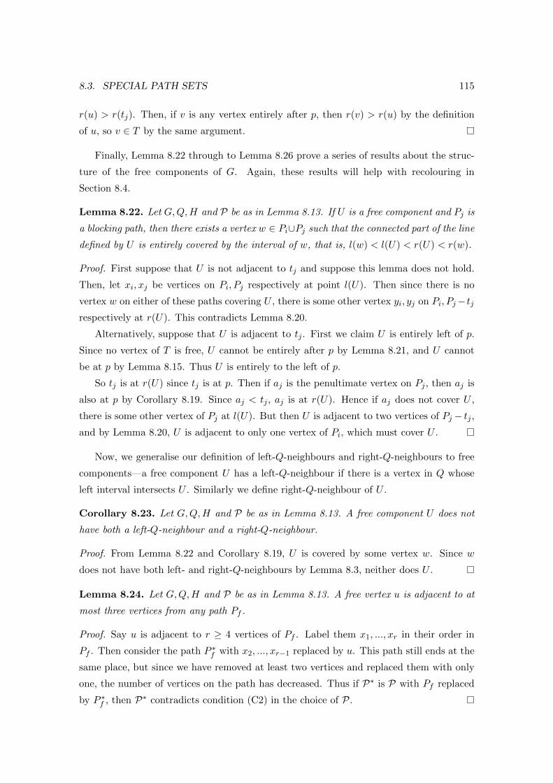
8.3. SPECIAL PATH SETS 115
r(u) > r(tj). Then, if v is any vertex entirely after p, then r(v) > r(u) by the definition
of u, so v ∈ T by the same argument.
Finally, Lemma 8.22 through to Lemma 8.26 prove a series of results about the struc-
ture of the free components of G. Again, these results will help with recolouring in
Section 8.4.
Lemma 8.22. Let G,Q,H and P be as in Lemma 8.13. If U is a free component and Pj is
a blocking path, then there exists a vertex w ∈ Pi∪Pj such that the connected part of the line
defined by U is entirely covered by the interval of w, that is, l(w) < l(U) < r(U) < r(w).
Proof. First suppose that U is not adjacent to tj and suppose this lemma does not hold.
Then, let xi, xj be vertices on Pi, Pj respectively at point l(U). Then since there is no
vertex w on either of these paths covering U , there is some other vertex yi, yj on Pi, Pj− tjrespectively at r(U). This contradicts Lemma 8.20.
Alternatively, suppose that U is adjacent to tj . First we claim U is entirely left of p.
Since no vertex of T is free, U cannot be entirely after p by Lemma 8.21, and U cannot
be at p by Lemma 8.15. Thus U is entirely to the left of p.
So tj is at r(U) since tj is at p. Then if aj is the penultimate vertex on Pj , then aj is
also at p by Corollary 8.19. Since aj < tj , aj is at r(U). Hence if aj does not cover U ,
there is some other vertex of Pj at l(U). But then U is adjacent to two vertices of Pj − tj ,and by Lemma 8.20, U is adjacent to only one vertex of Pi, which must cover U .
Now, we generalise our definition of left-Q-neighbours and right-Q-neighbours to free
components—a free component U has a left-Q-neighbour if there is a vertex in Q whose
left interval intersects U . Similarly we define right-Q-neighbour of U .
Corollary 8.23. Let G,Q,H and P be as in Lemma 8.13. A free component U does not
have both a left-Q-neighbour and a right-Q-neighbour.
Proof. From Lemma 8.22 and Corollary 8.19, U is covered by some vertex w. Since w
does not have both left- and right-Q-neighbours by Lemma 8.3, neither does U .
Lemma 8.24. Let G,Q,H and P be as in Lemma 8.13. A free vertex u is adjacent to at
most three vertices from any path Pf .
Proof. Say u is adjacent to r ≥ 4 vertices of Pf . Label them x1, ..., xr in their order in
Pf . Then consider the path P ∗f with x2, ..., xr−1 replaced by u. This path still ends at the
same place, but since we have removed at least two vertices and replaced them with only
one, the number of vertices on the path has decreased. Thus if P∗ is P with Pf replaced
by P ∗f , then P∗ contradicts condition (C2) in the choice of P.

116 CHAPTER 8. CIRCULAR ARC GRAPHS
Lemma 8.25. Let G,Q,H and P be as in Lemma 8.13. If a free vertex u is adjacent to
distinct vertices x, y, z ∈ Pf for some Pf , where x, y, z is the order of the vertices in the
path, then x and y are both at l(u).
Proof. Some vertex in Pf is at l(u) and some vertex in Pf is at r(u). Since u is adjacent
to only x, y, z ∈ Pf , then x is at l(u) and z is at r(u). If y is not at l(u), then construct
P ∗f from Pf by replacing y with u. Now P ∗f is still a path and it ends at the same place
as before, but l(u) < l(y), contradicting (C3) in the choice of P.
Lemma 8.26. Let G,Q,H and P be as in Lemma 8.13. A free component U has a
right-Q-neighbour.
Proof. Let u be the vertex of U such that r(u) = r(U). The free component U has a
right-Q-neighbour if and only if u has a right-Q-neighbour, so suppose u does not. Thus
by Lemma 8.4 u has k right-only-H-neighbours. By our choice of u, there are no free
vertices other than u at r(u). Hence all of these k vertices are path vertices.
We claim that for each Pf , there is at most one vertex of Pf which is a right-only-H-
neighbour of u. By Lemma 8.24, |N(u) ∩ Pf | ≤ 3. If |N(u) ∩ Pf | = 1, then this vertex
must be at l(u) and r(u), so it is not a right-only-H-neighbour. If |N(u) ∩ Pf | = 2, then
one of these two vertices is at l(u), so there is at most one right-only-H-neighbour of u
in Pf . Finally |N(u) ∩ Pf | = 3, then by Lemma 8.25, two of these vertices are at l(u), so
again Pf contributes at most one right-only-H-neighbour of u.
However, there are only (k−1) paths, and each path contributes at most one right-only-
H-vertex, meaning together there are at most (k−1) vertices, which is a contradiction.
All of these lemmas together give enough of an idea of the structure of G, forcing
enough non-adjacency amongst the vertices to allow us to determine a colouring of G with
less than χ(G) colours.
8.4 Colouring G
Given all the facts we have proven about our graph, we will now show how to colour G
with less that χ(G) = L(G) + k colours, proving that there are no counterexamples. We
will colour the graph in three parts.
First, we colour the clique Q with L colours, such that the vertex qi is coloured i.
Then, we colour the vertices of our special path set P and the remaining vertices of T .
Finally we colour the free vertices. Call this colouring c. For X ⊂ V (G), c(X) will denote
the set of colours assigned to the vertices in X.

8.4. COLOURING G 117
For f ∈ 1, . . . , k− 1, define τf = Pf ∪ tf . If Pf is finished, then τf = Pf . If not, then
τf can be thought of as a path from sf to tf with the final edge missing. We shall now
colour all of the τf .
We want to define (k− 1) disjoint sets of colours Ek−1, . . . , E1, where Ef is the palette
for τf , that is, a set of colours we shall allow use of for τf . By doing this, we ensure that
there can be no monochromatic edge from a vertex in one path to a vertex in another—the
sets of colours we use for each path is different.
Recall that Sf = q1, . . . qf and Tf = q′L, . . . q′L−(k−1)+f. Let A := c(Sk−1) and
B := c(T1). Note that |A| = |B| = (k − 1).
Construct Ek−1, . . . , E1 in that order by the following algorithm. A colour in some Ef
is said to be used.
Say we are constructing Ef .
• Now f ∈ A. If f ∈ B, then set Ef = f, αf, where αf is a new colour. Say Ef has
Type 1.
Otherwise f /∈ B. Then select a colour from c(Tf ) that has not been used before by any
palette, and call it bf . (In Lemma 8.27 below, we prove that this is always possible.) Since
Tf ⊆ T1, we have bf ∈ B.
• If bf ∈ A, then set Ef = bf , αf, where αf is a new colour. Say Ef has Type 2.
• Finally, if f /∈ B and bf /∈ A, then let Ef = f, αf , bf, where αf is a new colour.
Say Ef has Type 3.
We have used (k − 1) new colours α1, . . . , αk−1. However, we need to ensure that the
above algorithm constructs well-defined sets of distinct colours.
Lemma 8.27. Let G be the vertex-minimum counterexample to Theorem 1.12, let Q be
the set of vertices at a point of maximum load q and let H := G −Q. Let P be a special
path set chosen with respect to (C1),(C2) and (C3). It is possible to construct a set of
palettes as described above, and these palettes are pairwise disjoint.
Proof. It is sufficient to prove the following stronger statement by induction: For all
f ∈ (k − 1), . . . 1, the sets Ek−1, . . . , Ef are well-defined and pairwise disjoint, andk−1⋃j=f
Ej contains (k − f) colours in B, and 1, . . . , f − 1 ∩ (k−1⋃j=f
Ej) = ∅.
First we show it is possible to construct Ek−1, the base case:
• Note that (k − 1) ∈ A. If (k − 1) ∈ B, then Ek−1 = (k − 1), αk−1. So far we have
used one colour from B, and we have not used 1, . . . , (k − 2).
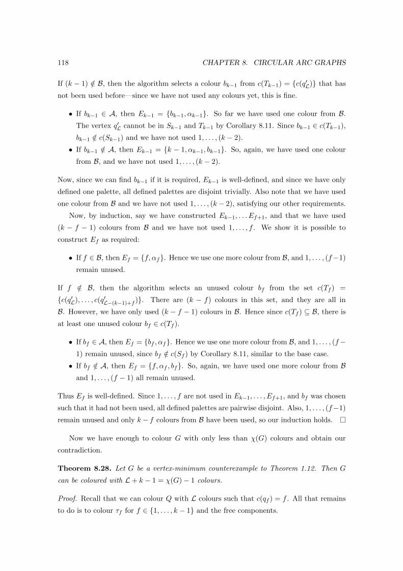
118 CHAPTER 8. CIRCULAR ARC GRAPHS
If (k − 1) /∈ B, then the algorithm selects a colour bk−1 from c(Tk−1) = c(q′L) that has
not been used before—since we have not used any colours yet, this is fine.
• If bk−1 ∈ A, then Ek−1 = bk−1, αk−1. So far we have used one colour from B.
The vertex q′L cannot be in Sk−1 and Tk−1 by Corollary 8.11. Since bk−1 ∈ c(Tk−1),bk−1 /∈ c(Sk−1) and we have not used 1, . . . , (k − 2).
• If bk−1 /∈ A, then Ek−1 = k − 1, αk−1, bk−1. So, again, we have used one colour
from B, and we have not used 1, . . . , (k − 2).
Now, since we can find bk−1 if it is required, Ek−1 is well-defined, and since we have only
defined one palette, all defined palettes are disjoint trivially. Also note that we have used
one colour from B and we have not used 1, . . . , (k − 2), satisfying our other requirements.
Now, by induction, say we have constructed Ek−1, . . . Ef+1, and that we have used
(k − f − 1) colours from B and we have not used 1, . . . , f . We show it is possible to
construct Ef as required:
• If f ∈ B, then Ef = f, αf. Hence we use one more colour from B, and 1, . . . , (f−1)
remain unused.
If f /∈ B, then the algorithm selects an unused colour bf from the set c(Tf ) =
c(q′L), . . . , c(q′L−(k−1)+f ). There are (k − f) colours in this set, and they are all in
B. However, we have only used (k − f − 1) colours in B. Hence since c(Tf ) ⊆ B, there is
at least one unused colour bf ∈ c(Tf ).
• If bf ∈ A, then Ef = bf , αf. Hence we use one more colour from B, and 1, . . . , (f−1) remain unused, since bf /∈ c(Sf ) by Corollary 8.11, similar to the base case.
• If bf /∈ A, then Ef = f, αf , bf. So, again, we have used one more colour from Band 1, . . . , (f − 1) all remain unused.
Thus Ef is well-defined. Since 1, . . . , f are not used in Ek−1, . . . , Ef+1, and bf was chosen
such that it had not been used, all defined palettes are pairwise disjoint. Also, 1, . . . , (f−1)
remain unused and only k− f colours from B have been used, so our induction holds.
Now we have enough to colour G with only less than χ(G) colours and obtain our
contradiction.
Theorem 8.28. Let G be a vertex-minimum counterexample to Theorem 1.12. Then G
can be coloured with L+ k − 1 = χ(G)− 1 colours.
Proof. Recall that we can colour Q with L colours such that c(qf ) = f . All that remains
to do is to colour τf for f ∈ 1, . . . , k − 1 and the free components.

8.4. COLOURING G 119
Firstly we colour τk−1, ..., τ1 using the sets Ek−1, ..., E1 we constructed in Lemma 8.27.
We claim we can colour each τf with the colours of Ef without creating a monochromatic
edge.
First note that since the colours of the palettes are pairwise disjoint, there will be no
monochromatic edge between a vertex of τf and τg for f 6= g, and since the paths are
induced, there will be no monochromatic edge inside τf as long as we ensure there are no
monochromatic edges between consecutive vertices on τf . The only thing to be careful of
is monochromatic edges between τf and Q.
Say Ef has Type 1. Note we can use αf for any vertex of τf since it is a new colour,
that is, a colour not used by Q. We now show that f can be used for any vertex other than
tf . Since f ∈ c(Sf ), the left interval of the vertex qf does not reach l(sf ) by Lemma 8.10,
and since f ∈ B, the right interval of qf does not reach r(t1). Since there is only one
vertex of T in τf , qf intersects only one vertex of this set. Thus, τf can be coloured by
assigning tf the colour αf , and alternating between f and αf from right to left along the
path.
Say Ef has Type 2. This case is very similar to the previous one; αf is available for
any vertex, and bf is available for any vertex other than sf , by the mirror of the previous
argument. Colour sf by αf and alternate bf and αf along the rest of the path from left
to right.
Say Ef has Type 3. Partition τf into two subpaths τ1f , the vertices of τf without qf
as a right-Q-neighbour, and τ2f , the remaining vertices of τf that do have qf as a right-Q-
neighbour. Now the vertices of τ1f can all use either αf or f , since they do not intersect
the right interval of qf by definition, and they do not intersect the left interval of qf by
Lemma 8.10. Since the vertices of τ2f have a right-Q-neighbour they do not have a left-Q-
neighbour by Lemma 8.3. Hence none of these vertices are adjacent to the left interval of
the vertex of Q coloured bf , and since bf ∈ c(Tf ), none are adjacent to the right interval
of this Q-vertex by Lemma 8.10. Hence we can use bf or αf for any vertex of τ2f . So
colour τ1f such that the last vertex has colour f , that is, colour it f and alternate αf , f
back towards sf , and colour the first vertex of τ2f by αf and alternate bf , αf from left to
right along τ2f .
Hence we can colour each τf as required. So far we have used L + k − 1 colours. We
need to colour the rest of the graph without using any new colours. Only the free vertices
remain. Let U be a free component. Then we claim we can colour U with the existing
colours.
By Lemma 8.26, U has a right-Q-neighbour, and by Corollary 8.23 it has no left-Q-
neighbour. We shall colour the vertices of U by traversing the component from right to

120 CHAPTER 8. CIRCULAR ARC GRAPHS
left, and colouring a vertex u when we reach its right endpoint, with any available colour.
It suffices to show that when we come to colour u that one of the L + k − 1 colours is
not assigned to a vertex adjacent to u. Since U has no left-Q-neighbour, neither does u.
Thus, if there is a Q-vertex adjacent to u, it is at r(u). Similarly, by the order in which
we colour the free vertices, any coloured free vertex in the neighbourhood of u is at r(u).
So if a colour d appears in the neighbourhood of u but not on a vertex at r(u), then it
must appear on a path vertex.
We claim that for a path Pf , there is at most one colour on a vertex in Pf ∩ N(u)
that is not at r(u). For each path Pf , there is at least one vertex of that path at r(u), so
there is at least one colour of c(Pf ∩ N(u)) at r(u). Hence, if |c(Pf ∩ N(u))| ≤ 2, there
is at most one colour of c(Pf ∩ N(u)) not at r(u), as required. Since Pf ⊆ τf , and τf is
coloured with Ef , we have |c(Pf ∩ N(u))| ≤ |Ef |. Hence if |Ef | = 2 (that is, if Ef has
Type 1 or Type 2), our claim holds.
Otherwise, |Ef | = 3, and Ef has Type 3. When we coloured τf with three colours,
we actually 2-coloured each of the two subpaths of τf . Hence if N(u) only intersects
one subpath of τf , then |c(Pf ∩ N(u))| ≤ 2, and we get the same result as above. If
|c(Pf ∩ N(u))| = 3, then N(u) contains vertices from both subpaths. By Lemma 8.24,
|Pf ∩N(u)| ≤ 3, so |c(Pf ) ∩N(u)| = 3 and N(u) contains either one vertex from τ1f and
two from τ2f , or vice versa. In the first case, c(Pf ∩ N(u)) = f, αf , bf. Let the three
vertices of Pf ∩N(u) be x, y, z by their order in Pf . By Lemma 8.25, x and y are at l(u),
and z is at r(u). If y is also at r(u), then we have only one colour of this set not at r(u).
Otherwise, r(y) < r(u) and thus any right-Q-neighbour of y is a right-Q-neighbour of u.
Since y ∈ τ2f , y has qf ∈ Q as a right-Q-neighbour where c(qf ) = f . But then, f is at
r(u), so again there is only one colour of c(Pf ∩ N(u)) not at r(u). In the second case,
c(Pf ∩N(u)) = αf , f, αf, so |c(Pf ∩N(u))| = 2, and our claim holds.
Now, there are (k − 1) paths, and for each path there is at most one colour on that
path not at r(u). Since these are the only colours not at r(u), there are only (k−1) colours
adjacent to u that are not at r(u). There are at most (L − 1) colours at r(u) since L is
the maximum load. Thus there are at most (L− 1) + (k− 1) = L+ k− 2 colours adjacent
to u. We are colouring with L+ k− 1 colours, so there is always a colour free for u. Thus
our claim holds.
Thus, we can colour G with only L+ k − 1 colours, which contradicts χ(G) = L+ k.
This completes the proof of Theorem 1.12.

8.5. EXTENSIONS 121
8.5 Extensions
The question remains as to whether Theorem 1.12 can be improved, either by removing
the −1, and thus proving Hadwiger’s Conjecture for circular arc graphs when β(G) > 3,
or by removing the requirement on the cover number.
We believe that it should be possible to prove that had(G) ≥ χ(G) whenever G is
a circular arc graph with β(G) > 3, and that this should be able to be proven using
techniques similar to those found in this chapter. Note the following facts. A special path
set can be expanded to contain k paths rather than k−1 paths without too much trouble.
All of the important results about the nature of special path sets still hold if we make this
adjustment. However, there are some issues with the colouring arguments that need to
be fixed. For example, if we place a new colour in each palette E1, . . . , Ek, then there are
k new colours. Together with the L colours of Q, this give χ(G) colours in total, which
does not give the improvement we require. Our initial attempts to fix this issue involved
colouring one of the paths with only existing colours, possibly using the fact that at least
one of the paths is unfinished. If Pf is unfinished, then τf is a path with an edge missing,
which should be easier to colour than a normal path.
On the other hand, proving had(G) ≥ χ(G) when β(G) ≤ 3 is likely to be much harder.
First note that the assumption β(G) > 3 is used repeatedly in the proofs of this chapter,
and there is no obvious way to get similar results without this assumption. It is likely
that when β(G) ≤ 3, the constructed minor will need to contain two sets of paths, rather
than a clique and a single special path set. Note, however, that if β(G) = 1, then G
contains a dominating vertex, a vertex adjacent to all other vertices. A vertex minimum
counterexample does not contain such a vertex, since adding a dominating vertex increases
both the chromatic number and the Hadwiger number by 1. Thus removing such a vertex
lowers both parameters by 1, and gives a smaller counterexample. Thus we would only
need to prove the conjecture when β(G) ∈ 2, 3.

122 CHAPTER 8. CIRCULAR ARC GRAPHS

Chapter 9
Linkages in Interval Graphs
9.1 Introduction
Recall that there is some slight overlap in terminology between two different concepts
of “linked”. In this chapter, we shall not use the concept of linkedness presented in
Chapter 2, so there should be no confusion. Recall 2k distinct vertices s1, . . . , sk, t1, . . . , tk
can be linked if there exists a set of k pairwise vertex disjoint paths P1, . . . , Pk such that
Pi starts at si and ends at ti. The paths P1, . . . , Pk are called a linkage. For a graph G,
if |V (G)| ≥ 2k and if any 2j distinct vertices (where j ≤ k) can be linked, then we say
the graph G is k-linked . (Note that if any 2k distinct vertices can be linked, then so can
any 2j distinct vertices for j < k.) We call the vertices s1, . . . , sk sources and t1, . . . , tk
targets.
The power of a path, P kn , is the graph formed by taking the n-vertex path and adding
edges between any two vertices u, v where the distance d(u, v) ≤ k. That is, if we label the
vertices of the path 1, . . . , n, then there is an edge between i and j whenever |i− j| ≤ k.
We shall always label the vertices in this fashion, and we say vertices are left or right
of each other with respect to this labelling. It is clear that P kn is k-connected whenever
n > k. The graph P kn is the interval graph of [i, i + k] : 1 ≤ i ≤ n. (Given that no
interval is completely covered by another, P kn is a proper interval graph.)
The interval graphs are a subset of the chordal graphs. To see this, take a cycle of
length at least 4 and consider the intervals of this cycle in the real line. Let v be the
vertex with the leftmost right endpoint; v has two neighbours in the cycle, but they are
both at the right endpoint of v and this forces a triangle as an induced subgraph of the
cycle. Thus every cycle of length at least 4 has a chord. Recall the following linkage result
for chordal graphs.
Lemma 9.1 (Bohme et al. [9]). If G is a (2k − 1)-connected chordal graph, then G is
123

124 CHAPTER 9. LINKAGES IN INTERVAL GRAPHS
k-linked.
We now provide an alternate proof of Lemma 9.1.
Proof. As discussed in Section 2.4, if G is a chordal graph, then it is possible to find a tree
decomposition T of G such that every bag of the tree decomposition is a clique. Since G is
(2k− 1)-connected, for any two adjacent bags X,Y of T , it follows that |X ∩ Y | ≥ 2k− 1,
since the set X ∩ Y is a cut-set. Similarly, any cut set must contain X ∩ Y for some pair
of adjacent bags X,Y ; otherwise it is possible to find a path in G between any pair of
vertices x, y by taking vertices along the path in T between a bag containing x and a bag
containing y.
Perform induction on k ≥ 1. The base case is clear since a 1-connected graph is 1-
linked. Now consider the case for general k. Given 2k distinct vertices s1, . . . , sk, t1, . . . , tk,
let G′ := G−s2, . . . , sk, t2, . . . , tk. Since G is (2k−1)-connected and only 2(k−1) = 2k−2
vertices have been deleted, the graph G′ is connected. Let P1 be an induced path from
s1 to t1 in G′. The path P1 is also an induced path from s1 to t1 in G which avoids
s2, . . . , sk, t2, . . . , tk. Consider G−P1. Since P1 is induced, it contains at most two vertices
in every bag of T , or else P1 contains a triangle. Hence G−P1 is (2k−3)-connected, since
deleting P1 deleted at most two vertices from X ∩ Y for any pair of adjacent bags X,Y .
Since 2k − 3 = 2(k − 1) − 1, the graph G − P1 is (k − 1)-linked by induction. Thus, let
P2, . . . , Pk be the linkage for s2, . . . , sk, t2, . . . , tk in G− P1. Thus the set P1, P2, . . . , Pk is
the required linkage for s1, . . . , sk, t1, . . . , tk in G.
We now show that Lemma 9.1 is tight, even for powers of a path. (Bohme et al. proved
a similar result, but not in this fashion.) Consider P 2k−23k−1 ; it is sufficient to show that this
graph is not k-linked. Let si = i and ti = 2k − 1 + i for 1 ≤ i ≤ k. Note that si is not
adjacent to ti for any choice of i. Thus each path from si to ti contains at least three
vertices. However, k pairwise vertex disjoint paths, each containing at least three vertices
requires a total of at least 3k vertices. Hence, P 2k−23k−1 is not k-linked.
This above example can be extended to powers of paths with n > 3k − 1 as long as
we ensure our choice of sources and targets are close to one another (that is, they induce
a subgraph that is a power of a path of length 3k − 1).
Before proving Theorem 1.13, we prove a more powerful result for the class of powers
of a path.

9.2. “SELECTION SORT” PATHS IN THE POWER OF A PATH 125
9.2 “Selection Sort” Paths in the Power of a Path
Consider the power of a path P k+rn . We desire to show this graph is something like k-
linked for a small integer r > 0. In order to do this, we need to restrict the sources and the
targets, otherwise this is impossible. First, given any source-target pair si, ti, we declare
that the vertex on the left will always be the source, and the vertex on the right will always
be the target. More drastically, we need to ensure that the minimum distance between
any source si and target tj is at least kr . By ensuring that the sources and targets are “far
apart”, there is enough “room” to be able to organise the paths such that each reaches
the correct target. Also note that this restriction ensures that the example proving the
tightness of Lemma 9.1 is not an obstruction to this alternate result.
Lemma 9.2. Let s1, . . . , sk, t1, . . . , tk be distinct vertices in the graph P k+rn (with r > 0)
such that si is left of ti for all i, and such that the distance between any source and any
target in P k+rn is at least kr . Then s1, . . . , sk, t1, . . . , tk can be linked.
Given the restrictions in Lemma 9.2, note the following. Say si is the rightmost source
and tj is the leftmost target. Now the distance between si and tj is at least kr . (In fact,
that the distance between si and tj is at least kr is sufficient to prove all other sources and
targets are far enough apart.) Given that P k+rn is k-connected, it is possible to take paths
starting at s1, . . . , sk − si and ending at the k − 1 vertices immediately left of si, that
do not use any vertex right of si. (This last part follows from the fact that we can ensure
these paths are actually paths in P kn , and the k consecutive vertices ending at si are a cut
set of P kn .)
s3b b b b b b
s2
b b b b
s1b b b b b b b b b b b
sik − 1
Figure 9.1: It is sufficient to take paths from the sources to the k− 1 vertices immediately
left of si, and then take paths from those k vertices (that is, including si) to the correct
corresponding targets.
A similar fact holds concerning the vertices immediately right of tj . Thus, if we can
link the k vertices ending at si with the k vertices starting at tj (for any possible choice
of the k pairs), then this is sufficient to prove Lemma 9.2. So the following lemma is
sufficient.

126 CHAPTER 9. LINKAGES IN INTERVAL GRAPHS
Lemma 9.3. Let n ≥ 2k, and let s1, . . . , sk be the first k vertices of the graph P k+rn (in any
order) and t1, . . . , tk be the last k vertices (again in any order). If r > 0 and the distance
between the rightmost source and the leftmost target is at least kr , then s1, . . . , sk, t1, . . . , tk
can be linked.
We can actually go further than this. Partition the vertices of P k+rn into blocks of size
k, such that the first k vertices form the first block, the second k vertices the second, and
so on. Note that the first block contains exactly the sources; call this the source block,
and label it 0. Label the subsequent blocks consecutively. All vertices in the jth block
are distance j from the final source. Whenever n 6≡ 0 mod k, the targets will not all be
in the same block, and will be split over two consecutive blocks. Given that the distance
between sources and targets is at least dkr e, it follows that the first block that contains
targets will be labelled dkr e or higher. From the targets in the second target block take
the set of edges into the corresponding non-target vertices of the first target block. This
is possible given that the targets and corresponding non-targets are distance k in Pn. If
we construct the correct paths from the sources into the vertices of the first target block,
then those paths with the above edges added give the desired linkage.
Also note all vertices of the first target block are still at a distance of at least dkr e from
the sources. If the distance is greater than dkr e, then take a set of edges from each vertex
in the first target block to the corresponding vertex in the previous block. If we construct
a set of paths from the sources to the block before the first target block, then we can add
these edges to get the desired linkage. By doing this repeatedly, we can ensure we only
need paths from the source block to the block dkr e.Finally note that since both sources and targets appear in any order, we can permute
the labels of the targets so that they appear in the obvious order (that is, t1 before t2
and so on), as long as we perform the corresponding permutation on the sources. Taken
together, this means it is sufficient to prove Lemma 9.4 in order to prove Lemma 9.2.
Lemma 9.4. Consider the graph P k+rn where r > 0 and n = dkr ek+k. Label the last k ver-
tices t1, . . . , tk, such that tk is the last vertex, tk−1 the second last and so on. Label the first
k vertices s1, . . . , sk. Regardless of the order of s1, . . . , sk, the vertices s1, . . . , sk, t1, . . . , tk
can be linked.
Proof. Recall that we have partitioned the vertices of P k+rn into dkr e+1 blocks of k vertices
each, labelled from 0 to dkr e. Each path from a source to a target will intersect each block
exactly once. Label each vertex of a block by one of p1, . . . , pk to denote which path it is
on. Label each source si with pi. As long as

9.2. “SELECTION SORT” PATHS IN THE POWER OF A PATH 127
• the vertex labelled with pi in one block is adjacent to the vertex labelled pi in the
previous block, and
• each ti is labelled pi,
then the required linkage has been constructed.
Let 1 ≤ j ≤ dkr e. In the jth block, label the first minjr, k vertices by p1, . . . , pminjr,k
in that order, and call this set of labels the first subset. When minjr, k = jr, we may
still have the labels pjr+1, . . . , pk to place. Place these remaining labels on the remaining
k−jr vertices of the jth block in the same order as the labels appear in the 0th block. Call
this the second subset. The final block is labelled dkr e, and so for this block all vertices are
labelled by the first subset, and so each ti is labelled by pi. Hence this labelling satisfies
the second bulleted requirement above.
It remains to check that the first requirement holds. Consider the jth block. It is easy
to see that the vertices labelled p1, . . . , p(j−1)r are adjacent to the equivalently labelled
vertices in the previous block. (In fact, this fact would hold even if the graph was P kn .)
The remaining labels may have appeared on the corresponding vertex in the previous
block, or on a vertex at most r vertices before the corresponding vertex, given the r new
labels in the first subset. However, in P k+rn each vertex is adjacent to k+ r vertices before
it in the ordering, so the first bulleted requirement holds. This proves the lemma.
We call these “selection sort” paths since if r = 1, then the labels in each block appear
to be undergoing selection sort—each block in sequence is another pass over the linked
list and another label is placed in the correct position. Finally at the last step, all labels
are in the correct position, and the sources are linked up to the correct targets. When
r > 1, this is equivalent to selection sort with more labels moved at every given step. This
means less steps are required. We need to ensure that the sources and targets are far
enough apart so that “selection sort” has the “time” (by which we mean, the space in the
vertex set) to run completely. Given that each vertex is adjacent to k+ r vertices after it
in the ordering, a label can only be moved up by at most r places, so this process cannot
obviously be improved. Because of this, Lemma 9.4 is best possible in the sense that if
r = 0 and the ordering of the sources is not simply s1, . . . , sk, then it is impossible to
link the sources and targets; as we try to build the paths from the sources to the targets,
sequential vertices in a given path must be corresponding vertices in sequential blocks, or
some other path cannot be extended. However, this means no kind of “rearrangement” is
possible, and as such the sources and the targets will not link up correctly. So we cannot
ensure k-connectivity gives even our weakened version of k-linked.
We discuss a use of this “selection sort” technique in Section 9.4.

128 CHAPTER 9. LINKAGES IN INTERVAL GRAPHS
9.3 Improved Linkages in Interval Graphs
The result of Section 9.2 is of some interest, but it would be far more preferable to extend
Lemma 9.2 to a more general class of graphs. Here we extend a limited version of this
result to the class of interval graphs.
Theorem 1.13. Let G be a d3k2 e-connected interval graph, and let s1, . . . , sk, t1, . . . , tk be
2k pairwise distinct vertices, such that no source si and no target tj are adjacent, and
such that si is left of ti for all i. Then s1, . . . , sk, t1, . . . , tk can be linked.
Note that this is essentially Lemma 9.2 generalised for the interval graph when r = k2 .
Many of the techniques used in the proof of Theorem 1.13 are similar to those used in
Chapter 8. Also note that since si and ti are not adjacent, the requirement that si is left
of ti is unambiguous.
First, we recall the following basic facts about an interval graph G (which are quite
similar to the basic facts about circular arc graphs). Given that every vertex of the
interval graph corresponds to an interval on the real line, we often treat the vertex and
its corresponding interval interchangeably. (Only in rare cases do we need to be more
explicit.) Thus every vertex v has a left endpoint denoted l(v) and a right endpoint denoted
r(v). By perturbing the endpoints of all the intervals, we can ensure that no point is an
endpoint (left or right) of more than one interval. Connected induced subgraphs also have
corresponding intervals on the real line (that is, the union of all the intervals corresponding
to vertices of the subgraph); hence if U is a connected induced subgraph we define l(U) and
r(U) to be its endpoints. If we consider all of the right endpoints of the vertices in G, define
the leftmost of these points to be the start point . Also define the rightmost left endpoint of
a vertex to be the final point . The minimum load `(G) is the minimum number of vertices
at any point between the start and final points. (We make this restriction, otherwise the
minimum load might be 0.) It is well known and easily seen that the minimum load is
equal to the connectivity of G.
Define a special path set P to be a set of paths P1, . . . , Pk in G that satisfy the following
properties.
(P1) P1, . . . , Pk are pairwise vertex-disjoint.
(P2) si ∈ Pi for all i, and tj /∈ Pi when j 6= i.
This is essentially identical to the definition of a special path set in Chapter 8, however
note that there are k (and not (k − 1)) paths in P. If ti ∈ Pi we say that Pi is finished,
otherwise it is unfinished. If all paths are finished, then we say P is itself finished, otherwise
it is unfinished. Let pi be the rightmost point of Pi, for all Pi.

9.3. IMPROVED LINKAGES IN INTERVAL GRAPHS 129
Obviously, if P is finished then it is a linkage, and Theorem 1.13 holds. Otherwise, we
can assume that every special path set is unfinished. Let X ⊆ p1, . . . , pk be the set of
right endpoints from unfinished paths, and let p be the leftmost point in X (note X 6= ∅).Choose P so that
(C1) The point p, as defined above, is as far right as possible.
(C2) Subject to (C1), |V (P1) ∪ · · · ∪ V (Pk)| is minimised.
This choice of P (specifically the definition of p) is different than the choice of P in
Chapter 8. The definition of p is done this way since now we cannot assume that the
sources and the targets form cliques at the start and end of the interval respectively, as
was the case in Chapter 8. Also, the requirement (C3) is no longer required since it was
previously included to assist with colouring, which is not relevant here.
We will prove a contradiction by showing that P can be modified so that p is moved
further to the right, which gives a better choice of P.
Say Pi is the unfinished path such that pi = p, and say Pj is a path (finished or
unfinished) such that pj > p. If replace Pi with a path that is either finished, or unfinished
with a right endpoint further right than p, then p itself has been moved further right. (It
is possible p may no longer refer to the same pi, but the point it refers to will be right of
the old p given that p is leftmost in X.) If, while replacing Pi with this new path, we also
replace Pj with another shorter path, then as long as the right endpoint of the new Pj is
right of the original p, the new p is still further right than the old p. This follows even if
Pj has gone from finished to unfinished. This means we can replace Pi (and perhaps Pj)
in a way that is essentially identical to Chapter 8 in order to construct a better choice of
P. As a result, for many of our basic results we shall simply cite the appropriate previous
result.
Lemma 9.5. Let G be a d3k2 e-connected interval graph, and let s1, . . . , sk, t1, . . . , tk be 2k
distinct vertices, such that no source si and no target tj are adjacent, and such that si
is left of ti for all i. Let P be the special path set chosen with respect to (C1) and (C2).
Then every Pi ∈ P is an induced path, and no vertex of Pi other than si or ti is covered
by any other vertex of Pi.
Proof. This follows from Lemma 8.13. However note a slight weakening—it is possible
that the source or the target on Pi is covered by another vertex. This is because si and ti
are not necessarily at the start and end of the interval.
As before, a vertex of G that is in no path of P and is not a target is called a free
vertex .

130 CHAPTER 9. LINKAGES IN INTERVAL GRAPHS
Lemma 9.6. Let G, s1, . . . , sk, t1, . . . tk, and P be as in Lemma 9.5. Let Pi be the unfin-
ished path such that pi = p. Then there is neither a free vertex nor the vertex ti at p, and
as such ti is right of p.
Proof. The first part of this lemma follows from Lemma 8.15. The second part follows
from the self-evident fact that the unfinished path Pi is not adjacent to ti at any point,
and from the relative positions of si and ti on the real line.
By Lemma 9.5, every path Pj of P is induced, so it follows that at any point on the
real line at most two intervals in Pj are present. If a path Pj contains two vertices at a
point r, we say Pj appears twice at point r. If Pi is the path such that pi = p, then Pi
does not appear twice at point p, since p is the right endpoint of an end vertex of the Pi.
Lemma 9.7. Let G, s1, . . . , sk, t1, . . . tk, and P be as in Lemma 9.5. If Pj appears twice
at point p, then one of the two vertices of Pj at p is the vertex tj.
Proof. This follows from Lemma 8.18.
Now, consider the point p + ε, the point just after p but before the left endpoint of
any other vertex. At p + ε there are at least d3k2 e vertices, since p + ε is left of l(ti) by
Lemma 9.6 and thus left of the final point. Hence at p itself there are at least d3k2 e + 1
vertices. By Lemmas 9.6 and 9.7, all of the vertices at p are on paths of P, and any
path that appears twice at point p includes a target vertex. There must be dk2e+ 1 paths
appearing twice at point p, otherwise there are insufficient vertices at p. Hence there is at
least one target at p, and so no source at p.
If Pi is the unfinished path such that p = pi, then Pi contains at least two vertices
since the vertex at p is not si. Let yi denote the rightmost vertex of Pi such that no target
at p is also at l(yi). We show that such a vertex is well-defined. If v is the vertex of Pi
adjacent to si, then either l(v) is inside si, or it is left of l(si). In either case, any target
at both p and l(v) must be adjacent to si, contradicting our assumption about G. Hence
there exists some vertex of Pi such that there is no target at both its left endpoint and at
p, and so yi is well-defined. It also follows that yi 6= si, so let xi denote the neighbour of
yi in Pi that is before yi in the path.
Recall that a maximal connected induced subgraph of G containing only free vertices,
is called a free component . Denote the free component at l(yi) by U , and say U = ∅ if
there is no such free component. We define the reverse point q to be l(U) if U 6= ∅, or
l(yi) if U = ∅. It is possible that the reverse point is left of the start point; if it is not, we
say it has type 1 and if it is we say it has type 2. When q has type 1, we have a situation
similar to Lemma 8.20, but when q has type 2 our proof is rather different.

9.3. IMPROVED LINKAGES IN INTERVAL GRAPHS 131
Lemma 9.8. Let G, s1, . . . , sk, t1, . . . tk, and P be as in Lemma 9.5. Let q be the reverse
point. Then q does not have type 1.
Proof. Since q is right of the start point and q is the endpoint of some vertex, it follows
that there are at least d3k2 e + 1 vertices at q (for the same reason there are at least that
many at p). By the maximality of U , at most one of these vertices is a free vertex, so it
follows that at least dk2e paths of P appear twice at q. Given that dk2e + 1 paths of Pappear twice at p, it follows that some path Pj appears twice at q and at p. Let Pi be the
path such that p = pi; it follows i 6= j, since Pi does not appear twice at point p. Denote
the vertices of Pj at q by aj , bj such that r(aj) < r(bj). Denote the vertices of Pj at p
by cj , tj such that r(cj) < r(tj). It is possible that bj = cj , but otherwise aj , bj , cj , tj are
pairwise disjoint and r(bj) < r(cj). This follows since there are no targets at both q and
p, by choice of yi and since q ≤ l(yi) < p.
Given this, the path Pj has the form (sj , . . . , aj , bj , . . . , cj , tj). Denote the vertex of
Pi at p by ai. Then Pi has the form (si, . . . , xi, yi, . . . , ai). It is possible that si = xi
and/or yi = ai. Partition these paths into the following subpaths: P 1j := (sj , . . . , aj),
P 2j := (bj , . . . , cj), P
3j := (tj) and P 1
i := (si, . . . , xi), P2i := (yi, . . . , ai).
Consider P 1j ∪ U ∪ P 2
i ∪ P 3j . We can replace Pj with this path which travels from sj
to tj , however, we will also need to replace Pi, otherwise P 2i is contained into two paths
of P. Fortunately, the set P 2j is not longer being used in Pj , and this subpath covers the
real line from q to p, and as such covers l(yi), a point which contains xi. Hence replace Pi
with P 1i ∪ P 2
j .
q p
sib b b b b
xi
yi
b b bai
U
sjb b b
aj
bj
b b b b b b
cj
tj
Pi
Pj
q p
si b b b b bxi
yi
b b b b b b
aiUsjb b b
aj
bj
b b b b
cj
tj
Pi
Pj
Figure 9.2: The subpath P 2j is placed into Pi, and P 2
i is placed into Pj . It may be necessary
to place vertices of U into Pj to maintain connectivity. Note the similarity to Figure 8.2.
The right end of each path remains unchanged except for Pi, and pi ≥ r(ci) > p. Hence
p has been moved further right, contradicting our choice of P.

132 CHAPTER 9. LINKAGES IN INTERVAL GRAPHS
In the proof of Lemma 9.8, we essentially “swap” the middle sections of Pi and Pj in
such a way that Pj is still finished, but Pi is now able to travel further right. This is the
key idea in the proof of Theorem 1.13. However, we also must deal with a few other cases.
Lemma 9.9. Let G, s1, . . . , sk, t1, . . . tk, and P be as in Lemma 9.5. Let q be the reverse
point. Then q does not have type 2.
Proof. In order to prove this, we also define a second reverse point. Let Pi be the unfinished
path such that p = pi. Let the free component at r(xi) be denoted U ′ (and let U ′ = ∅ if
there is no such free component). Then let the second reverse point q′ := r(U ′) (or r(xi)
if U ′ = ∅). Since Pi does not appear twice at p and since there are no free vertices at p,
it follows that q′ < p. As with q in Lemma 9.8, there are dk2e paths appearing twice at q′,
and as such there exists a Pj that appears twice at q′ and p.
Let ai be the vertex of Pi at p and partition the path Pi as in Lemma 9.8: P 1i :=
(si, . . . , xi) and P 2i := (yi, . . . , ai). Given that q is left of the start point, it follows that
P 2i ∪ U covers the entire real line from the start point to p. Hence, since Pj contains a
target at p, it follows that r(sj) < p and as such sj is adjacent to P 2i ∪ U .
If P 1i is adjacent to Pj − sj , then replace Pj with sj ∪ P 2
i ∪ U ∪ tj and Pi with
P 1i ∪ (Pj−sj , tj). In this case p is further right, since the new Pi ends further right than
p due to Pj appearing twice at p.
p
sib b b b b
xi
yi
b b bai
U
sjb b b b b b b b b
tj
Pi
Pj
p
sib b b b b
xi
yib b b b
aiUsj
b b b b b b b b b
tj
Pi
Pj
Figure 9.3: Given that q is left of the start point, it is easy to place P 2i ∪ U into Pj . This
leaves Pj−sj , tj available for Pi. When Pj− sj is adjacent to P 1i , this is sufficient. Also
note the second reverse point is not used in this case.
However, it is possible that P 1i is not adjacent to Pj−sj . This means that l(Pj−sj) >
r(xi), and since sj is at l(Pj − sj), it follows sj is adjacent to some vertex of P 2i . Since
Pj appears twice at q′, the subpath Pj − sj is adjacent to P 1i ∪U ′. Hence replace Pj with

9.3. IMPROVED LINKAGES IN INTERVAL GRAPHS 133
sj ∪P 2i ∪ tj and replace Pi with P 1
i ∪U ′ ∪ (Pj −sj , tj). The point p has once again
been moved further right, contradicting our choice of P.
q′ p
sib b b b b
xi
yi
b b b bai
U ′
sjb b
tj
Pi
Pj
q′ p
sib b b b b
xi
yib b b b
ai
U ′
sj
b b
tj
Pi
Pj
Figure 9.4: Using the second reverse point, it is possible to place P 2i into Pj and then
Pj − sj , tj into Pi, maintaining connectivity with U ′.
Given that reverse point q must exist and have either type 1 or type 2, Lemma 9.8 and
Lemma 9.9 are sufficient to prove that a finished P must exist. This proves Theorem 1.13.
The connectivity requirement in Theorem 1.13 is tight. Let k be even, and
consider G := P3k2−1
n , where n = 2k + 3k2 − 1. Label the vertices (in order)
s1, . . . , sk, a1, . . . , a 3k2−1, t k
2+1, . . . , tk, t1, . . . , t k
2. The graph G is not 3k
2 -connected, and no
si and tj are adjacent, so if we show s1, . . . , sk, t1, . . . , tk cannot be linked, then Theo-
rem 1.13 is tight.
Suppose for the sake of a contradiction there is a linkage P1, . . . , Pk. Each Pi in the
linkage contains si and ti, but all other vertices in Pi are labelled by some aj . Since no
source is adjacent to no target, each Pi contains at least three vertices.
Say there exists some aj adjacent to both si and ti where i ≤ k2 . Now since aj is
adjacent to si, it follows that j ≤ k2 + i − 1. Since aj is adjacent to ti, it follows that
j ≥ k2 + i. So there is no such aj . As a result, each Pi contains four vertices when
i ≤ k2 . Thus the linkage contains at least 3k2 + 4k2 vertices in total, but this is greater than
n = 2k+ 3k2 − 1, the number of vertices in G. Hence s1, . . . , sk, t1, . . . , tk cannot be linked.
Theorem 1.13 is a restricted extension of Lemma 9.2 for the broader class of interval
graphs. We believe that it should be possible to extend the entire lemma, and as such
make the following conjecture.
Conjecture 9.10. Let s1, . . . , sk, t1, . . . , tk be 2k distinct vertices in (k + r)-connected
interval graph G (with r > 0), such that si is left of ti for all i, and such that the distance

134 CHAPTER 9. LINKAGES IN INTERVAL GRAPHS
between any source and any target in G is at least kr . Then s1, . . . , sk, t1, . . . , tk can be
linked.
Our motivation for Theorem 1.13 comes from Theorem 1.12. Recall that given a
circular arc graph, we can delete the vertices at a point and obtain an interval graph.
Constructing a linkage along this interval was a key step in trying to construct a complete
minor in our proof of Theorem 1.12. However, the requirement that source and target
vertices be non-adjacent (or even further apart) essentially forces the cover number of
the circular arc graph, β, to be large. (This is to say, if there is a small vertex cover
of the circular arc graph, then there is probably a short path between any source and
any target, depending on where we “cut” the circle.) As a result of this Conjecture 9.10,
while interesting, would not really assist in Chapter 8. Any attempt to prove Hadwiger’s
Conjecture for circular arc graphs when β is small will require some alternate approach.
Finally, it is also worth asking whether Theorem 1.13 can be extended to the more
general class of chordal graphs. Unfortunately, the answer to this question is no. We
provide a counterexample that is (2k − 2)-connected but not k-linked, even when sources
and targets are not adjacent. (This is essentially a more general example that Lemma 9.1
is tight.)
Given the connection between chordal graphs and treewidth as seen in Section 2.4 and
the proof of Lemma 9.1, we shall exhibit this graph as a tree decomposition. The vertices
of G are exactly the vertices that appear in at least one bag of the tree decomposition,
and E(G) contains all acceptable edges for the tree decomposition—if two vertices share
a bag, then they are adjacent. Recall that as long as every two adjacent bags in the tree
decomposition contain at least 2k− 2 vertices in common, then the chordal graph G that
arises from this tree decomposition is (2k − 2)-connected, since deleting any set of less
than 2k − 2 vertices leaves a vertex present in each pair of adjacent bags which is enough
to ensure connectivity.
Let the underlying tree T be the star with k leaves, such that each edge has been
subdivided k − 1 times. The vertices of G are as follows:
• sources s1, . . . , sk,
• targets t1, . . . , tk,
• a1, . . . , ak−1, called the a-vertices,
• bi1, . . . , bik for all 1 ≤ i ≤ k.
In the bag indexed by the centre node, which we label C, place the vertices
s1, . . . , sk, a1, . . . , ak−1. Denote the path in T from the centre node to the ith leaf as
the ith path. Let Bi denote the bag adjacent to C in the ith path. The bag Bi contains

9.4. HADWIGER NUMBER OF THE POWER OF A CYCLE 135
all vertices of C except si, and also includes vertex bi1. For each subsequent bag on the
ith path, remove a source vertex and add a vertex from bi1, . . . , bik, until the final bag on
the ith path contains a1, . . . , ak−1, bi1, . . . , bik. To this final bag, also add ti. Given the
way we have constructed these bags, it is clear that adjacent bags contain at least 2k − 2
vertices in common. Hence the chordal graph that arises from this tree decomposition is
(2k − 2)-connected.
However, we cannot link each si to ti in this graph G. Note that si does not appear
in any bag along the ith path, and ti only appears at the end of the ith path. Thus any
path from si to ti contains a vertex in C ∩Bi = s1, . . . , sk, a1, . . . , ak−1−si, since this
set of vertices separates the graph such that si and ti are in different components. Given
that this path cannot use another source, it must contain an a-vertex. But there are k
paths, and only (k − 1) a-vertices, and as such we cannot link these sources and targets,
even though they are not adjacent.
9.4 Hadwiger Number of the Power of a Cycle
Recall the kth-power of a cycle Ckn is the graph formed by taking a cycle and adding edges
between any two vertices at distance at most k.
In Chapter 1, we proved a lower bound on had(Ckn) when n ≡ 1 mod k and n ≥ 2k+1.
As promised, we prove a lower bound that is independent of the modulus of n, using the
results of Section 9.2.
Lemma 9.11. If n ≥ k2 + 2k, then had(Ckn) ≥ 2k.
Proof. Label the vertices of the power of the cycle 1, . . . , n clockwise. The graph Ckn −1, . . . , k+1 is isomorphic to the power of a path P kn−k−1. Given Lemma 9.4, we construct
a set of k − 1 paths in P kn−k−1 (and thus in Ckn) from k + 2, . . . , 2k to n − k + 2, . . . , n
respectively. These paths form k − 1 branch sets of the K2k model. (It is clear that
these branch sets are adjacent to each other.) The remaining k + 1 branch sets are
singleton branch sets 1, , . . . , k+1. (Note these vertices form a clique.) Each vertex
i ∈ 1, . . . , k is adjacent to n− k+ i, . . . , n and k+ 2, . . . , k+ i, and as such is adjacent
to every one of the paths. Finally, the vertex k+1 is adjacent to k+2, . . . , 2k+1 and so is
also adjacent to each one of the paths. This gives a complete model with k+1+k−1 = 2k
branch sets, as required.
Note that the above minor is very similar to the minor we attempted to construct in
Chapter 8, but much stronger given what we know about the power of a cycle.

136 CHAPTER 9. LINKAGES IN INTERVAL GRAPHS
Recall we proved in Section 1.4 that pw(Ckn) ≤ 2k. For large n, this means
2k − 1 ≤ had(Ckn)− 1 ≤ tw(Ckn) ≤ pw(Ckn) ≤ 2k.
Thus Lemma 9.11 is almost best possible.

Bibliography
[1] Albertson, M. O., Chappell, G. G., Kierstead, H. A., Kundgen, A., and Ramamurthi,
R. (2004). Coloring with no 2-colored P4’s. Electron. J. Combin., 11 #R26.
[2] Appel, K. and Haken, W. (1976). A proof of the four color theorem. Discrete Math.,
16(2), 179–180.
[3] Atserias, A. (2008). On digraph coloring problems and treewidth duality. European
J. Combin., 29(4), 796–820.
[4] Belkale, N. and Chandran, L. S. (2009). Hadwiger’s conjecture for proper circular
arc graphs. European J. Combin., 30(4), 946–956.
[5] Bellenbaum, P. and Diestel, R. (2002). Two short proofs concerning tree-
decompositions. Combin. Probab. Comput., 11(6), 541–547.
[6] Bodlaender, H. L. (1993). A tourist guide through treewidth. Acta Cybernet., 11(1-
2), 1–21.
[7] Bodlaender, H. L. (1998). A partial k-arboretum of graphs with bounded treewidth.
Theoret. Comput. Sci., 209(1-2), 1–45.
[8] Bodlaender, H. L., Grigoriev, A., and Koster, A. M. C. A. (2008). Treewidth lower
bounds with brambles. Algorithmica, 51(1), 81–98.
[9] Bohme, T., Gerlach, T., and Stiebitz, M. (2008). Ordered and linked chordal graphs.
Discuss. Math. Graph Theory , 28(2), 367–373.
[10] Bollobas, B. and Thomason, A. (1996). Highly linked graphs. Combinatorica, 16(3),
313–320.
[11] Calinescu, G., Fernandes, C., and Reed, B. A. (2003). Multicuts in unweighted
graphs and digraphs with bounded degree and bounded tree-width. J. Algorithms,
48(2), 333–359.
137

138 BIBLIOGRAPHY
[12] Catlin, P. A. (1979). Hajos’ graph-coloring conjecture: variations and counterexam-
ples. J. Combin. Theory Ser. B , 26(2), 268–274.
[13] Chambers, J. (2002). Hunting for Torus Obstructions. M.Sc. thesis, Department of
Computer Science, University of Victoria, Canada.
[14] Chekuri, C. and Chuzhoy, J. (2013). Polynomial bounds for the grid-minor theorem.
arXiv: 1305.6577.
[15] Chudnovsky, M. and Ovetsky Fradkin, A. (2008). Hadwiger’s conjecture for quasi-
line graphs. J. Graph Theory , 59(1), 17–33.
[16] Chudnovsky, M., Reed, B. A., and Seymour, P. D. (2011). The edge-density for K2,t
minors. J. Combin. Theory Ser. B , 101(1), 18–46.
[17] Colin de Verdiere, Y. (1998). Multiplicities of eigenvalues and tree-width of graphs.
J. Combin. Theory Ser. B , 74, 121–146.
[18] Curtis, A., Lin, M. C., McConnell, R., Nussbaum, Y., Soulignac, F. J., Spinrad, J.,
and Szwarcfiter, J. L. (2013). Isomorphism of graph classes related to the circular-
ones property. Discrete Math. Theor. Comput. Sci., 15(1).
[19] DeVos, M., Dvorak, Z., Fox, J., McDonald, J., Mohar, B., and Scheide, D. (2014).
A minimum degree condition forcing complete graph immersion. Combinatorica, in
print .
[20] Di Giacomo, E., Didimo, W., Liotta, G., and Montecchiani, F. (2012). h-Quasi
planar drawings of bounded treewidth graphs in linear area. In Proceedings of the
38th International Conference on Graph-Theoretic Concepts in Computer Science,
WG’12, pages 91–102, Berlin. Springer-Verlag.
[21] Dıaz, J., Serna, M., and Wormald, N. (2007). Bounds on the bisection width for
random d-regular graphs. Theoret. Comput. Sci., 382(2), 120–130.
[22] Diestel, R. (2000). Graph Theory . Springer.
[23] Diestel, R., Jensen, T. R., Gorbunov, K. Y., and Thomassen, C. (1999). Highly
connected sets and the excluded grid theorem. J. Combin. Theory Ser. B , 75(1),
61–73.
[24] Dirac, G. A. (1952). A property of 4-chromatic graphs and some remarks on critical
graphs. J. London Math. Soc., 27, 85–92.

BIBLIOGRAPHY 139
[25] Dujmovic, V., Morin, P., and Wood, D. R. (2005). Layout of graphs with bounded
tree-width. SIAM J. Comput., 34(3), 553–579.
[26] Dujmovic, V., Harvey, D. J., Joret, G., Reed, B. A., and Wood, D. R. (2013). A
linear-time algorithm for finding a complete graph minor in a dense graph. SIAM
J. Discrete Math., 27(4), 1770–1774.
[27] Erdos, P. (1959). Graph theory and probability. Canad. J. Math., 11, 34–38.
[28] Erdos, P., Ko, C., and Rado, R. (1961). Intersection theorems for systems of finite
sets. Quart. J. Math. Oxford Ser. (2), 12, 313–320.
[29] Flum, J. and Grohe, M. (2006). Parameterized Complexity Theory . Texts in Theo-
retical Computer Science. An EATCS Series. Springer.
[30] Fox, J. (2011). Constructing dense graphs with sublinear Hadwiger number. J.
Combin. Theory Ser. B (to appear). arXiv: 1108.4953.
[31] Frankl, P. (1984). A new short proof for the Kruskal-Katona theorem. Discrete
Math., 48(2-3), 327–329.
[32] Fulkerson, D. R. and Gross, O. A. (1965). Incidence matrices and interval graphs.
Pacific J. Math., 15, 835–855.
[33] Ganian, R., Hlineny, P., Langer, A., Obdrzalek, J., Rossmanith, P., and Sikdar,
S. (2014). Lower bounds on the complexity of MSO1 model-checking. J. Comput.
System Sciences, 80(1), 180–194.
[34] Gavril, F. (1974a). Algorithms on circular-arc graphs. Networks, 4(4), 357–369.
[35] Gavril, F. (1974b). The intersection graphs of subtrees in trees are exactly the
chordal graphs. J. Combin. Theory Ser. B , 16, 47–56.
[36] Gerbner, D., Lemons, N., Palmer, C., Patkos, B., and Szecsi, V. (2012). Almost
intersecting families of sets. SIAM. J. Discrete Math., 26(4), 1657–1669.
[37] Gerbner, D., Lemons, N., Palmer, C., Palvolgyi, D., Patkos, B., and Szecsi, V.
(2013). Almost cross-intersecting and almost cross-Sperner pairs of families of sets.
Graph. Combin., 29, 489–498.
[38] Grippo, L. N. and Safe, M. D. (2012). On circular-arc graphs having a model with
no three arcs covering the circle. In Anais do XLIV Simposio Brasileiro de Pesquisa
Operacional , pages 4093–4104. arXiv: 1402.2641.

140 BIBLIOGRAPHY
[39] Grohe, M. and Marx, D. (2009). On tree width, bramble size, and expansion. J.
Combin. Theory Ser. B , 99(1), 218–228.
[40] Hadwiger, H. (1943). Uber eine Klassifikation der Streckenkomplexe. Vierteljschr.
Naturforsch. Ges. Zurich, 88, 133–142.
[41] Halin, R. (1976). S-functions for graphs. J. Geometry , 8(1-2), 171–186.
[42] Harvey, D. J. and Wood, D. R. (2012). Treewidth of line graphs. arXiv: 1210.8205.
[43] Harvey, D. J. and Wood, D. R. (2013). Parameters tied to treewidth.
arXiv: 1312.3401.
[44] Harvey, D. J. and Wood, D. R. (2014a). Treewidth of the Kneser graph and the
Erdos-Ko-Rado theorem. Electron. J. Combin., 21(1), P1.48.
[45] Harvey, D. J. and Wood, D. R. (2014b). Treewidth of the line graph of a complete
graph. J. Graph Theory (to appear).
[46] Jensen, T. R. and Toft, B. (1995). Graph Coloring Problems. John Wiley.
[47] Jung, H. A. (1970). Eine Verallgemeinerung des n-fachen Zusammenhangs fur
Graphen. Math. Ann., 187, 95–103.
[48] Karapetjan, I. A. (1980). Coloring of arc graphs. Akad. Nauk Armyan. SSR Dokl.,
70(5), 306–311.
[49] Katona, G. O. H. (1968). A theorem of finite sets. In Theory of Graphs (Proc.
Colloq., Tihany, 1966), pages 187–207. Academic Press, New York.
[50] Katona, G. O. H. (1972). A simple proof of the Erdos-Chao Ko-Rado theorem. J.
Combin. Theory Ser. B , 13, 183–184.
[51] Kawarabayashi, K. (2007). On the connectivity of minimum and minimal coun-
terexamples to Hadwiger’s Conjecture. J. Combin. Theory Ser. B , 97(1), 144 –
150.
[52] Kawarabayashi, K. and Kobayashi, Y. (2012). Linear min-max relation between
the treewidth of H-minor-free graphs and its largest grid minor. In 29th Interna-
tional Symposium on Theoretical Aspects of Computer Science, volume 14 of LIPIcs.
Leibniz Int. Proc. Inform., pages 278–289. Schloss Dagstuhl. Leibniz-Zent. Inform.,
Wadern.

BIBLIOGRAPHY 141
[53] Kawarabayashi, K. and Mohar, B. (2007). Some recent progress and applications in
graph minor theory. Graphs Combin., 23(1), 1–46.
[54] Kawarabayashi, K., Kostochka, A. V., and Yu, G. (2006). On sufficient degree
conditions for a graph to be k-linked. Combin. Probab. Comput., 15(5), 685–694.
[55] Kawarabayashi, K., Kobayashi, Y., and Reed, B. A. (2012). The disjoint paths
problem in quadratic time. J. Combin. Theory Ser. B , 102(2), 424–435.
[56] Kneser, M. (1955). Aufgabe 360. Jahresber. Deutsch. Math.-Verein., 58:27.
[57] Kostochka, A. V. (1982). The minimum Hadwiger number for graphs with a given
mean degree of vertices. Metody Diskret. Analiz., (38), 37–58.
[58] Kostochka, A. V. (1984). Lower bound of the Hadwiger number of graphs by their
average degree. Combinatorica, 4(4), 307–316.
[59] Kostochka, A. V. and Prince, N. (2008). On Ks,t-minors in graphs with given average
degree. Discrete Math., 308(19), 4435–4445.
[60] Kostochka, A. V. and Prince, N. (2012). On Ks,t-minors in graphs with given average
degree, II. Discrete Math., 312(24), 3517–3522.
[61] Kreutzer, S. (2012). On the parameterized intractability of monadic second-order
logic. Log. Methods Comput. Sci., 8(1), 1:27, 35.
[62] Kreutzer, S. and Tazari, S. (2010a). Lower bounds for the complexity of monadic
second-order logic. In Proc. 25th Annual IEEE Symposium on Logic in Computer
Science (LICS ’10), pages 189–198. IEEE.
[63] Kreutzer, S. and Tazari, S. (2010b). On brambles, grid-like minors, and parameter-
ized intractability of monadic second-order logic. In Proc. 21st Annual ACM-SIAM
Symposium on Discrete Algorithms, pages 354–364. SIAM.
[64] Kruskal, J. B. (1963). The number of simplices in a complex. In Mathematical
Optimization Techniques, pages 251–278. Univ. of California Press, Berkeley, Calif.
[65] Kundgen, A. and Pelsmajer, M. J. (2008). Nonrepetitive colorings of graphs of
bounded tree-width. Discrete Math., 308(19), 4473–4478.
[66] Kuratowski, K. (1930). Sur le probleme des courbes gauches en topologie. Fund.
Math., 16, 271–283.
142 BIBLIOGRAPHY
[67] Larman, D. G. and Mani, P. (1970). On the existence of certain configurations
within graphs and the 1-skeletons of polytopes. Proc. London Math. Soc. (3), 20,
144–160.
[68] Li, D. and Liu, M. (2007). Hadwiger’s conjecture for powers of cycles and their
complements. European J. Combin., 28(4), 1152–1155.
[69] Lin, M. C., Soulignac, F. J., and Szwarcfiter, J. L. (2013). Normal helly circular-arc
graphs and its subclasses. Discrete Appl. Math., 161(78), 1037 – 1059.
[70] Lipton, R. J. and Tarjan, R. E. (1979). A separator theorem for planar graphs.
SIAM J. Appl. Math., 36(2), 177–189.
[71] Lovasz, L. (1978). Kneser’s conjecture, chromatic number, and homotopy. J. Com-
bin. Theory Ser. A, 25(3), 319–324.
[72] Lucena, B. (2007). Achievable sets, brambles, and sparse treewidth obstructions.
Discrete Appl. Math., 155(8), 1055–1065.
[73] Mader, W. (1967). Homomorphieeigenschaften und mittlere Kantendichte von
Graphen. Math. Ann., 174, 265–268.
[74] Mader, W. (1968). Homomorphiesatze fur Graphen. Math. Ann., 178, 154–168.
[75] Marchal, L. (2012). Treewidth. Ph.D. thesis, Maastricht University, Netherlands.
[76] Markov, I. and Shi, Y. (2011). Constant-degree graph expansions that preserve
treewidth. Algorithmica, 59(4), 461–470.
[77] Marx, D. (2010). Can you beat treewidth? Theory Comput., 6, 85–112.
[78] Matsumoto, M. and Tokushige, N. (1989). The exact bound in the Erdos-Ko-Rado
theorem for cross-intersecting families. J. Combin. Theory Ser. A, 52(1), 90–97.
[79] Myers, J. S. and Thomason, A. (2005). The extremal function for noncomplete
minors. Combinatorica, 25(6), 725–753.
[80] Pyber, L. (1986). A new generalization of the Erdos-Ko-Rado theorem. J. Combin.
Theory Ser. A, 43(1), 85–90.
[81] Reed, B. A. (1992). Finding approximate separators and computing tree width
quickly. In Proceedings of the twenty-fourth annual ACM Symposium on Theory of
Computing , STOC ’92, pages 221–228, New York, USA. ACM.

BIBLIOGRAPHY 143
[82] Reed, B. A. (1997). Tree width and tangles: a new connectivity measure and some
applications. In Surveys in Combinatorics, volume 241 of London Math. Soc. Lecture
Note Ser., pages 87–162. Cambridge Univ. Press.
[83] Reed, B. A. and Seymour, P. D. (1998). Fractional colouring and Hadwiger’s con-
jecture. J. Combin. Theory Ser. B , 74(2), 147–152.
[84] Reed, B. A. and Seymour, P. D. (2004). Hadwiger’s conjecture for line graphs.
European J. Combin., 25(6), 873–876.
[85] Reed, B. A. and Wood, D. R. (2009). A linear-time algorithm to find a separator in
a graph excluding a minor. ACM Trans. Algorithms, 5(4), Art. 39.
[86] Reed, B. A. and Wood, D. R. (2012). Polynomial treewidth forces a large grid-like-
minor. European J. Combin., 33(3), 374–379.
[87] Reed, B. A. and Wood, D. R. (2014). Forcing a sparse minor. arXiv: 1402.0272.
[88] Robertson, N. and Seymour, P. D. (1983–2012). Graph minors I–XXIII. J. Combin.
Theory Ser. B .
[89] Robertson, N. and Seymour, P. D. (1983). Graph minors. I. Excluding a forest. J.
Combin. Theory Ser. B , 35(1), 39–61.
[90] Robertson, N. and Seymour, P. D. (1986a). Graph minors. II. Algorithmic aspects
of tree-width. J. Algorithms, 7(3), 309–322.
[91] Robertson, N. and Seymour, P. D. (1986b). Graph minors. V. Excluding a planar
graph. J. Combin. Theory Ser. B , 41(1), 92–114.
[92] Robertson, N. and Seymour, P. D. (1991). Graph minors. X. Obstructions to tree-
decomposition. J. Combin. Theory Ser. B , 52(2), 153–190.
[93] Robertson, N. and Seymour, P. D. (1995). Graph minors. XIII. The disjoint paths
problem. J. Combin. Theory Ser. B , 63(1), 65–110.
[94] Robertson, N. and Seymour, P. D. (2003). Graph minors. XVI. Excluding a non-
planar graph. J. Combin. Theory Ser. B , 89(1), 43–76.
[95] Robertson, N., Seymour, P. D., and Thomas, R. (1993). Hadwiger’s conjecture for
K6-free graphs. Combinatorica, 13(3), 279–361.
[96] Robertson, N., Seymour, P. D., and Thomas, R. (1994). Quickly excluding a planar
graph. J. Combin. Theory Ser. B , 62(2), 323–348.

144 BIBLIOGRAPHY
[97] Scheinerman, E. R. and Ullman, D. H. (1997). Fractional Graph Theory . Wiley.
[98] Schrijver, A. (2003). Combinatorial Optimization: Polyhedra and Efficiency . Algo-
rithms and combinatorics. Springer.
[99] Scott, A. and Wilmer, E. (2013). Hypergraphs of bounded disjointness.
arXiv: 1306.4236.
[100] Seymour, P. D. and Leaf, A. (2012). Treewidth and planar minors. https://web.
math.princeton.edu/~pds/papers/treewidth/paper.pdf.
[101] Seymour, P. D. and Thomas, R. (1993). Graph searching and a min-max theorem
for tree-width. J. Combin. Theory Ser. B , 58(1), 22–33.
[102] Tazari, S. and Muller-Hannemann, M. (2009). Shortest paths in linear time on minor-
closed graph classes, with an application to Steiner tree approximation. Discrete
Appl. Math., 157(4), 673–684.
[103] Thomas, R. and Wollan, P. (2005). An improved linear edge bound for graph link-
ages. European J. Combin., 26(3-4), 309–324.
[104] Thomason, A. (1984). An extremal function for contractions of graphs. Math. Proc.
Cambridge Philos. Soc., 95(2), 261–265.
[105] Thomason, A. (2001). The extremal function for complete minors. J. Combin.
Theory Ser. B , 81(2), 318–338.
[106] Thomassen, C. (2005). Some remarks on Hajos’ conjecture. J. Combin. Theory Ser.
B , 93(1), 95–105.
[107] Toft, B. (1996). A survey of Hadwiger’s conjecture. Congr. Numer., 115, 249–283.
[108] Tucker, A. (1971). Matrix characterizations of circular-arc graphs. Pacific J. Math.,
39, 535–545.
[109] Tucker, A. (1975). Coloring a family of circular arcs. SIAM J. Appl. Math., 29(3),
493–502.
[110] Valencia-Pabon, M. (2003). Revisiting Tucker’s algorithm to color circular arc
graphs. SIAM J. Comput., 32(4), 1067–1072.
[111] van der Holst, H. (1996). Topological and Spectral Graph Characterizations. Ph.D.
thesis, Amsterdam University, Netherlands.

BIBLIOGRAPHY 145
[112] Wagner, K. (1937a). Uber eine Eigenschaft der ebene Komplexe. Math. Ann., 114,
570–590.
[113] Wagner, K. (1937b). Uber eine Erweiterung des Satzes von Kuratowski. Deutsche
Math., 2, 280–285.
[114] Wood, D. R. (2011). Clique minors in Cartesian products of graphs. New York J.
Math., 17, 627–682.
[115] Wulff-Nilsen, C. (2010). Faster shortest path algorithm for H-minor free graphs
with negative edge weights. CoRR. arXiv: 1008.1048.
[116] Wulff-Nilsen, C. (2011). Separator theorems for minor-free and shallow minor-free
graphs with applications. In Proc. 52nd Annual IEEE Symposium on Foundations
of Computer Science (FOCS), pages 37–46. IEEE.
[117] Yuster, R. and Zwick, U. (2007). Maximum matching in graphs with an excluded
minor. In Proceedings of the 18th Annual ACM-SIAM Symposium on Discrete Al-
gorithms (SODA), pages 108–117, New York. ACM.
[118] Ziegler, G. M. (2001). Generalized Kneser coloring theorems with combinatorial
proofs. Inventiones Math, 147, 671–691.

Index
b-fold colouring, 43
a:b-colourable, 43
b-fold chromatic number, 43
fractional chromatic number, 44
bramble, 24
bramble number, 24
hitting set, 24
branch decomposition, 30
branchwidth, 31
Cartesian product, 34
Cartesian tree product number, 34
chordal graph, 25
circular arc graph, 13, 105
cover number, 13
H-vertices, 106
left/right-Q-neighbour, 107
maximum load, 13, 105
normal Helly circular arc graph, 15, 105
one vertex covers another, 106
palette, 117
proper circular arc graph, 15
Q-vertices, 106
left/right interval of Q-vertex, 106
small/large vertex, 106
special path set, 109
blocking path, 112
free component, 112
free vertex, 110
path appears twice at point r, 111
path vertex, 110
colex ordering, see colexicographic ordering
colexicographic ordering, 84
colour critical, 106
complete multipartite graph, 7, 51
cross-intersecting families, 83
fractional Hadwiger number, 41
graph parameter, 21
grid-like-minor of order t, 41
maximum order of a grid-like-minor, 41
H-model, 23
branch set, 23
Hadwiger number, 10
Helly property, 4
independent set, 9, 82
independence number, 9
intersection graph, 12
interval graph, 12
final point, 128
maximum load, 13
minimum load, 128
proper interval graph, 123
special path set, 128
free component, 130
free vertex, 129
path appears twice at point r, 130
reverse point, 130
146

INDEX 147
start point, 128
k-colouring, 10
chromatic number, 10
k-connected set, 39
externally k-connected set, 40
k-linked set, 36
linkedness, 36
k-set, 81
k-simplicial, 25
k-tree, 25
Kneser graph, 8, 81
lexicographic product, 7, 34
lexicographic tree product number, 34
line graph, 7, 45
base node, 75
complete graph
components labelled descendingly, 48
good pair, 48
complete multipartite graph
balanced colour class, 57
blue ordering of vertices, 67
exception graph, 58
good labelling, 52
good pair, 53
just-skew colour class, 58
rare configuration, 54
red ordering of vertices, 65
skew colour class, 58
line-bramble, 46
canonical line-bramble for v, 46
quasi-line graph, 7
linked, 15, 123
k-linked graph, 15, 123
linkage, 15, 123
source, 123
target, 123
minor, 1
minor-closed, 1
p-shadow, 84
path decomposition, 4, 45
pathwidth, 4, 45
ψn,k, 22
r-integral Hadwiger number, 41
S-function, 4
separator, 26
separation number, 26
tangle, 31
tangle number, 31
tied, 6, 21
polynomially tied, 6, 21
tree decomposition, 3
degree-3 tree decomposition, 74
normalised tree decomposition, 23
treewidth, 3
well-linked set, 38
externally-well-linked set, 38
well-linked number, 38