on tollmien–schlichting-like waves in streaky …luca/papers/cossu_ejmb.pdfeuropean journal of...

rs

ef the

ostamental

firms theplitude.agnitude

ear of thele

panwisesional

d aways of thethe ‘lift-upminates

potentialring to ther of shearary layerstrated

turbulence.g edge,

European Journal of Mechanics B/Fluids 23 (2004) 815–833

On Tollmien–Schlichting-like waves in streaky boundary laye

Carlo Cossua,∗, Luca Brandtb

a Laboratoire d’hydrodynamique (LadHyX), CNRS–École polytechnique, 91128 Palaiseau cedex, Franceb KTH Mechanics, 10044 Stockholm, Sweden

Received 5 August 2003; received in revised form 30 April 2004; accepted 4 May 2004

Available online 29 July 2004

Abstract

The linear stability of theboundary layer developing on a flat plate in the presence of finite-amplitude, steady and spanwisperiodic streamwise streaks is investigated. The streak amplitudes considered here are below the threshold for onset oinviscid inflectional instability of sinuousperturbations. It is found that, as the amplitude of the streaks is increased, the munstable viscous waves evolve from two-dimensional Tollmien–Schlichting waves into three-dimensional varicose fundmodes which compare well with early experimental findings. The analysis of the growth rates of these modes constabilising effect of the streaks on the viscous instability and that this stabilising effect increases with the streak amVaricose subharmonic modes are also found to be unstable but they have growth rates which typically are an order of mlower than those of fundamental modes. The perturbation kinetic energy production associated with the spanwise shstreaky flow is found to play an essential role in the observed stabilisation. The possible relevance of the streak stabilising rofor applications in boundary layer transition delay is discussed. 2004 Elsevier SAS. All rights reserved.

1. Introduction

1.1. Streaky boundary layers

In the absence of external perturbations or wall imperfections, the boundary layer developing on a flat plate is suniform (two-dimensional) and is well described by the Blasius similarity solution (see, e.g., [1]). In the two-dimenboundary layer, however, small amounts of streamwise vorticity are very effective in pushing low momentum fluifrom the wall and high momentum fluid towards the wall eventually leading to large elongated spanwise modulationstreamwise velocity called streamwise streaks. The mechanism of streak generation, described above and known aseffect’ [2], is based on an inviscid process and applies to shear flows in general [3]. The effect of viscosity eventually dorendering the growth of the streaks, which however is of the order of the Reynolds number [4,5], only transient. Theof shear flows to exhibit such large transient growths is related to the non-normal nature of the linearised stability operator (foa review the reader may refer to the book by Schmid and Henningson [6]). The most dangerous perturbations, lead‘optimal transient growths’, have been found to consist of streamwise vortices and have been computed for a numbeflows. In flat plate boundary layers, the most amplified perturbations have spanwise scales of the order of the boundthickness [7,8]. The effect of vorticity on a boundary layer is also investigated in Choudhari [9], wherein it was demonthat three-dimensional gusts can excite boundary layer motions that resemble the streaks due to weak free-streamBertolotti [10] studied the receptivity to streamwise vortices in the free stream in a linear region excluding the leadin

* Corresponding author.E-mail address:[email protected] (C. Cossu).

0997-7546/$ – see front matter 2004 Elsevier SAS. All rights reserved.doi:10.1016/j.euromechflu.2004.05.001

816 C. Cossu, L. Brandt / European Journal of Mechanics B/Fluids 23 (2004) 815–833

while Wundrow and Glodstein [11] (see references therein) considered the effect of incoming vorticity by means of asymptotic

streamwiseg in theons of theand furtherservedoscillateerated in

bations.by

ns ofreon in theer

of

inviscidtheefown]thatbjected torised byulations

s subject

tigation).d with thently, of the

in thethen particular,ani andTS waves

in whichth phase

locatedyer, led towas then

nal--shaped)easure

expansions.Streamwise streaks are therefore expected to appear whenever a boundary layer is exposed to perturbations with

and wall-normal vorticity in the incoming free stream. An extensively studied case is the boundary layer developinpresence of free-stream turbulence. In early observations, Dryden [12] and Taylor [13] reported that spanwise modulatiboundary layer thickness are generated in the presence of free-stream turbulence. These observations were confirmeddetailed by, among others, Arnal and Juillen [14] and Kendall [15] who coined the term ‘Klebanoff modes’ for the obstreaks, referring to early observations by Klebanoff [16]. The streaks forced by free-stream turbulence typically slowlyin the boundary layer in a random way. Streamwise streaks may also be forced by streamwise vortices artificially genthe free stream (e.g. [17]), by blowing and suction at the wall (e.g. [18]) or by wall-roughness elements (e.g. [19,20]).

1.2. Stability of streakyboundary layers

In the absence of streaks the (two-dimensional) Blasius boundary layer is linearly stable to inviscid perturPrandtl [21] suggested that viscosity may, contrary to intuition, lead to instability if the work of the Reynolds stress, generatedviscous modes, against the wall-normal shear is positive and exceeds the viscous dissipation. Based on approximate solutiothe Orr–Sommerfeld equation, Tollmien [22] was then able to predict linear (viscous) instability of the Blasius boundary layewhen the Reynolds number exceeds a critical value later refinedby Schlichting [23]. These linear stability predictions werlater confirmed by the celebrated experiments of Schubauer and Skramstad [24] who, by periodically vibrating a ribbboundary layer, were able to observe unstable Tollmien–Schlichting (TS) waves. As TS waves grow to amplitudes of the ordof 1% of the free-stream velocity, secondaryinstability sets in (for a reviewsee Herbert [25]), eventually leading to breakdownand transition to turbulence. This scenariois today well understood and often referred to as the ‘classical’ transition scenarioboundary layers in a low noise environment.

In the case of streaky boundary layers, the streamwise velocity profiles develop inflection points which may supportinstabilities forsufficiently large streak amplitudes. For the optimal streaks considered here, it has been found [26] thatcritical streak amplitude for the onset of inflectional instabilities is 26% of the free-stream velocityU∞. Sinuous modes are thfirst to become unstable. The sinuous transition scenario is documented in Brandt and Henningson [27]. The experiments oboundary layer transition under free-stream turbulence by Matsubara and Alfredsson [28] seem to suggest that the breakdto turbulence is indeed caused by high-frequency secondary instabilities of the streaks. However, Jacobs and Durbin [29could not clearly identify such secondary instabilities from their numerical simulations. Schoppa and Hussain [30] showedsteady streaks in channel flows, stable to linear disturbances, can undergo a sinuous breakdown to turbulence if sua spanwise velocity perturbation of the order of few percents of the centreline velocity. The breakdown is charactestructures identical to those identified by Brandt and Henningson [27] in the case of a linearly unstable streak. The simby Brandt et al. [31] and Brandt [32] show that the characteristic structures of the spot precursors in boundary layerto free-stream turbulence are very similar to those observed in previous model studies on the secondaryinstability of steadysymmetric streaks, both for the sinuous and the varicose symmetry (see Asai et al. [33] for a recent experimental invesThe authors conclude that the breakdown is related to local instabilities driven by the strong shear layers associatestreaks. They also note the importance of the interaction between the low- and high-speed streaks, and, consequestreak motions and unsteadiness in triggering the breakdown to turbulence (see also Wu and Choudhari [34]).

In the quest for other possible transition mechanisms in streaky boundary layers, the development of the TS wavespresence of streaks and their interaction have been studied inthe past (for a review see Reed and Saric [35]). Most ofattention has been focused on possible destabilising resonances between TS waves and streaks of the same order. Ithe nonlinear interaction of finite amplitude TS waves with streaks received most of the attention (starting with TKomoda [17], and Komoda [36], and many others thereafter). Streaks may, however, reach finite amplitude before theand therefore a preliminary step should be to consider the streaky boundary layer as a three-dimensional basic flowlinear three-dimensional waves develop. Only a few investigations, essentially experimental, concerning this linear groware currently available, as summarised below.

Tani and Komoda [17] considered the development of viscous waves in a streaky boundary layer. Small wingsoutside the boundary layer were used to generate steady streamwise vortices which, upon entering the boundary lathe development of steady spanwise periodic modulations of its thickness, i.e. to steady streamwise streaks. A ribbonvibrated in the boundary layer at the frequency and Reynolds number where unstable TS waves exist in the two-dimensioBlasius boundary layer (to which we refer from here on, as Blasius-TS waves). For small ribbon vibration amplitudes, threedimensional waves were detected with mode shapes similar to the Blasius-TS waves but with a distinct two-peak (or Mstructure in thermsstreamwise perturbation velocity near the wall in the low speed region. Unfortunately, no explicit mof the growth rates of such waves was provided.

C. Cossu, L. Brandt / European Journal of Mechanics B/Fluids 23 (2004) 815–833 817

Kachanov and Tararykin [18] generated streamwise steady streaks by blowing and suction at the wall and used a vibratingthe Blasius-ver, these.

sed to, however,-TS waves.

stortion

hickness,er thanrder. The

periodicnumericalufficientlya recentsing the

isof unstable

heuristicprovided.Tani andu and

e shear,

ar viscousgies andaks; (c) tospanwise

re

nonlinear

mmerfeldensionalctionale

theional typeinviscid

mplitude,erespatial

quationsnd brieflyin

ribbon to generate TS-type waves. They found three-dimensional waves having essentially the same phase speed asTS waves and with essentially the same M-shaped structure observed by Tani and Komoda [17]. Surprisingly, howestreaky-TS waves did not amplify as they would have done in the absence of the streaks in the same parameter range

Arnal and Juillen [14] detected ‘natural’ (not forced) TS-type waves riding on the unsteady streaks induced by free-streamturbulence. Grek et al. [37] and Boiko et al. [38] forced TS waves with a vibrating ribbon in a boundary layer expofree-stream turbulence. Using refined wave detection techniques they found unstable streaky-TS waves, which wereless amplified than Blasius-TS waves. These streaky-TS waves had a phase speed and shapes very similar to BlasiusBoiko et al. [38] attributed the growth rate defect to the stabilising role of the two-dimensional averaged basic flow diinduced by the streaks; however, they also found that a mere two-dimensional stability analysis ofthe average velocity profilewas unable to predict a correct growth rate.

Based on perturbation expansions valid in the limit of large ratios of the streak spanwise scale to the boundary layer tWu and Luo [39] predict, for small streak amplitudes, the existence of ‘modified TS waves’ having a growth rate largthe Blasius-TS waves. In this approximation, however, the effect of the spanwise shear is negligible to the leading omodified TS-waves analysed by the latter authors correspond to localised distortions in the base flow, while spanwiseperturbations have been considered by Goldstein and Wundrow [40]. On the other hand, using temporal and spatialsimulations, the present authors (Cossu and Brandt [41], from now on referred as CB), found that steady streaks of slarge amplitude are able to reduce the linear growth of viscous instabilities up to their complete stabilisation. Further,study by Kogan and Ustinov [42], appeared during the revision of the present article, shows the possibility of increaboundary layer stability by means of a spanwise-periodic stationary mass force distributedin the streamwise direction. Thforce generates a transverse flow which results in the appearance of streaks. These authors show that the suppressiondisturbances can increase the laminar-flow interval by 3–4 times.

1.3. Aim of the present study

The results presented in CB were limited to fundamental modes and to one single Reynolds number; only aexplanation was given for the observed stabilisation and no detailed analysis of the most unstable perturbations wasIt is therefore not clear if the phenomenon observed by CB is the same experimentally observed, for instance, byKomoda [17] and Kachanov and Tararykin [18]. Furthermore, results of CB would be in contradiction with those of WLuo [39] if it is not proven that the stabilising action of the streaks observed by CB relies on the basic flow spanwisabsent from the long-wavelength analysis in Wu and Luo [39].

The aim of the present article is therefore: (a) to compute the shape and phase speed of the most unstable linemodes living in streaky boundary layers to allow comparison with previous experimental results; (b) to analyse analodifferences between these modes and the well known Tollmien–Schlichting waves developing in the absence of streanalyse the energy production and dissipation for the most unstable waves, elucidating the role played by the streakshear on the stabilisation mechanism; (d) to compute neutralstability curves of the whole streaky boundary layers therefoquantifying for the first time the streamwise extension of the streak stabilising action; (e) to check the stabilityof subharmonicmodes, neglected in CB. This analysis enables us also to obtain the critical modes, necessary in view of the weaklyanalysis of finite amplitude waves developing in the streaky boundary.

We therefore implement a linear temporal viscous stability analysis based on the extension of the classical Orr–Soand Squire equations to basic flows which are non-uniform in the spanwise direction. The same kind of three-dimstability analysis, summarised by Schmid and Henningson [6], has already been applied to analyse the secondary, infletype, instability of streaks induced by Görtler vortices in the inviscid [43] and viscous approximation [44,45], of finite amplitudstreaks developing in Couette[46] and Poiseuille [47] flows. We considerboth sinuous and varicose symmetries ofperturbations for low and large amplitude streaks. Sinuous modes, however, have been found unstable only to inflectinstabilities for large amplitude streaks with eigenfuctions and growth rates closely matching those computed in theapproximation by Andersson et al. [26]. We therefore present only the results concerning streaks of intermediate astable to inflectional instabilities, and discussonly the varicose modes, the sinuous modes being stable for the streaks undconsideration. The linear stability analysis of viscous waves in spanwise modulated boundary layers is thus provided here. Thstreaky basic flows that we will consider result, as in Andersson et al. [26], from the nonlinear evolution of the linearoptimal perturbations.

The article is organised as follows. In Section 2 we describe the streaky basic flows. In Section 3 we introduce the eand the parameters governing the temporal stability of the three-dimensional basic flows to viscous perturbations arecall the definition of the perturbation kinetic energy production and dissipation. The numerical results are presentedSection 4. In particular, the effect of the streak amplitude and of the Reynolds number on the stability and energy production and


dissipation are described. In the same section we discuss the stability of the whole streaky boundary layers and the implications

erotedrll-ee

optimalwnstreamto theirmosttimalears is

ers on atsersson

al domainnsionsset to bethe

panwise

for transition delay. The main results are summarised in Section 5.

2. Basic flows

Following the standard boundary layer approach, we define the reference lengthL and the corresponding Reynolds numbReL = L�U∞/ν, whereν is the fluid kinematic viscosity,�U∞ is the free-stream velocity and dimensional quantities are denby ¯. The boundary layer reference scale is defined asδL = (Lν/�U∞)1/2. At the streamwise station�X, a local Reynolds numbeReX = �X�U∞/ν and characteristic boundary layer reference scaleδX = (�Xν/�U∞)1/2 are also defined. The streamwise, wanormal and spanwise variables are denoted(�X, y, z), with corresponding velocities(�U, �V , �W). The streamwise coordinatand velocity component are respectively made dimensionless withL and �U∞, while (y, z) and(�V , �W) are respectively mad

dimensionless withδX and�U∞Re−1/2X

.In the framework of the linearised boundary layer equations Andersson et al. [7] and Luchini [8] computed the

perturbations that, applied at the flat plate leading edge, lead to the maximum perturbation energy at the reference dodistanceL. The task was not straightforward due to the non-parallel nature of the boundary layer equations andsingularity at the leading edge. In the largeReL limit, the optimal perturbations consisted in streamwise vortices and theamplified disturbances in streamwise streaks. In both studiessteadiness and spanwise periodicity were assumed; the opspanwise wavenumber, scaled onδL, was found to beβopt = 0.45. Due to the large growth of the streaks, however, nonlinterms soon come into play even for very small amplitudes of thestreamwise optimal vortices. The effect of nonlinear termto quasi-saturate the streamwise energy growth and to move slightly upstream the location of maximum streak amplitude.

Closely following Andersson et al. [26] and CB, we consider as basic flows zero-pressure-gradient boundary layflat plate with steady, nonlinear, spanwise periodic streaks generated by forcing ‘linearly-optimal’ perturbations of differenamplitudes at the leading edge. The assumed spanwise wavenumber is the optimal oneβopt = 0.45. A set of nonlinear streakis computed following the procedure of Andersson et al. [26] in which the linear optimal velocity field, obtained in Andet al. [7], is given as inflow atX = �X/L = 0.4 and its nonlinear development is computed up toX = 6 by integrating theNavier–Stokes equations with the pseudo-spectral code described in Lundbladh et al. [48]. Such a long computationis obtained by following the spatial evolution of the inflow perturbations with two computational boxes. Their dimeand the corresponding numerical resolutions are reported in Table 1. The Reynolds number in the simulations wasReL = 185185 whereL (or X = 1) coincides with the position of optimal linear growth (see the comment below onReynolds number independence of the basic flows). The first computational domain (B1 in the table) has the inlet atX = 0.4,corresponding toReX = 74193. This first domain allows us to follow the perturbation up toX = 3. To further extend thecomputations and follow the streak viscous decay, the second computational box is used. Its inflow is atX = 2.63, correspondingto ReX = 486750. The inflow condition is the full velocityfield from the simulations with the first box.

Different indicators may be introduced to measure the streak amplitude. Tani and Komoda [17] defined the relative svariation of the local displacement thickness

T (X) = maxz δ∗(X, z) − minz δ∗(X, z)

minz δ∗(X, z), (1)

with

δ∗(X, z) =∞∫

0

[1− U(X,y, z)

]dy. (2)

Table 1Dimensions of the computationaldomain and resolution for the simulations performed to generate thestreaky basic flows. The box dimensions are made dimensionless with respect toδL, the Blasius lenghtscale at the position of optimised linear growthReL = 185185. The spanwise extension of the domaincorresponds to one wavelength of the optimally growing streaks and the spanwise collocation pointsare extended across the full wavelength

Simulation InletReX Box dimensions (δL) Collocation points

B1 74193 1228× 21.77× 13.97 576× 65× 32B2 486750 2509× 42.38× 13.97 576× 97× 32


Andersson et al. [26] used an indicator based on a local maximum of the streamwise velocity deviation�U(X,y, z) =

ed at theccur alsosth

s

U(X,y, z) − UB(X,y) from the Blasius profileUB(X,y):

As(X) = 1

2

[maxy,z

�U(X,y, z) − miny,z

�U(X,y, z)], (3)

to which they correlated the appearance of inflectional instabilities. The threshold amplitude was found to beAs = 0.26. Notehowever that the analysis of the neutral conditions in Andersson et al. [26] was limited to the streak profiles extractstreamwise stationX = 2. During the present study it has been found that unstable subharmonic sinuous modes may ofor As = 0.235. This lower critical value is obtained considering the streak atX = 2.75. Here, we will consider only streakstable to inflectional sinuous instabilities. Another indicator of the intensity of the streaks, used to optimise their linear growin the large Reynolds number limit [8], is given by the local integral of the streamwise velocity deviation:

EU(X) =[

1

λz

λz∫0

∞∫0

(�U(X,y, z)

)2 dy dz

]1/2

. (4)

We will consider four basic flows, denoted byA,B,C andD and listed in Table 2, corresponding to four increasing amplitudeof the upstream forcing. CaseA is nothing but the Blasius boundary layer without streaks, while caseD roughly represent thelimit case before secondary inflectional instability. The streamwise evolution of streak amplitudesT (X), As(X) andEU(X) is

Table 2Streak amplitudeAs for the computed basic flows. CaseA correspondsto the Blasius boundary layer. CasesB, C andD are obtained increasingthe amplitude of the upstream forcing

Case InletAs MaximumAs As atX = 2

A 0.0000 0.0000 0.0000B 0.0618 0.1400 0.1396C 0.0927 0.2018 0.2017D 0.1158 0.2432 0.24317

Fig. 1. Streamwise evolution of the different indicators used to define the amplitude of streaks in the computed basic flows: (a)T (X), (b) As(X)

and (c)EU(X).


displayed in Fig. 1. TheT (X) andAs(X) measures are very similar and give essentially the same information. The maximum ofeee cross-ricde leadsprofiles of

aximum

s. It is inesults in a

f

the streak amplitude, for both indicatorsT (X) andAs(X) is reached at roughlyX = 2. TheEU(X) measure is more sensitivto the boundary layer growth and gives amaximum of the streak amplitude aroundX = 2.7, which is the station where thmaximum energy of the linear optimal streaks is attained Andersson et al. [7]. Streamwise velocity contour plots in thstream(y, z) plane are depicted in Fig. 2 for the basic flows under consideration atX = 2. Note that the streaks are symmetabout thez = 0 axis, which is situated in the low speed region. One clearly observes how the increase of the amplituto stronger variations in the boundary-layer thickness across the spanwise wavelength of the streak. The cross-planethe wall-normal∂U/∂y and spanwise∂U/∂z streamwise velocity gradients of streakC at X = 2 (cf. Fig. 2(c)) are reported inFig. 3. The maximum of the wall-normal shear is found in the near-wall high-speed region of the streak, while the mspanwise velocity gradient is located in the middle of the boundary layer, in the flanks of the low-speed region.

It is worth introducing a scaling property of the considered nonlinear streaks which will be used to perform stabilitycalculation of the streaky basic flows for a wide range of Reynolds numbers and related spanwise wave numberfact shown in Andersson et al. [26] that a streak familyU(X,y, z), defined by the upstream amplitudeA0 and by the spanwiswavenumberβ0, obeys the boundary layer equations and it is therefore independent of the Reynolds number. This re

Fig. 2. Contour plot of the streamwise velocity profileU(y, z) atX = 2 for (a) the Blasius boundary layer (caseA), and for the streaky flows oincreasing amplitudeB, C, andD (respectively (b), (c), (d)). The contours levels 0.1,0.2, . . . ,0.9,0.99 are the same in all the plots. They- andz-coordinates are expressed inδX units.

Fig. 3. Contour plot of (a) the wall-normal shear∂U/∂y and (b) the spanwise shear∂U/∂z atX = 2 for the streaky flowC. The contour spacingis 0.05 in both plots. In (a) the maximum contour levels are at the lower corners (high-speed region) and correspond to∂U/∂y = 0.8. In (b) theinner positive and negative contours correspond to∂U/∂z = ±0.2. They- andz-coordinates are expressed inδX units.


scaling property that couples the streamwise and spanwise scales, implying that the same solution is valid for every combination2 umber

the

.so callednd thellel

rdinate,

lsoof streaks

m.ll-normal

re

he

:

freedard

of X andβ such that the productXβ stays constant. In other words, it is possible to freely choose the local Reynolds npertaining to a given streak profileU(y, z) extracted at any stationX. This amounts to moving along the plate and varyingspanwise wavenumberβ0 so that the local spanwise wavenumberβ0δ/δ0 remains constant (see also Brandt et al. [49]).

3. Formulation of the stability analysis

3.1. Governing equations

The stability analysis of the streaky basic flows is performed under a set of standardsimplifying assumptions. The streakyflows satisfy the boundary layer approximation according to which variations of the streamwise velocity�U with �X are very slow,

and the (dimensional) wall-normal and spanwise velocity components�V and �W are very small (of orderRe−1/2X

), comparedto �U . It is therefore justified to analyse the local stability of the streaks by considering, at each streamwise station�X, the parallelflow obtained by ‘freezing’ the local streamwise velocity profile�U(�X, y, z) and neglecting the�V and �W velocity componentsExactly the same assumptions are made to analyse the viscous instability of the two-dimensional Blasius flow in the‘parallel flow approximation’ (see, e.g., Drazin and Reid [50], the inviscid instability of streaky basic flows [43,26] aviscous instability of Görtler vortices [44,45]. We therefore proceed to linearise the Navier–Stokes equations about the parabasic flow(U(X,y, z),0,0). In this context,X must be considered as a parameter and not as the current streamwise coowhich we call insteadx. The linearised equations for the perturbation velocity componentsu′, v′,w′ and pressurep′ read:

u′x + v′

y + w′z = 0,

u′t + Uu′

x + Uyv′ + Uzw′ = −p′

x + (1/R)∇2u′,

v′t + Uv′

x = −p′y + (1/R)∇2v′,

w′t + Uw′

x = −p′z + (1/R)∇2w′,

(5)

where all the velocities have been rescaled with�U∞ and all the lengths with the local boundary layer thicknessδX . The

local Reynolds number based onδX is defined byR = �U∞δX/ν = Re1/2X . To allow easy comparisons of the results, we a

introduce the Reynolds number based on the local displacement thickness of the Blasius boundary layer in the absenceRδ∗ = 1.72R. Homogeneous Dirichlet boundary conditions onu′, v′ andw′ are enforced at the wall and in the free streaThe linearised Navier–Stokes equations (5) may be reduced in a straightforward way [46,6] to a system for the waperturbation velocityv′ and the wall-normal perturbation vorticityη′ = u′

z − w′x :

∇2v′t + (

U∇2 + Uzz − Uyy

)v′x + 2Uzv

′xz − (1/R)∇4v′ − 2Uzw

′xy − 2Uyzw

′x = 0,

η′t + Uη′

x − (1/R)∇2η′ − Uzv′y + Uyzv

′ + Uyv′z + Uzzw

′ = 0,(6)

wherew′ may be eliminated by using the equation

w′xx + w′

zz = −η′x − v′

yz. (7)

Homogeneous boundary conditions hold at the wall and in the free stream forv′, v′x , η′ andw′. Solutions to the system (6) a

sought in the form of normal modes

[v′, η′,w′] = [v(y, z), η(y, z), w(y, z)

]ei(αx−ωt) + c.c., (8)

whereα is the streamwise wavenumber,ω the circular frequency, i= √−1 and c.c. stands for ‘complex conjugate’. Tcomplex phase speed is defined byc = ω/α; the wave phase speed is given by the real part ofc. The following system, whichextends the usual Orr–Sommerfeld–Squire formulation to parallel spanwise non-uniform basic flows, is thus obtained[−iω∇2 + iα

(U ∇2 + Uzz − Uyy

) + 2iαUzDz − (1/R)∇4]v − 2iα(UzDy + Uyz)w = 0,[−iω + iαU − (1/R)∇2]

η + (Uyz − UzDy)v + (UyDz + Uzz)w = 0,(9)

with the additional identity(Dzz − α2)

w = −iαη − DyDzv, (10)

whereDy = ∂/∂y, Dz = ∂/∂z and∇2 = Dyy + Dzz − α2. Homogeneous boundary conditions hold at the wall and in thestream forv, vx , η and w. Eq. (10) can be used to eliminatew from the system (9) which can then be recast in a stangeneralised eigenvalue problem.


Due to the spanwise periodicity of the basic flow, the following Floquet expansion may be applied to the normal modes (see,

eddateith an odd:

ice that of

d amongomehow

ed

ording toditypresented

tw], exceptspanwiseatedth

e basical Blasiusresponse

e.g., Schmid and Henningson [6]):

v(y, z) = eiγβ0z∞∑

k=−∞vk(y)eikβ0z; η(y, z) = eiγβ0z

∞∑k=−∞

ηk(y)eikβ0z, (11)

whereβ0 is the spanwise wavenumber corresponding to the basic flow periodicity andγ is the detuning parameter, assumreal, which ranges from 0 to 1/2. The modes corresponding to the special valuesγ = 0 andγ = 1/2 are respectively callefundamental and subharmonic. As the basic flow is symmetric aboutz = 0, the modes can be further divided into separclasses according to their odd or even symmetry with respect to the basic flow. In particular, the fundamental modes wsymmetry, usually called varicose with reference to their streamline patterns in the(x, z) plane, admit the following expansion

v(y, z) =∞∑

k=0

vk(y)coskβ0z; η(y, z) =∞∑

k=1

ηk(y)sinkβ0z. (12)

The fundamental modes with an even symmetry, usually called sinuous, are of the form

v(y, z) =∞∑

k=1

vk(y)sinkβ0z; η(y, z) =∞∑

k=0

ηk(y)coskβ0z. (13)

For subharmonic modes, the same considerations hold, except that the spanwise periodicity of the disturbances is twthe basic flow. In this case the odd modes that, by extension, we still call varicose, admit the expansion

v(y, z) =∞∑

k=0

vk(y)cos

(k + 1

2

)β0z; η(y, z) =

∞∑k=1

ηk(y)sin

(k + 1

2

)β0z (14)

while the even modes, called sinuous, are expanded according to

v(y, z) =∞∑

k=1

vk(y)sin

(k + 1

2

)β0z; η(y, z) =

∞∑k=0

ηk(y)cos

(k + 1

2

)β0z. (15)

Note that spanwise uniform perturbations are considered to be ‘fundamental’ and are therefore not consideresubharmonic modes. Note also that the ‘varicose’ (‘sinuous’) label attributed to the subharmonic odd (even) mode is sarbitrary because this mode is varicose (sinuous) with respect to thez = 0 axis which we arbitrarily choose in the low speregion of the streak; it would be sinuous (varicose) with respect to the high speed region of the streak.

3.2. Numerical procedure

In order to solve the temporal eigenvalue problem, system (9) and the auxiliary equation (10), are discretised accthe expansions (12), (13) or (14), (15) truncated toNz terms and Chebyshev expansions truncated toNy terms are assumefor vk(y), ηk(y) andwk(y). The semi-infinitey domain is mapped to(0,Ly) through an algebraic transform and the velocand vorticity fields are evaluated at the Gauss–Lobatto collocation points (see, e.g., Canuto et al. [51]). The resultsin the following have been obtained withNy + 1 = 65 collocation points in the wall normal direction andNz = 32 points inthe spanwise direction. Convergence tests were performed on a few selected cases using 97 points iny and 48 inz. For a setof real streamwise wave numbersα at a given Reynolds numberR, the complex eigenvalueω with the largest imaginary parwas sought using an implicitly restarted Arnoldi method [52]. The results are consideredconverged when a relative error belo10−9 is attained on the eigenvalues. The used numerical technique is similar to that implemented by Reddy et al. [47that the products on the right-hand side of Eqs. (9(a), (b)) are evaluated in physical space and not by convolution in thespectral space and a different technique is used to sort the leading eigenvalue. The numerical code has been carefully validin the case of sinuous modes by comparing the results obtained for large amplitude streaks (not discussed in this article) withe inviscid results of Andersson et al. [26] and with those obtained by using the code of Reddy et al. [47] for the samflow. In the case of varicose modes, the validation was obtained by recovering standard results for the two-dimensionprofile. We also checked that we obtained the same growth rates as in the direct numerical simulations of the impulseof the same streaky basic flows performed in CB.

3.3. Production and dissipation of the perturbation kinetic energy

Prandtl [21] used the perturbation kinetic energy equation to gain a physical understanding of the viscous instabilitymechanism responsible for the destabilisation of TS waves in Blasius profileUB(y). His rationale was later extended toU(y, z)


profiles in the context of the inflectional secondary instability of Görtler vortices (see,e.g., [45,53]). The basic idea is to derive′ ′2 ′2 ′2

the wallto the

ofwith

e energy

spondingnfrom theigenvaluentribute

basicde of the

in the usual way the evolution equation for the perturbation kinetic energy densitye = (u + v + w )/2 from the linearisedNavier–Stokes equations (5). Upon integration over a wavelength in the streamwise and spanwise directions and fromto infinity in the wall-normal direction, the divergence terms in the evolution equation give a zero global contributionenergy balance and one is left with

∂E

∂t= Ty + Tz − D, (16)

where the following definitions hold:

E = 1

λxλz

λz∫0

∞∫0

λx∫0

e′ dx dy dz, (17)

D = 1

λxλz

1

R

λz∫0

∞∫0

λx∫0

(ξ ′2 + η′2 + ζ ′2)

dx dy dz, (18)

Ty = 1

λxλz

λz∫0

∞∫0

λx∫0

(−u′v′) ∂U

∂ydx dy dz, (19)

Tz = 1

λxλz

λz∫0

∞∫0

λx∫0

(−u′w′) ∂U

∂zdx dy dz. (20)

The quantityE is the total perturbation kinetic energy,D is the viscous dissipation term given by the square of the normthe perturbation vorticity vector(ξ ′, η′, ζ ′). Ty andTz are the perturbation kinetic energy production terms associatedthe work of the Reynolds stresses against, respectively, the wall-normal shear∂U/∂y and spanwise shear∂U/∂z. Assumingthe normal mode expansion (8) for the perturbations, and upon integration in the streamwise direction, the terms in thbalance equation are easily seen to be in the form(E,D,Ty,Tz) = (E, D, Ty , Tz)e2ωit with

E = 1

λz

λz∫0

∞∫0

e dy dz, D = 1

λz

λz∫0

∞∫0

d dy dz, (21)

Ty = 1

λz

λz∫0

∞∫0

τuv∂U

∂ydy dz, Tz = 1

λz

λz∫0

∞∫0

τuw∂U

∂zdy dz, (22)

and

e = (uu∗ + vv∗ + ww∗), d = 2(ξ ξ∗ + ηη∗ + ζ ζ ∗)/R,

τuv = −(uv∗ + u∗v), τuw = −(uw∗ + u∗w).

The following identity is immediately derived from Eq. (16):

ωi = Ty

2E+ Tz

2E− D

2E. (23)

In order to evaluate the different terms entering equation (23) one has to know the eigenmode and eigenvalue correto the selected velocity profileU(y, z), Reynolds numberR and streamwise wavenumberα. In the absence of errors ithe computation, the left-hand side, coming from the eigenvalue computation, and the right-hand side derivedcorresponding mode shape, should match. However, Eq. (23) is more than an a posteriori consistency check of the eproblem solution, it provides an insight into the viscous instability mechanism by separating the three terms which coto the temporal growth rateωi . A viscous instability is seen to appear when the work of the Reynolds stresses against theshears is able to overcome viscous dissipation. In the following, Eq. (23) will therefore be used to analyse the magnitudifferent physical contributions leading to a given growth rate.


4. Results

est

l growthnser underatesare

er islasius-TS

nterparts(this is25% fromhe effect of

talofmental

ention: Theanov andwisesves.

4.1. Role of the streak amplitude at a fixed streamwise station and Reynolds number

We begin by investigating the effect of an increasing streak amplitude on the boundary layer stability, keeping fixed thestreamwise stationX and the Reynolds number. For a set of wave numbersα we compute the eigenvalues having the largimaginary partωi pertaining to the streamwise velocity profiles of the Blasius boundary layer (A) and of the streaksB, CandD prevailing atX = 2 (see Table 2). We selectReL = 650000 which gives, atX = 2, ReX = 1300000, R = 1124 andRδ∗ = 1934. All the streaks under consideration are stable to sinuous perturbations. In Fig. 4 we display the temporarate curvesωi(α) (on the top row) and the corresponding phase speedscr = ωr/α (on the bottom row) of varicose perturbatioof respectively fundamental (on the left column) and subharmonic type (on the right column). At the Reynolds numbconsideration the Blasius boundary layer is unstable. The effectof streaks of increasing amplitude is to reduce the growth rof fundamental modes (streaksB, C) up to their complete stabilisation for caseD. The fundamental modes phase speedsroughly unchanged with respect to the Blasius-TS waves; they are only slightly reduced as the amplitude and/or wavenumbincreased. The fundamental varicose mode therefore appears to be a sort of ‘continuation’ of the two-dimensional Bwaves into three-dimensional streaky-TS waves (see also Ustinov [54]).

Subharmonic modes exhibit growth rates which are an order of magnitude smaller than their fundamental couexcept for streakD which is stable to fundamental perturbations but is slightly unstable to subharmonic perturbationshowever a very special case, as will be seen in the following). The subharmonic-mode phase speeds may differ up tothe Blasius-TS phase speeds and they follow an opposite trend since they decrease for increasing wave numbers. Tincreasing amplitude is not monotone; the low amplitude streakB is stable while streaksC andD are unstable, but streakD isless unstable than streakC.

In Fig. 5 we display thermsvelocity amplitudes|u(y, z)|, |v(y, z)| and|w(y, z)| of the most unstable varicose fundamenand subharmonic modes of streakC. The contours of the basic flow velocityU(y, z) = cr , corresponding to the phase speedthe mode, andU(y, z) = 0.99U∞, denoting the boundary layer thickness have also been included for reference. Fundaand subharmonic modes have quite different structures, but for both, most of the energy is in the streamwise componu. Thefundamental mode displays a|u| double-peaked structure concentrated in the low-speed and near the high-speed regwall normal profile in the low-speed region has the M-shaped structure observed by Tani and Komoda [17] and KachTararykin [18]. The spanwise component|w| is mainly localised in the two regions below the position of maximum spanshear|∂U/∂z| (see Fig. 3) and attains its maximum amplitude on the line whereU(y, z) = cr . The |v|-component attains itlargest values in the low-speed region, it is smaller than|u| and it protrudes further away from the wall, as for Blasius-TS wa

Fig. 4. Growth rateωi (top row) and corresponding real phase speedcr (bottom row) versus streamwise wavenumberα of fundamental (leftcolumn) and subharmonic (right column) modes for the Blasius boundary layerA and the streaky flowsB, C andD at X = 2 for R = 1124.


(left)

the

s

firsting streak

ntrary, the

Fig. 5.Rmsamplitudes of theu(y, z) (top), v(y, z) (middle) andw(y, z) (bottom) components of the most unstable varicose fundamentaland subharmonic (right) modes for the streakC profile extracted atX = 2 with R = 1124. The whole mode has been normalised withumax andthe contour levels are spaced by 0.1umax for u,0.01umax for v and 0.02umax for w. The maximum contour levels are 0.9umax for u, 0.12umaxand 0.04umax for the wall-normal velocity of the fundamental and subharmonic mode respectively, while the peak contour for thew componenthas the value 0.12umax for the fundamental mode and 0.26umax for the subharmonic. The contoursU = cr andU = 0.99U∞ represented bydashed lines of the corresponding basic flows have also been included.

Table 3Norms of the first spanwise harmonicsu0(y), u1(y), u2(y) of theu(y, z) most unstable varicose fundamental modes of streaksA, B, CandD with the same parameters as in Figs. 4 and 5

Case ‖u0‖ ‖u1‖ ‖u2‖A 1.000 0.000 0.000B 1.000 0.404 0.157C 1.000 0.548 0.307D 1.000 0.628 0.421

The subharmonic mode displays a|u| single-peaked structure concentrated in the low-speed region, while|w| is localised inthe high-speed region.|v| is smaller than|u| and|w|, it protrudes further away from the wall and has two peaks situated inflanks of the low-speed region. All the components of the mode reach their maximum amplitude on theU(y, z) = cr line.

To give an idea of the level of three-dimensionality of the streaky-TS fundamental modes,we document in Table 3 the norm‖uk‖ = [∫ ∞

0 |uk |2 dy]1/2 (k = 0,1,2) of the spanwise uniform partu0 of the mode and of the first two spanwise harmonicsu1andu2. The most unstable mode of the Blasius profile (caseA) is two-dimensional, and therefore there is no energy in thetwo spanwise harmonics. For the streaky basic flows, however, the modes are truly three-dimensional: For increasamplitudes, the sum of the energies contained inu1 andu2 may exceed the energy contained inu0. With this in mind we cannow analyse the shapes of|u0(y)|, |u1(y)| and |u2(y)|, plotted in Fig. 6. The spanwise oscillating parts|u1(y)| and |u2(y)|keep a fairly constant shape even if their amplitude increases with streak amplitude, as documented above. On the co


imum is

damentaling to thepartbe belowetic

ut

y not beise shear,

tressproductn, as

ig. 8(b),peed

Fig. 6. Wall-normal distribution of: (a) the spanwise independent, (b) the first and (c) the second harmonics of theu-component for thefundamental varicose modes considered in Fig. 4. They coordinate is expressed inδX units.

spanwise uniform part|u0(y)| changes its shape. A local ‘minimum’ appears at the position of maximum amplitude of|u1(y)|and|u2(y)|. This minimum deepens as the streak amplitude increases. For the streak of largest amplitude a local minseen to appear also in the first harmonic.

4.2. Analysis of the stabilisation mechanism

To gain physical insight into the mechanisms responsible for the observed reduction of the growth rates of the funmode, we report in Table 4 the different terms entering equation (23). These are evaluated for the wave numbers leadmaximum growth, i.e. at the peak of theωi(α) curves in the top left of Fig. 4. The relative difference between the imaginaryof the computed eigenvalue, on the left-hand side, and the sum of the terms on the right-hand side of (23) was found to4%. The instability of the Blasius boundary layer (caseA) must be ascribed, as already well known, to the excess of kinenergy productionTy , over the viscous dissipationD. As the Blasius profile is two-dimensional, the spanwise shear∂U/∂z iszero and therefore there is no contribution fromTz. For streaky flow profiles, however, the termTz comes into play and it isstabilising. The absolute value of the normalised production and dissipation terms is seen to increase with streak amplitude bthe stabilising contribution(Tz − D)/2E grows more than the destabilising contributionTy/2E, thereby ultimately leading tostability. The negative production termTz/2E is of the same order of magnitude as the dissipation termD/2E and thereforeit plays an essential role in the stabilisation process. Thus, an asymptotic analysis like the one in Wu and Luo [39] maextended to the presently considered streaks. Our results show, in fact, that by not considering the effect of the spanwstreaky-TS waves more unstable than Blasius-TS waves are predicted.

A sample distribution of Reynolds stresses is given in Fig. 7 for the most unstable fundamental mode of streakC. The τuv

term (Fig. 7(a)) is concentrated in the low-speed region of the underlying streak and it is positive, whileτuw (Fig. 7(b)) islocalised on the flanks of the low-speed region and it is antisymmetric with respect to thez = 0 axis. The distribution of thecorresponding induced production terms and of the viscous dissipation term are displayed in Fig. 8. The Reynolds sτuv

and the wall-normal shear∂U/∂y having the same symmetry and the same sign almost everywhere (see Fig. 3), theirgives a dominating positive contribution toTy (Fig. 8(a)). The kinetic energy production is localised in the low-speed regioone would also expect from quasi-two-dimensional local analysis. On the other hand, the Reynolds stressτuw and the spanwiseshear∂U/∂z have the same symmetry but opposite sign therefore leading to the negative production distribution in Fand to the stabilising contribution ofTz. The kinetic energy negative production is localised on the flanks of the low-s

Table 4Maximum growth rates and normalised kinetic energyproduction and dissipation components pertaining tothe varicose fundamental modes for the streaks considered in Fig. 4

Case ωi,max× 103 Ty/2E × 103 Tz/2E × 103 D/2E × 103

A 3.88491213 6.504493 0. 2.617424B 2.55295653 9.9995469 −2.9446254 4.5003829C 1.1108635 12.504101 −5.0824684 6.316075D −0.209021 13.902289 −6.267457 7.8822505


e

d inf lower

alethe

in Fig. 9,profiler of

all

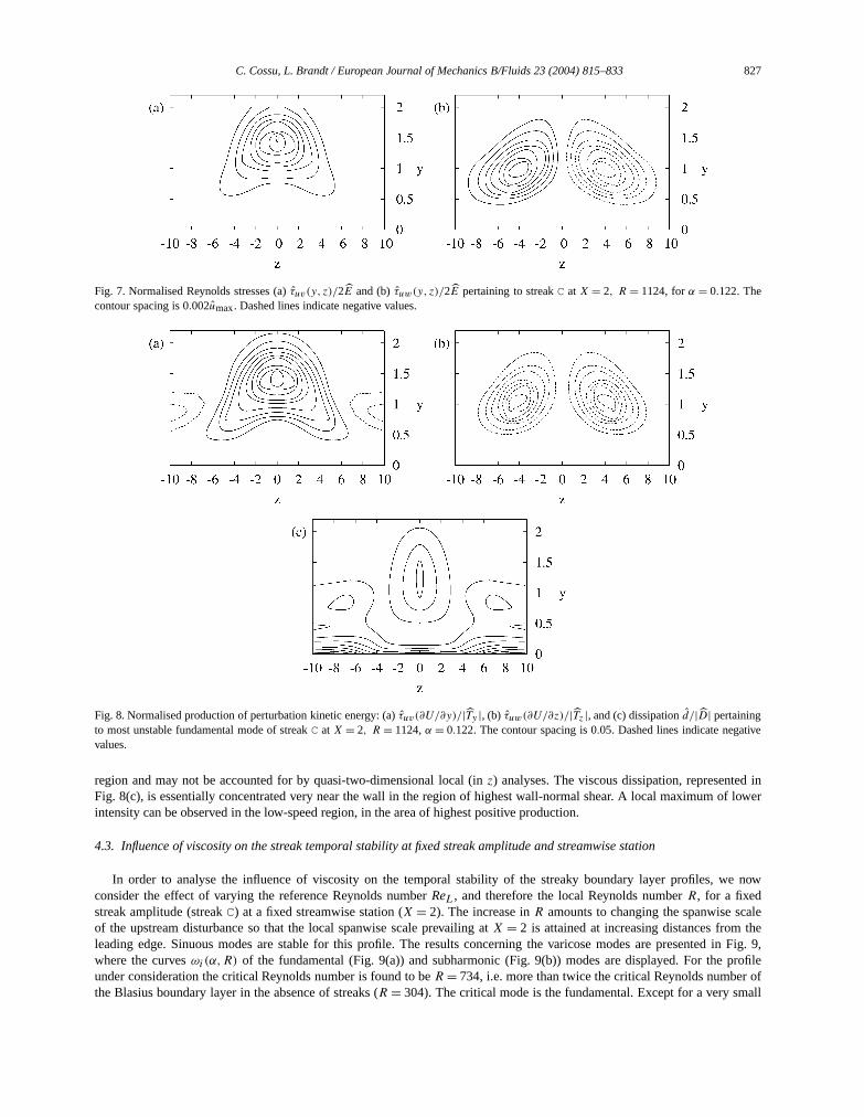
Fig. 7. Normalised Reynolds stresses (a)τuv(y, z)/2E and (b)τuw(y, z)/2E pertaining to streakC at X = 2, R = 1124, forα = 0.122. Thecontour spacing is 0.002umax. Dashed lines indicate negative values.

Fig. 8. Normalised production of perturbation kinetic energy: (a)τuv(∂U/∂y)/|Ty |, (b) τuw(∂U/∂z)/|Tz |, and (c) dissipationd/|D| pertainingto most unstable fundamental mode of streakC at X = 2, R = 1124,α = 0.122. The contour spacing is 0.05. Dashed lines indicate negativvalues.

region and may not be accounted for by quasi-two-dimensional local (inz) analyses. The viscous dissipation, representeFig. 8(c), is essentially concentrated very near the wall in the region of highest wall-normal shear. A local maximum ointensity can be observed in the low-speed region, in the area of highest positive production.

4.3. Influence of viscosity on the streak temporal stability at fixed streakamplitude and streamwise station

In order to analyse the influence of viscosity on the temporal stability of the streakyboundary layer profiles, we nowconsider the effect of varying the reference Reynolds numberReL, and therefore the local Reynolds numberR, for a fixedstreak amplitude (streakC) at a fixed streamwise station (X = 2). The increase inR amounts to changing the spanwise scof the upstream disturbance so that the local spanwise scale prevailing atX = 2 is attained at increasing distances fromleading edge. Sinuous modes are stable for this profile. The results concerning the varicose modes are presentedwhere the curvesωi(α,R) of the fundamental (Fig. 9(a)) and subharmonic (Fig. 9(b)) modes are displayed. For theunder consideration the critical Reynolds number is found to beR = 734, i.e. more than twice the critical Reynolds numbethe Blasius boundary layer in the absence of streaks (R = 304). The critical mode is the fundamental. Except for a very sm


r

wised

largerte valuesbehaviour

erneutral,

. 10 is thesudeic

lds

ity

e

e

the effect

nd

Fig. 9. Growth rateωi of the varicose fundamental (a) and subharmonic (b) modes in the streamwise wavenumberα and local Reynolds numbeR plane for theC streak profile atX = 2. Contours start from the neutral curve and proceed, outer to inner, with a spacing of 10−4.

Fig. 10. Neutral stability curves of (a) the fundamental varicoseand (b) subharmonic varicose modes as a function of the streamwavenumberα and the local Reynolds numberR for the Blasius profile (caseA) and streaksB, C, andD (outermost to inner curves) extracteat X = 2. Subharmonic modes of streakB profiles are stable in the considered Reynolds number range.

region in the parameter plane (roughlyα < 0.07 andR > 1100), the subharmonic varicose modes become unstable atReynolds numbers and their growth rates are smaller than those of the fundamental modes. In principle, intermediaof the detuning parameter should also be examined. However, previous results (see, e.g., [25,26]) show a monotonicwith the Floquet exponent so that the fundamental and subharmonic modes can be seen as the limiting cases.

To compare the combined effects of viscosity and streak amplitude at fixedX, we repeated the calculations for the othstreak profiles atX = 2. In Figs. 10(a) and 10(b) we display, respectively, the varicose fundamental and subharmoniccurves pertaining to each streak. The effect of increasing streak amplitude is todelay the instability ofthe fundamental modesas expected from the results in the previous section (see Fig. 4). The outermost neutral curve shown on the left of Figwell-known neutral curve of the Blasius boundary layer (caseA, with a critical Reynolds numberR = 304). The neutral curvecorresponding to streaks of increasing amplitudeB, C andD are regularly ordered from outer to inner. The largest amplitprofile, the one corresponding to streakD, is able to delay the instability up toR ≈ 1270. The amplitude effect on subharmonmodes, as also seen in the previous section, is not monotone; theC andD profiles exhibit essentially the same critical Reynonumber,R ≈ 1100.

It is important to note that the neutral curves presented in Fig. 10 arelocal neutral curves corresponding to the veloc

profiles prevailing atX = 2. The variation ofR = Re1/2X

= (XReL)1/2 has been obtained through a variation ofReL at fixedX,i.e. through a variation of the spanwise scale at the inlet, byexploiting the scaling property introduced in Section 2.

4.4. Stability along the streaky boundary layer

We now consider the stability of a streakyboundary layer by examining the properties of its profiles at different streamwisstationsX. For the selectedX we choose a range of local Reynolds numberR and compute the growth ratesωi(α;R,X).The maximum growth rateωi,max(R,X) is obtained by maximisingωi overα for eachR andX. The results pertaining to thvaricose modes of streakD, which is the one of largest allowed amplitude before the onset of sinuous inflectional instabilities,are documented in Fig. 11. From the previous sections we know that, for the Reynolds numbers under consideration,of increasingR is destabilising. This is confirmed by the analysis of Fig. 11, where it is seen that, for a constantX, an increasein R leads to instability and then to an increase of the maximum growth rate in the unstable region for both fundamental a


ent

ffect ons,t.

sesose of the

nd free-ce

at

m

dmof

y, for

isplayed in

d

eakhat if thee

Fig. 11. Maximum growth rateωi,max of (a) varicose fundamental and (b) subharmonic modes pertaining to streakD as a function of streamwisstationX and local Reynolds numberR. Contour levels are 0 (thick line), 2× 10−4, 4 × 10−4, 6 × 10−4, . . . . The dashed lines represephysically realizable streaks atReL = 2× 105,4× 105, . . . ,106.

subharmonic modes. The coordinateX describes the downstream evolution of the streaks and, as a consequence, its ethe variation of the flow stability featuresis closely related to the local streak amplitude. Concerning the fundamental modewe have shown that an increasing streak amplitude is stabilising. The maximum amplitude of streakD is attained roughly aX = 2 whenT or As are used as measures of the streak amplitude and roughly atX = 2.5, whenEU is used (see Fig. 1)The former measure seems to better account for the effects of the streak amplitude on the boundary layer stability; in fact,upstream of the peak amplitude (X < 2.5), we observe that increasingX at constantR is stabilising since asX increases thestreak amplitude also increases. Downstream of the peak amplitude (X > 2.5), whenX increases the streak amplitude decreatherefore leading to an increase of the growth rates. Subharmonic modes exhibit growth rates generally lower than thfundamental modes.

A streaky boundary layer obtained in an experiment or in a numerical simulation sees the same viscosity astream velocity at each streamwise station�X. Physically realizable streaks are therefore obtained at fixed referenReynolds numberReL. Along a ‘physical streak’ the local Reynolds number is given byR = (ReLX)1/2, whereReL isa constant. To visualise the stability properties of physically realizable streaks, dashed lines corresponding to streaksReL = 200000,400000, . . . ,1000000 are introduced on Fig. 11. AsX increases, the local Reynolds numberR also increasesso that the effects of varyingX andR on the stability are coupled. In particular, in the part of the streak which is upstreaof its maximum amplitude, the destabilising role of increasingR and the stabilising role of increasingX are in competition.Assuming, for instance,ReL = 200000, streakD is stable up toX = 3.95, corresponding toR ≈ 880, to both varicose ansubharmonic modes. ForReL = 500000 a pocket of instability to both varicose and subharmonic modes appears in the upstreapart of the streak (roughlyX < 1.5) where the streak amplitude is not large enoughto counterbalance the destabilising effectthe Reynolds numberR. In the range 1.5 < X < 2.7 the stabilising effect of the streak amplitude dominates, but eventuallX > 2.7, at roughlyR = 1160, fundamental modes become unstable again.

The computations have been repeated for the others streaky basic flows; the corresponding neutral curves are dFig. 12. As expected, streakD is the most effective in delaying the instability. Thefundamental-mode neutral curve for thelowest amplitude streak is very close to the neutral curve of the Blasius boundary layer, which becomes unstable atR = 304 forall X. It can be seen that for all the streaks under consideration the maximum amplitude profile, prevailing atX ≈ 2.5, may bestable for quite large values ofR (e.g.R = 1270 for streakD). However, the stability of a physically realizable streak, obtainefollowing one of the dashed lines in the plot, may be obtained only up to lowerR values (e.g.R = 880 for streakD) because inthe upstream part of the streak the amplitude is not large enough to counterbalance the destabilising increase ofR. This effectis particularly strong for the streaks we consider here because, as their growth is optimised, they have, upstream of their pvalue, amplitudes that are generally lower than for other possible non-optimal streaks. It should in fact be observed tupstream vortices are induced using wall-roughness elements or blowing-suction slots, their amplitude evolution would not bthe same as for the optimal perturbations used here (see, e.g., [20]).


led heatingdelayingr can bem the basict

gion of

be

rere, and,a strongerrythe highatte

e Fig. 4),It can be

nge Blasius

ation of theenerate thed by active

sd,nalhroughlay the

Fig. 12. Neutral stability curves for (a) fundamental varicoseand (b) subharmonic varicose modes for the Blasius boundary layerA and thestreaksB, C andD as a function of streamwise stationX and local Reynolds numberR. The dashed lines represent physically realizable streaksat ReL = 2× 105,4× 105, . . . ,106.

4.5. Implications for transition delay

Most of ‘open-loop’ transition delay methods rely on the suppression or reduction of the exponential growth of the unstabwaves in the linear regime, obtained for instance by enforcing favourable pressure gradients, through wall suction, fluior cooling, etc. The forcing of steady streaks in a flat plate boundary layer might be as effective as other methods intransition. A clear advantage of this scheme is the fact that the ‘actuators’ modifying the basic flow stability behaviouplaced upstream of the unstable region and presumably require little energy because the streak extracts its energy froflow itself through the ‘lift-up’ effect. In the previous section we have shown that for streakD it is possible to delay the onseof instability up toR above 850 (corresponding toRδ∗ above 1450 andReX above 720000) by choosingReL = 200000. ForlargestReL a pocket of instability appears in the upstream part of the streak, which is however followed by a large restable flow.

To allow a quantitative comparison with other transition delay methods, the computation of spatial growth rates wouldnecessary to estimate the total growths at fixed real frequency (the so calledn-factors used in the eN method). Further, acomplete analysis of the possible transition delay would also require a parametric study of the spanwise wavenumbeβ of thestreaks. The wavelength of optimal spatial growth is not necessarily optimal for the stabilisation process investigated hin fact, one may expect that streaks of larger wave numbers, thus associated with stronger spanwise gradients, havestabilising effect. Such a parametric studyis not attempted in this article since thecomputation of a number of streaky boundalayers with different spanwise wave numbers and amplitudes is still a formidable task. The aim of the paper is to showpotentiality of spanwise modulated flows todelay viscous instabilities and give a physical explanation for it. We believe than experimental study is now more adequate to explore the effect of the wavenumberβ and estimate the spatial growth rareductions.

However, by considering the temporal growth rates and computing the group velocities from the results obtained (seit is possible, using Gaster’s transformation, to roughly estimate the spatial growth rates from the temporal results [55].shown that large reductions of the growth rates are attained both in the pocket of instability observed at lowX and downstreamof the neutral curves. For the fundamental varicose instability, the estimated growth rates are less than half of those pertainito the two-dimensional boundary layer, while the growth rates of the subharmonic modes are about 1% of those of thprofile.

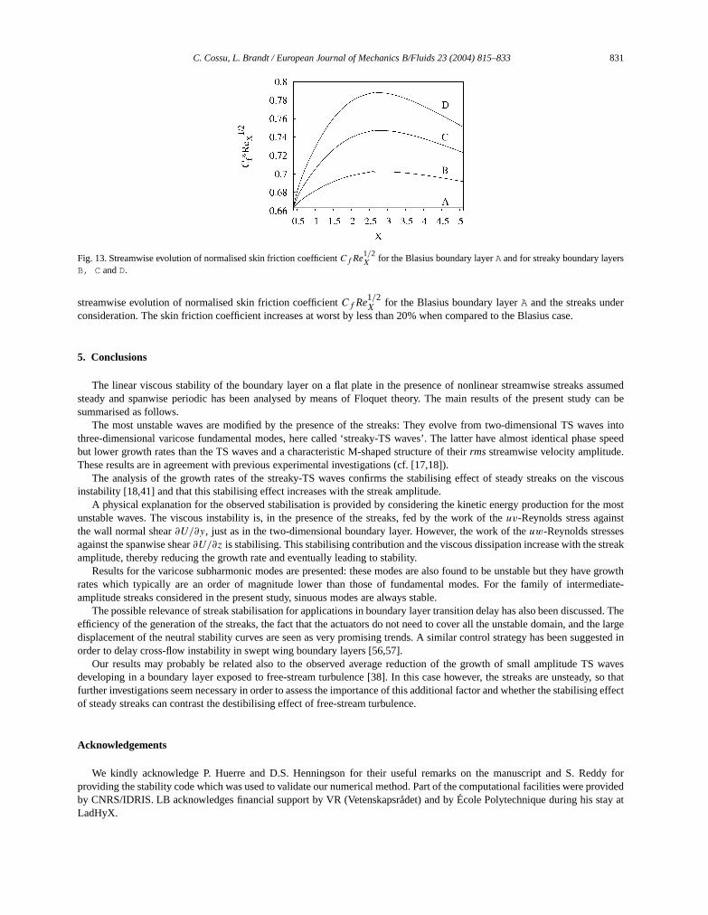
To evaluate the performance of the proposed control strategy one must also evaluate the energy used in the generstreaks and the energy loss due to the presence of the streaks in the boundary layer. No external energy is needed to gstreaks if passive methods, like vortex generators or roughness elements, are used. If instead the streaks are inducemethods, like blowing and suction at the wall, the energy used canstill be considered negligiblebecause the ‘lift-up’ effect actas an amplifier of the actuator energy. Typically the lift-up gain is of orderReX in the linear approximation. On the other hanthe skin friction coefficientCf pertaining to theB, C andD basic flows is larger than that of the Blasius two-dimensioboundary layer. TheCf increase is due to the spanwise uniform part of the basic flow distortion induced by the streaks tnonlinear effects. These lead to ‘fuller’ velocity profiles (see CB) and to larger shear at the wall. On Fig. 13 we disp


s

r

eddy can be

aves intoase speed.

viscous

oststsstreak

ave growthediate-

. Thed the large

in

S wavesdy, so thatsing effect

ddy for

s stay at

Fig. 13. Streamwise evolution of normalised skin friction coefficientCf Re1/2X for the Blasius boundary layerA and for streaky boundary layer

B, C andD.

streamwise evolution of normalised skin friction coefficientCf Re1/2X

for the Blasius boundary layerA and the streaks undeconsideration. The skin friction coefficient increases at worst by less than 20% when compared to the Blasius case.

5. Conclusions

The linear viscous stability of the boundary layer on a flat plate in the presence of nonlinearstreamwise streaks assumsteady and spanwise periodic has been analysed by means of Floquet theory. The main results of the present stusummarised as follows.

The most unstable waves are modified by the presence of the streaks: They evolve from two-dimensional TS wthree-dimensional varicose fundamental modes, here called ‘streaky-TS waves’. The latter have almost identical phbut lower growth rates than the TS waves and a characteristic M-shaped structure of theirrmsstreamwise velocity amplitudeThese results are in agreement with previous experimental investigations (cf. [17,18]).

The analysis of the growth rates of the streaky-TS waves confirms the stabilising effect of steady streaks on theinstability [18,41] and that this stabilising effect increases with the streak amplitude.

A physical explanation for the observed stabilisation is provided by considering the kinetic energy production for the munstable waves. The viscous instability is, in the presence of the streaks, fed by the work of theuv-Reynolds stress againthe wall normal shear∂U/∂y, just as in the two-dimensional boundary layer. However, the work of theuw-Reynolds stresseagainst the spanwise shear∂U/∂z is stabilising. This stabilising contribution and the viscous dissipation increase with theamplitude, thereby reducing the growth rate and eventually leading to stability.

Results for the varicose subharmonic modes are presented: these modes are also found to be unstable but they hrates which typically are an order of magnitude lower than those of fundamental modes. For the family of intermamplitude streaks considered in the present study, sinuous modes are always stable.

The possible relevance of streak stabilisation for applications in boundary layer transition delay has also been discussedefficiency of the generation of the streaks, the fact that the actuators do not need to cover all the unstable domain, andisplacement of the neutral stability curves are seen as very promising trends. Asimilar control strategy has been suggestedorder to delay cross-flow instabilityin swept wing boundary layers [56,57].

Our results may probably be related also to the observed average reduction of the growth of small amplitude Tdeveloping in a boundary layer exposed to free-stream turbulence [38]. In this case however, the streaks are unsteafurther investigations seem necessary in order to assess the importance of this additional factor and whether the stabiliof steady streaks can contrast the destibilising effect of free-stream turbulence.

Acknowledgements

We kindly acknowledge P. Huerre and D.S. Henningson for their useful remarks on the manuscript and S. Reproviding the stability code which was used to validate our numerical method. Partof the computational facilities were providedby CNRS/IDRIS. LB acknowledges financial support by VR (Vetenskapsrådet) and by École Polytechnique during hiLadHyX.


References

999)

id

181,

ley,

ent

nce,

(1987).wise

1.

.–

001)

, in:. 17–

,

314.ent

nce,

m

s,

77–

ys.

[1] H. Schlichting, Boundary-Layer Theory, McGraw-Hill, New York, 1979.[2] M.T. Landahl, Wave breakdown and turbulence, SIAM J. Appl. Math. 28 (1975) 735–756.[3] T. Ellingsen, E. Palm, Stability of linear flow, Phys. Fluids 18 (1975) 487–488.[4] L.H. Gustavsson, Energy growth of three-dimensional disturbances in plane Poiseuille flow, J. Fluid Mech. 224 (1991) 241–260.[5] S.C. Reddy, D.S. Henningson, Energy growth inviscous channel flows, J. Fluid Mech. 252 (1993) 209–238.[6] P.J. Schmid, D.S. Henningson, Stability and Transition in Shear Flows, Springer, New York, 2001.[7] P. Andersson, M. Berggren, D.S. Henningson, Optimal disturbances and bypass transition in boundary layers, Phys. Fluids 11 (1

134–150.[8] P. Luchini, Reynolds-number independent instability of the boundary layer over a flat surface. Part 2: Optimal perturbations, J. Flu

Mech. 404 (2000) 289–309.[9] M. Choudhari, Boundary-layer receptivity to three-dimensional unstaedy vortical disturbances in the free stream, AIAA Paper 96, 0

1996.[10] F.P. Bertolotti, Response of the Blasius boundary layer to free-stream vorticity, Phys. Fluids 9 (8) (1997) 2286–2299.[11] D.W. Wundrow, M.E. Goldstein, Effect on a laminar boundary layer of small-amplitude streamwise vorticity in the upstream flow, J. Fluid

Mech. 426 (2001) 229–262.[12] H.L. Dryden, Air flow in the boundary layer near a plate. Report 562, NACA, 1937.[13] G.I. Taylor, Some recent developments in the study of turbulence, in: J. Hartog, H. Peters (Eds.), Proc. 5th Int. Congr. Appl. Mech., Wi

1939, pp. 294–310.[14] D. Arnal, J.C. Juillen, Contribution expérimentale à l’étude de la reptivité d’une couche limite laminaire à la turbulence de l’écoulem

général, Rapport Technique 1/5018, ONERA, 1978.[15] J.M. Kendall, Experimental study of disturbances produced in a pre-transitional laminar boundary layer by weak free-stream turbule

AIAA Paper 85 (1985) 1695.[16] P.S. Klebanoff, Effect of free-stream turbulenceon the laminar boundary layer, Bull. Am. Phys. Soc. 10 (1971) 1323.[17] I. Tani, H. Komoda, Boundary layer transition in the presence of streamwise vortices, J. Aerospace Sci. 29 (1962) 440.[18] Y.S. Kachanov, O.I. Tararykin, Experimental investigation of a relaxating boundary layer, Izv. SO AN SSSR Ser. Tech. Nauk 18[19] A.A. Bakchinov, G.R. Grek, B.G.B. Klingmann, V.V. Kozlov, Transition experiments in a boundary layer with embedded stream

vortices, Phys. Fluids 7 (1995) 820–832.[20] E.B. White, Transient growth of stationary disturbances in a flat plate boundary layer, Phys. Fluids 14 (2002) 4429–4439.[21] L. Prandtl, Bemerkungen über die Enstehung der Turbulenz, ZAMM 1 (1921) 431–435.[22] W. Tollmien, Über die Entstehung der Turbulenz, Nachr. Ges. Wiss. Göttingen 21–24 (1929). English translation NACA TM 609, 193[23] H. Schlichting, Berechnung der Anfachung kleiner Störungen bei der Plattenströmung, ZAMM 13 (1933) 171–174.[24] G.B. Schubauer, H.F. Skramstad, Laminar boundary layer oscillations and the stabilityof laminar flow, J. Aero. Sci. 14 (1947) 69–78.[25] T. Herbert, Secondary instability of boundary-layers, Annu. Rev. Fluid Mech. 20 (1988) 487–526.[26] P. Andersson, L. Brandt, A. Bottaro, D.S. Henningson, On the breakdown of boundarylayers streaks, J. Fluid Mech. 428 (2001) 29–60[27] L. Brandt, D.S. Henningson, Transition of streamwise streaks inzero-pressure-gradient boundary layers, J. Fluid Mech. 472 (2002) 229

262.[28] M. Matsubara, P.H. Alfredsson, Disturbance growth in boundary layers subjected to free stream turbulence, J. Fluid. Mech. 430 (2

149–168.[29] R.G. Jacobs, P.A. Durbin, Simulationsof bypass transition, J. Fluid Mech. 428 (2001) 185–212.[30] W. Schoppa, F. Hussain, Coherent structure generation in near-wall turbulence, J. Fluid Mech. 453 (2002) 57–108.[31] L. Brandt, P. Schlatter, D.S. Henningson, Numerical simulationsof transition in a boundary layer under free-stream turbulence

I. Castro, P.E.H. Thomas (Eds.), Advances in Turbulence IX, Proc.of the Ninth European Turbulence Conference, Springer, 2002, pp20.

[32] L. Brandt, Numerical studies of bypass transition in the Blasiusboundary layer. Ph.D. thesis, Royal Institute of Technology, StockholmSweden, 2003.

[33] M. Asai, M. Minagawa, M. Nishioka, The instability and breakdown of a near-wall low-speed streak, J. Fluid Mech. 455 (2002) 289–[34] X. Wu, M. Choudhari, Linear and nonlinear instabilities of a Blasius boundary layer perturbed by streamwise vortices. Part II: Intermitt

instability induced by long-wavelength Klebanoff modes, J. Fluid Mech. 483 (2003) 249–286.[35] H.L. Reed, W.S. Saric, Stability of three-dimensional boundary layers, Annu. Rev. Fluid Mech. 21 (1989) 235–284.[36] H. Komoda, Nonlinear development of disturbancein a laminar boundary layer, Phys. Fluids Suppl. 10 (1967) S87.[37] H.R. Grek, V.V. Koslov, M.P. Ramazanov, Investigation of boundary layer stability in the presence of high degree of free-stream turbule

in: Proc. of Int. Seminar of Problems of Wind Tunnel Modeling, vol. 1, Novosibirsk, 1989 (in Russian).[38] A.V. Boiko, K.J.A. Westin, B.G.B. Klingmann, V.V. Kozlov, P.H. Alfredsson, Experiments in aboundary layer subjected to free strea

turbulence. Part 2. The role of TS-waves in the transition process, J. Fluid Mech. 281 (1994) 219–245.[39] X. Wu, J. Luo, Linear and nonlinear instabilities of a Blasius boundarylayer perturbed by streamwise vortices. Part 1. Steady streak

J. Fluid Mech. 483 (2003) 225–248.[40] M.E. Goldstein, D.W. Wundrow, Interaction of oblique instability waves with weak streamwise vortices, J. Fluid Mech. 284 (1995) 3

407.[41] C. Cossu, L. Brandt, Stabilization of Tollmien–Schlichting waves by finite amplitude optimalstreaks in the Blasius boundary layer, Ph

Fluids 14 (2002) L57–L60.


[42] M.N. Kogan, M.V. Ustinov, Boundary layer stabilization by “artificial turbulence”, Fluid Dynamics 38 (2003) 571–580.[43] P. Hall, N.J. Horseman, The linear inviscid secondary instability oflongitudinal vortex structures in boundary-layers, J. Fluid Mech. 232

rtler

343.el

f

ry

ted

283

it, Fluid

id

yer,

(1991) 357–375.[44] X. Yu, J. Liu, On the secondary instability in Goertler flow, Phys. Fluids A 3 (1991) 1845.[45] X. Yu, J. Liu, On the mechanism of sinuous and varicose modes in three-dimensional viscous secondary instability of nonlinear Gö

rolls, Phys. Fluids 6 (2) (1994) 736–750.[46] F. Waleffe, Hydrodynamic stability and turbulence: beyond transients to a self-sustaining process, Stud. Appl. Math. 95 (1995) 319–[47] S.C. Reddy, P.J. Schmid, J.S. Baggett, D.S. Henningson, On the stability of streamwise streaks and transition thresholds in plane chann

flows, J. Fluid Mech. 365 (1998) 269–303.[48] A. Lundbladh, S. Berlin, M. Skote, C. Hildings, J. Choi, J. Kim, D.S. Henningson, An efficient spectral method for simulation o

incompressible flow over a flat plate, Technical Report KTH/MEK/TR-99/11-SE, KTH, Department of Mechanics, Stockholm, 1999.[49] L. Brandt, C. Cossu, J.-M. Chomaz, P. Huerre, D.S. Henningson, On the convectivelyunstable nature of optimal streaks in bounda

layers, J. Fluid Mech. 485 (2003) 221–242.[50] P. Drazin, W. Reid, Hydrodynamic Stability, Cambridge Univ. Press, 1981.[51] C. Canuto, Y.M. Hussaini, A. Quarteroni, T.A. Zang,Spectral Methods in Fluid Dynamics, Springer, New York, 1988.[52] R.B. Lehoucq, D.C. Sorensen, C. Yang, ARPACK user guide: Solution of Large-Scale Eigenvalue Problems with Implicitly Restar

Arnoldi Methods, SIAM, Philadelphia, 1998.[53] D.S. Park, P. Huerre, Primary and secondary instabilities of the asymptotic suction boundary layer on a curved plate, J. Fluid Mech.

(1995) 249–272.[54] M.V. Ustinov, Stability of the flow in a streaky structure and the development of perturbations generated by a point source inside

Dynamics 37 (2002) 9–20.[55] M. Gaster, A note on the relation between temporally-increasing and spatially-increasing disturbances in hydrodynamic stability, J. Flu

Mech. 14 (14) (1962) 222–224.[56] W.S. Saric, R.B. Carrillo Jr., M.S. Reibert, Leading-edge roughness as a transition control mechanism, AIAA Paper-98-0781, 1998.[57] P. Wassermann, M. Kloker, Mechanisms and passive control of crossflow-vortex-induced transition in a three-dimensional boundary la

J. Fluid Mech. 456 (2002) 49–84.

on tollmien–schlichting-like waves in streaky …luca/papers/cossu_ejmb.pdfeuropean journal of...

Documents