On Time Inconsistency: A Technical Issue in

Stackelberg Differential Games

(Journal of Economic Theory 1997)

Danyang Xie∗

Department of Economics

Hong Kong University of Science and Technology

Clear Water Bay, Kowloon

Hong Kong

∗I thank William Brock, Gregory Chow, Bentley MacLeod, Torsten Persson, Paul

Romer and Henry Wan, Jr. for helpful discussions. I am grateful to a referee whose

suggestion has strengthened the paper considerably. This research is supported by DAG

at HKUST.

1

Running Head: On Time Inconsistency

Mailing Address:

Professor Danyang XIE

Department of Economics

HKUST

Clear Water Bay, Kowloon

Hong Kong

2

Abstract

Stackelberg differential games are useful settings in which optimal gov-

ernment policies can be studied. This paper argues that the analysis of these

games involves a key technical issue. In particular, we question the necessity

for optimality of one boundary condition invoked in existing literature. The

issue is of key interest because the boundary condition is largely responsible

for the time inconsistency results previously obtained. We show that the

boundary condition is not necessary in some cases. As a result, our finding

undermines the credibility of the existing conclusions. Journal of Economic

Literature Classification Numbers: C61, E62, H21.

3

1 Introduction

Stackelberg differential games have often been used to study dynamic inter-

action between government and private agents. The government naturally

plays the role of the leader, setting monetary and fiscal policies. Private

agents are the followers, responding optimally to government policy in their

decision on consumption, investment, labor supply and so on. The govern-

ment then takes the private agents’ best response into account and forms the

optimal policy. Examples using such a framework can be found in Kydland

and Prescott [10], Calvo [4], Turnovsky and Brock [15], Lucas and Stokey

[11], Chamley [7], and Persson, Persson and Svensson [13].

The pioneering work by Kydland and Prescott [10] has created the “time

inconsistency” literature, which generally falls into two categories. In the

first category, the studies determine which optimal government policies tend

to be time inconsistent. Calvo [4], Turnovsky and Brock [15] and Chamley

[7] are examples in this category.

In the second category, the studies examine the debt instruments the

incumbent government can use to bind the action of its successor and thus

ensure time consistency. Lucas and Stokey [11] and Persson, Persson and

Svensson [13] are representative.

The work in the second category carries an optimistic tone that the time

inconsistent optimal policy can be made time consistent through intentional

debt management by governments. A technical error found in Persson, Pers-

son and Svensson [13] shatters such a hope (see Calvo and Obstfeld [6]). Re-

cent attempts in characterizing time consistent policies without commitment

include Calvo and Guidotti [5], Benhabib and Rustichini [1] and Benhabib,

4

Rustichini and Velasco [2]. Calvo and Guidotti show that a second-best

incentive compatible outcome can be reached by manipulating government

debt maturity. Benhabib et al. show that incentive compatible outcomes can

be maintained through reputational mechanisms and they conduct numerical

analysis to see how differences in taxes with and without commitment are

affected by parameter changes.

The work in the first category also suffers from technical inadequacy as

this paper will argue. Unless the issue raised here is resolved, the results

obtained in a number of existing papers remain questionable.

To put it simply, the technical inadequacy lies in a failure to prove that the

boundary conditions imposed in various papers are necessary for optimality.

In particular, we show that one of the boundary conditions is not necessary

in some cases. Since this boundary condition is responsible for deriving time

inconsistency, our finding calls for caution.

This paper only points out a problem but does not offer a solution. We

hope that this paper serves the same purpose as the counter-example in Shell

[14]: The Shell example questions the necessity of a transversality condition

for optimality in infinite horizon and has served as a challenge which leads

to the full resolution of the problem by Weitzman [16] in discrete time and

Benveniste and Scheinkman [3] in continuous time.

The rest of the paper is organized as follows. Section 2 presents a dy-

namic taxation model as a Stackelberg differential game. Section 3 uses the

boundary conditions that are usually imposed in the literature and obtain

the time inconsistency result. Section 4 uses a special parametric example of

the model which permits explicit solution to show that one of the boundary

condition imposed in Section 3 is not necessary for optimality. Thus the

conclusion of time inconsistency reached in Section 3 is spurious. Section 5

discusses the generality of our finding. Section 6 contains an example which

5

shows that the technical issue can arise in the original Chamley framework.

Section 7 concludes.

2 A Model of Dynamic Taxation

We consider an economy populated with a continuum of identical private

agents. These agents are consumers-cum-producers and can be represented

by a set α : α ∈ [0, 1]. They produce a single good which is either

consumed or invested as capital for later production. Production function

for an individual is given by y = f(k) where k is capital and y is output.

Government imposes only an output tax, the entire path of which, τ (t) ∈[0, 1]: t ≥ 0, is announced at time zero. Government spending is in the formof public goods. We require that the government budget be balanced each

period. In other words,

g(t) =Z 1

0f(kα(t))τ(t) dα, for all t ≥ 0, (1)

where g is the amount of public good, kα is the capital stock of individual α.

For an individual α, his optimal consumption and investment plan is the

solution to the following lifetime utility maximization problem:

(Problem α)

maxZ ∞0[U(cα) + V (g)] e

−ρt dt, (2)

subject to kα = f(kα)(1− τ)− cα, with kα0 given, (3)

where cα is individual α’s consumption; the utility functions, U(·) and V (·),and the production function, f(·), are concave and strictly increasing. Fur-thermore, U 0(0) = V 0(0) = +∞.

6

We can characterize the response of individual α to government tax policy

by a set of first order conditions and a transversality condition. To do this,

we use the Hamiltonian:

Hα = [U(cα) + V (g)] + qα [f(kα)(1− τ )− cα] . (4)

Note that g depends on the action of the entire population (see Eq. (1))

and is thus considered as given by any individual. Therefore, the first order

conditions are:

U 0(cα) = qα (5)

qα = ρqα − qαf 0(kα)(1− τ). (6)

The transversality condition is kαqαe−ρt → 0 as t→∞.

For each path τ (t) ∈ [0, 1]: t ≥ 0 that the government announces,there is a corresponding optimal plan of resource allocation over time by each

individual. Since all individuals are assumed to be identical, the subscript α

can be removed from the equations above and the optimal response of private

agents can thus be rewritten as follows:

U 0(c) = q (7)

k = f(k)(1− τ)− c (8)

q = ρq − qf 0(k)(1− τ ) (9)

k0 given and limt→∞ kqe

−ρt = 0. (10)

In equilibrium, Eq. (1) reduces to

g = f(k)τ. (11)

Assume the government shares the same objective function with the repre-

sentative individual. If we invert Eq. (7) to obtain c = c(q), we can write

down the government’s optimization problem as follows:

7

(Problem G)

maxZ ∞0[U(c(q)) + V (f(k)τ )] e−ρt dt,

subject to: k = f(k)(1− τ )− c(q) (12)

q = ρq − qf 0(k)(1− τ ) (13)

k0 given and limt→∞ kqe

−ρt = 0 (14)

This maximization problem has some peculiar aspects. First, the objective

function may not be concave in q. Second, the boundary conditions include

a transversality condition at infinity. As a result, there are no ready-made

necessary boundary conditions we can apply for (Problem G).

The first order conditions should still be straightforward to derive. Let λ

and ξ be the co-state variables for k and q, respectively. We have:

V 0(f(k)τ)f(k) = λf(k)− ξqf 0(k) (15)

λ = ρλ− V 0(f(k)τ )f 0(k)τ − λf 0(k)(1− τ ) + ξqf 00(k)(1− τ) (16)

ξ = ρξ − qc0(q) + λc0(q)− ξ(ρ− f 0(k)(1− τ)) (17)

In the next section, we will see how the boundary conditions convention-

ally imposed imply time inconsistency of optimal government tax policy.

3 Necessary Boundary Conditions

As mentioned in the last section, (Problem G) is not a standard maximization

problem. The necessity of the boundary conditions ought to be established

rigorously. The special aspects of (Problem G) have not received any atten-

tion and researchers simply apply their intuition when selecting the boundary

conditions.

8

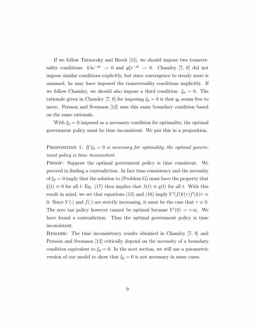
If we follow Turnovsky and Brock [15], we should impose two transver-

sality conditions: kλe−ρt → 0 and qξe−ρt → 0. Chamley [7, 8] did not

impose similar conditions explicitly, but since convergence to steady state is

assumed, he may have imposed the transversality conditions implicitly. If

we follow Chamley, we should also impose a third condition: ξ0 = 0. The

rationale given in Chamley [7, 8] for imposing ξ0 = 0 is that q0 seems free to

move. Persson and Svensson [12] uses this same boundary condition based

on the same rationale.

With ξ0 = 0 imposed as a necessary condition for optimality, the optimal

government policy must be time inconsistent. We put this in a proposition.

Proposition 1: If ξ0 = 0 is necessary for optimality, the optimal govern-

ment policy is time inconsistent.

Proof: Suppose the optimal government policy is time consistent. We

proceed in finding a contradiction. In fact time consistency and the necessity

of ξ0 = 0 imply that the solution to (Problem G) must have the property that

ξ(t) ≡ 0 for all t. Eq. (17) then implies that λ(t) ≡ q(t) for all t. With thisresult in mind, we see that equations (13) and (16) imply V 0(f(k)τ)f 0(k)τ ≡0. Since V (·) and f(·) are strictly increasing, it must be the case that τ ≡ 0.The zero tax policy however cannot be optimal because V 0(0) = +∞. Wehave found a contradiction. Thus the optimal government policy is time

inconsistent.

Remark: The time inconsistency results obtained in Chamley [7, 8] and

Persson and Svensson [12] critically depend on the necessity of a boundary

condition equivalent to ξ0 = 0. In the next section, we will use a parametric

version of our model to show that ξ0 = 0 is not necessary in some cases.

9

4 A Counter Example

In the last section, we showed that the conventional use of the boundary

condition ξ0 = 0 leads to the straightforward conclusion of time inconsistency.

We will show in this section that imposing ξ0 = 0 as a necessary condition

for optimality is spurious.

The parametric class of examples we have is: U(c) = [c1−σ−1]/(1−σ) andf(k) = Akσ where 0 < σ ≤ 1 and A > 01. The simplest case in which σ = 1

is sufficient to demonstrate our argument. In this case, our representative

individual has log utility and linear production:

U(c) = ln(c), V (g) = ln(g), f(k) = Ak.

The private agents’ behavior is now characterized by:

1/c = q (18)

k = Ak(1− τ)− c (19)

q = ρq − qA(1− τ) (20)

k0 given, and kqe−ρt → 0. (21)

Eq. (18) implies that c(q) = 1/q. Substitute this into (19) and multiply

through the equation by q. Add qk to each side, then substitute out q on the

RHS from (20). This leaves

d (qk) /dt = ρqk − 1.1This particular class of utility-production pairs, indexed by σ, can often be used to

obtain closed form solutions in dynamic settings. See Xie [17, 18] for similar examples.

10

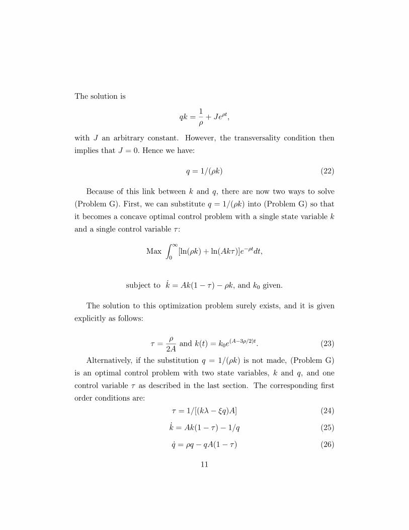
The solution is

qk =1

ρ+ Jeρt,

with J an arbitrary constant. However, the transversality condition then

implies that J = 0. Hence we have:

q = 1/(ρk) (22)

Because of this link between k and q, there are now two ways to solve

(Problem G). First, we can substitute q = 1/(ρk) into (Problem G) so that

it becomes a concave optimal control problem with a single state variable k

and a single control variable τ :

MaxZ ∞0[ln(ρk) + ln(Akτ )]e−ρtdt,

subject to k = Ak(1− τ )− ρk, and k0 given.

The solution to this optimization problem surely exists, and it is given

explicitly as follows:

τ =ρ

2Aand k(t) = k0e

(A−3ρ/2)t. (23)

Alternatively, if the substitution q = 1/(ρk) is not made, (Problem G)

is an optimal control problem with two state variables, k and q, and one

control variable τ as described in the last section. The corresponding first

order conditions are:

τ = 1/[(kλ− ξq)A] (24)

k = Ak(1− τ)− 1/q (25)

q = ρq − qA(1− τ) (26)

11

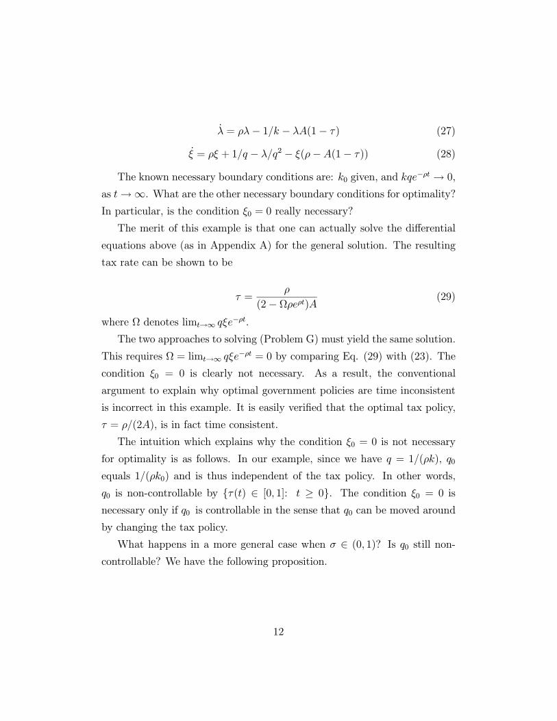
λ = ρλ− 1/k − λA(1− τ) (27)

ξ = ρξ + 1/q − λ/q2 − ξ(ρ−A(1− τ)) (28)

The known necessary boundary conditions are: k0 given, and kqe−ρt → 0,

as t→∞. What are the other necessary boundary conditions for optimality?In particular, is the condition ξ0 = 0 really necessary?

The merit of this example is that one can actually solve the differential

equations above (as in Appendix A) for the general solution. The resulting

tax rate can be shown to be

τ =ρ

(2− Ωρeρt)A(29)

where Ω denotes limt→∞ qξe−ρt.

The two approaches to solving (Problem G) must yield the same solution.

This requires Ω = limt→∞ qξe−ρt = 0 by comparing Eq. (29) with (23). The

condition ξ0 = 0 is clearly not necessary. As a result, the conventional

argument to explain why optimal government policies are time inconsistent

is incorrect in this example. It is easily verified that the optimal tax policy,

τ = ρ/(2A), is in fact time consistent.

The intuition which explains why the condition ξ0 = 0 is not necessary

for optimality is as follows. In our example, since we have q = 1/(ρk), q0

equals 1/(ρk0) and is thus independent of the tax policy. In other words,

q0 is non-controllable by τ (t) ∈ [0, 1]: t ≥ 0. The condition ξ0 = 0 is

necessary only if q0 is controllable in the sense that q0 can be moved around

by changing the tax policy.

What happens in a more general case when σ ∈ (0, 1)? Is q0 still non-controllable? We have the following proposition.

12

Proposition 2. When 0 < σ < 1, the private agents’ best response to the

government tax policy has the property that q = [σ/(ρk)]σ. Therefore, q0 is

determined by k0 and is non-controllable by government tax policies.

Proof: See Appendix B.

Remark: Proposition 2 indicates that the conclusion in the special case

when σ = 1 carries through to the more general case when σ ∈ (0, 1). Thusfor any σ ∈ (0, 1], q0 is non-controllable. As a result, ξ0 = 0 is not necessaryand the optimal tax policy is time consistent.

Note that when σ ∈ (0, 1), both the utility function and the productionfunction are well behaved and satisfy the usual assumptions. Therefore, it is

difficult to rule the class of counter examples out. With general utility and

production functions, explicit solution is impossible. Thus studies that allow

us to identify a priori whether q0 is controllable can help us understand time

inconsistency.

5 Generality of Our Result

In the last section we showed that q0 = 0 is not necessary for optimality for

a class of utility-production pairs indexed by σ. This is because with these

pairs, q0 is non-controllable. There may be other utility-production pairs

with the same property. Time inconsistency result can only be trusted when

these pairs are excluded. Therefore further studies are needed to identify the

cases for exclusion. The following proposition is a start.

Proposition 3. Let U(·) and f(·) be concave and strictly increasing withf(0) = 0. If

f(k)U 0 [ρf(k)/f 0(k)] ≡ J , a constant, (30)

13

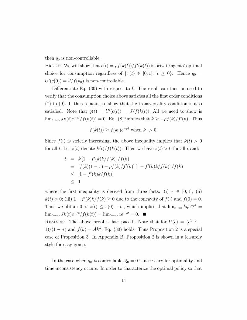
then q0 is non-controllable.

Proof: We will show that c(t) = ρf(k(t))/f 0(k(t)) is private agents’ optimal

choice for consumption regardless of τ(t) ∈ [0, 1]: t ≥ 0. Hence q0 =U 0(c(0)) = J/f(k0) is non-controllable.

Differentiate Eq. (30) with respect to k. The result can then be used to

verify that the consumption choice above satisfies all the first order conditions

(7) to (9). It thus remains to show that the transversality condition is also

satisfied. Note that q(t) = U 0(c(t)) = J/f(k(t)). All we need to show is

limt→∞ Jk(t)e−ρt/f(k(t)) = 0. Eq. (8) implies that k ≥ −ρf(k)/f 0(k). Thus

f(k(t)) ≥ f(k0)e−ρt when k0 > 0.

Since f(·) is strictly increasing, the above inequality implies that k(t) > 0

for all t. Let z(t) denote k(t)/f(k(t)). Then we have z(t) > 0 for all t and:

z = k [1− f 0(k)k/f(k)] /f(k)= [f(k)(1− τ )− ρf(k)/f 0(k)] [1− f 0(k)k/f(k)] /f(k)≤ [1− f 0(k)k/f(k)]≤ 1

where the first inequality is derived from three facts: (i) τ ∈ [0, 1]; (ii)

k(t) > 0; (iii) 1− f 0(k)k/f(k) ≥ 0 due to the concavity of f(·) and f(0) = 0.Thus we obtain 0 < z(t) ≤ z(0) + t , which implies that limt→∞ kqe−ρt =

limt→∞ Jk(t)e−ρt/f(k(t)) = limt→∞ ze−ρt = 0.

Remark: The above proof is fast paced. Note that for U(c) = (c1−σ −1)/(1− σ) and f(k) = Akσ, Eq. (30) holds. Thus Proposition 2 is a special

case of Proposition 3. In Appendix B, Proposition 2 is shown in a leisurely

style for easy grasp.

In the case when q0 is controllable, ξ0 = 0 is necessary for optimality and

time inconsistency occurs. In order to characterize the optimal policy so that

14

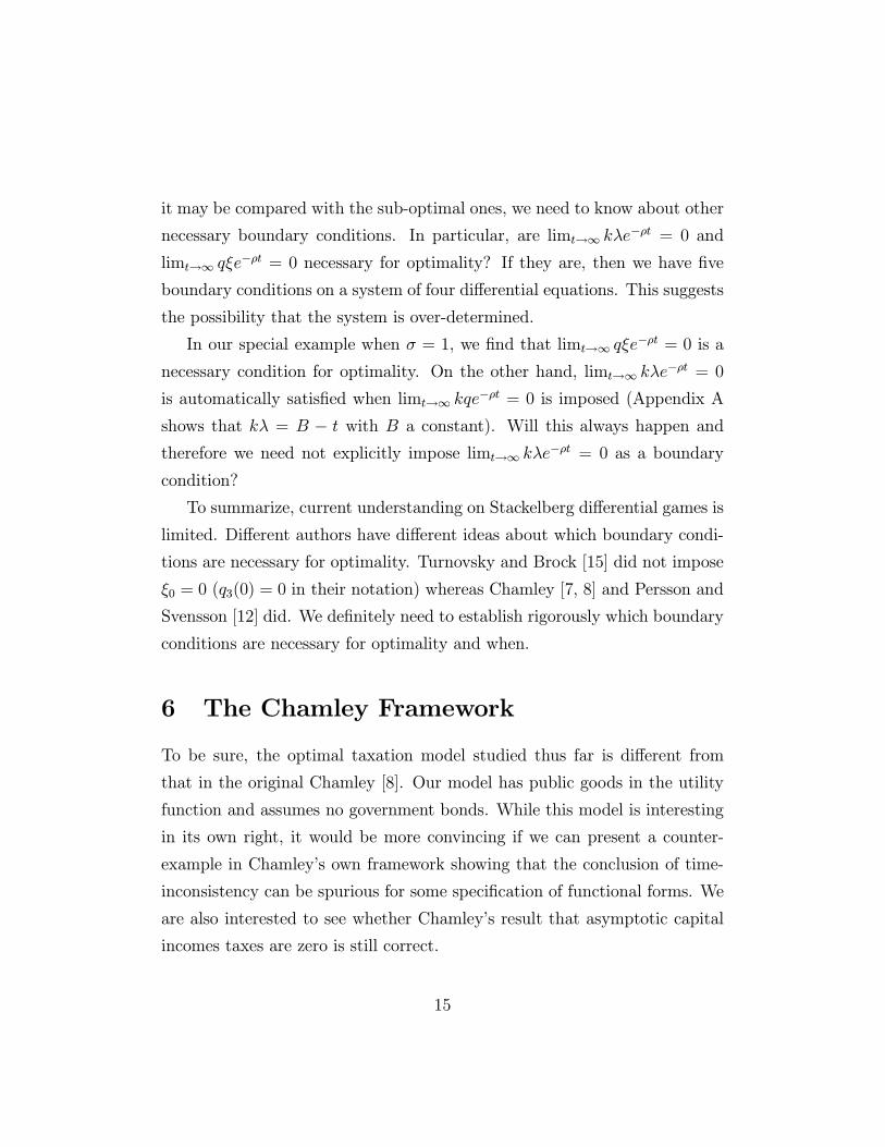
it may be compared with the sub-optimal ones, we need to know about other

necessary boundary conditions. In particular, are limt→∞ kλe−ρt = 0 and

limt→∞ qξe−ρt = 0 necessary for optimality? If they are, then we have five

boundary conditions on a system of four differential equations. This suggests

the possibility that the system is over-determined.

In our special example when σ = 1, we find that limt→∞ qξe−ρt = 0 is a

necessary condition for optimality. On the other hand, limt→∞ kλe−ρt = 0

is automatically satisfied when limt→∞ kqe−ρt = 0 is imposed (Appendix A

shows that kλ = B − t with B a constant). Will this always happen and

therefore we need not explicitly impose limt→∞ kλe−ρt = 0 as a boundary

condition?

To summarize, current understanding on Stackelberg differential games is

limited. Different authors have different ideas about which boundary condi-

tions are necessary for optimality. Turnovsky and Brock [15] did not impose

ξ0 = 0 (q3(0) = 0 in their notation) whereas Chamley [7, 8] and Persson and

Svensson [12] did. We definitely need to establish rigorously which boundary

conditions are necessary for optimality and when.

6 The Chamley Framework

To be sure, the optimal taxation model studied thus far is different from

that in the original Chamley [8]. Our model has public goods in the utility

function and assumes no government bonds. While this model is interesting

in its own right, it would be more convincing if we can present a counter-

example in Chamley’s own framework showing that the conclusion of time-

inconsistency can be spurious for some specification of functional forms. We

are also interested to see whether Chamley’s result that asymptotic capital

incomes taxes are zero is still correct.

15

We assume that the representative agent has the following preferences2:Z ∞0e−ρt ln [c− l] dt (31)

where c is consumption and l is the effort put into work.

The representative firm has a Cobb-Douglas production function,

y = Akαl1−α (32)

where k is the capital stock.

Given real interest rate r and the real wage w, the firm maximizes its

profit by choosing k and l according to the following equations:

r = αAkα−1l1−α (33)

w = (1− α)Akαl−α (34)

As before, we first study the private agent’s utility maximization problem

and then ask what tax policies the government should adopt. Define a as an

individual’s total wealth, a = k + b, where b is the government bonds that

this individual holds. For a given series of τk(t), τl(t)∞0 , the representativeagent maximizes (31) subject to

a = r(1− τk)a+ w(1− τl)l − c (35)

with a0 = k0 + b0 given.

Let q be the co-state variable associated with a. The first order conditions

are:1

c− l = q (36)

2The preferences structure is borrowed from Greenwood, Hercowitz, and Huffman [9].

They use u(c, l) =hc− l1+θ

1+θ

i1−γ/(1 − γ). We simply take the special case: γ = 1 and

θ = 0.

16

1

c− l = qw(1− τl) (37)

q = ρq − qr(1− τk) (38)

The initial condition and the transversality condition is

a0 given and aqe−ρt → 0 (39)

Equations (36) and (37) imply:

w(1− τl) = 1 (40)

and

c = l +1

q(41)

Substituting (40) and (41) into the wealth accumulation equation, we obtain,

a = r(1− τk)a− 1q

This equation, combined with (38), yields,

1

aq

d(aq)

dt= ρ− 1

aq

With the transversality condition (39) imposed, this differential equation has

a unique solution,

aq =1

ρ(42)

This tight relationship between a and q once again demonstrates that con-

trollability problem can also arise in the original Chamley framework. If

we followed what Chamley does, namely imposing ξ0 = 0 (ξ is the co-state

variable on q) as a necessary condition in the government problem, we would

immediately obtain time-inconsistency. This conclusion of time-inconsistency

is however spurious because now we know that whenever controllability prob-

lem arises, ξ0 = 0 is not necessary.

17

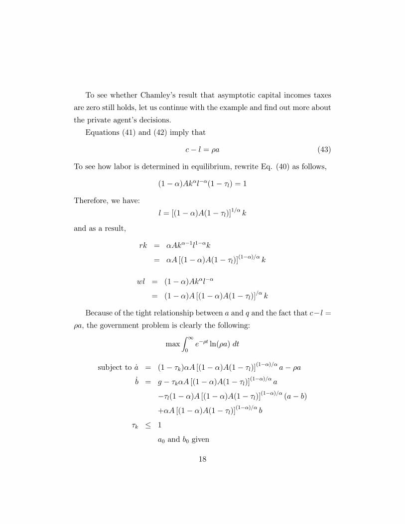
To see whether Chamley’s result that asymptotic capital incomes taxes

are zero still holds, let us continue with the example and find out more about

the private agent’s decisions.

Equations (41) and (42) imply that

c− l = ρa (43)

To see how labor is determined in equilibrium, rewrite Eq. (40) as follows,

(1− α)Akαl−α(1− τl) = 1

Therefore, we have:

l = [(1− α)A(1− τl)]1/α k

and as a result,

rk = αAkα−1l1−αk

= αA [(1− α)A(1− τl)](1−α)/α k

wl = (1− α)Akαl−α

= (1− α)A [(1− α)A(1− τl)]/α k

Because of the tight relationship between a and q and the fact that c−l =ρa, the government problem is clearly the following:

maxZ ∞0e−ρt ln(ρa) dt

subject to a = (1− τk)αA [(1− α)A(1− τl)](1−α)/α a− ρa

b = g − τkαA [(1− α)A(1− τl)](1−α)/α a

−τl(1− α)A [(1− α)A(1− τl)](1−α)/α (a− b)

+αA [(1− α)A(1− τl)](1−α)/α b

τk ≤ 1

a0 and b0 given

18

Where g is the exogenous government spending and is assumed to be

constant for simplicity3. We show in Appendix C that the optimal taxation

policy is:

τk =

1 when t < T

0 when t ≥ Tτl = 0 for all t

where T is determined in the following equation:

ra0ρ+ r

h1− e−(ρ+r)T

i= b0 +

g

r(44)

where r is the pre-tax real interest rate αA [(1− α)A](1−α)/α.

In order for the solution T to be finite, we need

ra0ρ+ r

> b0 +g

r

Eq. (44) is intuitive. It says that the higher the government spending,

the longer the regime of 100% capital income taxation will have to last. Also,

the more debt the government inherits at time zero, the longer the regime of

100% capital income taxation will have to last.

To summarize, Chamley’s result that τk is asymptotically zero still holds

in our special example. But his claim that after time T , the government

spending is financed by labor income tax seems wrong4. This claim also

provides the intuition for his time inconsistency result stated in his concluding

paragraph that a government may be tempted to raise revenues by future

3If g grows at a rate lower than the real interest rate, similar analysis can be done. We

need to find a T so that b(T ) is sufficiently negative and b grows at the same rate as the

government spending for t ≥ T .4Chamley [8] does not have any discription of the optimal wage tax but does claim that

the government spending after time T is financed only by taxing wage income (page 617).

19

levies on capital. Our special example illustrates that in some cases q0 is non-

controllable and thus ξ0 = 0 is not a necessary condition for optimality in the

government problem. This destroys the time inconsistency result technically.

Not only that, the example also destroys time inconsistency result intuitively.

After time T , the government owns enough assets (b sufficiently negative)

so that the government spending can be entirely financed by its interest

earnings. The government has no incentive to lengthen the regime of 100%

capital income taxation. The length of this regime, T , is chosen optimally

once and for all.

7 Conclusion

Due to the nature and complexity of Stackelberg differential games, which

boundary conditions are necessary for optimality is an unresolved issue. This

paper shows that the current treatment of the issue is not rigorous and con-

clusion of time inconsistency could be spurious in some cases.

Since the question of the necessity of boundary conditions is directly

related to the time inconsistency result, we must find the answer. This

paper puts the question forward in a series of examples. As in Shell [14],

these examples are very special and are unlikely to be realistic. This does not

mean that we can afford to neglect them. In fact, powerful counter-examples

are always special and unexpected. We hope that our counter-examples will

attract effort for the early resolution of the technical issue in Stackelberg

differential games.

20

Appendix A

Here we derive the general solution for the set of differential equations

(25) to (28) with the known necessary boundary conditions: k0 given and

limt→∞ kqe−ρt = 0

As shown in the main text, equations (25), (26) and the transversal-

ity condition limt→∞ kqe−ρt = 0 imply that q = 1/(ρk). Substitute q =

1/(ρk) into (25). Equations (25) and (27) can then be re-arranged to obtain

d(kλ)/dt = −1. Thus kλ = B − t,where B is any constant. Hence, we can

substitute λ = (B− t)/k = (B−t)ρq into (28) and solve (26) and (28) for ξq.The result is ξq = Ωeρt−2/ρ+(B− t), where Ω = limt→∞ ξqe−ρt. Therefore,

we have

τ =1

(kλ− ξq)A=

ρ

(2− Ωρeρt)A,

which gives the general solution depending on the choice of the value for Ω.

21

Appendix B

In this appendix, we prove Proposition 2 using three lemmas.

When σ ∈ (0, 1), the first order conditions characterizing the private

agents’ behavior are as follows:

c−σ = q (45)

k = Akσ(1− τ )− c (46)

q = ρq − σqAkσ−1(1− τ) (47)

Since the private agents’ maximization problem is a standard one, the

necessary boundary conditions are well established and they are: k0 given

and limt→∞ kqe−ρt = 0.

Lemma 1: The general solution to equations (45) to (47) has the property

that q1/σk = σ/ρ+ Jeρt/σ, with J any constant.

Proof: Let x = q1/σk. Then we have:

x/x = (1/σ)q/q + k/k

= ρ/σ − 1/x

Thus, x = ρx/σ − 1. This differential equation has the general solution:x = σ/ρ+ Jeρt/σ, with J any constant.

Remark: The private agents’ maximization problem is a standard concave

optimal control problem and therefore has a unique solution. Thus in order

to show q = [σ/(ρk)]σ, it remains to show that the transversality condition

limt→∞ kqe−ρt = 0 is satisfied when J = 0.

22

Lemma 2: When J = 0, k ≥ 0 and is bounded from above.

Proof: When J = 0, q1/σk = σ/ρ. Thus, c = ρk/σ. Eq. (46) implies that

−ρk/σ ≤ k ≤ Akσ − ρk/σ.

Since σ < 1, we know that k ≥ 0 and is bounded from above.

Lemma 3: When J = 0, limt→∞ kqe−ρt = 0.

Proof: When J = 0, q1/σk = σ/ρ. We have:

limt→∞ kqe−ρt = limt→∞ k1−σ³q1/σk

´σe−ρt

= limt→∞(σ/ρ)σk1−σe−ρt

= 0. (Lemma 2)

23

Appendix C

In this appendix, we solve the government problem of optimal taxation

policy in our special example under Chamley framework.

maxZ ∞0e−ρt ln(ρa) dt

subject to a = (1− τk)αA [(1− α)A(1− τl)](1−α)/α a− ρa

b = g − τkαA [(1− α)A(1− τl)](1−α)/α a

−τl(1− α)A [(1− α)A(1− τl)](1−α)/α (a− b)

+αA [(1− α)A(1− τl)](1−α)/α b

τk ≤ 1

a0 and b0 given

Let λ and µ be the co-state variables on a and b respectively. Let ν be

the Lagrangian multiplier on τk ≤ 1. The first order conditions are

−(λ+ µ)αA [(1− α)A(1− τl)](1−α)/α a+ ν = 0 (48)

−λ(1− τk)αA [(1− α)A(1− τl)](1−α)/α a

1− α

α(1− τl)

+µτkαA [(1− α)A(1− τl)](1−α)/α a

1− α

α(1− τl)

−µ(1− α)A [(1− α)A(1− τl)](1−α)/α (a− b)

+µτl(1− α)A [(1− α)A(1− τl)](1−α)/α (a− b) 1− α

α(1− τl)

−µαA [(1− α)A(1− τl)](1−α)/α b

1− α

α(1− τl)= 0 (49)

ν(1− τk) = 0 (50)

24

λ = ρλ− 1a− λ

h(1− τk)αA [(1− α)A(1− τl)]

(1−α)/α − ρi

+µhτkαA [(1− α)A(1− τl)]

(1−α)/α + τl(1− α)A [(1− α)A(1− τl)](1−α)/αi

µ = ρµ−µτl(1−α)A [(1− α)A(1− τl)](1−α)/α−µαA [(1− α)A(1− τl)]

(1−α)/α

The initial boundary conditions and the transversality conditions are

a0 and b0 given

aλe−ρt → 0 and bµe−ρt → 0

From the government’s objective function, we see that it is not optimal

to have a = 0 at any moment. Thus a 6= 0 is always true.Also, the constraint τk ≤ 1 can not be binding forever. Let T be the

time after which the constraint is not binding (T = 0 is not ruled out at this

moment).

Consider what happens when t ≥ T . By definition of T , we know thatν(t) = 0. Hence from Eq. (48) and the fact that a 6= 0, we have

λ+ µ = 0

And from (49) and the fact that k = a− b > 0, we have

τl ≡ 0

Combining the differential equations on λ and µ and using the fact that

λ+ µ = 0 , we obtain,

aλ =1

ρ

As a result,

λ = λhρ− αA [(1− α)A](1−α)/α

ia

a+

λ

λ= (1− τk)αA [(1− α)A(1− τl)]

(1−α)/α − ρ+ ρ− αA [(1− α)A](1−α)/α

= −τkαA [(1− α)A](1−α)/α

25

Since aλ = 1/ρ implies that the LHS of the above equation is zero, it

must be true that τk = 0, for t ≥ T . Therefore whenever τk < 1, τk and

τl must be zero. In order for this to be possible, then we must need the

government to own enough private assets at time T so that the returns on

the assets are just sufficient to cover its spending thereafter. In other words,

b = 0 after T . Thus from b equation, we obtain:

b(T ) = − g

αA [(1− α)A](1−α)/α(51)

and b(t) will stay at that level for any t > T .

When t < T , τk = 1 by the definition of T . Eq. (49) can be simplified

and rewritten as follows:

µτl = 0 (52)

Note that −µ has the interpretation of marginal tax excess burden so that µis always negative5. Hence,

τl = 0 (53)

Substitute τk = 1 and τl = 0 to the differential equations on a and b, we find

that for t < T ,

a = −ρab = g − αA [(1− α)A](1−α)/α a+ αA [(1− α)A](1−α)/α b

Note that the constant, αA [(1− α)A](1−α)/α , is the pre-tax real interest rate

r, we can simplify and re-arrange the equation above and then multiply both

5If the government starts with a b0 (negative) which generates interest revenue more

than sufficient to cover its spending, then µ ≡ 0. As in Chamley [8], we assume that it isunlikely for the government to have large negative b at time zero. Therefore µ is strictly

negative. Note that µ(t) remains to be negative even after time T when its interest

revenue is just sufficient to cover its spending. The reason is that any marginal increase

of government spending will activate the use of distortionary taxes and the distortion is

measured by the excess burden −µ.

26

sides by e−rt: hb− rb

ie−rt = ge−rt − ra0e−ρt−rt

Take integral from 0 to T ,

bT e−rT − b0 = g1− e

−rT

r− ra0

ρ+ r

h1− e−(ρ+r)T

iSubstituting in bT = −g/r from Eq. (51), we get an equation that determinesT :

ra0ρ+ r

h1− e−(ρ+r)T

i= b0 +

g

r

Thus, the optimal tax policy is:

τk =

1 when t < T

0 when t ≥ Tτl = 0 for all t

27

References

[1] J. Benhabib, and A. Rustichini, “Optimal Taxes Without Commit-

ment,” Manuscript, December, 1996.

[2] J. Benhabib, A. Rustichini, and A. Velasco, “Public Capital and Optimal

Taxes Without Commitment,” Manuscript, January, 1997.

[3] L. M. Benveniste, and J. A. Scheinkman, Duality Theory for Dynamic

Optimization Models of Economics: The Continuous Time Case, J.

Econ. Theory 27 (1982), 1—19.

[4] G. Calvo, On the Time Consistency of Optimal Policy in a Monetary

Economy, Econometrica 46 (1978), 1411-1428.

[5] G. Calvo and P. Guidotti, Optimal Maturity of Nominal Government

Debt: An Infinite-Horizon Model, Int. Econ. Rev. 33 (1992), 895—919.

[6] G. Calvo and M. Obstfeld, Time Consistency of Fiscal and Monetary

Policy: A Comment, Econometrica 58 (1990), 1245—1247.

[7] C. Chamley, Efficient Taxation in a Stylized Model of Intertemporal

General Equilibrium, Int. Econ. Rev. 26 (1985), 451—468.

[8] C. Chamley, Optimal Taxation of Capital Income in General Equilib-

rium with Infinite Lives, Econometrica 54 (1986), 607—622.

[9] J. Greenwood, Z. Hercowitz, and G. Huffman, Investment, Capacity

Utilization, and the Real Business Cycle, Amer. Econ. Rev. 78 (1988),

402—417.

28

[10] F. Kydland and E. Prescott, Rules Rather than Discretion: The Incon-

sistency of Optimal Plans, J. Polit. Econ. 85 (1977), 473—492.

[11] R. E. Lucas, Jr. and N. Stokey, Optimal Fiscal and Monetary Policy in

an Economy without Capital, J. Monet. Econ. 12 (1983), 55—93.

[12] T. Persson and L. E. O. Svensson, “New Methods in the Swedish

Medium-Term Survey,” Appendix 4, Manuscript, August, 1986.

[13] M. Persson, T. Persson, and L. E. O. Svensson, Time Consistency of

Fiscal and Monetary Policy, Econometrica 55 (1987), 1419—1431.

[14] K. Shell, “Applications of Pontryagin’s Maximum Principle to Eco-

nomics,” Mathematical Systems Theory and Economics I, (H.W. Kahn

and G.P. Szego, Eds.), Springer-Verlag, Berlin, (1969), 241—292.

[15] S. J. Turnovsky and W.A. Brock, Time Consistency and Optimal Gov-

ernment Policies in Perfect Foresight Equilibrium, J. Public Econ. 13

(1980), 183—212.

[16] M. Weitzman, Duality Theory for Infinite Horizon Convex Models,Man-

agement Science 19 (1973), 783—789.

[17] D. Xie, Increasing Returns and Increasing Rates of Growth, J. Polit.

Econ. 99 (1991), 429—435.

[18] D. Xie, Divergence in Economic Performance: Transitional Dynamics

with Multiple Equilibria, J. Econ. Theory 63 (1994), 97—112.

29

A List of Symbols

α alpha

τ tau

kα kay subscript alpha

kα0 kay subscript alpha zero

ρ rho

λ lambda

ξ xi

ξ0 xi subscript zero

σ sigma

Ω uppercase omega

γ gamma

θ theta

τk tau subscript kay

τl tau subscript el

µ mu

ν nuRintegral

∞ infinity