MNRAS 000, 1–13 (2020) Preprint 27 June 2020 Compiled using MNRAS LATEX style file v3.0

On the vanishing orbital X-ray variability of the eclipsingbinary millisecond pulsar 47 Tuc W

P. R. Hebbar,1? C. O. Heinke,1 D. Kandel,2 R. W. Romani,2

P. C.C. Freire 31Department of Physics, CCIS 4-183, University of Alberta, Edmonton, AB, T6G 2E1, Canada2Department of Physics, Stanford University, Stanford, CA, 94305, USA3Max-Planck-Institut fur Radioastronomie, Auf dem Hugel 69, D-53121 Bonn, Germany

Accepted XXX. Received YYY; in original form ZZZ

ABSTRACTRedback millisecond pulsars (MSPs) typically show pronounced orbital variability intheir X-ray emission due to our changing view of the intrabinary shock (IBS) betweenthe pulsar wind and stellar wind from the companion, Some redbacks (“transitional”MSPs) have shown dramatic changes in their multiwavelength properties, indicating atransition from a radio pulsar state to an accretion-powered state. The redback MSP47 Tuc W showed clear X-ray orbital variability in Chandra ACIS-S observationsin 2002, which were not detectable in longer Chandra HRC-S observations in 2005–06, suggesting that it might have undergone a state transition. However, Chandraobservations of 47 Tuc in 2014–15 show similar X-ray orbital variability as in 2002. Weexplain the different X-ray light-curves from these epochs in terms of two componentsof the X-ray spectrum (soft X-rays from the pulsar, vs. harder X-rays from the IBS),and different sensitivities of the X-ray instruments observing in each epoch. However,when we use our best-fit spectra with HRC response files to model the HRC light-curve, we expect a more significant and shorter dip than that observed in the 2005–06Chandra data. This suggests an intrinsic change in the IBS of the system. We use theICARUS stellar modelling software, including calculations of heating by an IBS, tomodel the X-ray, optical, and UV light-curves of 47 Tuc W. Our best-fitting parameterspoint towards a high-inclination system (i ∼ 60 deg), which is primarily heated by thepulsar radiation, with an IBS dominated by the companion wind momentum.

Key words: stars: neutron – pulsars: individual: PSR J0024-7204W – binaries: eclips-ing – X-rays: stars

1 INTRODUCTION

Shortly after the discovery of the first MSP, PSR B1937+21(Backer et al. 1982), it was proposed that MSPs are re-cycled NSs, spun up by accretion from a companion starduring an X-ray binary phase (Alpar et al. 1982; Bhat-tacharya & van den Heuvel 1991). Support for this evo-lutionary model has come from detections of millisecondX-ray pulsations in many accreting NSs (Wijnands & vander Klis 1998; Patruno & Watts 2012); and the observedtransitions of IGR J18245-2452 (Papitto et al. 2013), PSRJ1023+0038 (Archibald et al. 2009; Stappers et al. 2014;Tendulkar et al. 2014, etc.) and XSS J12270-4859 (de Mar-tino et al. 2010; Hill et al. 2011; Bassa et al. 2014; Bog-danov et al. 2014; Roy et al. 2015) between an X-ray bright

? E-mail: hebbar@ualberta.ca

(LX > 1036 erg/s) low-mass X-ray binary (LMXB) state (ob-served only in IGR J18245-2542); a state of intermediate X-ray brightness (LX ∼ 1033−34 erg/s) with X-ray pulsationsand evidence of a disk, suggesting low-level accretion; anda radio pulsar state. Detailed studies of PSR J1023+0038across multiple wavelengths reveal that the X-ray interme-diate state consists of three “modes” (Archibald et al. 2015;Bogdanov et al. 2015; Ambrosino et al. 2017; Papitto et al.2019) - a high flux mode (∼ 1033 ergs s−1) during which co-herent X-ray and optical pulsations are observed (perhapsindicating active accretion); a low flux mode (∼ 1032 ergss−1) where no X-ray pulsations have been observed, proba-bly due to the accretion flow being pushed away from thepulsar by the pulsar wind; and sporadic X-ray and UV flaresreaching up to ∼ 1034 ergs s−1. Similar X-ray mode-switchingbehaviour is seen in the other two verified transitional MSPs(Papitto et al. 2013; de Martino et al. 2013) and in another

© 2020 The Authors

2 Hebbar et al.

two candidate systems (Bogdanov & Halpern 2015; Coti Ze-lati et al. 2019). In contrast, there is no accretion duringthe radio pulsar state. The X-ray emission during this stateconsists of a dominant shock component, that shows double-peaked pulsations, and sometimes a fainter, softer compo-nent, likely from heated magnetic polar caps (e.g. Bogdanovet al. 2005, 2010, 2011; Hui et al. 2015).

As predicted by the recycling model for formation ofMSPs, the majority of them are found in binary systems.While only ∼ 2% of longer-period radio pulsars are foundin binary systems (Lyne & Graham-Smith 1990), ∼ 80% ofMSPs have a companion star (Camilo & Rasio 2005). A sig-nificant fraction of these binary MSPs show radio eclipses, inwhich radio pulsations cannot be detected during a fractionof the orbit, typically around the superior conjunction ofthe NS. These eclipsing binary MSPs are classified into twogroups - black widows with tiny, partly degenerate compan-ions of mass M2 << 0.1M�, and the larger redbacks, withM2 ∼ 0.1 − 0.4M� (Freire 2005; Roberts 2011). Redbackshave companions that are non-degenerate low-mass main se-quence or subgiant stars. The first few redback MSPs werediscovered in globular clusters (GCs; Camilo et al. 2000;D’Amico et al. 2001) 1, but targeted observations of the er-ror circles of Fermi gamma-ray sources have identified manyof these in the galactic field (e.g. Roberts 2013).

1.1 Intra-binary shock and irradiation feedback

Irradiation feedback from the pulsar heats up the compan-ion and causes companion mass loss (quasi-Roche lobe over-flow; Benvenuto et al. 2014, 2015). This stellar wind driventhrough pulsar heating can interact with the relativisticpulsar wind forming an intra-binary shock (IBS, Bednarek2014). The structure of the IBS depends on momentum bal-ance between the pulsar and stellar winds (e.g. Wadiasinghet al. 2018).

Electrons accelerated in this shock cool through syn-chrotron or inverse Compton processes.The X-ray light-curve of a typical eclipsing binary pulsar shows a doublepeaked structure due to Doppler beaming of the IBS radia-tion. Such a lightcurve is sensitive to the binary parametersof the system, thus its careful modelling allows us to con-strain the system parameters. Early models of the shockconsidered only the pulsar wind dominated scenario wherethe prominent dip in X-ray flux near the radio eclipse was ex-plained as the occultation of the shock close to the L1 point(e.g. Bogdanov et al. 2005). However, detailed modelling ofthe IBS has shown that Doppler beaming of an X-ray emit-ting shock in the companion wind dominated case can alsocause a significant drop in the X-ray flux during the radioeclipse (Romani & Sanchez 2016; Sanchez & Romani 2017;Li et al. 2014; Wadiasingh et al. 2018; Al Noori et al. 2018).

The companions in compact tidally locked redback andblack widow systems have strong day-night heating asym-metry. The resulting temperature difference across the sur-face of the companion leads to variability in the opticalbands (Bogdanov et al. 2011, 2014; Romani & Shaw 2011;

1 Refer http://www.naic.edu/∼pfreire/GCpsr.html for up-to-

date catalog of MSPs

Kong et al. 2012; Breton et al. 2013, etc.). Given the or-bital ephemeris from radio and γ-ray observations, study-ing the optical and X-ray light-curves could reveal the de-tails of pulsar heating mechanisms, companion wind, compo-nent masses and the geometry of the systems (Djorgovski &Evans 1988; Callanan et al. 1995). The detailed modellingof these light-curves delivers an inclination of the system,a key ingredient for precise mass measurements of pulsars.Such mass measurements are crucial to constraining the NSequation of state (e.g. van Kerkwijk et al. 2011).

1.2 47 Tuc W

47 Tuc hosts 25 known pulsars, all MSPs with P ∼ 2–8 ms,of which 15 are in binary systems (Manchester et al. 1991;Camilo et al. 2000; Ridolfi et al. 2016; Pan et al. 2016; Freireet al. 2017). Radio eclipses have been detected in five ofthese pulsars, of which two are confirmed to be redbacks- PSR J0024-7204W (47 Tuc W), and PSR J0024-7201V(47 Tuc V). 47 Tuc W was first detected by Camilo et al.(2000) using the Parkes radio telescope, with a period of2.35 ms and an orbital period of 3.2 hrs. The pulsar waseclipsed in the radio for ∼ 25% of its orbit. The position andthe nature of the companion were deduced by identifyinga periodic variable in a long series of Hubble Space Tele-scope (HST) exposures, which showed variability matchingthe pulsar’s known orbital period (Edmonds et al. 2002). 47Tuc W has a companion consistent with a main sequencestar, with M2 > 0.13M� (Edmonds et al. 2002). The mostup-to-date timing solution for this system gives an orbitalfrequency fb = 8.71 × 10−5 s−1, but multiple orbital periodderivatives are necessary to find a timing solution (Ridolfiet al. 2016).

The position of 47 Tuc W is coincident with that of X-ray source W29 detected by Chandra ACIS observations ofthe core of 47 Tuc (Grindlay et al. 2001; Heinke et al. 2005).X-ray analysis of 47 Tuc W showed that the emission con-sisted of two components - a hard non-thermal componentwhich contributes about 70% of the observed X-ray lumi-nosity, and shows a decrease in flux for ∼ 30% of the orbit;and a soft, thermal component, which did not show variabil-ity (Bogdanov et al. 2005). Bogdanov et al. (2005) proposedthat the non-thermal spectrum is from an IBS due to in-teraction of the pulsar wind with the stellar wind, and thatthe thermal component arises from the neutron star surface,as seen in other MSPs (e.g. Becker & Trumper 1993; Zavlinet al. 2002). Observations of 47 Tuc W using the Chan-dra HRC-S instrument in 2005–06 indicated an absence ofX-ray eclipses, although the total exposure, and number ofcollected counts, were larger (Cameron et al. 2007). Thissuggested the possibility that 47 Tuc W, like several otherredbacks, may be a transitional MSP, and may have engagedin a state transition between these observations.

In this paper, we use the 2014–15 Chandra ACIS-S ob-servations of 47 Tuc (PI Bogdanov; Bogdanov et al. 2016;Bahramian et al. 2017; Bhattacharya et al. 2017), along withthe previous ACIS-S (PI Grindlay; Heinke et al. 2005) andHRC-S (PI Rutledge; Cameron et al. 2007) data to lookinto this puzzle. We also perform phase-resolved X-ray spec-troscopy on the ACIS-S data to look into any changes in thespectra between the two ACIS-S epochs, and to derive theproperties of the suggested IBS. In Section 2, we give a de-

MNRAS 000, 1–13 (2020)

X-ray variability of 47TucW 3

tailed description of how we extracted the source photonsand analysed the data. Section 3 discusses our analysis ofthe X-ray light-curve of 47 Tuc W, and explains our hy-pothesis for why variability was not observed in the HRCdata. We analyse the X-ray spectra of the system in Sec-tion 4, and use this model to verify the HRC light-curves.In Section 5, we use the ICARUS modules developed byKandel et al. (2019) to model the optical (Edmonds et al.2002; Bogdanov et al. 2005) and X-ray lightcurves of 47 TucW and study the properties of the IBS and its heating ofthe companion. We summarize and conclude our findings inSection 6.

2 OBSERVATIONS AND DATA REDUCTION

Due to crowding in the compact core of 47 Tuc, we used thesub-arcsecond resolution of the Chandra X-ray Observatoryand the Hubble Space Telescope to investigate 47 Tuc W.

2.1 X-ray observations

The Chandra X-ray Observatory uses two types of X-ray de-tectors 2. Chandra’s ACIS detectors are charge-coupled de-vices (CCDs), where absorption of an X-ray photon liberatesa proportional number of electrons from a pixel of a semi-conductor chip. The ACIS detectors are generally operatedto observe for an exposure time (typically 3.2 seconds), thentransfer the charges to readout electronics. The ACIS detec-tors initially had high sensitivity to X-rays both above andbelow 1 keV, but have lost much of their lower-energy sen-sitivity due to an increasing layer of absorbing contaminant3. Chandra’s HRC detectors, on the other hand, are com-prised of microchannel plates, where X-rays liberate elec-trons, which are accelerated by an applied voltage down themicrochannels to produce an avalanche of charge at the read-out. The HRC detectors have lower sensitivity than ACISoverall, but are now more sensitive than ACIS below 1 keV.Thus, the ACIS detectors retain (limited) spectral informa-tion, have higher sensitivity above 1 keV, and have very lowbackground, while the HRC detectors retain sub-millisecondtiming information, have slightly higher angular resolution,and have higher sensitivity below 1 keV.

We analysed the ACIS-S 2002 observations (exposure∼ 300ks) and 2014–15 observations (exposure ∼ 200ks) toconstruct the X-ray spectra and the light-curves of the 47Tuc W system. We also studied the HRC observations of2005–06 (exposure ∼ 800 ks) to verify the light-curves pre-sented by Cameron et al. (2007) and to check for rotationalvariability in 47 Tuc W using the new orbital ephemeris ofRidolfi et al. (2016). The details of all X-ray observationsused are summarised in Table 1.

CIAO version 4.9 was used for data reduction and imageprocessing. The initial data downloaded from WebChaSeRwas reprocessed according to CALDB 4.7.6 calibration stan-dards using the chandra_repro command. The parame-ters ‘badpixel’ and ‘process_events’ were set to “yes”

2 http://cxc.harvard.edu/proposer/POG/3 http://cxc.harvard.edu/ciao/why/acisqecontamN0010.html

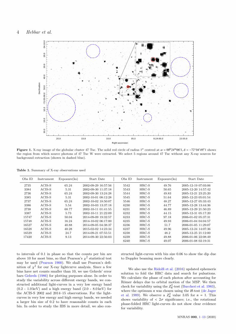
in order to create new level=1 event and badpixel files us-ing the latest calibrations. In order to prevent good eventsfrom being removed, the parameter ‘check_vf_pha’ was setto “no”. The ‘pixel_adj’ parameter was set to “default”(EDSER) in order to obtain the maximal spatial resolution.The X-ray photons corresponding to 47 Tuc W were ex-tracted from a circular region of 1” radius around the source(α = 00h24m06.s1; δ = −72◦04′49.′′1) as shown in Fig. 1. Thisregion was selected as a compromise between selecting max-imum photons from the target, and avoiding photons fromthe neighbouring source W32. Photons were corrected forbarycentric shifts using the axbary tool of CIAO. The as-pect solution file and the exposure statistics file were alsocorrected in order to correct the good time intervals. Fiveregions close to 47 Tuc, and free of sources, were chosen forbackground subtraction, and barycentric correction was alsoapplied to the background lightcurves.

2.2 Optical Observations

We use the reduced, folded optical and UV data as presentedin Bogdanov et al. (2005) and Cadelano et al. (2015) for ouranalysis. Hubble Space Telescope observations of 47 Tuc re-veal the optical light-curve of the companion star. Bogdanovet al. (2005) plot the optical light-curves in the ACS bandsF435W (67 points), F475W (19 points), F555W (8 points)and F606W (6 points), but only as normalised fluxes as afunction of an unpublished radio ephemeris. However, theyalso plot fluxes in these four bands with the SED of thecompanion at maximum, and from this we can estimate thefluxes of the individual detections. Cadelano et al. (2015)plotted WFC3 F300X (12 points) and F390W (5 points)magnitudes (on the HST system) as a function of binaryphase on an updated radio ephemeris by P. Freire. We di-rect readers to the above mentioned papers for details of theoptical data reduction methods.

2.3 X-ray orbital and spin variability analyses

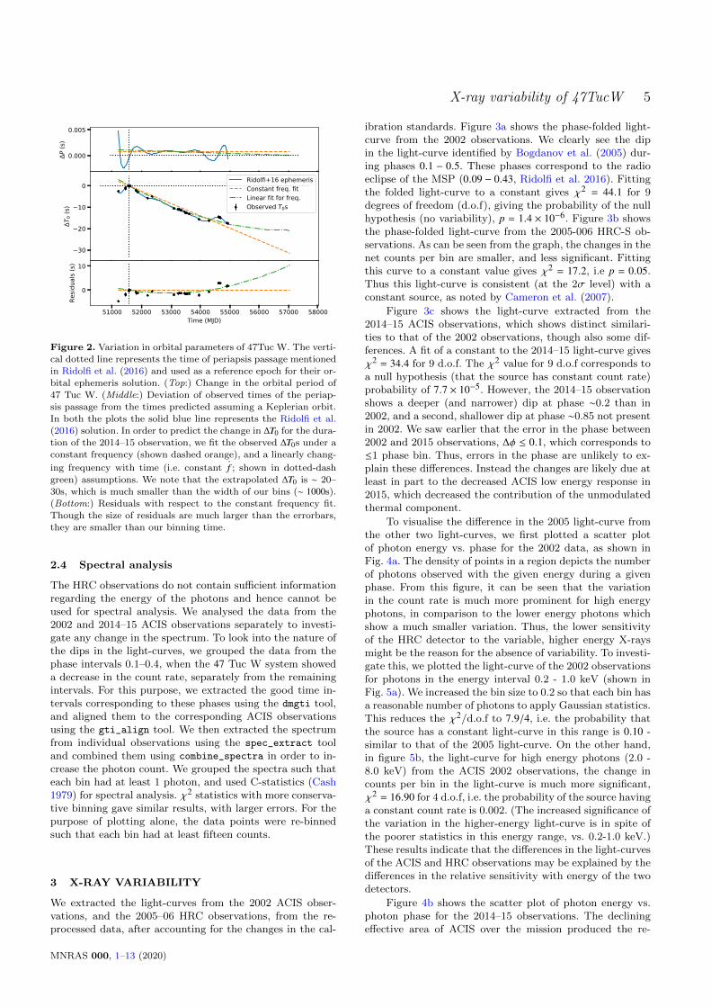
We used the ephemeris data of 47 Tuc W from Ridolfi et al.(2016) to prepare the phase folded X-ray light-curve. How-ever, this ephemeris contains many derivatives, and thus di-verges for times (such as our 2015 epoch) outside the epochsover which it is defined (February 5, 1999 to April 13, 2009).However, in Fig. 2 (plotted from February 5, 1999 to Febru-ary 3, 2015), we see that the change in time of passage ofperiapsis changes by . 20 s across ∼ 11 years (the durationover which the radio pulses were observed). Extrapolatingthis to the epoch of our 2015 data, we see that the changein ∆T0 ∼ 20− 30 s, which is much less than the time intervalcorresponding to our phase bins (∼ 1000 s). Thus we usethe orbital frequency of Ridolfi et al. (2016) without anymodification.

We then constructed phase-folded light-curves in theenergy interval 0.3 − 8.0 keV separately for each observa-tion from the corresponding barycentre-corrected source andbackground files using the dmtcalc and dmextract com-mands. We created phase-folded light-curves for observa-tions taken in 2002, 2005–06 and 2014–15 separately. Thisenables us to study any possible differences in the light-curves across the three epochs. We binned the light-curves

MNRAS 000, 1–13 (2020)

4 Hebbar et al.

Figure 1. X-ray image of the globular cluster 47 Tuc. The solid red circle of radius 1′′ centred at α = 00h24m06.s1, δ = −72◦04′49.′′1 showsthe region from which source photons of 47 Tuc W were extracted. We select 5 regions around 47 Tuc without any X-ray sources for

background extraction (shown in dashed blue).

Table 1. Summary of X-ray observations used

Obs ID Instrument Exposure(ks) Start Date Obs ID Instrument Exposure(ks) Start Date

2735 ACIS-S 65.24 2002-09-29 16:57:56 5542 HRC-S 49.76 2005-12-19 07:03:063384 ACIS-S 5.31 2002-09-30 11:37:18 5543 HRC-S 50.65 2005-12-20 14:57:42

2736 ACIS-S 65.24 2002-09-30 13:24:28 5544 HRC-S 49.83 2005-12-21 23:25:20

3385 ACIS-S 5.31 2002-10-01 08:12:28 5545 HRC-S 51.64 2005-12-23 05:01:542737 ACIS-S 65.24 2002-10-02 18:50:07 5546 HRC-S 48.27 2005-12-27 05:33:433386 ACIS-S 5.54 2002-10-03 13:37:18 6230 HRC-S 44.77 2005-12-28 13:44:36

2738 ACIS-S 68.77 2002-10-11 01:41:55 6231 HRC-S 46.89 2005-12-29 21:50:233387 ACIS-S 5.73 2002-10-11 21:22:09 6232 HRC-S 44.15 2005-12-31 05:17:20

15747 ACIS-S 50.04 2014-09-09 19:32:57 6233 HRC-S 97.18 2006-01-02 05:37:31

15748 ACIS-S 16.24 2014-10-02 06:17:00 6235 HRC-S 49.93 2006-01-04 04:04:5716527 ACIS-S 40.88 2014-09-05 04:38:37 6236 HRC-S 51.7 2006-01-05 11:29:07

16528 ACIS-S 40.28 2015-02-02 14:23:34 6237 HRC-S 49.96 2005-12-24 14:07:3616529 ACIS-S 24.7 2014-09-21 07:55:51 6238 HRC-S 48.2 2005-12-25 21:12:00

17420 ACIS-S 9.13 2014-09-30 22:56:03 6239 HRC-S 49.88 2006-01-06 22:08:49

6240 HRC-S 49.07 2006-01-08 02:19:31

to intervals of 0.1 in phase so that the counts per bin areabove 10 for most bins, so that Pearson’s χ2 statistical testmay be used (Pearson 1900). We shall use Pearson’s defi-nition of χ2 for our X-ray lightcurve analysis. Since a fewbins have net counts smaller than 10, we use Gehrels’ errorbars Gehrels (1986) for plotting purposes alone. In order tostudy the variability across different energy bands, we con-structed additional light-curves in a very low energy band(0.2 - 1.0 keV) and a high energy band (2.0 - 8.0 keV) forthe ACIS-S 2002 and 2014–15 observations. For the light-curves in very low energy and high energy bands, we neededa larger bin size of 0.2 to have reasonable counts in eachbin. In order to study the IBS in more detail, we also con-

structed light-curves with bin size 0.06 to show the dip dueto Doppler beaming more clearly.

We also use the Ridolfi et al. (2016) updated ephemerissolution to fold the HRC data and search for pulsations.We calculate the phase of each photon after accounting forRomer delays due to orbital motion of the MSP. We thencheck for variability using the Z2

n-test (Buccheri et al. 1983),where the optimum n was chosen using the H-test (de Jageret al. 1989). We observe a Z2

n value 3.05 for n = 1. Thisshows variability of < 2σ significance; i.e., the rotationalphase-folded HRC light-curves do not show clear evidencefor variability.

MNRAS 000, 1–13 (2020)

X-ray variability of 47TucW 5

0.000

0.005

P (s

)

30

20

10

0

T 0 (s

)

Ridolfi+16 ephemerisConstant freq. fitLinear fit for freq.Observed T0s

51000 52000 53000 54000 55000 56000 57000 58000Time (MJD)

0

10

Resid

uals

(s)

Figure 2. Variation in orbital parameters of 47Tuc W. The verti-

cal dotted line represents the time of periapsis passage mentioned

in Ridolfi et al. (2016) and used as a reference epoch for their or-bital ephemeris solution. (Top:) Change in the orbital period of

47 Tuc W. (Middle:) Deviation of observed times of the periap-

sis passage from the times predicted assuming a Keplerian orbit.In both the plots the solid blue line represents the Ridolfi et al.

(2016) solution. In order to predict the change in ∆T0 for the dura-

tion of the 2014–15 observation, we fit the observed ∆T0s under aconstant frequency (shown dashed orange), and a linearly chang-

ing frequency with time (i.e. constant Ûf ; shown in dotted-dashgreen) assumptions. We note that the extrapolated ∆T0 is ∼ 20–

30s, which is much smaller than the width of our bins (∼ 1000s).

(Bottom:) Residuals with respect to the constant frequency fit.Though the size of residuals are much larger than the errorbars,

they are smaller than our binning time.

2.4 Spectral analysis

The HRC observations do not contain sufficient informationregarding the energy of the photons and hence cannot beused for spectral analysis. We analysed the data from the2002 and 2014–15 ACIS observations separately to investi-gate any change in the spectrum. To look into the nature ofthe dips in the light-curves, we grouped the data from thephase intervals 0.1–0.4, when the 47 Tuc W system showeda decrease in the count rate, separately from the remainingintervals. For this purpose, we extracted the good time in-tervals corresponding to these phases using the dmgti tool,and aligned them to the corresponding ACIS observationsusing the gti_align tool. We then extracted the spectrumfrom individual observations using the spec_extract tooland combined them using combine_spectra in order to in-crease the photon count. We grouped the spectra such thateach bin had at least 1 photon, and used C-statistics (Cash1979) for spectral analysis. χ2 statistics with more conserva-tive binning gave similar results, with larger errors. For thepurpose of plotting alone, the data points were re-binnedsuch that each bin had at least fifteen counts.

3 X-RAY VARIABILITY

We extracted the light-curves from the 2002 ACIS obser-vations, and the 2005–06 HRC observations, from the re-processed data, after accounting for the changes in the cal-

ibration standards. Figure 3a shows the phase-folded light-curve from the 2002 observations. We clearly see the dipin the light-curve identified by Bogdanov et al. (2005) dur-ing phases 0.1 − 0.5. These phases correspond to the radioeclipse of the MSP (0.09 − 0.43, Ridolfi et al. 2016). Fittingthe folded light-curve to a constant gives χ2 = 44.1 for 9degrees of freedom (d.o.f), giving the probability of the nullhypothesis (no variability), p = 1.4 × 10−6. Figure 3b showsthe phase-folded light-curve from the 2005-006 HRC-S ob-servations. As can be seen from the graph, the changes in thenet counts per bin are smaller, and less significant. Fittingthis curve to a constant value gives χ2 = 17.2, i.e p = 0.05.Thus this light-curve is consistent (at the 2σ level) with aconstant source, as noted by Cameron et al. (2007).

Figure 3c shows the light-curve extracted from the2014–15 ACIS observations, which shows distinct similari-ties to that of the 2002 observations, though also some dif-ferences. A fit of a constant to the 2014–15 light-curve givesχ2 = 34.4 for 9 d.o.f. The χ2 value for 9 d.o.f corresponds toa null hypothesis (that the source has constant count rate)probability of 7.7 × 10−5. However, the 2014–15 observationshows a deeper (and narrower) dip at phase ∼0.2 than in2002, and a second, shallower dip at phase ∼0.85 not presentin 2002. We saw earlier that the error in the phase between2002 and 2015 observations, ∆φ ≤ 0.1, which corresponds to≤1 phase bin. Thus, errors in the phase are unlikely to ex-plain these differences. Instead the changes are likely due atleast in part to the decreased ACIS low energy response in2015, which decreased the contribution of the unmodulatedthermal component.

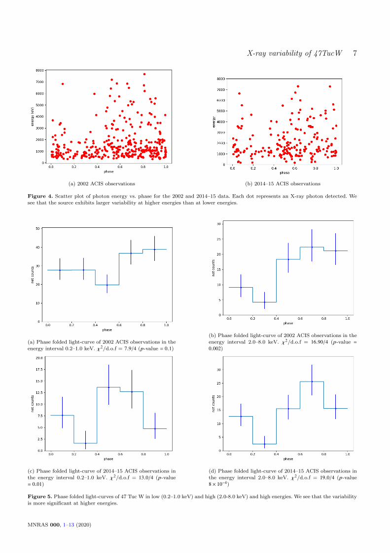
To visualise the difference in the 2005 light-curve fromthe other two light-curves, we first plotted a scatter plotof photon energy vs. phase for the 2002 data, as shown inFig. 4a. The density of points in a region depicts the numberof photons observed with the given energy during a givenphase. From this figure, it can be seen that the variationin the count rate is much more prominent for high energyphotons, in comparison to the lower energy photons whichshow a much smaller variation. Thus, the lower sensitivityof the HRC detector to the variable, higher energy X-raysmight be the reason for the absence of variability. To investi-gate this, we plotted the light-curve of the 2002 observationsfor photons in the energy interval 0.2 - 1.0 keV (shown inFig. 5a). We increased the bin size to 0.2 so that each bin hasa reasonable number of photons to apply Gaussian statistics.This reduces the χ2/d.o.f to 7.9/4, i.e. the probability thatthe source has a constant light-curve in this range is 0.10 -similar to that of the 2005 light-curve. On the other hand,in figure 5b, the light-curve for high energy photons (2.0 -8.0 keV) from the ACIS 2002 observations, the change incounts per bin in the light-curve is much more significant,χ2 = 16.90 for 4 d.o.f, i.e. the probability of the source havinga constant count rate is 0.002. (The increased significance ofthe variation in the higher-energy light-curve is in spite ofthe poorer statistics in this energy range, vs. 0.2-1.0 keV.)These results indicate that the differences in the light-curvesof the ACIS and HRC observations may be explained by thedifferences in the relative sensitivity with energy of the twodetectors.

Figure 4b shows the scatter plot of photon energy vs.photon phase for the 2014–15 observations. The decliningeffective area of ACIS over the mission produced the re-

MNRAS 000, 1–13 (2020)

6 Hebbar et al.

(a) Orbital phase-folded light-curve of 47 Tuc W from ACIS

2002 observations. χ2/d.o.f = 44.1/9 (p-value = 1.4 × 10−6).

(b) Orbital phase-folded light-curve of 47 Tuc W from HRC

2005–06 observations. χ2/d.o.f = 17.2/9 (p-value = 0.05).

(c) Orbital phase-folded light-curve of 47 Tuc W from ACIS2014–15 observations. χ2/d.o.f = 34.4/9 (p-value = 7.7×10−5).

(d) Cumulative distribution of photons from the 2002, 2005–

06, and 2014–15 observations. Uniform distribution is alsoplotted for comparison.

Figure 3. X-ray light-curve analysis of 47 Tuc W. We observe that the net count rate in 2002 and 2014–15 ACIS light-curves (extracted

in the 0.3–8.0 keV energy range) decreases during phase interval 0.1–0.4. However the light-curve from 2005–06 HRC data does not

show variability. We also show the cumulative distribution of the photons during the three observations to give an unbinned perspectiveand compare them to a uniform distribution (constant net count-rate). Performing the Kolmogorov-Smirnov test (KS test) between the

unbinned light-curves and a uniform distribution gives values 0.17 (p−value = 1.2 × 10−8) for 2002 data, 0.16 (p−value = 1.7 × 10−4) for

the 2015 data, and 0.063 (p−value = 0.032 i.e < 3σ confidence) for the 2005 data.

duced number of low energy photons in Fig. 4b, comparedto Fig. 4a. Figs. 5c, 5d show the low and high energy light-curves for the 2014–15 observations. The 2014–15 observa-tions show a less dramatic difference in the variability char-acteristics of low and high-energy photons, largely becausethe lowest-energy photons are simply missing in 2014–15(compare Fig. 4b and Fig. 4a). The high energy light-curvesof 2002 and 2014–15 observations are similar.

4 X-RAY SPECTRUM

We analysed the X-ray spectrum for 47 Tuc W using the0.3 - 8.0 keV photons where the ACIS instrument has thehighest sensitivity. We divided the data into 4 groups to lookfor changes in the spectra during eclipse, and between the2002 and 2014–15 observations:

• D1 - Data from 2002 observations extracted fromphases 0.0-0.1, and 0.4- 1.0 (higher flux).

• D2 - Data from 2014–15 observations extracted fromphases 0.0-0.1, and 0.4- 1.0 (higher flux).

• D3 - Data from 2002 observations extracted fromphases 0.1-0.4 (lower flux).

• D4 - Data from 2014–15 observations extracted fromphases 0.1-0.4 (lower flux).

Due to the low photon counts, we grouped the data tohave a minimum of 1 photon per bin, and used C-statisticsto fit the models. We used the tbabs model in XSPEC tomodel the absorption due to the interstellar medium. Wefixed the hydrogen column density towards 47 Tuc to be3.5 × 1020 cm−2 (Bogdanov et al. 2016), using wilms abun-dances (Wilms et al. 2000). We describe the various spectralmodels used and the approximations made in the paragraphs

MNRAS 000, 1–13 (2020)

X-ray variability of 47TucW 7

(a) 2002 ACIS observations (b) 2014–15 ACIS observations

Figure 4. Scatter plot of photon energy vs. phase for the 2002 and 2014–15 data. Each dot represents an X-ray photon detected. We

see that the source exhibits larger variability at higher energies than at lower energies.

(a) Phase folded light-curve of 2002 ACIS observations in the

energy interval 0.2–1.0 keV. χ2/d.o.f = 7.9/4 (p-value = 0.1)

(b) Phase folded light-curve of 2002 ACIS observations in theenergy interval 2.0–8.0 keV. χ2/d.o.f = 16.90/4 (p-value =

0.002)

(c) Phase folded light-curve of 2014–15 ACIS observations in

the energy interval 0.2–1.0 keV. χ2/d.o.f = 13.0/4 (p-value

= 0.01)

(d) Phase folded light-curve of 2014–15 ACIS observations in

the energy interval 2.0–8.0 keV. χ2/d.o.f = 19.0/4 (p-value

8 × 10−4)

Figure 5. Phase folded light-curves of 47 Tuc W in low (0.2–1.0 keV) and high (2.0-8.0 keV) and high energies. We see that the variabilityis more significant at higher energies.

MNRAS 000, 1–13 (2020)

8 Hebbar et al.

Figure 6. Spectral fits to the 2002 data (black: bright, phases

-0.0-0.1, 0.4-1.0; red: faint, phases - 0.1-0.4), and 2014–15 data(green: bright, phases phases - 0.0-0.1, 0.4-1.0. blue: faint, phases

0.1-0.4). Top: Model with power-law and blackbody components,

and tbabs absorption. Bottom: Model with power-law and neu-tron star atmosphere components, plus absorption. We also plot

the thermal (dotted) and non-thermal (dashed) components ofthe spectrum separately for the 2002 bright (black) and faint (red)

spectra.

below. The results of our spectral analysis are summarisedin Table 2. We quote 90% confidence errorbars.

We first fit all four data groups independently with apower law (model 1). Due to the low photon counts, theparameters of the spectral fits for D3 and D4 were essentiallyunconstrained. We observed that the photon indices of D1and D2 were consistent within their 90% confidence errors,as were those of D3 and D4. Therefore, we linked the photonindices of (D1, D2) and (D3, D4) to be equal. Fitting apegged power law, with linked photon indices (model 2),gave Γ = 1.49 ± 0.12 for D1 and D2 (the bright phases) andΓ = 2.31 ± 0.32 for D3 and D4 (the faint phases).

The large change in the photon index during the fluxdips suggests the possibility of two spectral components in47 Tuc W. The hard spectrum could be emitted from theintra-binary shock (IBS). The decrease in flux from this hardspectral component could be due to eclipsing by the compan-ion, or due to Doppler beaming of radiation from the shockedmaterial away from us. The softer spectrum could be ther-mal emission from the NS, which would not be eclipsed by

the companion except at very high inclinations (and thenonly for a very short phase interval). The soft spectrum fromthe NS could be fit by either a blackbody (BB) (model 3)or a neutron star atmosphere (nsatmos, Heinke et al. 2006)model (model 4). We assumed the emission from the neu-tron star to be constant with phase, as the inclination isunlikely to be large enough for a direct occultation of theNS by the small secondary (which would be very short evenif it occurred, <5% of the orbit). Therefore we assume thatthe parameters of the softer spectrum are constant acrossall the data groups. Note that since there could be someX-ray emission from the IBS, even during the phases whereflux decreases, we do not fix the power-law flux to be zeroin data groups D3 and D4.

We modelled the BB emission using bbodyrad inXSPEC, limiting the BB temperature to <0.3 keV (to avoidthe fit increasing the BB temperature to fit the high-energycomponent). We kept the BB component parameters identi-cal across the 4 data groups, and allowed only the power-lawcomponent normalisation to vary between the data groups.Including the thermal component decreases the power-lawindex slightly to Γ = 1.16+0.24

−0.26. The BB component has an

effective temperature Te f f = 1.84+0.48−0.58 × 106 K, and a radius

Re f f = 0.24+0.27−0.09 km - consistent with emission from heated

polar caps of a NS, as seen in other MSPs (e.g. Bogdanovet al. 2006). From the best fit model (Fig. 6 (top), we seethat the non-thermal flux is roughly twice the thermal fluxeven during the phase interval 0.1-0.4.

We also fit the soft component with a neutron star at-mosphere, using the nsatmos model of XSPEC. We fix theneutron star mass to 1.4 M�, the neutron star radius to 10km, and the distance to 4.53 kpc (Bogdanov et al. 2016).The norm parameter in this model allows a rough estimateof the fractional part of the neutron star emitting, whichwe left free, but tied to the same value between the datagroups (model 4). The radius of the region emitting thermalradiation is much smaller than the NS radius, indicating thepresence of hot spots on the NS. Fixing the norm to 1 andvarying the radius of the NS gives an extremely small radius(∼ 5 km), which is not plausible.

The best fitting model shown in Fig. 6 (bottom),has a photon index Γ = 1.04+0.26

−0.27, similar to that in thetbabs*(pegpwrlw+bbodyrad) model. We find that the tem-perature and radius of the hotspot on the NS are 1.05+0.36

−0.37 ×106 K and 1.29+1.61

−0.49 km, respectively. These are again con-sistent with the values for NS hotspots in other MSPs (e.g.Bogdanov et al. 2006). Since nsatmos is a more physicallymotivated model for emission from a neutron star surface,we use this model for further analysis.

From Table 2, we see that the thermal flux is muchsmaller (≈ 1/5) than the non-thermal one outside dips.The non-thermal and thermal luminosities are estimated asLX,NT = (2.5 ± 0.4) × 1031 ergs/s, and LX,NS = 5+1

−2 × 1030

ergs/s between 0.3 - 8.0 keV for the 2002 data. The non-thermal flux seems to have increased during the 2014–15observations, compared to the 2002 observations. We ver-ify this change in the power-law flux using two methods —First, we tie the power-law flux of (D1, D2) and (D3, D4),and check the change in C-statistic value. This increases theC-statistic by 9.07 while decreasing the d.o.f by 2, i.e. thep-value = 0.01 for constant flux. Next, we use the model

MNRAS 000, 1–13 (2020)

X-ray variability of 47TucW 9

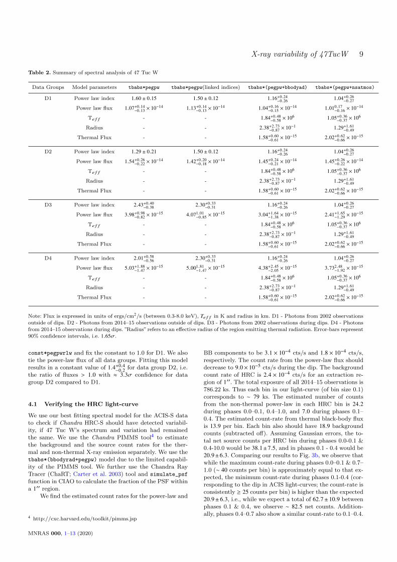
Table 2. Summary of spectral analysis of 47 Tuc W

Data Groups Model parameters tbabs*pegpw tbabs*pegpw(linked indices) tbabs*(pegpw+bbodyad) tbabs*(pegpw+nsatmos)

D1 Power law index 1.60 ± 0.15 1.50 ± 0.12 1.16+0.24−0.26 1.04+0.26

−0.27

Power law flux 1.07+0.14−0.13 × 10−14 1.13+0.14

−0.13 × 10−14 1.04+0.16−0.15 × 10−14 1.010.17

−0.16 × 10−14

Te f f - - 1.84+0.48−0.58 × 106 1.05+0.36

−0.37 × 106

Radius - - 2.38+2.73−0.87 × 10−1 1.29+1.61

−0.49

Thermal Flux - - 1.58+0.60−0.61 × 10−15 2.02+0.62

−0.66 × 10−15

D2 Power law index 1.29 ± 0.21 1.50 ± 0.12 1.16+0.24−0.26 1.04+0.26

−0.27

Power law flux 1.54+0.26−0.22 × 10−14 1.42+0.20

−0.18 × 10−14 1.45+0.24−0.21 × 10−14 1.45+0.26

−0.22 × 10−14

Te f f - - 1.84+0.48−0.58 × 106 1.05+0.36

−0.37 × 106

Radius - - 2.38+2.73−0.87 × 10−1 1.29+1.61

−0.49

Thermal Flux - - 1.58+0.60−0.61 × 10−15 2.02+0.62

−0.66 × 10−15

D3 Power law index 2.43+0.40−0.38 2.30+0.33

−0.31 1.16+0.24−0.26 1.04+0.26

−0.27

Power law flux 3.98+0.98−0.82 × 10−15 4.071.01

−0.85 × 10−15 3.04+1.64−1.38 × 10−15 2.41+1.65

−1.29 × 10−15

Te f f - - 1.84+0.48−0.58 × 106 1.05+0.36

−0.37 × 106

Radius - - 2.38+2.73−0.87 × 10−1 1.29+1.61

−0.49

Thermal Flux - - 1.58+0.60−0.61 × 10−15 2.02+0.62

−0.66 × 10−15

D4 Power law index 2.01+0.58−0.56 2.30+0.33

−0.31 1.16+0.24−0.26 1.04+0.26

−0.27

Power law flux 5.03+1.88−1.47 × 10−15 5.001.81

−1.47 × 10−15 4.38+2.45−2.05 × 10−15 3.732.48

−1.92 × 10−15

Te f f - - 1.84+0.48−0.58 × 106 1.05+0.36

−0.37 × 106

Radius - - 2.38+2.73−0.87 × 10−1 1.29+1.61

−0.49

Thermal Flux - - 1.58+0.60−0.61 × 10−15 2.02+0.62

−0.66 × 10−15

Note: Flux is expressed in units of ergs/cm2/s (between 0.3-8.0 keV), Te f f in K and radius in km. D1 - Photons from 2002 observations

outside of dips. D2 - Photons from 2014–15 observations outside of dips. D3 - Photons from 2002 observations during dips. D4 - Photonsfrom 2014–15 observations during dips. ”Radius” refers to an effective radius of the region emitting thermal radiation. Error-bars represent

90% confidence intervals, i.e. 1.65σ.

const*pegpwrlw and fix the constant to 1.0 for D1. We alsotie the power-law flux of all data groups. Fitting this modelresults in a constant value of 1.4+0.4

−0.2 for data group D2, i.e.the ratio of fluxes > 1.0 with ≈ 3.3σ confidence for datagroup D2 compared to D1.

4.1 Verifying the HRC light-curve

We use our best fitting spectral model for the ACIS-S datato check if Chandra HRC-S should have detected variabil-ity, if 47 Tuc W’s spectrum and variation had remainedthe same. We use the Chandra PIMMS tool4 to estimatethe background and the source count rates for the ther-mal and non-thermal X-ray emission separately. We use thetbabs*(bbodyrad+pegpw) model due to the limited capabil-ity of the PIMMS tool. We further use the Chandra RayTracer (ChaRT; Carter et al. 2003) tool and simulate_psf

function in CIAO to calculate the fraction of the PSF withina 1′′ region.

We find the estimated count rates for the power-law and

4 http://cxc.harvard.edu/toolkit/pimms.jsp

BB components to be 3.1 × 10−4 cts/s and 1.8 × 10−4 cts/s,respectively. The count rate from the power-law flux shoulddecrease to 9.0× 10−5 cts/s during the dip. The backgroundcount rate of HRC is 2.4 × 10−4 cts/s for an extraction re-gion of 1′′. The total exposure of all 2014–15 observations is786.22 ks. Thus each bin in our light-curve (of bin size 0.1)corresponds to ∼ 79 ks. The estimated number of countsfrom the non-thermal power-law in each HRC bin is 24.2during phases 0.0–0.1, 0.4–1.0, and 7.0 during phases 0.1–0.4. The estimated count-rate from thermal black-body fluxis 13.9 per bin. Each bin also should have 18.9 backgroundcounts (subtracted off). Assuming Gaussian errors, the to-tal net source counts per HRC bin during phases 0.0-0.1 &0.4-10.0 would be 38.1±7.5, and in phases 0.1 - 0.4 would be20.9±6.3. Comparing our results to Fig. 3b, we observe thatwhile the maximum count-rate during phases 0.0–0.1 & 0.7–1.0 (∼ 40 counts per bin) is approximately equal to that ex-pected, the minimum count-rate during phases 0.1-0.4 (cor-responding to the dip in ACIS light-curves; the count-rate isconsistently ≥ 25 counts per bin) is higher than the expected20.9± 6.3, i.e., while we expect a total of 62.7± 10.9 betweenphases 0.1 & 0.4, we observe ∼ 82.5 net counts. Addition-ally, phases 0.4–0.7 also show a similar count-rate to 0.1–0.4.

MNRAS 000, 1–13 (2020)

10 Hebbar et al.

Thus, the intra-binary shock in the 47 Tuc W system couldhave intrinsically changed between the 2002 ACIS and the2005 HRC observations.

5 COMPARISON BETWEEN INTRA-BINARYSHOCK MODELS AND X-RAY ANDOPTICAL DATA

In this section, we compile optical and X-ray lightcurves,describe our intra-binary shock model, and explain resultsfrom our fitting.

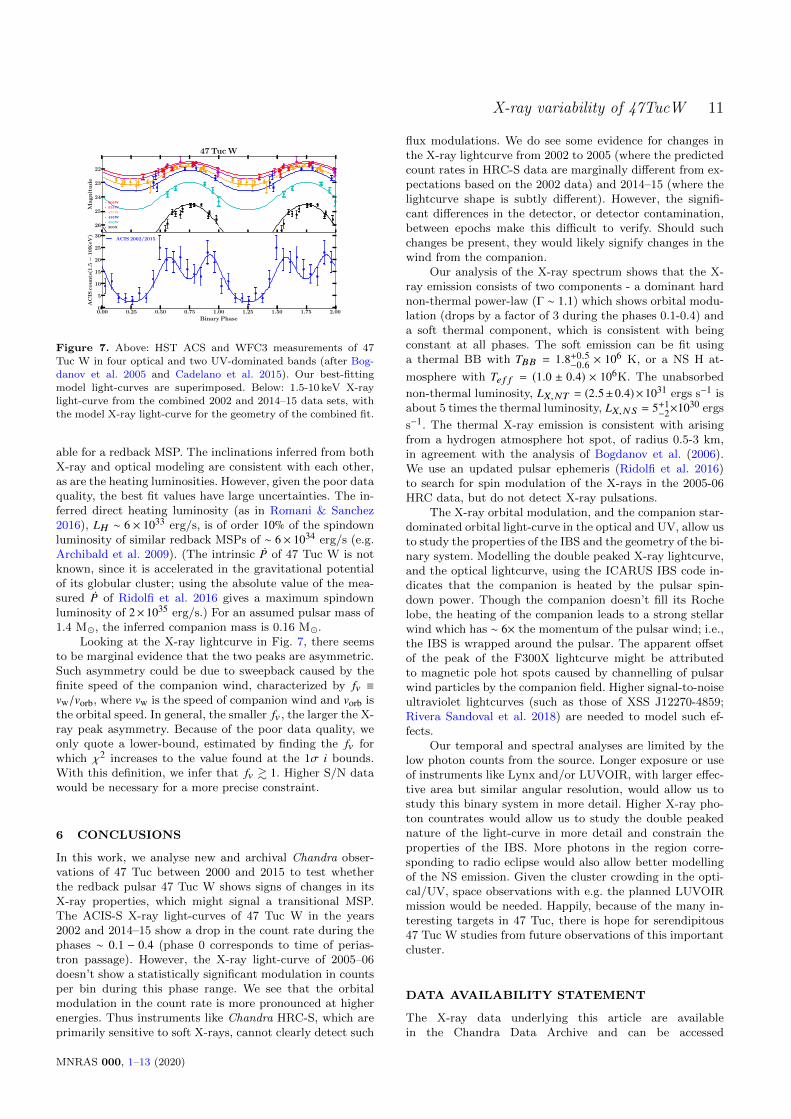
5.1 X-ray and optical data

To model the non-thermal peaks of IBS emission we createda 1.5-10 keV ACIS light-curve. Given that a non-binned KStest shows no significant difference in the phase structureof the 1.5-10 keV counts for the two epochs ((KS test value0.15, p-value = 0.14), we combined the 2002 and 2015 datasets, folding on the orbital period of Ridolfi et al. (2016). TheX-ray maximum is broad, covering over half of the orbit,φB ≈ 0.45 − 0.10, with a hint of a double peak structure(φp,1 ≈ 0.58, φp,2 ≈ 0.93) bracketing the optical maximum(Fig. 7). The radio eclipse covers φB = 0.09 − −0.43 (Ridolfiet al. 2016).

We converted the normalised optical fluxes and errors inBogdanov et al. (2005) and the ultraviolet magnitudes anderrors in Cadelano et al. (2015) to units of erg/cm2/s/Hz( fν) and plot them in Fig. 7 (two periods are shown forclarity). As expected for a cool, heated companion, the op-tical light-curves show relatively shallow dips, while the UVlight-curves show a deeper modulation from the higher tem-perature of the heated part of the companion near the L1point.

All optical/UV light-curves show a maximum near φB ∼0.75 (φB = 0 denotes the phase of the pulsar ascending node),indicating strong heating of the pulsar companion. Severallight-curves appear slightly asymmetric, with the UV curvesdelayed; F300X appears to show a maximum at φB ≈ 0.8. Itis unclear if the offset is significant, but if real it may indicateasymmetric local heating as inferred for other redback-typebinaries. For example, IBS-accelerated particles may con-tribute to the heating, being“ducted”by companion fields tothe surface and producing heated magnetic poles (Sanchez& Romani 2017); this would most strongly affect the UVlight-curves. Similarly, asymmetries in the lightcurves couldalso arise from atmospheric circulations on the surface of thecompanion (Kandel & Romani 2020).

5.2 Intra-binary shock modeling

To model the companion heating, we use the ICARUS codeof Breton et al. (2012). This requires tables of stellar at-mosphere colours as a function of local surface temperatureand gravity. We extract these from the Spanish Virtual Ob-servatory fold of the BT-Settl atmosphere models (Allardet al. 2012) through the responses of the individual HSTfilters, convert the normalized surface fluxes to fν , and sup-ply them to the ICARUS code. The four optical bands showshallow modulation. The five F390W points are puzzling,with our models over-predicting this flux by a factor of 2×,

although the shape is as expected. We suspect that there is adifference between the calibration of Cadelano et al. (2015),and our filter assumptions, although we have not been ableto identify a specific error. The F300X fluxes follow the ex-pected light-curve quite closely. To deal with this we adopta simple offset in the F390W magnitudes.

The non-thermal X-ray emission is attributed to syn-chrotron emission (Bogdanov et al. 2005; Wadiasingh et al.2018) from particles accelerated by the intra-binary shockformed by the interaction of the pulsar wind and the stellarwind from the main-sequence companion. To study the di-rect X-ray emission from the IBS, we have further extendedthe ICARUS IBS code (Romani & Sanchez 2016) with amodule which follows the variation of the synchrotron emis-sion across the shock (Kandel et al. 2019). In this model,the shape of the IBS is controlled by the wind momentumratio β and a wind velocity asymmetry factor fv . The IBSspectral behavior is controlled by the evolution of the bulkflow speed Γ, the spectral index of the accelerated electronpower-law, and the characteristic magnetic field strength atthe IBS nose (the point of the shock on the line connectingthe two stars).

The X-ray lightcurves of many redback MSPs (such as47 Tuc W) show peaks around pulsar superior conjunction.In the standard modeling scenario, this indicates that themomentum of the massive companion wind dominates overthe momentum of the pulsar wind, β > 1, sweeping the shockback to wrap around the pulsar (Romani & Sanchez 2016;Wadiasingh et al. 2018; Al Noori et al. 2018). For our mod-eling we assume, following Kandel et al. (2019), that theshocked pulsar wind accelerates adiabatically along the IBScontact discontinuity

Γ ≈ 1.1(1 + 0.2

sr0

), (1)

where r0 is the stand-off distance of the shock from the nose,and s is the arc length from the nose of the IBS to theposition of interest along the IBS. We also assume that themagnetic field at the nose of the IBS is 10 G.

For many black widows and redbacks, the IBS syn-chrotron emission dominates over non-thermal X-rays di-rectly from the pulsar. Above 1.5 keV, we expect little tono emission from the NS surface, so we treat the 1.5-10 keVX-rays as produced entirely by the shock. For 47 Tuc W,the relatively hard observed X-ray spectrum (photon index∼ 1.04) implies negligible contribution by the IBS emissionto the flux in the optical/UV bands, which are dominatedby the pulsar-heated face of the companion.

To constrain the system parameters, we have fitted theoptical and X-ray data independently. The optical model issensitive to the binary inclination i, while the X-ray light-curve is sensitive to i and the shock geometry. Recall thatthe F390W points are shifted by a phase-independent offsetfit as ∆m = 0.4 ± 0.05 mag to deal with an apparent calibra-tion error. Fig 7 shows the model-fitted optical and X-raylightcurves, and the fitted parameters are listed in Table 3.Note that the UV phase shift, if real, might be due to particleprecipitation to magnetic poles (Sanchez & Romani 2017),or atmospheric circulation on the companion (Kandel & Ro-mani 2020). However, higher S/N light-curves are needed tomotivate such detailed modeling.

The fitted properties in Table 3 seem generally reason-

MNRAS 000, 1–13 (2020)

X-ray variability of 47TucW 11

22

23

24

25

26

Magn

itu

de

47 Tuc W

606W

555W

475W

435W

390W

300X

0.00 0.25 0.50 0.75 1.00 1.25 1.50 1.75 2.00

Binary Phase

0

5

10

15

20

25

30

AC

ISco

unts

(1.5−

10K

eV

)

ACIS 2002/2015

Figure 7. Above: HST ACS and WFC3 measurements of 47

Tuc W in four optical and two UV-dominated bands (after Bog-

danov et al. 2005 and Cadelano et al. 2015). Our best-fittingmodel light-curves are superimposed. Below: 1.5-10 keV X-ray

light-curve from the combined 2002 and 2014–15 data sets, with

the model X-ray light-curve for the geometry of the combined fit.

able for a redback MSP. The inclinations inferred from bothX-ray and optical modeling are consistent with each other,as are the heating luminosities. However, given the poor dataquality, the best fit values have large uncertainties. The in-ferred direct heating luminosity (as in Romani & Sanchez2016), LH ∼ 6 × 1033 erg/s, is of order 10% of the spindownluminosity of similar redback MSPs of ∼ 6 × 1034 erg/s (e.g.Archibald et al. 2009). (The intrinsic ÛP of 47 Tuc W is notknown, since it is accelerated in the gravitational potentialof its globular cluster; using the absolute value of the mea-sured ÛP of Ridolfi et al. 2016 gives a maximum spindownluminosity of 2× 1035 erg/s.) For an assumed pulsar mass of1.4 M�, the inferred companion mass is 0.16 M�.

Looking at the X-ray lightcurve in Fig. 7, there seemsto be marginal evidence that the two peaks are asymmetric.Such asymmetry could be due to sweepback caused by thefinite speed of the companion wind, characterized by fv ≡vw/vorb, where vw is the speed of companion wind and vorb isthe orbital speed. In general, the smaller fv , the larger the X-ray peak asymmetry. Because of the poor data quality, weonly quote a lower-bound, estimated by finding the fv forwhich χ2 increases to the value found at the 1σ i bounds.With this definition, we infer that fv & 1. Higher S/N datawould be necessary for a more precise constraint.

6 CONCLUSIONS

In this work, we analyse new and archival Chandra obser-vations of 47 Tuc between 2000 and 2015 to test whetherthe redback pulsar 47 Tuc W shows signs of changes in itsX-ray properties, which might signal a transitional MSP.The ACIS-S X-ray light-curves of 47 Tuc W in the years2002 and 2014–15 show a drop in the count rate during thephases ∼ 0.1 − 0.4 (phase 0 corresponds to time of perias-tron passage). However, the X-ray light-curve of 2005–06doesn’t show a statistically significant modulation in countsper bin during this phase range. We see that the orbitalmodulation in the count rate is more pronounced at higherenergies. Thus instruments like Chandra HRC-S, which areprimarily sensitive to soft X-rays, cannot clearly detect such

flux modulations. We do see some evidence for changes inthe X-ray lightcurve from 2002 to 2005 (where the predictedcount rates in HRC-S data are marginally different from ex-pectations based on the 2002 data) and 2014–15 (where thelightcurve shape is subtly different). However, the signifi-cant differences in the detector, or detector contamination,between epochs make this difficult to verify. Should suchchanges be present, they would likely signify changes in thewind from the companion.

Our analysis of the X-ray spectrum shows that the X-ray emission consists of two components - a dominant hardnon-thermal power-law (Γ ∼ 1.1) which shows orbital modu-lation (drops by a factor of 3 during the phases 0.1-0.4) anda soft thermal component, which is consistent with beingconstant at all phases. The soft emission can be fit usinga thermal BB with TBB = 1.8+0.5

−0.6 × 106 K, or a NS H at-

mosphere with Te f f = (1.0 ± 0.4) × 106K. The unabsorbed

non-thermal luminosity, LX,NT = (2.5±0.4)×1031 ergs s−1 isabout 5 times the thermal luminosity, LX,NS = 5+1

−2×1030 ergs

s−1. The thermal X-ray emission is consistent with arisingfrom a hydrogen atmosphere hot spot, of radius 0.5-3 km,in agreement with the analysis of Bogdanov et al. (2006).We use an updated pulsar ephemeris (Ridolfi et al. 2016)to search for spin modulation of the X-rays in the 2005-06HRC data, but do not detect X-ray pulsations.

The X-ray orbital modulation, and the companion star-dominated orbital light-curve in the optical and UV, allow usto study the properties of the IBS and the geometry of the bi-nary system. Modelling the double peaked X-ray lightcurve,and the optical lightcurve, using the ICARUS IBS code in-dicates that the companion is heated by the pulsar spin-down power. Though the companion doesn’t fill its Rochelobe, the heating of the companion leads to a strong stellarwind which has ∼ 6× the momentum of the pulsar wind; i.e.,the IBS is wrapped around the pulsar. The apparent offsetof the peak of the F300X lightcurve might be attributedto magnetic pole hot spots caused by channelling of pulsarwind particles by the companion field. Higher signal-to-noiseultraviolet lightcurves (such as those of XSS J12270-4859;Rivera Sandoval et al. 2018) are needed to model such ef-fects.

Our temporal and spectral analyses are limited by thelow photon counts from the source. Longer exposure or useof instruments like Lynx and/or LUVOIR, with larger effec-tive area but similar angular resolution, would allow us tostudy this binary system in more detail. Higher X-ray pho-ton countrates would allow us to study the double peakednature of the light-curve in more detail and constrain theproperties of the IBS. More photons in the region corre-sponding to radio eclipse would also allow better modellingof the NS emission. Given the cluster crowding in the opti-cal/UV, space observations with e.g. the planned LUVOIRmission would be needed. Happily, because of the many in-teresting targets in 47 Tuc, there is hope for serendipitous47 Tuc W studies from future observations of this importantcluster.

DATA AVAILABILITY STATEMENT

The X-ray data underlying this article are availablein the Chandra Data Archive and can be accessed

MNRAS 000, 1–13 (2020)

12 Hebbar et al.

Parameter Symbol Optical Value X-ray value

Inclination (degrees) i 67.6 ± 12.0 51.64 ± 9.99Roche lobe filling factor f1 0.65 ± 0.03 -

Star temperature (night, K) TN 4973 ± 73 -

Heating luminosity (erg s−1) LH (5.74 ± 0.44) × 1033 (3.45 ± 2.05) × 1033

Wind momentum ratio β - 5.1 ± 0.8Chi-square χ2/ν 104/53 14/12

Table 3. Parameters for fit of IBS to optical & X-ray light-curves.

using the Chandra Search and Retrieval (ChaSeR;https://cda.harvard.edu/chaser/) tool. The Hubble SpaceTelescope optical observations corresponding to theoptical data used in this article are available atthe Mikulski Archive for Space Telescopes (MAST;http://archive.stsci.edu/hst/). The light-curves used in thisarticle are presented in Bogdanov et al. (2005) and Cadelanoet al. (2015).

ACKNOWLEDGEMENTS

We thank A. Ridolfi for giving insights into the evolutionof the binary orbit of 47 Tuc W. COH acknowledges sup-port from NSERC Discovery Grant RGPIN-2016-04602, anda Discovery Accelerator Supplement. DK and RWR weresupported in part by NASA grants 80NSSC17K0024 and80NSSC18K1712.

REFERENCES

Al Noori H., et al., 2018, ApJ, 861, 89

Allard F., Homeier D., Freytag B., 2012, Philosophical Transac-

tions of the Royal Society of London Series A, 370, 2765

Alpar M. A., Cheng A. F., Ruderman M. A., Shaham J., 1982,

Nature, 300, 728

Ambrosino F., et al., 2017, Nature Astronomy, 1, 854

Archibald A. M., et al., 2009, Science, 324, 1411

Archibald A. M., et al., 2015, ApJ, 807, 62

Backer D. C., Kulkarni S. R., Heiles C., Davis M. M., Goss W. M.,

1982, Nature, 300, 615

Bahramian A., et al., 2017, MNRAS, 467, 2199

Bassa C. G., et al., 2014, MNRAS, 441, 1825

Becker W., Trumper J., 1993, Nature, 365, 528

Bednarek W., 2014, A&A, 561, A116

Benvenuto O. G., De Vito M. A., Horvath J. E., 2014, ApJ, 786,

L7

Benvenuto O. G., De Vito M. A., Horvath J. E., 2015, ApJ, 798,44

Bhattacharya D., van den Heuvel E. P. J., 1991, Phys. Rep., 203,

1

Bhattacharya S., Heinke C. O., Chugunov A. I., Freire P. C. C.,Ridolfi A., Bogdanov S., 2017, MNRAS, 472, 3706

Bogdanov S., Halpern J. P., 2015, ApJ, 803, L27

Bogdanov S., Grindlay J. E., van den Berg M., 2005, ApJ, 630,

1029

Bogdanov S., Grindlay J. E., Heinke C. O., Camilo F., Freire P.C. C., Becker W., 2006, ApJ, 646, 1104

Bogdanov S., van den Berg M., Heinke C. O., Cohn H. N., Lugger

P. M., Grindlay J. E., 2010, ApJ, 709, 241

Bogdanov S., Archibald A. M., Hessels J. W. T., Kaspi V. M.,Lorimer D., McLaughlin M. A., Ransom S. M., Stairs I. H.,

2011, ApJ, 742, 97

Bogdanov S., Patruno A., Archibald A. M., Bassa C., Hessels

J. W. T., Janssen G. H., Stappers B. W., 2014, ApJ, 789, 40

Bogdanov S., et al., 2015, ApJ, 806, 148

Bogdanov S., Heinke C. O., Ozel F., Guver T., 2016, ApJ, 831,184

Breton R. P., Rappaport S. A., van Kerkwijk M. H., Carter J. A.,

2012, ApJ, 748, 115

Breton R. P., et al., 2013, ApJ, 769, 108

Buccheri R., et al., 1983, A&A, 128, 245

Cadelano M., Pallanca C., Ferraro F. R., Salaris M., Dalessandro

E., Lanzoni B., Freire P. C. C., 2015, ApJ, 812, 63

Callanan P. J., van Paradijs J., Rengelink R., 1995, ApJ, 439, 928

Cameron P. B., Rutledge R. E., Camilo F., Bildsten L., Ransom

S. M., Kulkarni S. R., 2007, ApJ, 660, 587

Camilo F., Rasio F. A., 2005, in Rasio F. A., Stairs I. H., eds,

Astronomical Society of the Pacific Conference Series Vol. 328,

Binary Radio Pulsars. p. 147 (arXiv:astro-ph/0501226)

Camilo F., Lorimer D. R., Freire P., Lyne A. G., Manchester

R. N., 2000, ApJ, 535, 975

Carter C., Karovska M., Jerius D., Glotfelty K., Beikman S., 2003,

ChaRT: The Chandra Ray Tracer. p. 477

Cash W., 1979, ApJ, 228, 939

Coti Zelati F., et al., 2019, A&A, 622, A211

D’Amico N., Possenti A., Manchester R. N., Sarkissian J., LyneA. G., Camilo F., 2001, ApJ, 561, L89

Djorgovski S., Evans C. R., 1988, ApJ, 335, L61

Edmonds P. D., Gilliland R. L., Camilo F., Heinke C. O., Grindlay

J. E., 2002, ApJ, 579, 741

Freire P. C. C., 2005, in Rasio F. A., Stairs I. H., eds, AstronomicalSociety of the Pacific Conference Series Vol. 328, Binary Radio

Pulsars. p. 405 (arXiv:astro-ph/0404105)

Freire P. C. C., et al., 2017, MNRAS, 471, 857

Gehrels N., 1986, ApJ, 303, 336

Grindlay J. E., Heinke C., Edmonds P. D., Murray S. S., 2001,Science, 292, 2290

Heinke C. O., Grindlay J. E., Edmonds P. D., Cohn H. N., LuggerP. M., Camilo F., Bogdanov S., Freire P. C., 2005, ApJ, 625,796

Heinke C. O., Rybicki G. B., Narayan R., Grindlay J. E., 2006,ApJ, 644, 1090

Hill A. B., et al., 2011, MNRAS, 415, 235

Hui C. Y., et al., 2015, ApJ, 801, L27

Kandel D., Romani R. W., 2020, The Astrophysical Journal, 892,

101

Kandel D., Romani R. W., An H., 2019, ApJ, 879, 73

Kong A. K. H., et al., 2012, ApJ, 747, L3

Li K. L., Kong A. K. H., Takata J., Cheng K. S., Tam P. H. T.,Hui C. Y., Jin R., 2014, ApJ, 797, 111

Lyne A. G., Graham-Smith F., 1990, Pulsar astronomy

Manchester R. N., Lyne A. G., Robinson C., D’Amico N., Bailes

M., Lim J., 1991, Nature, 352, 219

Pan Z., Hobbs G., Li D., Ridolfi A., Wang P., Freire P., 2016,

MNRAS, 459, L26

Papitto A., et al., 2013, Nature, 501, 517

Papitto A., et al., 2019, ApJ, 882, 104

MNRAS 000, 1–13 (2020)

X-ray variability of 47TucW 13

Patruno A., Watts A. L., 2012, preprint, (arXiv:1206.2727)

Pearson K., 1900, The London, Edinburgh, and Dublin Philo-

sophical Magazine and Journal of Science, 50, 157Ridolfi A., et al., 2016, MNRAS, 462, 2918

Rivera Sandoval L., et al., 2018, Monthly Notices of the Royal

Astronomical Society, 476, 1086Roberts M. S. E., 2011, in Burgay M., D’Amico N., Espos-

ito P., Pellizzoni A., Possenti A., eds, American Instituteof Physics Conference Series Vol. 1357, American Institute

of Physics Conference Series. pp 127–130 (arXiv:1103.0819),

doi:10.1063/1.3615095Roberts M. S. E., 2013, in van Leeuwen J., ed., IAU Sympo-

sium Vol. 291, Neutron Stars and Pulsars: Challenges and

Opportunities after 80 years. pp 127–132 (arXiv:1210.6903),doi:10.1017/S174392131202337X

Romani R. W., Sanchez N., 2016, ApJ, 828, 7

Romani R. W., Shaw M. S., 2011, ApJ, 743, L26Roy J., et al., 2015, ApJ, 800, L12

Sanchez N., Romani R. W., 2017, ApJ, 845, 42

Stappers B. W., et al., 2014, ApJ, 790, 39Tendulkar S. P., et al., 2014, ApJ, 791, 77

Wadiasingh Z., Venter C., Harding A. K., Bottcher M., Kilian P.,2018, ApJ, 869, 120

Wijnands R., van der Klis M., 1998, Nature, 394, 344

Wilms J., Allen A., McCray R., 2000, ApJ, 542, 914Zavlin V. E., Pavlov G. G., Sanwal D., Manchester R. N., Trum-

per J., Halpern J. P., Becker W., 2002, ApJ, 569, 894

de Jager O. C., Raubenheimer B. C., Swanepoel J. W. H., 1989,A&A, 221, 180

de Martino D., et al., 2010, A&A, 515, A25

de Martino D., et al., 2013, A&A, 550, A89van Kerkwijk M. H., Breton R. P., Kulkarni S. R., 2011, ApJ,

728, 95

This paper has been typeset from a TEX/LATEX file prepared bythe author.

MNRAS 000, 1–13 (2020)