on the value function of a mixed integer linear...
TRANSCRIPT

On the Value Function of a Mixed Integer LinearOptimization Problem and an Algorithm for its
Construction
Ted K. Ralphs and Anahita Hassanzadeh
Department of Industrial and Systems Engineering, Lehigh University, USA
COR@L Technical Report 14T-004

On the Value Function of a Mixed Integer Linear Optimization
Problem and an Algorithm for its Construction
Ted K. Ralphs∗1 and Anahita Hassanzadeh†1
1Department of Industrial and Systems Engineering, Lehigh University, USA
August 3, 2014
Abstract
This paper addresses the value function of a general mixed integer linear optimization prob-lem (MILP). The value function describes the change in optimal objective value as the right-handside is varied and understanding its structure is central to solving a variety of important classesof optimization problems. We propose a discrete representation of the MILP value function anddescribe a cutting plane algorithm for its construction. We show that this algorithm is finitewhen the set of right-hand sides over which the value function of the associated pure integeroptimization problem is finite is bounded. We explore the structural properties of the MILPvalue function and provide a simplification of the Jeroslow Formula obtained by applying ourresults.
1 Introduction
Understanding and exploiting the structure of the value function of an optimization problem is acritical element of solution methods for a variety of important classes of multi-stage and multi-leveloptimization problems. Previous findings on the value function of a pure integer linear optimiza-tion problem (PILP) have resulted in finite algorithms for constructing it, which have in turnenabled the development of solution methods for two-stage stochastic pure integer optimizationproblems (Schultz et al., 1998; Kong et al., 2006) and certain special cases of bilevel optimizationproblems (Bard, 1991, 1998; S DeNegre, 2011; Dempe et al., 2012). Studies of the value function of ageneral mixed integer linear optimization problem (MILP), however, have not yet led to algorithmicadvances. Algorithms for construction have only been proposed in certain special cases (Guzelsoyand Ralphs, 2006), but no practical characterization is known. By “practical,” we mean a charac-terization and associated representation that is suitable for computation and which we can use toformulate problems in which the value function of a MILP is embedded, e.g., multi-stage stochasticprograms.
In this paper, we extend previous results by demonstrating that the MILP value function hasan underlying discrete structure similar to the PILP value function, even in the general case. This
∗E-mail: [email protected]†E-mail: [email protected]
2
discrete structure emerges from separating the function into discrete and continuous parts, whichin turn enables a representation of the function in terms of two discrete sets. We show that thisrepresentation can be constructed and propose an algorithm for doing so. Both the representationand the algorithm are finite under the assumption that the set of right-hand sides over which therelated PILP value function is finite is bounded.
We consider the value function associated with a nominal MILP instance defined as follows. Thevariables of the instance are indexed on the set N = {1, . . . , n}, with I = {1, . . . , r} denoting theindex set for the integer variables and C = {r+ 1, . . . , n} denoting the index set for the continuousvariables. For any D ⊆ N and a vector y indexed on N , we denote by yD the sub-vector consistingof the corresponding components of y. Similarly, for a matrix M , we denote by MD the sub-matrixconstructed by columns of M that correspond to indices in D. Then, the nominal instance weconsider throughout the paper is given by
zIP = inf(x,y)∈X
c>I x+ c>Cy, (MILP)
where (c>I , c>C)> ∈ Rn is the objective function vector and X = {(x, y) ∈ ZI+×RC+ : AIx+ACy = d}
is the feasible region, described by AI ∈ Qm×r, AC ∈ Qm×(n−r), and d ∈ Rm.A pair of vectors (x, y) ∈ X is called a feasible solution and c>I x+ c>Cy is its associated solution
value. For such a solution, the vector x is referred to as the integer part and the vector y as thecontinuous part. Any (x∗, y∗) ∈ X such that c>I x
∗ + c>Cy∗ = zIP is called an optimal solution.
Throughout the paper, we assume rank(A, d) = rank(A) = m.The value function is a function z : Rm → R ∪ {±∞} that describes the change in the optimal
solution value of a MILP as the right-hand side is varied. In the case of (MILP), we have
z(b) = inf(x,y)∈S(b)
c>I x+ c>Cy ∀b ∈ B, (MVF)
where for b ∈ Rm, S(b) = {(x, y) ∈ Zr+ × Rn−r+ : AIx+ACy = b} and SI(b) = {x ∈ Zr+ : AIx = b}.We let B = {b ∈ Rm : S(b) 6= ∅}, BI = {b ∈ Rm : SI(b) 6= ∅} and SI = ∪b∈BSI(b). By convention,we let z(b) = ∞ for b ∈ Rm \ B and z(b) = −∞ when the infimum in (MVF) is not attained forany x ∈ S(b) for b ∈ B. To simplify the presentation, we assume that z(0) = 0, since otherwisez(b) = −∞ for all b ∈ Rm with S(b) 6= ∅ (Nemhauser and Wolsey, 1988).
To illustrate the basic concepts, we now present a brief example that we refer to throughoutthe paper.
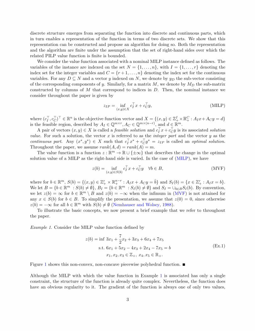
Example 1. Consider the MILP value function defined by
z(b) = inf 3x1 +7
2x2 + 3x3 + 6x4 + 7x5
s.t. 6x1 + 5x2 − 4x3 + 2x4 − 7x5 = b
x1, x2, x3 ∈ Z+, x4, x5 ∈ R+.
(Ex.1)
Figure 1 shows this non-convex, non-concave piecewise polyhedral function.
Although the MILP with which the value function in Example 1 is associated has only a singleconstraint, the structure of the function is already quite complex. Nevertheless, the function doeshave an obvious regularity to it. The gradient of the function is always one of only two values,
3

Figure 1: MILP Value Function of (Ex.1).
which means that its epigraph is the union of a set of polyhedral cones that are identical, asidefrom the location of their extreme points. This allows the function to be represented simply bydescribing this single polyhedral cone and a discrete set of points at which we place translations ofit.
In the remainder of the paper, we formalize the basic idea illustrated in Example 1 and showthat it can be generalized to obtain a similar result that holds for all MILP value functions. Morespecifically, in Section 3, we review some basic properties of the LP value function and define thecontinuous restriction, an LP whose value function yields the aforementioned polyhedral cone. InSections 4, we present the first main result in Theorem 1, which characterizes the minimal discreteset of points that yields a full description of the value function. This discrete set generalizes theminimal tenders of Kong et al. (2006) used to represent the PILP value function. In Section 5,we exploit this representation to uncover further properties of the value function, culminating inTheorem 2, which shows that there is a one-to-one correspondence between the discrete set ofTheorem 1 and the regions over which the value function is convex (the local stability regions). InSection 6, we discuss the relationship of our representation with the well-known Jeroslow Formula,showing in Theorem 3 that the original formula can be simplified using the discrete representation ofTheorem 1. Finally, in Section 7 we demonstrate how to put the representation into computationalpractice by presenting a cutting plane algorithm for constructing a discrete representation such asthe one in Theorem 1 (though possibly not provably minimal). Before getting to the main results,we next summarize related work.
2 Related Work
Much of the recent work on the value function has addressed the pure integer case, since the PILPvalue function has some desirable properties that enable more practical results. Blair and Jeroslow(1982) first showed that the value function of a PILP is a Gomory function that can be derivedby taking the maximum of finitely many subadditive functions. Conti and Traverso (1991) thenproposed using reduced Grobner basis methods to solve PILPs. Subsequently, in the context ofstochastic optimization, Schultz et al. (1998) used the so-called Buchberger Algorithm to compute
4
the reduced Grobner basis for solving sequences of integer optimization problems which differ onlyin their right-hand sides. In the same paper, the authors recognized that over certain regions ofthe right-hand side space, the pure integer value function remains constant. This property turnedout to be quite significant, resulting in algorithms for two-stage stochastic optimization (Ahmedet al., 2004; Kong et al., 2006). In the same vein, Kong et al. (2006) proposed using the propertiesof a pure integer optimization problem in two algorithms for constructing the PILP value functionwhen the set of right-hand sides is finite.
The complex structure of the MILP value function makes the extension of results in linearand pure integer optimization to the general case a challenge. In particular, with the introductionof continuous variables, we no longer have countability of the set of right-hand sides for whichS(b) 6= ∅ (or finiteness in the case of a bounded S(b)), which is a central property in the PILP case.The MILP value function also ostensibly lacks certain properties used in previous algorithms foreliminating parts of the domain from consideration in the pure integer case. For the mixed integercase, Bank et al. (1983) studied the MILP value function in the context of parametric optimizationand provided theoretical results on regions of the right-hand side set over which the function iscontinuous. In a series of papers, Blair and Jeroslow (1977, 1979) studied the properties of theMILP value function and showed that it is a piecewise polyhedral function. Blair and Jeroslow(1984) identified a subclass of Gomory functions called Chvatal functions to which the generalMILP value function belongs. However, a closed form representation was not achieved until adecade later in a subsequent work of Blair (1995). The so-called Jeroslow Formula representsthe MILP value function as collection of Gomory functions with linear correction terms. Thischaracterization is related to ours and we discuss this relationship in Section 6.
3 The Continuous Restriction
To understand the MILP value function, it is important to first understand the structure of thevalue function of a linear optimization problem. In particular, we are interested in the structure ofthe value function of the LP arising from (MILP) by fixing the values of the integer variables. Wecall this problem the continuous restriction (CR) w.r.t a given x ∈ SI . Its value function is givenby
z(b; x) = c>I x+ inf c>Cy
s.t. ACy = b−AI xy ∈ Rn−r+ .
(CR)
For a given x ∈ SI , we let S(b, x) = {y ∈ Rn−r+ : ACy = b − AI x}. As before, we let z(b; x) = ∞if S(b, x) = ∅ for a given b ∈ B and z(b; x) = −∞ if the function value is unbounded. As we willshow formally in Proposition 4, it is evident that for any x ∈ SI , z(·; x) bounds the value functionfrom above, which is the reason for the notation.
When x = 0 in (CR), the resulting function is in fact the value function of a general LP, sinceAC is itself an arbitrary matrix. In the remainder of the section, we consider this important specialcase and define
zC(b) = inf c>Cy
s.t. ACy = b
y ∈ Rn−r+ .
(LVF)
5
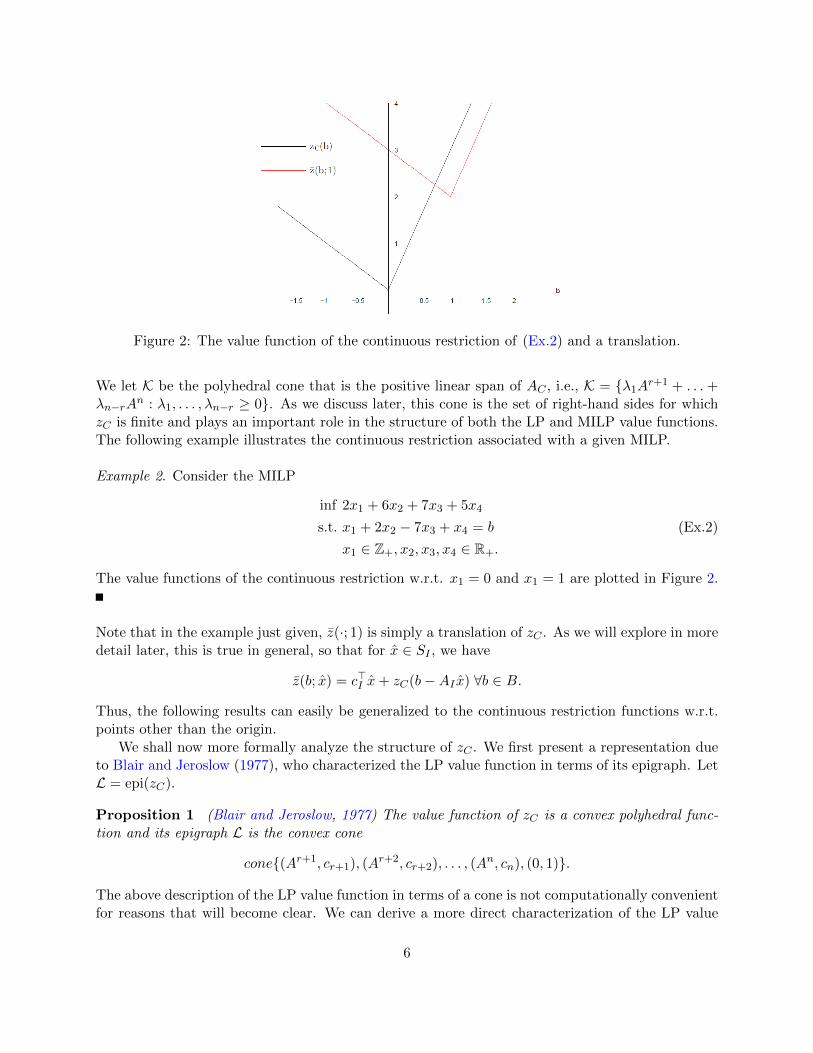
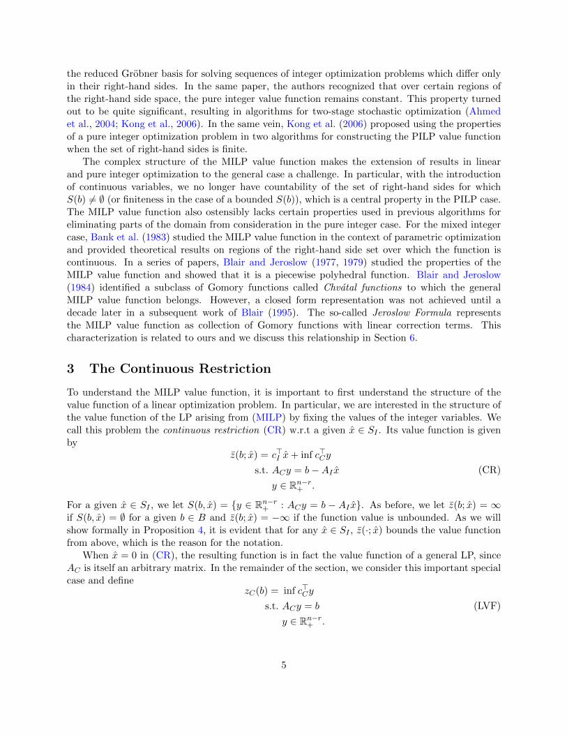
Figure 2: The value function of the continuous restriction of (Ex.2) and a translation.
We let K be the polyhedral cone that is the positive linear span of AC , i.e., K = {λ1Ar+1 + . . . +λn−rA
n : λ1, . . . , λn−r ≥ 0}. As we discuss later, this cone is the set of right-hand sides for whichzC is finite and plays an important role in the structure of both the LP and MILP value functions.The following example illustrates the continuous restriction associated with a given MILP.
Example 2. Consider the MILP
inf 2x1 + 6x2 + 7x3 + 5x4
s.t. x1 + 2x2 − 7x3 + x4 = b
x1 ∈ Z+, x2, x3, x4 ∈ R+.
(Ex.2)
The value functions of the continuous restriction w.r.t. x1 = 0 and x1 = 1 are plotted in Figure 2.
Note that in the example just given, z(·; 1) is simply a translation of zC . As we will explore in moredetail later, this is true in general, so that for x ∈ SI , we have
z(b; x) = c>I x+ zC(b−AI x) ∀b ∈ B.
Thus, the following results can easily be generalized to the continuous restriction functions w.r.t.points other than the origin.
We shall now more formally analyze the structure of zC . We first present a representation dueto Blair and Jeroslow (1977), who characterized the LP value function in terms of its epigraph. LetL = epi(zC).
Proposition 1 (Blair and Jeroslow, 1977) The value function of zC is a convex polyhedral func-tion and its epigraph L is the convex cone
cone{(Ar+1, cr+1), (Ar+2, cr+2), . . . , (A
n, cn), (0, 1)}.
The above description of the LP value function in terms of a cone is not computationally convenientfor reasons that will become clear. We can derive a more direct characterization of the LP value
6

function by considering the structure of the dual of (LVF) for a fixed right-hand side b ∈ Rm. Inparticular, this dual problem is
supν∈SD
b>ν, (3.1)
where SD = {ν ∈ Rm : A>Cν ≤ cC}. Note that our earlier assumption that z(0) = 0 implies SD 6= ∅.Let {νi}i∈K be the set of extreme points of SD, indexed by set K. When SD is unbounded, letits set of extreme directions {dj}j∈L be indexed by set L. From strong duality, we have that
zC(b) = supν∈SDb>ν when SD 6= ∅. If the LP with right-hand side b has a finite optimum, then
zC(b) = supν∈SD
b>ν = supi∈K
b>νi. (3.2)
Otherwise, for some j ∈ L, we have b>dj > 0 and zC(b) = +∞. We can therefore obtain arepresentation of the cone L as
{(b, z) ∈ Rm+1 : b>νi ≤ z, b>dj ≤ 0, i ∈ K, j ∈ L}.
Let E be the set of index sets of the nonsingular square sub-matrices of AC correspondingto dual feasible bases. That is, E ∈ E if and only if ∃i ∈ K such that A>Eν
i = cE . Abusingnotation slightly, we denote this (unique) νi by νE in order to be consistent with the literature.The cone L has an extreme point if and only if there exist m + 1 linearly independent vectorsin the set {(νi, −1) : i ∈ K} ∪ {(dj , 0) : j ∈ L}. It is easy to show that in this case, theorigin is the single extreme point of L and all dual extreme points are optimal at the origin, i.e.,ν>E0 = c>EA
−1E 0 = zC(0) = 0 for all E ∈ E . Conversely, when L has an extreme point, it must be
the single point at which all the inequalities in the description of L are binding.The convexity of zC(b) follows from the representation (3.2), since zC(b) is the maximum of a
finite number of affine functions and is hence a convex polyhedral function (Bazaraa et al., 1990;Blair and Jeroslow, 1977). With respect to differentiability, consider a right-hand side b ∈ B forwhich the optimal solution to the corresponding LP is non-degenerate. Let the (unique) optimalbasis and optimal dual solution be AE and νE , respectively, for some E ∈ E . As a result of theunchanged reduced costs, under a small enough perturbation in b, AE and νE remain the optimalbasis and dual solution to the new problem. Hence, the function is affine in a neighborhood of band differentiability of the LP value function at b follows. On the other hand, whenever the valuefunction is non-differentiable, the problem has multiple optimal dual solutions and every optimalbasic solution to the primal problem is degenerate. These observations result in the followingcharacterization of the differentiability of the LP value function.
Proposition 2 (Bazaraa et al., 1990) If zC is differentiable at b ∈ K, then the gradient of zC atb is the unique ν ∈ SD such that zC(b) = b>ν. If b ∈ int(K) is a point of non-differentiability ofzC , then there exist ν1, ν2, . . . , νs ∈ SD with s > 1 such that zC(b) = b>ν1 = b>ν2 = . . . = b>νs
and every optimal basic solution to the associated LP with right-hand side b is degenerate.
Example 3. In (Ex.2), we have
zC(b) = sup{νb : −1 ≤ ν ≤ 3, ν ∈ R} =
{3b if b ≥ 0−b if b < 0
7

Then, E = {{1}, {2}, {3}} with A{1} = 2, A{2} = −7, and A{3} = 1. The corresponding basicfeasible solutions to the dual problem are 3, −1, and 5 respectively. If the value function isdifferentiable at b ∈ R, then its gradient at b is either -1 or 3. These extreme points describe thefacets of the convex cone L = cone{(2, 6), (−7, 7), (1, 5), (0, 1)} = {(b, z) ∈ R2 : z ≥ 3b, z ≥ −b}.Note that we can conclude that fixing x1 to 0 in (Ex.2) does not affect its value function. Finally,note that K = R, i.e., zC(b) <∞ for all b ∈ R.
We have so far examined the LP value function arising from restricting the integer variables to afixed value and discussed that such a value function inherits the structure of a general LP valuefunction. The LP value function, though it arises from a continuous optimization problem, has adiscrete representation in terms of the extreme points and extreme directions of its dual. In thenext section, we study the effect of the addition of integer variables.
4 A Characterization of the MILP Value Function
The goal of this section is to derive a discrete representation of a general MILP value functionbuilding from the results of the previous section. We observe that the MILP value function is theminimum of a countable number of translations of zC and thus retains the same local structureas that of the continuous restriction (CR). By characterizing the set of points at which thesetranslations occur, we arrive at Theorem 1, our discrete characterization.
From the MILP value function (Ex.1) and its continuous restriction w.r.t x = 0, plotted respec-tively in Figures 1 and 2, we can observe that when integer variables are added to the continuousrestriction, many desirable properties of the LP value function, such as convexity and continuity,may be lost. The value function in this particular example remains continuous, but as a result ofthe added integer variables, the function becomes piecewise linear and additional points of non-differentiability are introduced. In general, however, even continuity may be lost in some cases.Let us consider another example.
Example 4. Consider
z(b) = inf x1 −3
4x2 +
3
4x3 +
5
2x4
s.t.5
4x1 − x2 +
1
2x3 +
1
3x4 = b
x1, x2 ∈ Z+, x3, x4 ∈ R+.
(Ex.4)
Figure 3 shows this value function. As in (Ex.1), the value function is piecewise linear; however,in this case, it is also discontinuous. More specifically, it is a lower semi-continuous function. Thenext result formalizes these properties.
Proposition 3 (Nemhauser and Wolsey, 1988; Bank et al., 1983) The MILP value function(MVF) is lower semi-continuous, subadditive, and piecewise polyhedral over B.
Characterizing a piecewise polyhedral function amounts to determining its points of discontinuityand non-differentiability. In the case of the MILP value function, these points are determined byproperties of the continuous restriction, which has already been introduced, and a second problem,
8
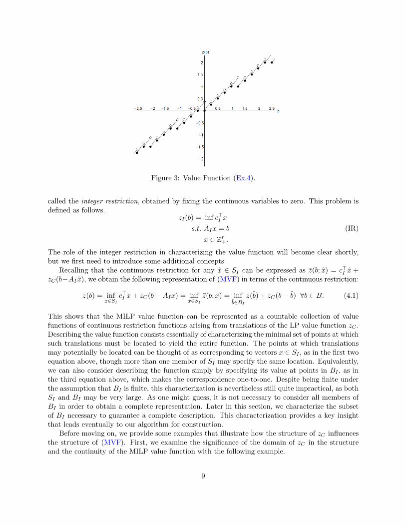
Figure 3: Value Function (Ex.4).
called the integer restriction, obtained by fixing the continuous variables to zero. This problem isdefined as follows.
zI(b) = inf c>I x
s.t. AIx = b
x ∈ Zr+.(IR)
The role of the integer restriction in characterizing the value function will become clear shortly,but we first need to introduce some additional concepts.
Recalling that the continuous restriction for any x ∈ SI can be expressed as z(b; x) = c>I x +zC(b−AI x), we obtain the following representation of (MVF) in terms of the continuous restriction:
z(b) = infx∈SI
c>I x+ zC(b−AIx) = infx∈SI
z(b;x) = infb∈BI
z(b) + zC(b− b) ∀b ∈ B. (4.1)
This shows that the MILP value function can be represented as a countable collection of valuefunctions of continuous restriction functions arising from translations of the LP value function zC .Describing the value function consists essentially of characterizing the minimal set of points at whichsuch translations must be located to yield the entire function. The points at which translationsmay potentially be located can be thought of as corresponding to vectors x ∈ SI , as in the first twoequation above, though more than one member of SI may specify the same location. Equivalently,we can also consider describing the function simply by specifying its value at points in BI , as inthe third equation above, which makes the correspondence one-to-one. Despite being finite underthe assumption that BI is finite, this characterization is nevertheless still quite impractical, as bothSI and BI may be very large. As one might guess, it is not necessary to consider all members ofBI in order to obtain a complete representation. Later in this section, we characterize the subsetof BI necessary to guarantee a complete description. This characterization provides a key insightthat leads eventually to our algorithm for construction.
Before moving on, we provide some examples that illustrate how the structure of zC influencesthe structure of (MVF). First, we examine the significance of the domain of zC in the structureand the continuity of the MILP value function with the following example.
9
Example 5. Consider again the value function (Ex.4). Its continuous restriction w.r.t x = 0 is
zC(b) = inf3
4x1 +
5
2x2
s.t.1
2x1 +
1
3x2 = b
x1, x2 ∈ R+.
Equivalently,
zC(b) = sup{νb : ν ≤ 3
2, ν ∈ R}. (4.2)
Here, the positive linear span of {12 ,13} is K = R+. We also have zC(b) = 3
2b for all b ∈ K. Thegradient of zC(b) at any b ∈ R+\{0} is 3
2 , which is the extreme point of the feasible region of (4.2).Note that for b ∈ R−, zC(b) = +∞ because the continuous restriction w.r.t the origin is infeasiblewhenever b ∈ R− and its corresponding dual problem is therefore unbounded. However, in themodification of this problem in (Ex.4), we have B = R, while K remains R+. This is because theadditional integer variables result in translations of K into R−. These translations result in thediscontinuity of the value function observed in (Ex.4).
The next result shows that the continuous restriction with respect to any fixed x ∈ SI bounds thevalue function from above, as it is a restriction of the value function by definition.
Proposition 4 For any x ∈ SI , z(·; x) bounds z from above.
Proof. For x ∈ SI we have
z(b; x) = c>I x+ zC(b−Ax) ≥ infx∈SI
c>I x+ zC(b−AIx) = z(b). 2
The second result shows that the continuous restriction with respect to the origin coincides withthe value function z over the intersection of K and some open ball centered at the origin. We denotean open ball with radius ε > 0 centered at a point d by Nε(d).
Proposition 5 There exists ε > 0 such that z(b) = zC(b) for all b ∈ Nε(0) ∩ K.
Proof. At the origin, we have z(0) = 0 with a corresponding optimal solution to the MILP being(x∗I , x
∗C) = (0, 0). For a given b ∈ R, as long as there exists an optimal solution x to the MILP with
right-hand side b such that x = 0, we must have z(b) = zC(b). Therefore, assume to the contrary.Then for every ε > 0, ∃b ∈ Nε(0) ∩ K, b 6= 0 such that zC(b) > z(b). Consider an arbitrary ε > 0and an arbitrary b ∈ Nε(0)∩K, b 6= 0 such that zC(b) > z(b). Then if x is a corresponding optimalsolution to the MILP with right-hand side b, we must have x 6= 0. Let E and E denote the set ofcolumn indices of sub-matrices of AC corresponding to optimal bases of the continuous restrictionsat 0 and x, respectively (note that both must exist).Case i. E = E. We have
zC(b) > z(b)⇒ c>EA−1E b > c>I x+ c>
EA−1Eb− c>
EA−1EAI x
⇒ 0 > c>I x− c>EA−1EAI x.
10

However, the last inequality implies that at the origin, (x, A−1EAI x) provides an improved solution
so that z(0) < 0, which is a contradiction.Case ii. AE 6= AE . We have zC(b) = c>EA
−1E b > c>
EA−1Eb, which is a contradiction of the fact that
zC is the value function of the continuous restriction at 0.
Example 6. Figure 4a shows that the epigraph of the value function of (Ex.1) coincides with the coneepi(zC) = cone{(2, 6), (−7, 7), (0, 1)} on N2.125(0). Similarly, Figure 4b demonstrates that the epi-graph of the discontinuous value function (Ex.4) coincides with epi(zC) = cone
{(12 ,
34), (13 ,
52), (0, 1)
}on N0.25(0) ∩ K = [0, 0.25) ⊆ R+.
(a) (b)
Figure 4: The MILP value function and the epigraph of the (CR) value function at the origin.
The characterization of the value function we proposed in (4.1) is finite as long as the set SI isfinite. However, there are cases where the set
BI = {b ∈ B : SI(b) 6= ∅}
is finite, while SI remains infinite. Clearly in such cases, there is a finite representation of the valuefunction that (4.1) does not provide. We can address this issue by representing the value functionin terms of the set BI rather than the set SI , but even then, the representation is not minimal,as not all members of BI are necessary to the description. We next study the properties of theminimal subset of BI that can fully characterize the value function of a MILP.
From the previous examples, we can observe that when the MILP has only a single constraintand the value function is thus piecewise linear, the points necessary to describe the function arethe lower break points. To generalize the notion of lower break points to higher dimension, we needsome additional machinery.
In Figure 4, the lower break points are also local minima of the MILP value function and onemay be tempted to conjecture that knowledge of the local minima is enough to characterize thevalue function. Unfortunately, it is easy to find cases for which the value function has no local
11
minima and yet still has the nonconvex structure characteristic of a general MILP value function.Consider the following example.
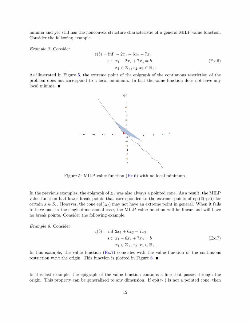
Example 7. Considerz(b) = inf − 2x1 + 6x2 − 7x3
s.t. x1 − 2x2 + 7x3 = b
x1 ∈ Z+, x2, x3 ∈ R+.
(Ex.6)
As illustrated in Figure 5, the extreme point of the epigraph of the continuous restriction of theproblem does not correspond to a local minimum. In fact the value function does not have anylocal minima.
Figure 5: MILP value function (Ex.6) with no local minimum.
In the previous examples, the epigraph of zC was also always a pointed cone. As a result, the MILPvalue function had lower break points that corresponded to the extreme points of epi(z(·;x)) forcertain x ∈ SI . However, the cone epi(zC) may not have an extreme point in general. When it failsto have one, in the single-dimensional case, the MILP value function will be linear and will haveno break points. Consider the following example.
Example 8. Considerz(b) = inf 2x1 + 6x2 − 7x3
s.t. x1 − 6x2 + 7x3 = b
x1 ∈ Z+, x2, x3 ∈ R+.
(Ex.7)
In this example, the value function (Ex.7) coincides with the value function of the continuousrestriction w.r.t the origin. This function is plotted in Figure 6.
In this last example, the epigraph of the value function contains a line that passes through theorigin. This property can be generalized to any dimension. If epi(zC) is not a pointed cone, then
12

Figure 6: Linear and convex MILP and CR value functions to (Ex.7).
for any given x ∈ SI , the boundary of the epigraph of z(·; x) contains a line that passes through(AI x, z(AI x; x)). The boundary of the resulting MILP value function therefore contains parallellines that result from translations of z. Clearly, to characterize such a value function, one wouldneed to have, for each such line, a point b such that (b, z(b)) is on both the line and the valuefunction of the continuous restriction, zC . This case, in which epi(zC) is not a pointed cone, is,however, an edge case and its consideration would complicate the presentation substantially. Forthe remainder of this section, we therefore assume the more common case in which epi(zC) is apointed cone.
To generalize the set of lower break points to higher dimension, we introduce the notion ofpoints of strict local convexity of the MILP value function. We denote the set of these points byBSLC .
Definition 1 A point b ∈ BI is a point of strict local convexity of the function f : Rm → R∪{±∞}if for some ε > 0 and g ∈ Rm, we have
f(b) > f(b) + g>(b− b) for all b ∈ Nε(b), b 6= b.
This definition requires the existence of a hyperplane that is tangent to the function f at the pointb ∈ BI , while lying strictly below f in some neighborhood of b. For the continuous restrictionwith respect to x ∈ SI , this can happen only at the extreme point of the epigraph of the function,if such a point exists. Note that at such a point, we must have z(b; x) = c>I x. Furthermore, if
x ∈ arg infx∈SIz(b;x), then we will also have z(b; x) = zI(b).
Proposition 6 For a given x ∈ SI , b ∈ AI x+K is a point of strict local convexity of z(·; x) if andonly if (b, z(b; x)) is the extreme point of epi(z(·; x)).
Proof. Let x ∈ SI and b ∈ AI x + K be given as in the statement of the theorem. We use thefollowing property in the proof. Let the function Ht be defined by
Ht(b) =
{c>I x+ (b−AI x)>ηt for b ∈ K,+∞ otherwise,
13

where ηt ∈ {νi}i∈K ∪ {dj}j∈L. Then, we have
z(b; x) = supt∈K∪L
Ht(b)
Moreover,∂z(b; x) = conv({∇H1, . . . ,∇Hp}p∈P ) = conv({η1, . . . , ηp}p∈P ) 6= ∅,
where P ⊆ K ∪ L and |P | > 1 and finally, we have that
z(b; x) = H1(b) = · · · = Hp(b) for p ∈ P. (4.3)
(⇒) Let ε and g be the radius of the ball and a corresponding subgradient showing the strict localconvexity of z(·; x) at b. If z(·; x) is differentiable at b, then ∃ν ∈ Rm such that ∂z(·; x) = {ν}, andtherefore g = ν. Then we trivially have that b cannot be a point of strict local convexity of z(·; x),as there always exists ε′ with 0 < ε′ < ε such that on Nε′(b), we have z(b; x) = z(b; x) + ν>(b− b).Therefore, z(·; x) cannot be differentiable at b.
Since z(·; x) is not differentiable at b, there are H1, . . . ,Hp, p ∈ P , as defined above. In the case
that p > m, from the discussion in Section 3, b has to be the extreme point of epi(z(·; x)). Next,we show that b cannot be the extreme point of epi(z(·; x)) if p ≤ m.
When 1 < p ≤ m, equation (4.3) must still hold. Let
R = {(b, z(b; x)) ∈ (AI x+K)× R : z(b; x) = H1(b) = · · · = Hp(b) for p ∈ P}
Then there exists b ∈ Nε(b) such that (b, z(b)) ∈ R and b 6= b. We have
z(b; x)− z(b; x) = (b− b)>ηt, t ∈ P.
Then we can conclude that for g ∈ ∂z(b; x) = conv({η1, . . . , ηp}), the function z(b; x)+g>(b− b) alsocoincides with z(b; x) as follows. Choose 0 ≤ λt ≤ 1, t ∈ P such that g =
∑t∈P λ
tηt,∑
t∈P λt = 1.
From the equationsλt(z(b; x)− z(b; x)) = λt(b− b)>ηt, t ∈ P
we have a contradiction to b being the point of strict local convexity of z(·; x), since
z(b; x)− z(b; x) =
p∑t=1
λt(b− b)>ηt = g>(b− b).
(⇐) Since (b, z(b)) is the extreme point of epi(z(·; x)), then ∂z(b; x) = conv({η1, . . . , ηp}), wherep ∈ P and we must have that |P | > m. Choose g ∈ int(conv({η1, . . . , ηp})). For an arbitraryb ∈ AI x + K, b 6= b there exists η ∈ {η1, . . . , ηp} such that z(b; x) = (b − AI x)>η. Then, from themonotonicity of the subgradient of a convex function we have (η> − g>)(b− b) > 0. Therefore,
z(b; x) = z(b; x) + η>(b− b) > z(b; x) + g>(b− b) ∀b ∈ AI x+K, b 6= b. (4.4)
That is, b is a point of strict local convexity of z(·; x).
Example 9. Consider the MILP in Example 4. The blue shaded region in Figure 7 is epi(z(·; 1)).The point (1,−2) is the extreme point of the cone epi(z(b; 1)) and b = 1 is a point of strict localconvexity of the value function.
Next, we discuss the points of strict local convexity of the MILP value function.
14

Figure 7: The value function of the MILP in (Ex.6)
Proposition 7 If b is a point of strict local convexity, then there exists x ∈ SI such that
• b = AI x;
• (b, z(b; x)) is the extreme point of epi(z(·; x)); and
• z(b; x) = c>I x = zI(b) = z(b).
Proof. Let b be a point of strict local convexity. If there exists x ∈ SI(b) such that x ∈arg infx∈SI
z(b;x), then we have that c>I x = z(b). The remainder of the statement is trivial in
this case. Consider the case where such x does not exist. That is, for any (x, y) ∈ S(b) such thatc>I x+ c>Cy = z(b), we have y > 0. Let one such point be (x, y). Consider ε > 0 used to show b is a
point of strict local convexity. If z(·; x) coincides with z on Nε(b), then from from Proposition 6 itfollows that b cannot be a point of strict local convexity. On the other hand, if z is constructed bymultiple translations of z over Nε(b), since it attains the minimum of these functions, there cannotbe a supporting hyperplane to z at b, therefore b cannot be a point of strict local convexity.
We note that the reverse direction of Proposition 7 does not hold. In particular, it is possiblethat for some x ∈ SI we have z(AI x) = c>I x, but that AI x is not a point of strict local convexity.For instance, in example 1, for x = (1, 0, 1) we have that AI x = 2 and that z(2; x) = z(2) = 6.Nevertheless, 2 is not a point of strict local convexity.
Points of strict local convexity may lie on the boundary of BI . The next example illustrates acase where this happens.
Example 10. Consider the MILP value function
z(b) = inf − x1 + 3x2
s.t. x1 − 3x2 = b
x1 ∈ Z+, x2 ∈ R+.
(Ex.9)
shown in Figure 8. If we artificially impose the additional restriction that b ∈ [0, 2] for the purposes
15

Figure 8: MILP Value Function of (Ex.9) with BI = [0, 2].
of illustration, it is clear that there is no point of strict local convexity in the interior of BI , althoughepi(zC) is a pointed cone.
Let us further examine the phenomena illustrated by the previous example. For a given x ∈ SI , letb = AI x. We know that the single extreme point of epi(z(·; x)) is (b, z(b; x)) and that there musttherefore be m+ 1 (2 in this example) facets of epi(z(·; x)) whose intersection is this single extremepoint. Now, if b is not a point of strict local convexity, then on any Nε(b) with ε > 0, at most mfacets of epi(z(·; x)) coincide with the facets of the epigraph of the value function. This means thatthere exists a direction in which z is affine in the neighborhood of (b, z(b; x)); that is, b cannot bea point of strict local convexity of z. Given that the set BI is assumed to be bounded, the valuefunction must contain a point (b, z(b)) such that b ∈ bd(conv(BI))∩BI along a line in this direction.Let bd(BI) = bd(conv(BI)) ∩ BI . Since epi(zC) is pointed, then b has to be a point of strict localconvexity of z. This latter point is the one needed to describe the value function—the epigraph ofthe associated continuous restriction associated with b contains the continuous restriction w.r.t. x,which means that Ax is not contained in the minimal set of points at which we need to know thevalue function.
We are now almost ready to formally state our main result. So far, we have discussed certainproperties of the points of strict local convexity and showed that such points can belong to theinterior or boundary of BI . Our goal is to show that the set BSLC , which was previously definedto the set of all points of strict local convexity, is precisely the minimal subset of BI , denoted inthe following result by Bmin, needed to characterize the full value function. Let us now formallydefine Bmin to be a minimal subset of BI such that
z(b) = infb∈Bmin
z(b) + zC(b− b) ∀b ∈ B. (4.5)
Then we have the following result.
Proposition 8 Bmin = BSLC .
Proof. First, we show that if b ∈ B\BSLC , then it is not in the set Bmin. If b ∈ B\BI , thenfrom (4.1) it follows that b is not necessary to describe the value function, then b /∈ Bmin. Consider
16

b ∈ BI\BSLC . Let x ∈ SI(b) such that c>I x = z(b). Since epi(zC) is assumed to be pointed, we
have z(b) = min{z(b;x1), z(b;x2),. . . , z(b;xk)}, where k > 1 and x1, . . . , xk ∈ SI . Then, for some l = 1, . . . , k and xl 6= x we havemin{z(b; x), z(b;xl)} = z(b;xl) and it follows that b /∈ Bmin. Therefore, if b ∈ Bmin, then b ∈ BSLC .
We next show that if b ∈ BSLC , then b ∈ Bmin. Let us denote by S′(b) the set of points x ∈ SIsuch that (AIx, c
>I x) coincides with the value function at b. If b /∈ Bmin, then all the points in S′(b)
can be eliminated from the description of the value function in (4.1). That is, we have
z(b) = infx∈SI\S′(b)
z(b;x).
Therefore, for any pair (x, y) ∈ S(b) that is an optimal solution to the MILP with right-hand sidefixed at b, we have y > 0. This, however, contradicts with Proposition 7 and we have that b cannotbe a point of strict local convexity of z.
Because it will be convenient to think of the value function as being described by a subset of SI ,rather than as a subset of BI , we now express our main result in those terms. From Proposition 8,it follows that there is a subset of Smin of SI that can be used to represent the value function, asshown in the following theorem. Note, however, that while Bmin is unique, Smin is not.
Theorem 1 (Discrete Representation) Let Smin be any minimal subset of SI such that for anyb ∈ Bmin, ∃x ∈ Smin such that AIx = b and c>I x = z(b).Then for b ∈ B, we have
z(b) = infx∈SI
z(b;x) = infx∈Smin
z(b;x). (4.6)
Proof. The proof follows from Proposition 8, noting that a point x ∈ SI such that c>I x > z(AIx)cannot be necessary to describe the value function.
Example 11. We apply the theorem to (Ex.1). In this example, over b ∈ [−9, 9], we have thatBmin = {−8,−4, 0, 5, 6, 10} and Smin = {[0; 0; 2], [0; 0; 1], [0; 0; 0], [0; 1; 0], [1; 0; 0], [0; 2; 0]}. Clearly,the knowledge of the latter set is enough to represent the value function.
Theorem 1 provides a minimal subset of SI required to describe the value function. We discussin Section 7 that constructing a minimal such subset exactly may be difficult. Alternatively, wepropose an algorithm to approximate Smin (with a superset that is thus still guaranteed to yieldthe full value function). This has proven empirically to be a close approximation. Before furtheraddressing the practical matter of how to generate the representation, we discuss some theoreticalproperties of the value function that arise from our result so far in the next two sections. Thereader interested in the computational aspects of constructing the value function can safely skipto Section 7 for the proposed algorithm, as that algorithm does not depend on the results in thefollowing two sections.
17

5 Local Stability Regions
In this section, we demonstrate that certain structural properties of the value function, such asregions of convexity and points of non-differentiability and discontinuity, can also be characterizedin the context of our representation. We show that there is a one-to-one correspondence betweenregions over which the value function is convex and continuous—the so-called local stability sets—and the set Bmin. We also provide results on the relationships between this set and the sets ofnon-differentiability and discontinuity of the value function.
We start this section by introducing notation for the sets of right-hand sides with particularproperties.
Definition 2
• BLS(b) = {b ∈ B : z(b) = z(b) + zC(b− b)} is the local stability set w.r.t b ∈ B;
• BES(b) = bd(BLS(b)) is the local boundary set w.r.t b ∈ B;
• BES = ∪b∈BminBES(b) is the boundary set;
• BND = {b ∈ B : z is not differentiable at b} is the non-differentiability set; and
• BDC = {b ∈ B : z is discontinuous at b} is the discontinuity set.
Example 12. To illustrate the above definitions, consider the value function in Example 1. Letb = 3. Over the interval [−9, 9] we have that the function z(3) + zC(b − 3) coincides with z atb ∈ BLS(b) = [2.125, 3]. Then, BES(b) = {2.125, 3}. The minimal set is Bmin = {−8,−4, 0, 5, 6}.The boundary set consists of the union of the local boundary sets w.r.t. minimal points; i.e.,
BES ={{−9,−7.75} ∪ {−7.75,−3.75} ∪ {−3.75, 2.125} ∪ {2, 125, 5.125} ∪ {5.125, 8}}={−9,−7.75,−3.75, 2.125, 5.125, 8}.
The non-differentiablity set is
BND = {−9,−8,−7.75,−4,−3.75, 0, 2.125, 5, 5.125, 6, 8, 9}.
Finally, BDC = ∅.
The main result of this section is Theorem 2. The goal is to show that the value function is convexand continuous over the the local stability sets associated with the members of Bmin. Furthermore,in this theorem we demonstrate the relationship between the set Bmin, the boundary set, BES , andthe sets of point of non-differentiability and discontinuity of the value function. We next state thetheorem.
Theorem 2
i. Let b ∈ B.
– There exists x∗ ∈ Smin such that for any b ∈ int(BLS(b)), there exists y ∈ Rn−r+ such
that (x∗, y) is an optimal solution to the MILP with right-hand side b.
18

– z is continuous and convex over int(BLS(b)).
ii. b ∈ BES if and only if for any ε > 0, @x∗ ∈ SI such that z(b) = c>I x∗ + zC(b− AIx∗) for all
b ∈ Nε(b).
iii. Let b ∈ Bmin. Then, int(BLS(b)) is the maximal set of right-hand sides containing b overwhich the value function is convex and continuous.
iv. For the general MILP value function, we have Bmin ⊆ BND and BES ⊆ BND. Furthermore,if the MILP value function is discontinuous, we have Bmin ⊆ BDC ⊆ BES ⊆ BND.
Proof. We build to the proof of the theorem, which constitute the remainder of this section, byproving lemmas 1–8, The first and second parts of the theorem follow from lemma 1 and lemma 2.The third part of the theorem is shown in lemma 3. The last part follows from lemmas 5–8.
In the first lemma, we show properties of the function on differentiable regions within local stabilitysets.
Lemma 1 Let b ∈ B. Then there exists x∗ ∈ SI such that for any b ∈ int(BLS(b)), there existsy ∈ Rn−r+ such that (x∗, y) is an optimal solution to the MILP with right-hand side b. Furthermore,
z is continuous and convex over int(BLS(b))
Proof. From Theorem 1, for any b ∈ B there exists x∗ ∈ Smin such that int(BLS(b)) = int({b ∈B : z(b) = c>I x
∗ + zC(b − AIx∗)}). Therefore, for any b ∈ int(BLS(b)), z(b) = c>I x∗ + c>Cy
∗ where
y∗ = argmin{c>Cy : ACy = b− AIx∗, y ∈ Rn−r+ }. The convexity and continuity of z on int(BLS(b))follows trivially.
Corollary 1 If z is differentiable over N ⊆ B, then there exist x∗ ∈ SI and E ∈ E such thatz(b) = c>I x
∗ + ν>E (b−AIx∗) for all b ∈ N .
Proof. Let an arbitrary b ∈ N be given. By Theorem 1, we know that there exists x∗ ∈ Sminsuch that z(b) = z(b; x) and AIx
∗ ∈ Bmin. Then, we have z(b) = c>I x∗ + ν>E (b−AIx∗) with E ∈ E
and there exists (x∗, xE , xN ), an optimal solution to the given MILP with right-hand side b, wherexE and xN correspond to the basic and non-basic variables in the corresponding solution to thecontinuous restriction w.r.t. x∗. It follows that the vector (x∗, xE + A−1E (b − b), xN ) is a feasiblesolution for any b ∈ N .
Now, let another arbitrary point b ∈ N be given. We show that (x∗, xE +A−1E (b− b), xN ) must
be an optimal solution for right-hand side b. Since b ∈ N , b ∈ N and z is differentiable over N ,then νE is the unique optimal dual solution to the continuous restriction by Proposition 2 and wehave
z(b) = c>I x∗ + c>E(xE +A−1E (b− b)) + c>NxN
= z(b) + ν>E (b− b) = c>I x∗ + ν>E (b−AIx∗) + ν>E (b− b)
= c>I x∗ + ν>E (b−AIx∗) = z(b;x∗).
19

Since b and b were arbitrary points in N , the result holds for all such pairs and this ends the proof.
It follows from the previous result that if the value function is differentiable over N ⊆ B, thenits gradient at every right-hand side in N is a unique optimal dual solution to the continuousrestriction problem w.r.t. some x∗ ∈ SI . This generalizes Proposition 2 on the gradient of the func-tion at a differentiable point of the LP value function to the mixed integer case. As an example,in (Ex.4) the gradient of z at any differentiable point is ν = 3
2 . Next, we show the second part ofTheorem 2 in the following result.
Lemma 2 b ∈ BES if and only if for any ε > 0, @x∗ ∈ SI such that z(b) = c>I x∗ + zC(b − AIx∗)
for all b ∈ Nε(b).
Proof. (⇒) Let ε > 0 be given and assume ∃x∗ ∈ SI such that z(b) = c>I x∗ + zC(b − AIx
∗)
for all b ∈ Nε(b). Now, let b ∈ Bmin be such that b ∈ BES(b). Then for all b ∈ Nε(b), we havez(b) = z(b;x∗) = z(b) + zC(b− b). That is, b ∈ int(BLS(b)).
(⇐) Let b ∈ Bmin be such that b ∈ int(BLS(b)). Then from Lemma 1, there exists x∗ ∈ SIoptimal for all b ∈ BLS(b).
Next, we arrive at showing the third part of Theorem 2. This is shown in the following result.
Lemma 3 Let b ∈ Bmin. Then, int(BLS(b)) is the maximal set of right-hand sides containing bover which the value function is convex and continuous.
Proof. Assume the contrary that BLS(b) with b ∈ Bmin is not the maximal set. Then, there existsb in the boundary set w.r.t b, BES(b), and ε > 0 such that the value function is continuous andconvex at Nε(b). From Theorem 1 and Lemma 2 we have
z(b) = minxi∈Smin
{c>I xi + (b−AIxi)>νi}, b ∈ Nε(b), (5.1)
where νi is the optimal dual solution to zC(b− AIxi) and the set xi ∈ Smin contains two or moredistinct members. Then, z is concave over Nε(b) unless all the polyhedral functions in (5.1) are thesame. But then Nε(b) is a subset of BLS(b).
So far, in Theorem 2 we have demonstrated that over the local stability set w.r.t a minimal point,the integer part of the solution to the MILP remains constant and the value function of the MILPis a translation of the continuous restriction value function. This can be viewed as a generalizationof a similar result that the value function of a PILP with inequality constraints is constant over itslocal stability sets (zC(b) = 0 for b ∈ Rm). These regions are characterized by Schultz et al. (1998).In this case, the members of Bmin generalize the notion of minimal tenders discussed in (Trappet al., 2013).
Before showing the forth and last part of Theorem 2, we need another lemma on the necessaryconditions for the continuity of the value function.
Lemma 4 If zC(b) <∞ for all b ∈ B, then z is continuous over B.
20

Proof. If zC(b) < ∞ for some b ∈ B, then the continuous restriction w.r.t. the origin and itsdual are both feasible and have optimal solution values equal to zC(b). Therefore, z is finite andcontinuous on B. It can be proved by induction that the minimum of countably many continu-ous functions defined on B is continuous on B. The continuity of z follows by the representationin (4.1).
We now proceed to show the last part of the theorem. Lemmas 5–8 address the relationshipsbetween the discontinuity set of the value function with the minimal set of right-hand sides, theboundary set, and the set of non-differentiability points. Combining the following lemmas, theproof of the theorem is complete.
Lemma 5 Bmin ⊆ BND.
Proof. Assume the value function is differentiable at some b ∈ Bmin. Let ∇z(b) = g. Then, thereexists some ε > 0, such that z(b) = z(b) + g>(b− b) for all b ∈ Nε(b). But then, from the definitionof a point of strict local convexity, b cannot be in BSLC and therefore, b /∈ Bmin.
Earlier we showed that the discontinuities of the MILP value function may only happen whenit no longer attains its minimum over some translated z and a switch to another translation isrequired. This is used next to show the relationship between the discontinuity and boundary sets.
Lemma 6 BDC ⊆ BES.
Proof. Assume to the contrary that there exists b ∈ BDC but b ∈ int(BLS(b)) for some b ∈ Bmin.Then from Theorem 2, there exists ε > 0 such that z(b) = z(b) + zC(b − b) for all b ∈ Nε(b).Therefore, z can only be continuous on Nε(b), which is a contradiction.
Lemma 7 If the value function is discontinuous, then Bmin ⊆ BDC .
Proof. Since BDC 6= ∅, from Lemma 4 we have K 6= Rm. Then, for any b ∈ B we have b ∈ BES(b);that is, any right-hand side lies on the boundary of its local stability set. Consider b ∈ Bmin. If z iscontinuous at b then there exists ε > 0 and b ∈ Bmin such that b 6= b and for any b1 ∈ Nε(b)\BES(b)we have z(b1) = z(b) + zC(b1 − b). Consider b2 ∈ Nε(b)∩BES(b). If z(b) + zC(b2 − b) < z(b2), thenz cannot be the value function at b2. On the other hand, if z(b) + zC(b2− b) lies above or on z(b2),it can be easily shown that there cannot exist a supporting hyperplane of z at b that lies strictlybelow z on an arbitrarily small neighborhood of b. Then b cannot be in Bmin.
The next result shows that if b belongs to the boundary set w.r.t a minimal point, then z isnon-differentiable at b.
Lemma 8 BES ⊆ BND.
Proof. Assume there exist some b ∈ BES(b), b ∈ Bmin such that z is differentiable at b. Thenthere exists ε > 0 and E ∈ E such that for all b ∈ Nε(b) we have
z(b) = z(b) + ν>E (b− b)= z(b) + ν>E (b− b) + ν>E (b− b)= z(b) + ν>E (b− b) = z(b) + zC(b− b).
(5.2)
21

Figure 9: Local stability sets and corresponding integer part of solution in (Ex.1).
But this contradicts the third part of Theorem 2.
We finish this section by applying Theorem 2 to the continuous value function in Example 1and the discontinuous value function in Example 4.
Example 13. Consider the value function (Ex.1). Figure 9 shows the optimal integer parts x1, . . . , x4
of solutions to the corresponding MILP over the local stability sets BLS(−4), BLS(0), BLS(5) andBLS(6), respectively. One can observe that both the minimal set and the boundary set of the valuefunction are subsets of its set of non-differentiability points.
Similarly, in Example 4, x1 = [1 2]>, x2 = [2 3]>, x3 = [3 4]>, x4 = [0 0]>, x5 = [1 1]>, x6 =[2 2]>, x7 = [3 3]> are respectively the integer parts of the solutions for right-hand sides in the localstability sets BLS(−0.75), BLS(−0.5), . . . , BLS(0.5), BLS(0.75). In this case, the value function isdiscontinuous on the points that belong to the minimal set and we have Bmin ∪ BES = BES =BDC = BND.
Remark 1 If z is continuous over B, then SD 6= ∅. This follows from the fact that if SD = ∅,then z(0) = zC(0) = −∞ which contradicts z(0) = 0. Therefore, we have that zC(b) > −∞ for allb ∈ Rm. However, we may still have zC(b) =∞ for some b ∈ Rm. The following is an example.
Example 14. The value function defined by (Ex.12) below is continuous on R, although K = R+.
z(b) = inf x1 − x2s.t. − x1 + x2 = b
x1 ∈ Z+, x2 ∈ R+.
(Ex.12)
22

6 A Simplified Jeroslow Formula
The representation we have just described is related (though not so obviously) to a closed formrepresentation of the MILP value function identified by Blair (1995), which he called the JeroslowFormula. In this formula, the value function is obtained by taking the minimum of |E| functions,each consisting of a PILP value function and a linear term. In this section, we study the connectionbetween our representation of the MILP value function and the representation in the JeroslowFormula and provide a simpler representation of it.
Let us denote by b·c the component-wise floor function. For E ∈ E , we define
bbcE = AE⌊A−1E b
⌋∀b ∈ B, TE = {b ∈ B : A−1E b ∈ Zm}, and T =
⋂E∈E
TE .
Consider a given b ∈ K. Let E ∈ E be such that xE = A−1E b is the corresponding solution to the
continuous restriction w.r.t. the origin. If b ∈ TE , it follows that b = AE xE is an integer linearcombination of vectors in feasible basis AE . Hence, the same is true for any member of T .
Now consider the continuous restriction w.r.t to a given x ∈ SI . Then we have more generallythat the corresponding solution to the continuous restriction w.r.t. x at a given b ∈ K +AI x is
xE = A−1E (b−AI x),
where E ∈ E . In this case, when b ∈ T , we can no longer guarantee that xE ∈ Zm. By anappropriate scaling, however, we can ensure this property, and this is one of the key steps inderiving the Jeroslow formula. Since all matrices are assumed to be rational, there exists M ∈ Z+
such that MA−1E Aj ∈ Zm for all E ∈ E and all j ∈ I, with Aj denoting the jth column of A. Then,since A−1E b is integral for any b ∈ T and E ∈ E , we have that the value function of the followingPILP is equal to the value function of the original MILP for all b ∈ T .
Proposition 9 (Blair, 1995) There exists M ∈ Z+ such that z(b) = zM (b) for all b ∈ T , where
zM (b) = inf c>I x+1
Mc>Cy
s.t. AIx+1
MACy = b
(x, y) ∈ Zr+ × Zn−r+ .
(6.1)
Proof. Let M ∈ Z+ such that MA−1E Aj is a vector of integers for all E ∈ E and j ∈ I. Scaling ACand cC by 1
M in (MVF) guarantees that Aj ∈ T for all j ∈ I. Therefore, MA−1E (b−AIx) ∈ Zm forall x ∈ Zr and E ∈ E . It follows that the solution value to z and zM is equal for any b ∈ T .
We illustrate the scaling procedure in the following example.
Example 15. Consider Example 1. In (Ex.1) we have AjI ∈ {6, 5,−4} for j = 1, . . . , 3 and E =
23

{{1}, {2}} with A{1} = 2 and A{2} = −7. We choose M = 14 so that MA−1E AjI ∈ Z for all E ∈ E .The corresponding scaled PILP problem is
zM (b) = inf 3x1 +7
2x2 + 3x3 +
3
7x4 +
1
2x5
s.t. 6x1 + 5x2 − 4x3 +1
7x4 −
1
2x5 = b
x1, x2, x3, x4, x5 ∈ Z+.
(6.2)
Figure 10a demonstrates the value function (6.2) for b ∈ [−9, 9]. From the figure we can see thatz and zM coincide on intervals of length 1
7 where A{1} = 2 is optimal, while the two functions
coincide at intervals of length 12 where A{2} = −7 is optimal.
Let us have a closer look at the interval [2, 2.6] illustrated in Figure 10b. The set of feasibleright-hand sides for the scaled PILP (6.2) in this interval is {2, 2 1
14 , 2214 , 2
314 , , . . . , 2
814}. Among
these points, the value function coincides with (6.2) at 2 and 2.5. We have
z(b) = zC(b) = ν{1}b = 3b, for b ∈ [2, 2.125]
and
z(b) = z(b; [0, 1, 0]>) =7
2+ ν{2}(b− 5) =
7
2− (b− 5), for b ∈ [2.125, 2.6].
Since T{1} = {b : MA−1{1}b = 7b ∈ Z}, we have T{1} ∩ [2, 2.6] = {b : b = i7 , i = 14, . . . , 18}. Similarly,
T{2} ∩ [2, 2.6] = {b : b = i2 , i = 4, 5}.
(a) (b)
Figure 10: The scaled PILP value function (6.2).
Over the intervals for which AE∗ is the optimal dual basis for the corresponding continuousrestriction, z and zM coincide at TE∗ = {b ∈ B : b = bbcE∗ = kMA−1E∗ , k ∈ Z+}. For instance,z(2) = zM (2) with 2 ∈ T{1}, but z(21
7) 6= zM (217) with 21
7 ∈ T{1}. This is due to the fact that A{1}is the optimal dual basis at z(2) = zC(2) but not at z(21
7 ; [0, 1, 0]>) = z(217).
Remark 2 Note that the z and zM may coincide at some right-hand side that is not in the set T ,e.g., b = 2.5 ∈ T{2}\T{1}.
24

Blair and Jeroslow (1984) identified a class of functions called Gomory functions and showedthat for any PILP, there exists a Gomory function whose value coincides with that of the valuefunction of the PILP wherever it is finite. To extend this result to the MILP case, Blair (1995)proposed “rounding” any b ∈ B to some bbcE with E ∈ E and evaluating the latter using a PILP.Note that (6.1) has to be modified to be used for this purpose, since it is not necessarily feasiblefor all bbcE , E ∈ E ; i.e., it is possible to have xE = M(A−1E −A
−1E AI x) < 0 for x ∈ Zr+. To achieve
feasibility for all bbcE , Blair (1995) proposed the following modification of (6.1) and used it in theJeroslow formula.
zJF (t) = inf c>I x+1
Mc>Cy + z(− 1
M
∑j∈C
Aj)y
s.t. AIx+1
MACy + (− 1
M
∑j∈C
Aj)y = t
y ∈ Zn−r+ , x ∈ Zr+, y ∈ Z+.
(6.3)
Finally, he used linear terms of the form of ν>E (b − bbcE) to compensate for the “rounding” ofb to bbcE with E ∈ E . Together, he showed that for any MILP, there is a Gomory function Gcorresponding to the value function of the PILP (6.3) with
z(b) = infE∈E{G(bbcE) + ν>E (b− bbcE)}. (6.4)
The representation of the value function in (6.4) is known as the Jeroslow Formula.Although it is a bit difficult to tease out, given the technical nature of the Jeroslow Formula,
there is an underlying connection between it and our representation. In particular, the set T has arole similar to the role of Bmin in our representation—it is a discrete subset of the domain of thevalue function of the original MILP over which the original value function agrees with the valuefunction of a related PILP. This is the same property our set Bmin has and it is what allows thevalue function to have a discrete representation. Furthermore, the correction terms in the JeroslowFormula play a role similar to the value function of the continuous restriction in our representation.
The advantage our representation has over the Jeroslow Formula is that Bmin is potentially amuch smaller set and the value M in the Jeroslow formula would be difficult to calculate a priori.Furthermore, even if M could be obtained in some cases, evaluating the value function for a givenb ∈ B using the Jeroslow formula ostensibly requires the evaluation of a Gomory function for everybbcE for all E ∈ E , including those feasible bases AE that are not optimal at b. The number ofevaluations required is equal to the size of
⋃E∈E TE . These drawbacks relegate the Jeroslow formula
to purely theoretical purposes. On the surface, there does not seem to be any way to utilize it inpractice. Nevertheless, it is possible to simplify the Jeroslow Formula, replacing T by Bmin andeliminating the need to calculate M in the process. This leads to a more practicable variant of theoriginal formula. First, we show formally that Bmin is a subset of T .
Proposition 10 Bmin ⊆ T .
Proof. Let (x, y) be an optimal solution to (MVF) at b ∈ Bmin. From Proposition 7, we have thaty = 0 in any optimal solution of the value function at b. Then for all E ∈ E we have⌊
b⌋E
=1
MAE⌊MA−1E AI x+MA−1E AC y
⌋= AI x = b.
25

Then,⌊b⌋E
= b for all E ∈ E and b ∈ T .
Corollary 2 If b ∈ Bmin, then z(b) = zI(b) = zM (b) = zJF (b) = G(b) where G is the PILP valuefunction in (6.4).
Proof. The first equality follows from Proposition 7. The second equality holds since y = 0 inany optimal solution to (MVF) at a right-hand side in Bmin. zM (b) is equal to zJF (b) since forb = bbcE for all b when b ∈ Bmin and y can be fixed to zero in (6.3). The last equality holds forany bbcE , E ∈ E .
Theorem 3 (Simplified Jeroslow formula)
z(b) = infb∈Bmin,E∈E
{zI(b)− ν>E (b− b)}. (6.5)
Proof. We havez(b) = inf
E∈E{G(bbcE) + ν>E (b− bbcE)}
= infb∈TE ,E∈E
{G(b) + ν>E (b− b)}
= infb∈Bmin
{zI(b) + supE∈E
ν>E (b− b)}
= infb∈Bmin,E∈E
{zI(b)− ν>E (b− b)}.
The first equation is the Jeroslow Formula. The second one is because bbcE ∈ TE for any E ∈ Eand b ∈ B. From Theorem 1, z(b) = inf{z(b;x) : AIx ∈ Bmin}, then the third equality holds. Thelast equation follows trivially.
The above result provides a variation of the Jeroslow formula where there is no need to find thevalue of M , or to evaluate the PILP value function zJF for members of
⋃E∈E TE . Instead, we need
to evaluate the simpler PILP value function zI for the set Bmin ⊆ T ⊆⋃E∈E TE . The difference in
the size of Bmin and⋃E∈E TE can be significant. We provide an illustrative example next.
Example 16. The value function of (6.2) for right-hand sides in T{1} ∪ T{2} is plotted in Figure 11
with filled blue circles. At a point b ∈ T{1} ∪ T{2}, we have zM (b) = G(b) where G is the Gomoryfunction corresponding to the PILP (6.2). The Jeroslow formula for the MILP value functionover [−9, 9] requires finding all such points. Alternatively, we can have a smaller representation byconstructing the value function of the integer restriction of (Ex.1). i.e., zI(b) = inf{3x1+ 7
2x2+3x3 :
6x1 + 5x2 − 4x3 = b, x1, x2, x3 ∈ Z+}. This value function is plotted in Figure 12. However, thealternative formulation (6.5) requires finding G(b) = zI(b) for b ∈ Bmin = {−8,−4, 0, 4, 5, 10}.
26

Figure 11: The value function of (6.2) for b ∈ T{1} ∪ T{2} ∪ [−9, 9].
7 Finite Algorithm for Construction
In this final section, we discuss the use of our representation in computational practice, which isthe ultimate goal of this work. To sum up what we have seen so far, we have shown that thereexists a discrete set Smin (not necessarily unique) over which the value of z can be determined bysolving instances of the integer restriction. Theorem 1 tells us that, in principle, if we knew z(AIx)for all x ∈ Smin, then z(b) could be computed at any b ∈ B by solving |Smin| LPs.
Our discrete representation of the value function in Theorem 1 is equivalent to
z(b) = infx∈Smin
c>I x+ zC(b−AIx). (7.1)
If |Smin| is relatively small, this yields a practical representation. The most straightforward way toutilize our representation would then be to generate the set Smin a priori and to apply the aboveformula to evaluate z(b) for b 6∈ Bmin.
In general, obtaining an exact description of the set Smin seems to be difficult. One solutionto this problem would be to instead generate the value function of the integer restriction first bythe procedure of Kong et al. (2006), which is finite under our assumptions. We illustrate thishypothetical procedure in the following example.
Example 17. Consider constructing the value function defined by (Ex.1) for b ∈ [−7, 7]. The valuefunction of the integer restriction zI is plotted in Figure 12. Clearly, complete knowledge of zI isunnecessary to describe the MILP value function, as this requires evaluation for each point in SI ,whereas we have already shown that evaluation of points in Smin is enough. In this example, overb ∈ [−7, 7], we have that Smin = {0; 0; 1], [0; 0; 0], [0; 1; 0], [1; 0; 0]}. Therefore, four evaluations isenough, yet at least 15 are required for constructing the value function of the PILP.
Hence, this approach does not seem to be efficient. Instead, we anticipate overcoming this difficultyin two different ways, depending on the context in which the value function is needed. First,working with a subset of Smin still yields an upper approximation of z, which might be useful
27
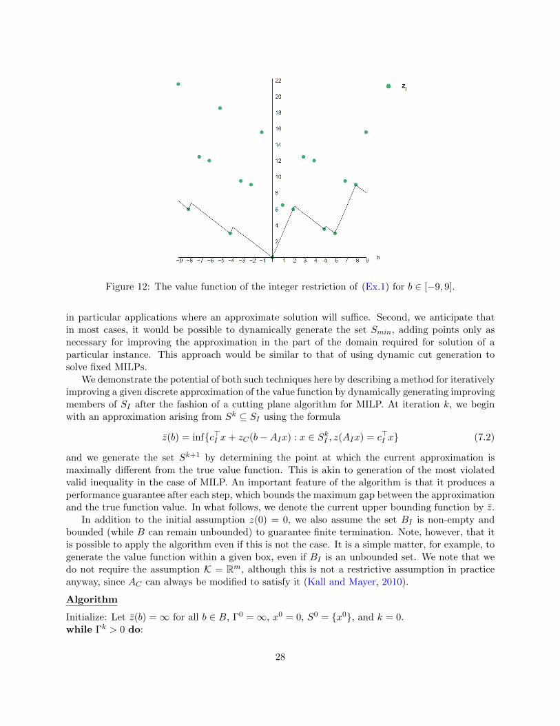
Figure 12: The value function of the integer restriction of (Ex.1) for b ∈ [−9, 9].
in particular applications where an approximate solution will suffice. Second, we anticipate thatin most cases, it would be possible to dynamically generate the set Smin, adding points only asnecessary for improving the approximation in the part of the domain required for solution of aparticular instance. This approach would be similar to that of using dynamic cut generation tosolve fixed MILPs.
We demonstrate the potential of both such techniques here by describing a method for iterativelyimproving a given discrete approximation of the value function by dynamically generating improvingmembers of SI after the fashion of a cutting plane algorithm for MILP. At iteration k, we beginwith an approximation arising from Sk ⊆ SI using the formula
z(b) = inf{c>I x+ zC(b−AIx) : x ∈ SkI , z(AIx) = c>I x} (7.2)
and we generate the set Sk+1 by determining the point at which the current approximation ismaximally different from the true value function. This is akin to generation of the most violatedvalid inequality in the case of MILP. An important feature of the algorithm is that it produces aperformance guarantee after each step, which bounds the maximum gap between the approximationand the true function value. In what follows, we denote the current upper bounding function by z.
In addition to the initial assumption z(0) = 0, we also assume the set BI is non-empty andbounded (while B can remain unbounded) to guarantee finite termination. Note, however, that itis possible to apply the algorithm even if this is not the case. It is a simple matter, for example, togenerate the value function within a given box, even if BI is an unbounded set. We note that wedo not require the assumption K = Rm, although this is not a restrictive assumption in practiceanyway, since AC can always be modified to satisfy it (Kall and Mayer, 2010).
Algorithm
Initialize: Let z(b) =∞ for all b ∈ B, Γ0 =∞, x0 = 0, S0 = {x0}, and k = 0.while Γk > 0 do:
28

• Let z(b) = min{z, z(b;xk)} for all b ∈ B.
• k ← k + 1.
• SolveΓk = max z(b)− c>I x
s.t. AIx = b
x ∈ Zr+.(SP)
to obtain xk.
• Set Sk ← Sk−1 ∪ {xk}end whilereturn z(b) = z(b) for all b ∈ B.
The key to this method is effective solution of (SP). We show how to formulate this problemas a mixed integer nonlinear program below. For practical computation, (SP) can be rewrittenconceptually as
Γk = max θ
s.t. θ ≤ z(b)− c>I xAIx = b
x ∈ Zr+.
(7.3)
The upper approximating function z(b) is a non-convex and non-concave piecewise polyhedralfunction that is obtained by taking the minimum of a finite number of convex piecewise polyhedralfunctions z. In particular, in iteration k > 1 of the algorithm we have z(b) = mini=1,...,k−1 z(b;x
i).Therefore, the first constraint in (SP) can be reformulated as k− 1 constraints, the right-hand sideof each of which is a convex piecewise polyhedral function.
θ + c>I x ≤ c>I xi + zC(b−AIxi) i = 1, . . . , k − 1. (7.4)
Next, we can write zC as
zC(b−AIxi) = sup{(b−AIxi)>νi : A>Cνi ≤ cC , νi ∈ Rm} (7.5)
and reformulate each of k − 1 constraints in (7.4) as
θ + c>I x ≤ c>I xi + (b−AIxi)>νi
A>Cνi ≤ cC
νi ∈ Rm(7.6)
for i ∈ {1, . . . , k − 1}. Together, then, in each iteration we solve
Γk = max θ
s.t. θ + c>I x ≤ c>I xi + (AIx−AIxi)>νi i = 1, . . . , k − 1
A>Cνi ≤ cC i = 1, . . . , k − 1
νi ∈ Rm i = 1, . . . , k − 1
x ∈ Zr+.
(7.7)
29
Due to the first constraint, the resulting problem is a nonlinear optimization problem. Nevertheless,solvers do exist, e.g., Couenne (Belotti, 2009) that are capable of solving these problems. Assumingthat there is a finite method to solve (7.7), we next show that the proposed algorithm terminatesfinitely and returns the correct value function.
Theorem 4 (Algorithm for Construction) Under the assumptions that BI is non-empty andbounded and (7.7) can be solved finitely, the algorithm terminates with the correct value functionin finitely many steps.
Proof. For any x ∈ SI , c>I x ≥ z(b) for all b ∈ B. From Proposition 7, we have that for x ∈
Smin ⊆ SI , c>I x = z(AIx). Therefore, for the solution of (7.7) at iteration k we have xk ∈ SI and
c>I xk = z(AIx
k). Since BI is assumed to be bounded, then there is a finite number of such pointsthat can be generated in the algorithm. That is, z can only be updated a finite number of times.
To see that at termination, z is the value function, first note that Proposition 4 implies thatthe initialization and the updates of the approximating function result in valid upper boundingfunctions. If in iteration k, the approximation z(b) is strictly above the value function at someb ∈ B, then Γk > 0 and there is some x ∈ SI for which cIx lies on the value function and below theapproximation. The subproblem is guaranteed to find such a point, therefore, in each intermediateiteration we improve the approximation. When no such a point is found, the approximation isexact everywhere and we terminate with Γk = 0.
To illustrate, we apply the algorithm to two value functions: the first one is the function (Ex.1).The second value function is from the two-stage stochastic integer optimization literature and refersto the value function of the second-stage problem of the stochastic server location problem (SSLP)in (Ntaimo and Sen, 2005).
Example 18. Consider (Ex.1) where x1, x2, x3 ∈ {1, . . . , 5}. Figure 13 plots Γk normalized by Γ1,the initial gap reported with z = zC , versus the iteration number for problem (7.7) . When thealgorithm is executed, over b ∈ [−7, 7], the updates only occur for x such that AI x ∈ {−4, 5, 6}.This is because the remainder of the right-hand sides AI x in [−7, 7] correspond to (AI x, c
>I x) (green
circles in Figure 12) that lie either on or above zC (and therefore below the following updatedapproximating functions).
The proposed algorithm can be applied to MILPs with inequality constraints by adding appropriatenon-negativity restrictions to the dual variables ν in (7.7). We see an example next.
Example 19. Consider the second-stage problem of SSLP with 2 potential server locations and 3potential clients. The first-stage variables and stochastic parameters are captured in the right-hand
30

sided b1, . . . , b5. The resulting formulation is
z(b) = min 22y12 + 15y21 + 11y22 + 4y31 + 22y32 + 100R
s.t. 15y21 + 4y31 −R ≤ b122y12 + 11y22 + 22y32 −R ≤ b2y11 + y12 = b3
y21 + y22 = b4
y31 + y32 = b5
yij ∈ B, i ∈ {1, 2, 3}, j ∈ {1, 2}, R ∈ R+.
(7.8)
The normalized gap Γk/Γ1 versus the iteration number k is plotted in Figure 13. For this example,non-positivity constraints on the dual variables corresponding to the first two constraints are addedto (7.7).
Figure 13: Normalized approximation gap vs. iteration number.
As one can observe in Figure 13, the quality of approximations improves significantly as the algo-rithm progresses. The upper-approximating functions z obtained from the intermediate iterationsof the algorithm can be utilized within other solution methods that rely on bounding a MILPfrom above. Clearly, such piecewise approximating functions z are structurally simpler than theoriginal MILP value function. Furthermore, as with SSLP, a common class of two-stage stochasticoptimization problems considers stochasticity in the right-hand side. With a description of thevalue function of the second-stage problem, finding the solution to different second-stage problemsreduces to evaluations of the value function at different right-hand sides. The proposed algorithmcan therefore be incorporated into methods to solve stochastic optimization problems with a largenumber of scenarios.
31

8 Conclusion
In this work, we study the MILP value function, which is key to integer optimization sensitivityanalysis and solution methods for various classes of optimization problems. The backbone of ourwork is to derive a discrete characterization of the MILP value function which can be utilizedin developing algorithms for such problems. We identify a countable set of right-hand sides thatdescribe the discrete structure of the value function and use this set to propose an algorithm forthe construction of MILP value function. This algorithm is finite when the set of right-hand sidesover which the value function of the associated pure integer problem is finite is bounded.
We further outline the connection between the MILP, PILP, and LP value functions. In partic-ular, we show that the MILP value function arises from the combination of a PILP value functionand a single LP value function. We address the relationship between our representation and theclassic Jeroslow formula for the MILP value function. Finally, we study the continuity and convex-ity properties of the value function, as well as the relationships between several critical sets of theright-hand sides such as the set of discontinuity and non-differentiability points.
As a result of our work, we now have a method to dynamically generate points necessary todescribe a MILP value function. A subset of such points can be used to derive functions that boundthe value function from above, while the full collection of them is sufficient to have a completecharacterization of the value function. The dynamic generation of these points can be integratedwith iterative methods to solve stochastic integer and bilevel integer optimization problems. Weshow describe such a method for the case of two-stage stochastic programming with mixed integerrecourse in (Hassanzadeh et al., 2014).
References
Ahmed, S., Tawarmalani, M., and Sahinidis, N. (2004). A finite branch-and-bound algorithm fortwo-stage stochastic integer programs. Mathematical Programming, 100(2):355–377.
Bank, B., Guddat, J., Klatte, D., Kummer, B., and Tammer, K. (1983). Non-linear parametricoptimization. Birkhauser verlag.
Bard, J. (1991). Some properties of the bilevel programming problem. Journal of optimizationtheory and applications, 68(2):371–378.
Bard, J. F. (1998). Practical bilevel optimization: algorithms and applications, volume 30. Springer.
Bazaraa, M., Jarvis, J., Sherali, H., and Bazaraa, M. (1990). Linear programming and networkflows, volume 2. Wiley Online Library.
Belotti, P. (2009). Couenne: a users manual. Technical Report.
Blair, C. (1995). A closed-form representation of mixed-integer program value functions. Mathe-matical Programming, 71(2):127–136.
Blair, C. and Jeroslow, R. (1977). The value function of a mixed integer program: I. DiscreteMathematics, 19(2):121–138.
Blair, C. and Jeroslow, R. (1979). The value function of a mixed integer program: Ii. DiscreteMathematics, 25(1):7–19.
32

Blair, C. and Jeroslow, R. (1982). The value function of an integer program. Mathematical Pro-gramming, 23(1):237–273.
Blair, C. and Jeroslow, R. (1984). Constructive characterizations of the value-function of a mixed-integer program i. Discrete Applied Mathematics, 9(3):217–233.
Conti, P. and Traverso, C. (1991). Buchberger algorithm and integer programming. Applied algebra,algebraic algorithms and error-correcting codes, pages 130–139.
Dempe, S., Mordukhovich, B. S., and Zemkoho, A. B. (2012). Sensitivity analysis for two-level valuefunctions with applications to bilevel programming. SIAM Journal on Optimization, 22(4):1309–1343.
Guzelsoy, M. and Ralphs, T. (2006). The value function of a mixed-integer linear program with asingle constraint. To be submitted.
Hassanzadeh, A., , and Ralphs, T. K. (2014). A generalization of Benders’ algorithm for two-stage stochastic optimization problems with mixed integer recourse. Technical report, COR@LLaboratory, Lehigh University.
Kall, P. and Mayer, J. (2010). Stochastic linear programming: models, theory, and computation.Springer Verlag.
Kong, N., Schaefer, A., and Hunsaker, B. (2006). Two-stage integer programs with stochasticright-hand sides: a superadditive dual approach. Mathematical Programming, 108(2):275–296.
Nemhauser, G. and Wolsey, L. (1988). Integer and combinatorial optimization, volume 18. WileyNew York.
Ntaimo, L. and Sen, S. (2005). The million-variable march for stochastic combinatorial optimiza-tion. Journal of Global Optimization, 32(3):385–400.
S DeNegre (2011). Interdiction and Discrete Bilevel Linear Programming. Phd, Lehigh University.
Schultz, R., Stougie, L., and Van Der Vlerk, M. (1998). Solving stochastic programs with inte-ger recourse by enumeration: A framework using Grobner basis. Mathematical Programming,83(1):229–252.
Trapp, A. C., Prokopyev, O. A., and Schaefer, A. J. (2013). On a level-set characterization of thevalue function of an integer program and its application to stochastic programming. OperationsResearch, 61(2):498–511.
33