On the Validity of Commonly Used Covariance and Variogram Functions on the Sphere

By: Chunfeng Huang, Haimeng Zhang, Scott M. Robeson

Huang, C., Zhang, H., and Robeson, S. (2011). On the validity of commonly used covariance and variogram functions on the sphere. Mathematical Geosciences, 43(6), 721-733.

The final publication is available at Springer via http://dx.doi.org/10.1007/s11004-011-9344-7

***© Springer. Reprinted with permission. No further reproduction is authorized without written permission from Springer. This version of the document is not the version of record. Figures and/or pictures may be missing from this format of the document. ***

Abstract:

Covariance and variogram functions have been extensively studied in Euclidean space. In this article, we investigate the validity of commonly used covariance and variogram functions on the sphere. In particular, we show that the spherical and exponential models, as well as power variograms with 0<α≤1, are valid on the sphere. However, two Radon transforms of the exponential model, Cauchy model, the hole-effect model and power variograms with 1<α≤2 are not valid on the sphere. A table that summarizes the validity of commonly used covariance and variogram functions on the sphere is provided.

Keywords: Power variogram | Spherical covariance | Stable model | Variogram models

Article:

1 Introduction

Global-scale processes and phenomena are of utmost importance in the geosciences. Data from global networks of in situ and satellite sensors are used to monitor a wide array of geophysical processes. Most methods and models in spatial statistics, however, are developed in Euclidean spaces n and these methods have not been investigated as intensively in spherical coordinate systems (Robeson 1997). Among the most commonly used covariance and variogram functions in the geosciences are the exponential, Gaussian, spherical, hole-effect, and power models (Kitandis 1997; Isaaks and Srivastava 1989; Webster and Oliver 2001). Haylock et al. (2008), for instance, compared these five models when developing a high-resolution data set of daily precipitation over Europe. Other geoscientists have used the exponential variogram model on the sphere to develop quantitative estimates of atmospheric carbon dioxide concentrations, global fire distributions, and oceanic mixed layer depths (Alkhaled et al. 2008; Carmona-Moreno et al. 2005; de Boyer Montégut et al. 2004). The Gaussian model on the sphere has been used to reconstruct paleoceanographic temperature (Schäfer-Neth et al. 2005) while Janis and Robeson (2004) used a power model with spherical distances to analyze errors in minimum temperature

data. Clearly, a wide range of geostatistical models are being used with databases that are coded in spherical coordinates. Before adapting Euclidean covariance and variogram models to the sphere, one must first evaluate their properties to ensure their validity.

A random process is stationary on the sphere if its covariance function depends solely on the spherical angle. To be valid, the covariance function must be positive definite on the sphere (Schoenberg 1942; Yaglom 1987). In practice, many applications also focus on intrinsically stationary processes and their variograms. While such processes have been well studied in Euclidean space (Cressie 1993; Chilès and Delfiner 1999), the extension to the sphere needs more investigation. In Sect. 2, we study the variogram of the intrinsically stationary process on the sphere, as well as the covariance function of the stationary process. Brownian motion on the sphere is presented as an example to demonstrate that an intrinsically stationary process may not be stationary. This answers some questions raised in Reguzzoni et al. (2005). In Sect. 3, several commonly used covariance and variogram models are checked for their validity on the sphere. In particular, we show that the spherical and exponential covariance models and power variograms with 0 < α ≤ 1 are valid on the sphere. However, the Gaussian model, two Radon transforms of exponential model, Cauchy model, the hole-effect model and power variograms with 1 <α ≤ 2 are not valid on the sphere. A summary of our results can be found in Table 1. A discussion of strictly positive (conditional negative) definiteness of the covariance (variogram) functions is presented in Sect. 4.

2 Covariance and Variogram Functions on the Sphere

Consider a random process X(p), p ∈ S2, where S2 is a unit sphere in R3, and the location p = (φ, λ) with latitude φ and longitude λ, 0 ≤ φ ≤ π, 0 ≤ λ < 2π. The process is stationary if the covariance function cov(X(p1),X(p2)) depends solely on the spherical angle θ(p1,p2) ∈ [0,π], where

cos(θ(p1,p2)) = sinφ1 sinφ2 +cosφ1 cosφ2 cos(λ1 −λ2).

A real continuous function C(・) is said to be a valid covariance function on the sphere if it is positive definite, namely,

for any finite number of spatial locations {pi, i = 1, . . . , m} on S2 and real numbers {ai, i = 1, . . . , m}. The following theorem by Schoenberg (1942) provides the characterization of a valid covariance function on the sphere.

Theorem 1 A real continuous function C(θ) is a valid covariance function on the sphere if and only if it is of the form

where , are the Legendre polynomials.

By orthogonality of the Legendre polynomials (7.112.1 in Gradshteyn and Ryzhik 1994), the coefficients can be obtained by

Therefore, we can investigate the positive definiteness of a function C(・) by checking whether bn is non-negative, and Σn bn <∞. In Sect. 3, the validity of commonly used covariance functions are studied.

Parallel to the intrinsically stationary process on Rn (Cressie 1993), we have the following.

Definition 1 Suppose {X(p) : p ∈ S2} satisfies E(X(p)) = μ, for all p ∈ S2, and var(X(p1) − X(p2)) = 2γ (θ(p1,p2)), for all p1,p2 ∈ S2; then X(・) is said to be intrinsically stationary. The quantity 2γ (・) is called the variogram, and γ (・) is the semivariogram.

Proposition 1 The variogram 2γ (・) is conditionally negative definite, namely

for any finite number of spatial locations {pi, i = 1, . . . , m} on S2 and real numbers

{ai, i = 1, . . . , m} satisfying .

To investigate whether a function is conditionally negative definite on the sphere, we have the following theorem.

Theorem 2 A continuous function 2γ (・) satisfying γ (0) = 0 is conditionally negative definite if and only if 2γ (・) is of the form

and Pn(・) are the Legendre polynomials.

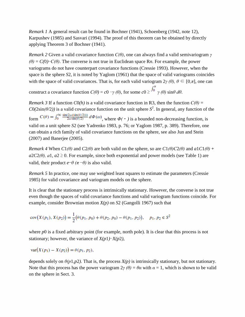
Remark 1 A general result can be found in Bochner (1941), Schoenberg (1942, note 12), Karpushev (1985) and Sasvari (1994). The proof of this theorem can be obtained by directly applying Theorem 3 of Bochner (1941).

Remark 2 Given a valid covariance function C(θ), one can always find a valid semivariogram γ (θ) = C(0)−C(θ). The converse is not true in Euclidean space Rn. For example, the power variograms do not have counterpart covariance functions (Cressie 1993). However, when the space is the sphere S2, it is noted by Yaglom (1961) that the space of valid variograms coincides with the space of valid covariances. That is, for each valid variogram 2γ (θ), θ ∈ [0,π], one can

construct a covariance function C(θ) = c0 −γ (θ), for some c0 ≥ γ (θ) sinθ dθ.

Remark 3 If a function C0(h) is a valid covariance function in R3, then the function C(θ) = C0(2sin(θ/2)) is a valid covariance function on the unit sphere S2. In general, any function of the

form , where Φ(・) is a bounded non-decreasing function, is valid on a unit sphere S2 (see Yadrenko 1983, p. 76; or Yaglom 1987, p. 389). Therefore, one can obtain a rich family of valid covariance functions on the sphere, see also Jun and Stein (2007) and Banerjee (2005).

Remark 4 When C1(θ) and C2(θ) are both valid on the sphere, so are C1(θ)C2(θ) and a1C1(θ) + a2C2(θ), a1, a2 ≥ 0. For example, since both exponential and power models (see Table 1) are valid, their product e−θ (π −θ) is also valid.

Remark 5 In practice, one may use weighted least squares to estimate the parameters (Cressie 1985) for valid covariance and variogram models on the sphere.

It is clear that the stationary process is intrinsically stationary. However, the converse is not true even though the spaces of valid covariance functions and valid variogram functions coincide. For example, consider Brownian motion X(p) on S2 (Gangolli 1967) such that

where p0 is a fixed arbitrary point (for example, north pole). It is clear that this process is not stationary; however, the variance of X(p1)−X(p2),

depends solely on θ(p1,p2). That is, the process X(p) is intrinsically stationary, but not stationary. Note that this process has the power variogram 2γ (θ) = θα with α = 1, which is shown to be valid on the sphere in Sect. 3.

In this section, we check the validity of some commonly used covariance and variogram functions. A summary of all results is presented in Table 1.

Table 1 Validity (positive definiteness) of covariance functions on the sphere, a >0, θ ∈ [0,π]

Model Covariance function Validity Spherical

Yes

Stable

Yes for α ∈ (0, 1] No for α ∈ (1, 2]

Exponential

Yes

Gaussian No Powera c0 − (θ/a)α Yes for α ∈ (0, 1] No for α ∈

(1, 2] Radon transform of order 2 e−θ/a(1+ θ/a) No Radon transform of order 4 e−θ/a(1+ θ/a +θ2/3a2) No Cauchy (1+ θ2/a2)−1 No Hole-effect sin aθ/θ No aWhen α ∈ (0, 1], power model is valid on the sphere for some (θ/a)α sinθ dθ

3.1 Spherical Model

A spherical covariance function has the form

where a > 0 is a scale parameter. This model is valid in [eqnR]1, [eqnR]2 and [eqnR]3 (Cressie 1993). To check whether it is valid on the sphere, we compute the coefficients bn in (2) through the following sine expansion of the Legendre polynomials (Hobson 1931, p. 20; also 8.826.1 in Gradshteyn and Ryzhik 1994):

More compactly, , where

Then,

Where, for integer (g(n + 2k) −g(n

+2k + 2)). Here, we define, for . To show that bn ≥ 0 for all n ≥ 0, it is sufficient to show that bnk ≥ 0. Evaluating the integral for g(x) and then taking its

first derivative leads to . This indicates that g(x), x > 0, is non-increasing, implying that .

Next we show that Σn bn <∞. We first apply the mean value theorem to obtain for k ≥ 0, where C1 > 0 is a constant independent of n and k (for notational simplicity, the same C1 will be used throughout this section, even if each instance of C1 may not be the same). In addition, observing that

and applying the Sterling’s approximation to factorials for sufficiently large n, we have

Hence, for n large, , implying Σnbn <∞. Therefore, the spherical covariance function is valid on the sphere.

3.2 Stable Model and Power Model

In this subsection, we consider the stable covariance function (Chilès and Delfiner 1999)

and the power variogram function (Cressie 1993)

Both functions are invalid when α > 2 but valid when α ∈ (0, 2] in n (Yaglom 1987). The exponential and Gaussian models are special cases of the stable model (5), corresponding to α =

1 and α = 2, respectively. Note that the function γ (・) is conditionally negative definite if and only if e−λγ (・) is positive definite for any λ > 0 (Schoenberg 1938). Therefore, it is equivalent to check the validity of the stable covariance function and the power variogram function. In addition, by Remark 2 in Sect. 2, it is also equivalent to check the power variogram function and the function

for some . We termC(θ) in (7) the power covariance function. In summary, it is equivalent to check the validity among these three covariance and variogram functions.

We focus our discussion on validity of these functions when α ∈ (0, 2]. Wood (1995) and Gneiting (1998) show that the stable covariance function is not valid on the circle when α ∈ (1, 2]. Therefore, the stable covariance function is not valid on the sphere, since a valid covariance function on the sphere will always be valid on the circle (Schoenberg 1942). When α ∈ (0, 1], in Appendix we show that the power covariance function (7) is valid on the sphere.

Our findings are summarized in Table 1. The stable covariance function and power variogram are valid when α ∈ (0, 1], but not valid when α ∈ (1, 2]. In particular, the exponential covariance function exp{−θ/a} is valid, and equivalently the power variogram 2γ (θ) = θ/a is also valid. However, the Gaussian covariance function exp{−(θ/a)2} is not valid (see also Gneiting 1999). Note that power models with α >1 are not uncommon in practice. Janis and Robeson (2004) estimated over 300 period-of-record variograms using the power model, with approximately 26% having α >1.

3.3 Other Models

In this subsection, we check the validity of the following covariance functions: Radon transforms of exponential model (orders 2 and 4), Cauchy model, and hole-effect model. The computations are carried out by directly checking some of the coefficients bn in (2).

3.3.1 Radon Transforms of Exponential Model

The following two Radon transforms of exponential model (orders 2 and 4) can be found in Chilès and Delfiner (1999, p. 85) and Gneiting (1999)

By direct computation, we found that b6 < 0 for C1(θ), and b2 < 0 for C2(θ), when a = 1. Therefore, neither is a valid covariance function on the sphere.

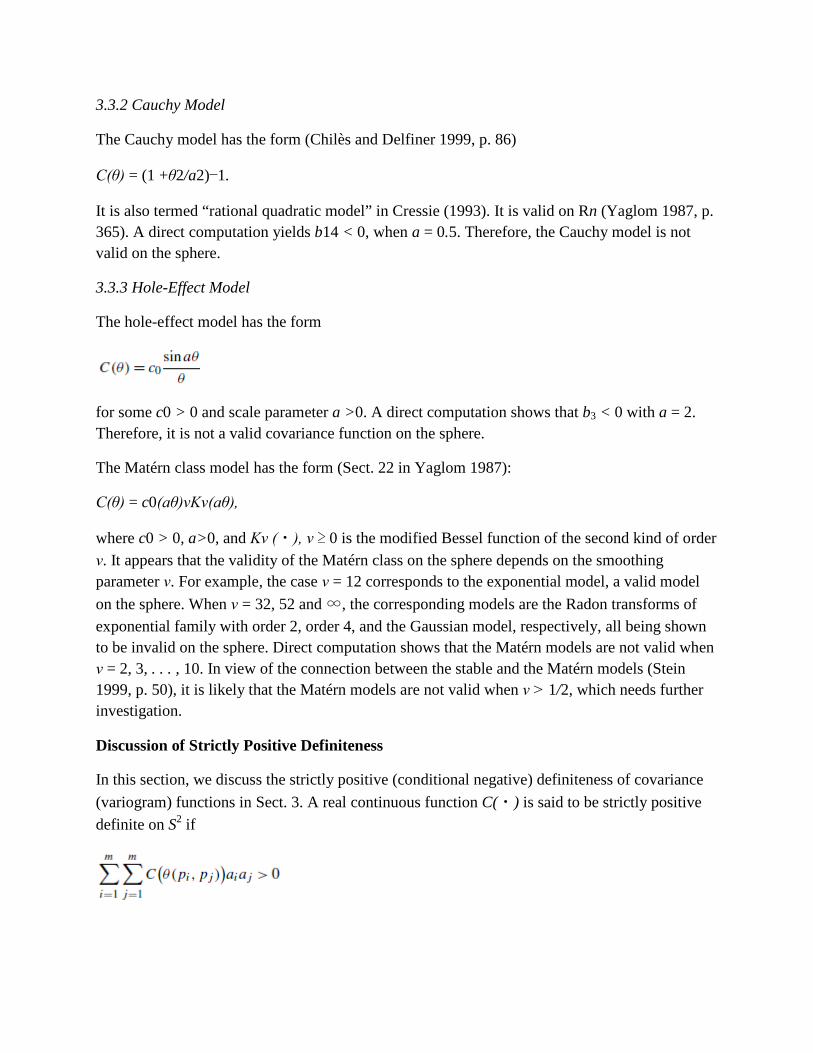
3.3.2 Cauchy Model

The Cauchy model has the form (Chilès and Delfiner 1999, p. 86)

C(θ) = (1 +θ2/a2)−1.

It is also termed “rational quadratic model” in Cressie (1993). It is valid on Rn (Yaglom 1987, p. 365). A direct computation yields b14 < 0, when a = 0.5. Therefore, the Cauchy model is not valid on the sphere.

3.3.3 Hole-Effect Model

The hole-effect model has the form

for some c0 > 0 and scale parameter a >0. A direct computation shows that b3 < 0 with a = 2. Therefore, it is not a valid covariance function on the sphere.

The Matérn class model has the form (Sect. 22 in Yaglom 1987):

C(θ) = c0(aθ)νKν(aθ),

where c0 > 0, a>0, and Kν (・), ν ≥ 0 is the modified Bessel function of the second kind of order ν. It appears that the validity of the Matérn class on the sphere depends on the smoothing parameter ν. For example, the case ν = 12 corresponds to the exponential model, a valid model on the sphere. When ν = 32, 52 and ∞, the corresponding models are the Radon transforms of exponential family with order 2, order 4, and the Gaussian model, respectively, all being shown to be invalid on the sphere. Direct computation shows that the Matérn models are not valid when ν = 2, 3, . . . , 10. In view of the connection between the stable and the Matérn models (Stein 1999, p. 50), it is likely that the Matérn models are not valid when ν > 1/2, which needs further investigation.

Discussion of Strictly Positive Definiteness

In this section, we discuss the strictly positive (conditional negative) definiteness of covariance (variogram) functions in Sect. 3. A real continuous function C(・) is said to be strictly positive definite on S2 if

for any finite number of distinct spatial locations {pi, i = 1, . . . , m} on S2 and real numbers {ai, i = 1, . . . , m}. A parallel definition for strictly conditional negative definiteness can be given as well.

There is a rich discussion in the literature about the strictly positive (conditional negative) definiteness of a continuous function on the sphere (e.g. the sufficient conditions in Xu and Cheney 1992 and Schreiner 1997, and the necessary conditions in Chen et al. 2003). Here, we summarize our findings as the following.

The sufficient condition for strictly positive definite functions on a sphere is that bn in the expansion (1) should be positive with a finite number of them being zero (e.g. Xu and Cheney 1992; Schreiner 1997). By inspecting the coefficients bn for the power model in Appendix, one can conclude that all the coefficients bn are positive when 0 < α < 1, which leads to the strictly positive definiteness. In parallel, the spherical covariance function is also strictly positive definite on the sphere.

The case of α = 1 in the power model yields the coefficients ((8) in Appendix) to be zero for all even terms and positive for all odd terms, which does not satisfy the necessary condition in Chen et al. (2003). Therefore, it is not strictly positive definite on the sphere, even though it is positive definite. Consequently, the power variogram γ (θ) = θ is not strictly conditionally negative definite. As an example, we consider such an intrinsic stationary process X(p), p ∈ S2, at four locations: north pole (pN), south pole (pS ) and two points on the equator, pE and pW, such that θ(pE,pW) = π. It is clear that var(X(pN)+ X(pS)− X(pE)− X(pW)) = 0.

The stable model exp(−(θ/a)α), 0<α <1, a>0, is strictly positive definite on the sphere. The case of α = 1, corresponding to the exponential covariance function C(θ) = exp(−θ/a), a > 0, is also strictly positive definite, since the coefficients for all n, where bnk can be shown to be

Acknowledgements We are grateful for the comments from the associate editor and anonymous reviewers, which have helped to improve this manuscript tremendously. We would also like to express special thanks to an anonymous reviewer who suggested the investigation of strictly positive (conditional negative) definiteness of covariance (variogram) functions on the sphere. Chunfeng Huang’s research is supported by the National Science Foundation DMS 0808993.

Appendix: Validity of Power Covariance Functions

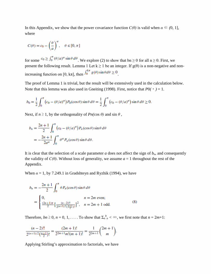
In this Appendix, we show that the power covariance function C(θ) is valid when α ∈ (0, 1], where

for some . We explore (2) to show that bn ≥ 0 for all n ≥ 0. First, we present the following result. Lemma 1 Let k ≥ 1 be an integer. If g(θ) is a non-negative and non-

increasing function on [0, kπ], then .

The proof of Lemma 1 is trivial, but the result will be extensively used in the calculation below. Note that this lemma was also used in Gneiting (1998). First, notice that P0(・) = 1.

Next, if n ≥ 1, by the orthogonality of Pn(cos θ) and sin θ ,

It is clear that the selection of a scale parameter a does not affect the sign of bn, and consequently the validity of C(θ). Without loss of generality, we assume a = 1 throughout the rest of the Appendix.

When α = 1, by 7.249.1 in Gradshteyn and Ryzhik (1994), we have

Therefore, bn ≥ 0, n = 0, 1, . . . . To show that Σnbn < ∞, we first note that n = 2m+1:

Applying Stirling’s approximation to factorials, we have

for some constant C1 > 0 independent of m (each appearance of C1 above may not be the same). Hence,Σn

bn <∞, implying that C(θ) = c0 − θ is a valid covariance function for some

=π. Consequently, the exponential covariance function exp{−θ} is valid, so is the power variogram 2γ (θ) = θ.

When 0<α <1, based on the sine expansion (3) of Pn(cos θ), we can write

where Dnk > 0 is given by (4), and

First, the proof of Σnb

n <∞can be followed along the same lines with those for the spherical

covariance function with , for large n and k. Therefore, to prove the validity of C(θ), it is sufficient to show that bn ≥ 0, or in turn, that bnk ≤ 0 for all k ≥ 0.

Now for any n ≥ 1, k ≥ 0, by the trigonometry identity and integration by parts,

From Lemma 1, the first term in (9) is non-positive for any n ≥ 1, k ≥ 0. To prove that the second term is non-positive, we explore the cases of n + 2k being odd or even.

When n + 2k is odd, by substitution u = θ − (n + 2k)π, the integral of second term in (9) becomes

implying that bnk < 0 by Lemma 1.

When n+2k = 2m is an even number for some m ≥ 1, substituting n+2k +2 = 2m+2 and n+2k = 2m into (9), we have

where

From Lemma 1, to prove bnk < 0 and hence conclude the whole proof, it is now sufficient to show that g(θ) is non-negative and non-increasing.

To show that g(θ) ≥ 0, we recall that for 0<α <1, θα−1 is a decreasing function

To show that g(θ) is non-increasing, we take the first derivative of g(θ) with respect to θ , and note that α −1 < 0

Therefore, g(θ) is non-increasing, concluding the proof.

References

Alkhaled AA, Michalak AM, Kawa SR, Olsen SC, Wang JW (2008) A global evaluation of the regional spatial variability of column integrated CO2 distributions. J Geophys Res 113:D20303. doi:10.1029/2007JD009693

Banerjee S (2005) On geodetic distance computations in spatial modeling. Biometrics 61:617–625

Bochner S (1941) Hilbert distances and positive definite functions. Ann Math 42:647–656

Carmona-Moreno C, Belward A, Malingreau JP, Hartley A, Garcia-Algere M, Antonovskiy M, Buchshtaber V, Pivovarov V (2005) Characterizing interannual variations in global fire calendar using data from Earth observing satellites. Glob Change Biol 11:1537–1555

Chen D, Menegatto V, Sun X (2003) A necessary and sufficient condition for strictly positive definite functions on spheres. Proc Am Math Soc 131:2733–2740

Chilès JP, Delfiner P (1999) Geostatistics. Wiley, New York

Cressie N (1985) Fitting variogram models by weighted least squares. Math Geol 17:563–586

Cressie N (1993) Statistics for spatial data. Wiley, New York

de BoyerMontégut C, Madec G, Fischer AS, Lazar A, Iudicone D (2004) Mixed layer depth over the global ocean: an examination of profile data and a profile-based climatology. J Geophys Res 109:C12003. doi:10.1029/2004JC002378

Gangolli R (1967) Positive definite kernels on homogeneous spaces and certain stochastic processed related to Levy’s Brownian motion of several parameters. Ann Inst Henri Poincaré, B Calc Probab Stat 3:121–226

Gneiting T (1998) Simple test for the validity of correlation function models on the circle. Stat Probab Lett 39:119–122

Gneiting T (1999) Correlation functions for atmospheric data analysis. Q J R Meteorol Soc 125:2449–2464

Gradshteyn IS, Ryzhik IM (1994) Tables of integrals, series, and products, 5th edn. Academic Press, New York

Haylock MR, Hofstra N, Klein Tank AMG, Klok EJ, Jones PD, New M (2008) A European daily high resolution gridded data set of surface temperature and precipitation for 1950–2006. J Geophys Res 113:D20119. doi:10.1029/2008JD010201

Hobson E (1931) The theory of spherical and ellipsoidal harmonics. Cambridge University Press, Cambridge

Isaaks EH, Srivastava RM (1989) Applied geostatistics. Oxford University Press, New York

Janis MJ, Robeson SM (2004) Determining the spatial representativeness of air-temperature records using variogram-nugget time series. Phys Geogr 25:513–530

Jun M, Stein ML (2007) An approach to producing space-time covariance functions on spheres. Technometrics 49:468–479

Karpushev SI (1985) Conditionally positive-definite functions on locally compact groups and the Levy–Khinchin formula. J Math Sci 28:489–498

Kitandis PK (1997) Introduction to geostatistics. University of Cambridge Press, Cambridge

Reguzzoni M, Sanso F, Venuti G (2005) The theory of general kriging, with applications to the determination of a local geoid. Geophys J Int 163:303–314

Robeson SM (1997) Spherical methods for spatial interpolation: review and evaluation. Cartogr Geogr Inf Syst 24:3–20

Sasvari Z (1994) Positive definite and definitizable functions. Akademie Verlag, Berlin

Schäfer-Neth C, Paul A, Mulitza S (2005) Perspectives on mapping the MARGO reconstructions by variogram analysis/Kriging and objective analysis. Quat Sci Rev 24:1083–1093

Schoenberg IJ (1938) Metric spaces and positive definite functions. Trans Am Math Soc 44:522–536

Schoenberg IJ (1942) Positive definite functions on spheres. Duke Math J 9:96–108

Schreiner M (1997) On a new condition for strictly positive definite functions on spheres. Proc Am Math Soc 125:531–539

Stein ML (1999) Interpolation of spatial data. Springer, New York

Webster R, Oliver M (2001) Geostatistics for environmental scientists. Wiley, Chichester

Wood ATA (1995) When is a truncated covariance function on the line a covariance function on the circle? Stat Probab Lett 24:157–164

Xu Y, Cheney EW (1992) Strictly positive definite functions on spheres. Proc Am Math Soc 116:977–981

Yadrenko MI (1983) Spectral theory of random fields. Optimization Software, Inc., Publications Division, New York

Yaglom AM (1961) Second-order homogeneous random fields. In: Proceedings of 4th Berkeley symposium on mathematical statistics and probability, vol 2, pp 593–622

Yaglom AM (1987) Correlation theory of stationary and related random functions. Springer, New York