on the use and misuse of child height-for-age z...
TRANSCRIPT

On the Use and Misuse of Child Height-for-AgeZ-score in the Demographic and Health Surveys
Joseph R. Cummins∗
Department of EconomicsUniversity of California, Davis
August 19, 2013
Abstract
This paper addresses the problem of model misspecification biaswhen estimating cohort-level determinants of child height-for-age z-score (HAZ) using data from the Demographic and Health Surveys(DHS). I show that the combination of DHS survey design and thebiological realities of child health in developing countries create an ar-tifact that can strongly bias regression estimates when identificationrelies on seasonal, annual or spatio-temporal variation associated witha subject’s birth cohort. I formalize the econometric problem and showthat flexible specifications of the HAZ-age profile can greatly mitigatethe bias. When regression models can exploit within-cohort variationin the covariate of interest, appropriate fixed-effects models can effec-tively purge the bias. I also provide Monte Carlo evidence that DHSrecommended inference strategies produce standard errors that are toosmall when estimating birth cohort determinants of HAZ.
∗I would like to thank Hilary Hoynes, Douglas Miller, and Steve Vosti for helpful com-ments on previous drafts. I would also like to thank Kathryn Dewey, Edward Miguel, Man-isha Shah, Tania Barham, Jorge Aguero, Adrian Barnett, Bruno Schoumaker and Tom Voglfor helpful conversations and encouragement, and seminar participants at UC Davis, UCBerkeley, and the Pacific Development Conference. All mistakes, conceptual shortcomings,and methodological imperfections are my own.
1

On the Use and Misuse of HAZ in the DHS 2
1 Introduction
I demonstrate how a statistical artifact in Demographic and Health Survey
(DHS) data can bias regression estimates of cohort determinants of child
height-for-age Z-score (HAZ). The short survey window of the DHS and the
relatively long periods between survey rounds induce a mechanical, cyclical
relationship in the data between birth cohort and age-at-measurement. Sep-
arately, the biological effects on children of chronic undernutrition and poor
health cause a rapid loss of HAZ over the first few years of life, generating
a strong, non-linear relationship between HAZ and age-at-measurement (the
HAZ-age profile). Together, survey design and biology conspire to induce a
spurious correlation in the data between birth cohort and HAZ that is driven
by age-at-measurement and specifically determined by the particular dates on
which the various survey rounds were conducted. The artifact is likely to bias
coefficient estimates when the HAZ-age profile is misspecified in specific but
common ways.
I refer to this relationship between birth cohort and HAZ as the timing
artifact. As a general condition, the artifact arises when data is collected in-
frequently over a short period of time on an outcome variable that is itself
a function of age. After providing the necessary background (Section 2), I
formalize the econometric problem in the context of estimating cohort deter-
minants of HAZ in the DHS, and interpret the bias in an omitted variables
framework (Section 3). I consider two means of eliminating the bias: flexible
specification of the HAZ-age profile, and identification based on within-cohort
variation. Choice of strategy by the practitioner will depend primarily on the
nature of the data the researcher is able to bring to bear on the question, but
in general within-cohort estimates are preferable.

On the Use and Misuse of HAZ in the DHS 3
I then demonstrate the artifact and bias empirically in two environments
(Section 4): estimating the effects of month of birth in Bangladesh and GDP
per capita in year of birth in Zimbabwe. In the month of birth example, a
regression with no control for age that ignores the relationship between month
of birth and age-at-measurement estimates the peak-to-trough difference in
seasonal effects at a statistically significant .245 standard deviations (p = .017
). A more flexible model that specifies a spline control across age estimates a
statistically insignificant peak-to-trough difference of .131 standard deviations
(p = .414 )1, a decrease in magnitude of about 45%. In the GDP regressions,
moving from no control for age to a spline specification reduces the implied
effect of a 10% increase in GDP from .11 standard deviations to .03.
Following the empirical examples, I present results from a placebo-type
Monte Carlo exercise simulating a “random weather shock” on data from Peru
(Section 5). I find that cohort and region fixed-effects estimators that simul-
taneously harness geographic and temporal variation can fully purge the bias,
but that estimators relying purely on temporal variation and flexible paramet-
ric specifications of the HAZ-age profile remain mildly biased.
The empirical and simulated exercises also provide evidence that DHS
recommended standard error calculations, which account only for survey sam-
pling and weighting (Madise et al., 2003), produce standard errors that tend
to over-reject a true null hypothesis when estimating cohort effects2. Sug-
gestively, between 40% and 80% of other countries’ GDP time-series appear
significantly correlated with the height of Zimbabwean children at the 95%
1P-values are for F-stats testing Feb-Dec point estimates jointly 0 using DHS recom-mended inference accounting for weighting, stratification and cluster sampling.
2The simulation design and statistical theory closely follow Bertrand et al. (2004), whichinvestigates standard error properties using the Current Population Survey in the UnitedStates.

On the Use and Misuse of HAZ in the DHS 4
level when DHS recommended standard errors are employed. These “rejection
rates” decrease to between .03 and .09 when more conservative wild cluster-
t bootstrap procedures are used to determine statistical significance. In the
Monte Carlo environment, where rejection rates of .05 can be known to be
expected, DHS standard error estimates lead to rejection rates of around .25
at 95% confidence. Alternative strategies that rely on cluster-robust analytic
methods yield more appropriate rejection rates of around .08.
2 Background
Early life and in utero exposure to environmental and economic stresses has
lasting effects on human capital development (Almond and Currie (2011),
Uauy et al. (2011)). However, the mechanisms by which these early life condi-
tions leave their mark are not well understood (Rasmussen, 2001). By tracking
persistent birth cohort effects through all stages of life, researchers hope to
flesh out the biological and socioeconomic mechanics behind the correlations
between early life environment and later life economic success (Glewwe and
Miguel, 2008). Methodologically, this literature has focused on accounting
for important behavioral considerations like endogenous fertility, unobserved
household characteristics, and/or non-random mortality (Strauss and Thomas
(1995) ; Pitt (1997)). Previous research using the DHS has also mentioned
the difficulty in effectively controlling for the HAZ-age profile (e.g. Paxson
and Schady (2005), Aguero and Valdivia (2010)), though no prior work has
provided a formal analysis of the problem.
This paper focuses on HAZ, an age- and gender-normalized measure of
child height given in units of standard deviations and relative to the median
age- and gender-conditional height distribution of a well-nourished, healthy

On the Use and Misuse of HAZ in the DHS 5
population of children. HAZ is of particular interest because it both captures
the long-term cumulative effects of health throughout childhood and is known
to be correlated with later life outcomes (Dewey and Begum (2011), Hoddinott
et al. (2008)). If in utero shocks lead to permanent health effects, they should
be measurable later in life via HAZ. In addition to the examples I investigate3,
it has been used to estimate the effects of early life exposure to crop failure
(Akresh et al., 2011), violence (Akresh et al., 2012), access to health facilities
(Valdivia (2002)), agricultural price shocks (Cogneau and Jedwab (2012), and
a number of other birth cohort HAZ determinants.
HAZ is often described as “age-adjusted height”4. However, age may
be the single best predictor of HAZ available for children in less developed
countries. Figure 1 shows the HAZ-age profile for the three countries I analyze
here - Bangladesh, Zimbabwe and Peru - with mean HAZ plotted across child
age in months. In the first two years of life children in Bangladesh lose about
1.5 standard deviations of HAZ. By way of comparison, Bangladeshi children
born to households in the highest asset index quintile are about 1 standard
deviation taller than those born to parents in the lowest quintile. Bangladeshi
children with mothers in the tallest height quintile are on average 1.1 standard
deviations taller than those with mothers in the lowest quintile. HAZ as a
measure of child health in developing countries may be “adjusted for age” in
some sense, but it is also very strongly determined by age.
The DHS are natural datasets for investigating cohort determinants of
HAZ. As of 2010, standard DHS surveys had been conducted 236 times in 84
3See Lokshin and Radyakin (2012), Aguero and Valdivia (2010) and Portner (2010) forpapers examining month of birth, GDP per capita and weather shocks respectively.
4This analysis uses the 2006 WHO standards for HAZ, computed using the Stata package“haz06” and variables for age, height, and gender. I have also run most analyses usingthe previously favored NCHS/FELS/CDC standards. Choice of standardization does notqualitatively affect results.

On the Use and Misuse of HAZ in the DHS 6
countries, with 196 of the surveys similar to those analyzed here (Fabic et al.,
2012). The costs of continual demographic surveillance are high, and so for
most of the past two decades surveys have been implemented in participating
countries only every four to five years, conducted over a period of just a few
months. Continuity in cohorts between surveys is achieved by recording data
on all children under the age of 5 found in sample households.
Use of the DHS has increased steadily. Fabic et al. (2012) finds 1177
journal articles published using DHS data between 1985 and 2010, and this
count relies only on articles found on the measureDHS website and on PubMed.
The rate at which articles using DHS data are published is also increasing,
from less than 50 per year in 2000 to almost 150 per year in 2010. A little over
half of these publications dealt with maternal and child health in general, and
by 2010 there were around 25 papers per year being published on nutritional
deficiencies, where the primary outcome is likely to be HAZ or some other
anthropometric outcome.
3 Econometric Demonstration
This paper is focused on estimating the effects of birth cohort regressors on
HAZ, but the econometric problem is not restricted to the particular outcome
or dataset. Three ingredients are required for the timing artifact to bias re-
gression estimates: 1) the data being analyzed comes from measurements of
subjects taken over a short period of time at infrequent intervals; 2) the out-
come variable of interest must be in part determined by the subjects’ ages;
and 3) the covariate of interest must be measured in relation to the subjects’
birth cohorts, for example a birth year or birth quarter aggregate variable.
The data collection method (1) ensures that cohort and age-at-measurement

On the Use and Misuse of HAZ in the DHS 7
are mechanically related in a manner determined by the dates on which the
measurements were taken and the ages of the population of interest. The
outcome-age profile (2) translates this age-cohort relationship into a spurious
outcome-cohort relationship - the timing artifact. When estimating the effects
of some cohort level variable (3), failure to adequately control for the outcome-
age profile can allow residual, spurious variation in cohort HAZ (induced by
the timing artifact) to induce an omitted variables bias on regression estimates.
Intuitively, the least squares machinery associates the spurious timing artifact
variation in HAZ with the time series variation in the birth cohort variable of
interest. This problem is particularly worrisome when there are only a small
number of cohorts (and thus no law of large numbers for “randomization”
across cohorts) and/or there is temporal serial-correlation in the time series of
the covariate of interest (since the spurious time series component of cohort
HAZ induced by the timing artifact is also serially-correlated across time).
3.1 Intuition Using Month of Birth
The most basic form of the econometric problem is to estimate the effect of
a birth cohort variable of interest βT on some partially age-determined out-
come Y, when data for estimating βT comes from a random cross-section of
the population of interest, and measurements are taken simultaneously and in-
stantaneously on all sample subjects. Suppose real world data were generated
in the following manner:
Yia = X ′iaβx + βT ∗ Ta + f(age) + εia (1)
Y, for individual i of age a, is determined by some set of covariates X, a
covariate of interest (or treatment) T, the subject’s age at measurement, and

On the Use and Misuse of HAZ in the DHS 8
an iid error term ε. T is subscripted by ‘a’ because it is an aggregate measure
common to some aspect of birth cohort, and in this framework cohort and age
are perfectly collinear. I choose to subscript using a instead of c to emphasize
that Y is partially a function of age, via f(), which is not restricted to be
well behaved in any way. This stylized model is analogous to an empirical
environment where one round of the DHS is employed, and the fact that the
survey is conducted over several months is abstracted away.
3.1.1 Timing Artifact and Month of Birth
The first task in linking the timing artifact to estimates of βT is to understand
the relationship between T and age-at-measurement in the data. To make this
relationship clear with an example, suppose T is a vector of dummy variables
for month of birth. The mechanical relationship between age-at-measurement
and month of birth makes the problem somewhat unique, but it also makes
the timing artifact visible in a way that can be obscured once an additional
layer of variation is introduced.
Assume for the moment that the survey in question was taken on January
1, 2000, at 12:01am, and that, like the DHS, it takes as a population of interest
children under the age of 5 (all children born on or after January 1, 1995). In
this case, all sample children who were born in December were measured at
ages 1 month (born December 1999), 1 year 1 month (born December 1998),
2 years 1 month (born December 1997), etc. Similarly, all children born in
June were measured at the ages of 6 months (born June 1999), 1 year and
6 months (born June 1998), etc. Because younger children have higher HAZ
than older children (due to the HAZ-age profile), December-born children are
not just younger, but also have higher HAZ than June-born children. To see

On the Use and Misuse of HAZ in the DHS 9
this graphically, consider Figure 1. In this setting, all children at the furthest
left end of the graph would be December-born children. Six months to the
right would be June-born children, who were measured at 6 months old and
thus have lower mean HAZ than the December children who were measured at
1 month old. The same pattern repeats for children aged 1 year and 1 month
(December-born) compared to children aged 1 year and 6 months (June-born),
and again for ages of 2, 3 and 4 years, though for the older ages the exact trend
is less visually apparent as the HAZ-age profile flattens5. Had the survey been
conducted in summer, the reverse would be true.
Although this stylized environment represents only a single survey taken
at a single point in time, the problem is easily generalized to include multiple
survey rounds taken over several months each and several years apart. The
left panel of Figure 2 shows survey timing in Bangladesh for four contiguous
survey rounds, with the the year of the survey on the Y-axis and the months
of the survey window (the months in which measurements were taken) plotted
on the X-axis. Early rounds (1996 & 2000) were conducted mostly in winter,
while the later rounds (2004 & 2007) were conducted in spring and summer.
On aggregate, then, children born in late fall and winter were measured at
younger ages than children born in spring. This is shown in the right panel of
the figure, which is a bar graph depicting mean age-at-measurement by month
of birth.
The effect of this imbalance of age across birth months on HAZ is repre-
sented in the top panel of Figure 3. This figure overlays a line graph of mean
HAZ by birth month on the age-at-measurement bar graph shown in Figure 2.
5Even for 3 and 4 year olds, children are losing HAZ within any age-in-years bin. This islikely a result of both the standardizing process (de Onis et al., 2004) and age misreporting(Schoumaker, 2009), and it can be seen in Figure 6 which plots the estimated HAZ-ageprofile from a spline function with separate intercepts at round age in years.

On the Use and Misuse of HAZ in the DHS 10
The sinusoidal shape of the line graph strongly resembles the canonical season
of birth graph. But the true relationship is clear from the bar graph: higher
HAZ is apparent in months where children born in that month were measured
at younger ages, and these months are the months immediately preceding the
survey timing. An even more compelling example is shown in the bottom two
panels. They show the same graph but with the sample restricted to children
measured in either February (left panel) or November (right panel), and lim-
ited to the 1996 and 2000 survey rounds which both ran roughly November
(’94/’99) to February (’96/’00). The February graph looks the same as the
November graph shifted four months forward. The entire magnitude of the
apparent birth month seasonality in child HAZ outcomes can be explained
by the survey timing induced differential in age-at-measurement across birth
months.
3.1.2 Bias
The correlation between HAZ and month of birth described above is an uncon-
ditional correlation. If we can fully control for the “natural” loss of HAZ over
age, estimates of βT should be unbiased. Common strategies to account for the
HAZ-age profile include linear or polynomial specifications in age or dummy
variables for age in months. However, misspecification of the HAZ-age profile
can induce bias in the same manner as non-specification can. To formalize the
problem econometrically, suppose that the researcher specifies a model of the
following form using data generated by Equation 1, where g(agea; γ) is some
parametric specification of f(age):
Yia = X ′iaβx + βT ∗ Ta + g(agea; γ) + ηia (2)

On the Use and Misuse of HAZ in the DHS 11
Unbiased estimation of Equation 2 requires that the error term η is un-
correlated with T. However, in the presence of misspecification of g() such
that g() does not fully control for f(), analysis of the underlying data gen-
erating process shows this to be an unreasonable assumption. Returning to
Equation 1, I add and subtract g(), producing:
Yia = X ′iaβx + βT ∗ Ta + g(agea; γ) + [f(age) − g(agea; γ)] + εia (3)
Define µa = f(age)−g(agea; γ), the age-invariant systematic error in the
estimate of f() across age. Since both f() and g() are functions only of age, µa
is then also solely a function of age and all subjects with the same age have the
same value of µ. While η in the estimating equation was posited as being iid
(as being ε), this exercise allows us to decompose η into two components: ε, the
real-world iid error, and µ, the model misspecification error component that
is the age-conditional difference between f() and g(). Plugging this definition
of η back into Equation 2, we see that the equation the researcher ought to be
estimating is:
Yia = X ′iaβx + βT ∗ Ta + g(agea; γ) + µa + εia (4)
To simplify the analysis, assume that f() is a linear combination of some
set of age-transformations (age, its square, discontinuities, etc.), and that g()
does not contain one or more of these transformations. µ can now be under-
stood as an omitted variable in the original specification of Equation 2. As
the classical demonstration of omitted variables bias shows6, coefficient esti-
6see Angrist and Pischke (2008) pages 59-61 for proof and discussion.
On the Use and Misuse of HAZ in the DHS 12
mates on any variables included in the regression that are correlated with µ
will be biased. Such a correlation does not require a particularly anomalous
situation. In cases where f() is smooth and g() is specified to be smooth, µ
will be smooth, and thus serially-correlated across age, and thus T and µ will
likely move together (or against each other) in one fashion or another over at
least some periods of time.
3.2 Two Strategies for Unbiased Estimation
In this subsection I discuss two approaches to purging regression estimates of
timing artifact-induced bias. The choice of strategy by the researcher will de-
pend largely on the types of identifying variation in the birth cohort variable
the researcher can bring to bear on the problem. The first strategy is directly
implied by the discussion above and the framing of the omitted variables bias
interpretation: minimize the potential impact of µ through flexible specifica-
tion of g(). This turns out, for reasons discussed in the following section, to
be a more problematic approach than it first appears.
The second strategy hinges on the realization that model misspecification
itself is not always problematic, even model misspecification that is invariant
across age. The problem arises not only because µ is age-invariant, but also
because age is correlated with T. In the presence of within-cohort variation
in T, such as regional or subject-level quasi-experimental variation, it may
be possible to separate out the cohort/age effect from the effect of T within
each cohort, and thus achieve identification based on assumptions about the
distribution of age (and hence the distribution of µ), within cohort, across T.

On the Use and Misuse of HAZ in the DHS 13
3.2.1 Flexible Specification of g()
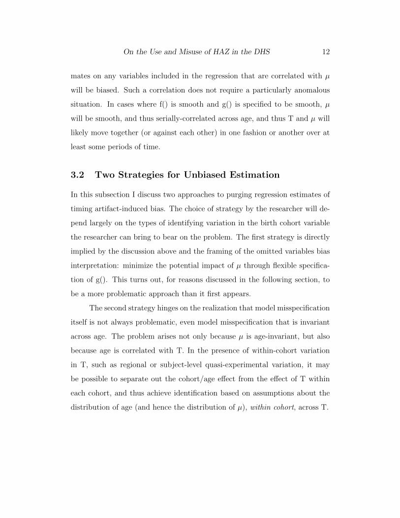
One way to visualize the timing artifact is to plot out the HAZ “time-series”
produced using DHS data by collapsing mean HAZ by date of birth. I show this
in Figure 4. In the left panel I graph mean HAZ by birth date (aggregated
to birth month), and in the right panel I provide the same graph disaggre-
gated by survey round. While the left panel produces a graph that looks like
a plausible, even if oddly sinusoidal, time-series, the right panel reveals the
true dynamic. Most of the large variation seen in the aggregate time series is
actually caused by overlapping survey windows. When the data is disaggre-
gated, the graph appears in a more interpretable form - as the HAZ-age profile
repeating (backwards) over time.
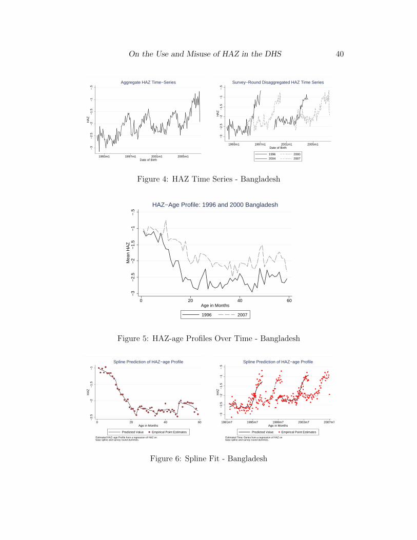
Figure 4 also raises a new modeling concern, the changing shape of this
profile over time. To show this more clearly, Figure 5 overlays the sample
mean HAZ-age profile from the first (1996) and last (2007) Bangladesh survey
rounds. Over time, children are losing HAZ less rapidly during the first few
years of life. This secular improvement in child-health affects both the shape
and the level of the HAZ-age profile across survey rounds. Any attempt to
absorb f() via g() must contend not only with the shape of the HAZ-age profile
over age, but with the secular shifting of the HAZ-age profile over time.
To formalize these considerations, suppose data in the real world were
generated in the following form, and gathered from a repeated cross section
of S survey rounds, which are now each taken over several months, but taken
several years apart:
Yiacs = X ′iacsβx + βT ∗ Tc + f(agea, birthdatec) + εiacs (5)
Y is determined for individual i of age a born into cohort c and surveyed

On the Use and Misuse of HAZ in the DHS 14
(measured) in round s. The incorporation of multiple survey rounds through
the inclusion of a more refined timing-index is the first important difference
between this model and the stylized model discussed above. The second dif-
ference is that f() is no longer conceived as simply a function of age but also
as a function of birthdate, to capture the changes in the HAZ-age profile over
time.
Ignoring the shifts in the HAZ-age profile over time will generate a second
type of model misspecification that may also induce a correlation between T
and µ. Suppose that secular improvements in child health are raising the
HAZ-age profile over time and that g() is specified as static. µ now becomes a
function of both age and time, the model misspecification associated with g()
improperly fitting the shape of the HAZ-age profile (µ in the stylized model),
as well as the systematic error that is generated across survey rounds caused
by the failure to account for the level changes over time. If not just the level
but the shape of the profile is changing over time proper specification of g()
becomes even more difficult.
An obvious assumption that would allow the researcher to identify βT is
that f() is separable into f1(age) and f2(birthdate), the assumption underlying
the inclusion of both flexible controls for age and a set of secular calendar-time
controls. These two options underlie the bulk of the previous empirical work
referenced in this paper.
A second option is to assume that one can directly model the changes
in f() over time. For example, one could specify a spline function that shifts
parametrically over time with different changes in the slopes of the spline
segments for different age groups. Since very young children have HAZ much
closer to the reference population median, there is little reason to believe that
the mean HAZ of 1 month olds is likely to increase rapidly due to some secular

On the Use and Misuse of HAZ in the DHS 15
force. However, secular health improvements are quite likely to slow the loss
of HAZ over the first few years of life.
3.2.2 Within-Cohort Variation in T
The second strategy for purging estimates of timing-artifact induced bias is
to accept the problem of model misspecification but to specify the model in
such a way that µ becomes orthogonal to T. In the environments described
above, all children born at the same time had the same value of T. This forced
identification of βT to rely on assumptions about the shape of f() and/or its
movement over time. However, it is often the case that the researcher faces a
problem where within-cohort variation in T is available or such variation can
be constructed in some manner by bringing more refined data to the problem.
Suppose data were generated in the following form:
Yiacrs = X ′iacrsβx + βT ∗ Tcr + f(agea, birthdatec) + εiacrs (6)
This process is exactly the same as that described by Equation 5 except
for the inclusion of subscript r denoting region of birth, and the fact that T
now varies within birth cohort (across regions). In this situation a cohort and
region fixed effects model can be specified. The cohort fixed effects are used to
assure the similarity of the distribution of child ages between treatment and
control. They are not functioning as a specification of g(), since the magnitude
of µ is not a concern and the fit of the model to any individual child is not
important. They are functioning instead of a specification of g(), rendering it
unnecessary by exploiting variation such that µ becomes uncorrelated with T.

On the Use and Misuse of HAZ in the DHS 16
3.3 Inference
The bulk of this paper is concerned with the question of model-misspecification
bias in estimates of βT , but the question of statistical inference is also im-
portant. Most work on standard error calculations and inference properties
using the DHS has focused on accounting for survey design: sample selection
(stratification and clustering) and population-probability weighting. Madise
et al. (2003) demonstrates that failure to account for survey design can lead
to greatly underestimated standard error estimates, giving researchers false
confidence in the statistical significance of their results.
Madise et al. (2003) focuses on estimating standard errors for the effects
of child, maternal and socioeconomic variables on child nutritional status.
That context is different in theoretically important ways from the context of
estimating standard errors for the effects of birth cohort aggregate variables.
In this environment there is likely to be strong serial correlation in the regressor
of interest within birth cohort or region. Bertrand et al. (2004) demonstrates
that ignoring such serial correlation can lead to standard error estimates that
are much too small.
Serial correlation is usually addressed spatially by clustering on the
“cross-sectional” variable, in this case region. This is the environment in
which Bertrand et al. (2004) and Cameron et al. (2008) operate. But in the
context of birth cohort aggregate variables, the obvious serial correlation in
the regressor of interest is temporal. I thus investigate both temporal and spa-
tial correlation, “clustering” on either cohort or region groupings. Since the
number of cohorts is generally small (less than 40), and since cluster-robust
analytic estimators only converge in probability to the true standard error
as the number of clusters goes to infinity, I follow Cameron et al. (2008) in

On the Use and Misuse of HAZ in the DHS 17
conducting a wild cluster-t bootstrap procedure to compute p-values when
clustering on cohort or region is proper.
4 Empirical Examples
In this section I discuss two empirical contexts in which the timing artifact
can induce bias on regression estimates of cohort variables. The first example,
partially discussed in Section 3, is the effect of month of birth on HAZ. The
second is the effect of GDP per capita in year of birth. Both examples demon-
strate the fragility of point estimates to specification of g(age, birthdate), and
in both cases the point estimates attenuate towards zero as the specification
of g() becomes more flexible. The GDP example also lends itself nicely to
investigation of the inference properties of various statistical significance esti-
mators.
4.1 Data
In each empirical exercise, and for the data on which the placebo-test Monte
Carlo simulations are run, I use four waves of DHS data from three countries,
one country for each exercise - Bangladesh (month of birth) and Zimbabwe
(GDP per capita in birth year) for the empirical examples, and Peru for the
simulation exercise (weather shocks). All surveys were conducted between
1992 and 2011 (International, 2011). I aggregate all birthdates to month and
year. Sample weights are re-normalized so that each survey is weighted equally,
with relative sampling probability preserved within survey round. Results are
robust to use of original DHS weights or no weights at all. Specifics of the
sample selection and survey design are provided in Appendix A.

On the Use and Misuse of HAZ in the DHS 18
Table 1 displays unweighted summary statistics for the three example
countries. Child HAZ is lowest in Bangladesh, where the mean HAZ hovers
around the -2 standard deviations “stunting” level used internationally as a
mark of moderate, chronic malnutrition. Children in Peru and Zimbabwe have
slightly better HAZ measures, but remain more than a full standard deviation
below the reference population of well nourished children. These numbers are
consistent with many countries that face endemic disease and chronic nutri-
tional shortfalls. Maternal age, education and height, and urban/rural com-
position are also consistent with much of the developing world (Ayad et al.,
1997).
The covariates shown here, along with region dummies, constitute the
set of X covariates used in the regressions that follow. Maternal education is
entered in regressions as a set of five dummy variables7. Continuous variables
other than child age and date of birth are entered into regressions linearly.
Many papers that analyze child HAZ outcomes employ a much larger vector
of covariates. I employ a sparse set to maintain sample size and increase
transparency. Inclusion of larger covariate sets makes no qualitative difference
to the results presented.
4.2 Month of Birth in Bangladesh
The first empirical question is whether or not the theoretical bias discussed in
Section 3 actually affects point estimates to a meaningful degree after control-
ling for age. To determine the potential magnitude of the bias in an empirical
setting, and to test the ability of increasingly flexible specifications of g() to
7These are no education, primary school, secondary school, higher education, and adummy for unknown educational status. Data definitions are provided by International(2012)

On the Use and Misuse of HAZ in the DHS 19
purge the bias, I estimate month of birth effects using data from Bangladesh.
In this environment the timing artifact is likely to be quite strong since there
is no mitigating factor between cohort and the regressor of interest, in the
sense that we are not estimating something that varies by month of birth, but
the actual effect of the month of birth itself. Beyond providing an intuitive
environment for examining timing artifact-induced bias, month of birth has
been shown to be a contributing determinant to all sorts of later-life outcomes,
and various socio-biological mechanisms have been invoked to explain the cor-
relation8. Other data artifacts can also induce the appearance of some month
of birth effects9.
4.2.1 Month of Birth: Estimation
The estimating equation for month of birth, adapted from Equation 5 with
month of birth replacing T and cohort (the interaction of month and year of
birth) now omitted and subsumed by the birth month dummies, survey round
dummies and age at measurement controls, is of the form:
HAZiams = Xiamsβx +MOBm + g(agea; γ) + λs + ηiams (7)
The model conceives f(age, birthdate) as separable: the shape of f1(age)
is assumed to be constant across time, varying only in level shifts from survey
to survey as captured by λ (the specification of f2(birthdate)). I specify several
8Angrist and Krueger (1991) and Musch and Grondin (2001) use institutional explana-tions involving age-at-entry, while Buckles and Hungerman (2008) emphasize a behavioralmechanism of selection into birth timing. The development economics literature tends tofocus on biological explanations, e.g. Lokshin and Radyakin (2012), which explains seasonalbirth effects in India by in utero exposure to the monsoon rains
9Linn et al. (2011) show that estimating seasonal effects from data collected on birthsoccurring over a fixed period of time can induce the appearance of seasonal differencesin birthweight. Lewis (1989) shows that age-at-diagnosis can explain some seasonal birthpatterns in schizophrenia.

On the Use and Misuse of HAZ in the DHS 20
forms of g1(age; γ): linear, quadratic, cubic and spline.
My base spline in this context is linear between knots, with the knots
placed at round age-in-years (12 months, 24 months, 36 months and 48 months
of age). Each knot is also allowed its own intercept, which is common across
survey rounds, to account for standardization and age-reporting issues at
round ages in years10. The fit of the spline is shown in Figure 6, which graphs
out the estimated mean HAZ-age profile for Bangladesh from a regression of
HAZ on the spline described with only the survey dummies also included in
the regression. The left panel shows the fit of the spline (the line graph) on a
scatter plot of mean HAZ across age, and the right panel shows the fit across
birthdate. It is also possible to specify more flexible spline functions that di-
rectly estimate f(age, birthdate). The approach I take is to allow the slopes of
the spline to shift parametrically or non-parametrically over time.
4.2.2 Month of Birth: Results
Figure 7 plots out the point estimates from four base specifications of g(age; γ)
- no age control, linear, quadratic, and the base spline. As the flexibility
of the specification increases, the point estimates tilt towards 0 from both
directions. The peak-to-trough difference within specification reduces from
.245 without age controls, to .188 and .163 for the linear and quadratic
specifications, to .131 with the base spline controls. F-stats and P-values for
Feb-Dec jointly 0 and accounting for survey design are reported in the legend.
All continuous specifications return statistically significant results (p < .1).
The spline specification, however, returns statistically insignificant results (p =
10Since this specification is not continuous across age (due to the separate intercepts foreach age-in-years), it may be more appropriately called a “piecewise linear” specification,with cubic splines called “piecewise polynomial”. I use the term “spline” for brevity.

On the Use and Misuse of HAZ in the DHS 21
.414).
Figure 7 shows that flexible specification of g(age; γ) can mitigate timing
artifact induced bias. Whether it eliminates the bias cannot be determined
from this exercise. The separable model may be incapable of fully absorb-
ing f(), or it may be that the secular trend is improperly modeled as survey
round dummies, or it may be that the remaining seasonal pattern is real.
A priori it is difficult to argue for one particular specification of the secular
time trend or movement of the spline over another. It is possible, though, to
test whether or not in this particular case some non-separable specification of
g(age, birthdate; γ) can make the effect disappear completely.
To test models that directly specify g(age, birthdate; γ) I run a further
series of regressions, collapsing month of birth into quarter of birth. The
coarser definition of seasonality allows me to worry less about model flexibility
compromising identification, and it simultaneously smooths out the timing
artifact effect, giving the model the best chance of finding no effect. In Table 2,
I show the results of regressions of HAZ on quarter of birth, the vector X
of covariates, and several specifications of g() that more explicitly model its
movement over time.
Column 1 shows results using a simple linear in age specification includ-
ing survey round fixed effects, while Column 2 adds in quadratic and cubic
age adjustments. Column 3 shows the cubic spline results with a linear trend
in birthdate, and Column 4 uses the same spline but adds a quadratic time
trend in birthdate. Column 5 explicitly models g(age, birthdate; γ), allowing
each spline segment slope to follow a linear trend over time, while using survey
round dummies to adjust for level changes in the HAZ-age profile. Column 6
allows the spline to have independently estimated slopes for each survey round
and includes survey dummies. The bottom row of the table displays F-stats

On the Use and Misuse of HAZ in the DHS 22
and p-values testing the null hypothesis that quarters 2-4 are jointly 0 (with
quarter 1 being omitted and set to 0), using standard errors accounting for
survey design.
The primary row of interest is the row for the effect of Quarter 4 birth, as
the point estimates increase in each quarter of birth and the highest quarter
shows the effect of specification most clearly. Moving across Table 2 from
left to right, and thus increasing the flexibility of the specification of g(), the
coefficient on the Quarter 4 dummy drops by about 40%, from .1 standard
deviations to .06. The point estimate on Quarter 4 is statistically significant
across all specifications, but the F-stat testing Quarters 2-4 jointly 0 is only
rejected at the 10% level for the first four columns. When the secular trend is
allowed to be quadratic, or when the spline is allowed to parametrically bend
over time, the F-stat indicates a failure to reject the null hypothesis of no
effect. No specification makes the effect completely disappear, but increasing
the flexibility of g() consistently dampens the magnitude.
The relationship between month of birth and age creates a relationship
between the covariate of interest and HAZ that is mechanically guaranteed.
In the next section I present an example that investigates a more conventional
time-series/cohort model.
4.3 GDP per Capita in Birth Year in Zimbabwe
The DHS is also a natural dataset to investigate the in utero and very early
life effects of the business cycle on child health, e.g. Paxson and Schady
(2005) and Aguero and Valdivia (2010) on Peru, Subramanyam et al. (2011)
on India and Pongou et al. (2006) on Cameroon. The economic growth and
HAZ literature is also the first that this author knows of to wrestle with the

On the Use and Misuse of HAZ in the DHS 23
econometric problem of separating out the effects of the HAZ-age profile from
the time-series trends in the covariate of interest.11.
Figure 8 demonstrates the timing artifact graphically in the context of
a GDP/HAZ time-series analysis. Using data from Zimbabwe, I overlay the
GDP per capita time series on a disaggregated HAZ time-series similar to
Figure 4 (which uses Bangladeshi data). The obvious problem is that any
spurious correlation between the changes in GDP per capita and where the
peaks/troughs of the HAZ-age profile hit in calendar time will cause bias in
regression estimates when g() is not properly specified.
4.3.1 GDP: Estimation
The model I specify to estimate the effects of (log) GDP per capita in year of
birth, again derived from Equation 5, is:
HAZiac = Xiacβx+βgdp∗LogGDPc+g1(agea; γa)+g2(birthdatec; γc)+ηiac (8)
This specification excludes survey-round effects, instead parametrically
modeling movements in the HAZ-age profile over time. Since identifying vari-
ation necessarily comes from temporal changes in GDP, the specification of
both g1(age; γa) and g2(birthdate; γc) are important.
To test the sensitivity of this model to specification of g1(age; γa) I test
five specifications: unconditional on age, linear, quadratic, spline, and dummy
variables for age-in-months. g2() is specified as linear or quadratic. Identifying
11Paxson and Schady (2005) is the first to discuss the problem as one in which the objectof interest is the entire HAZ-age profile. It is informative that, instead of regressing HAZon GDP and estimating an elasticity, it simply compares HAZ-age profiles across surveyrounds, and conceives of the problem as identifying changes in the shape of the HAZ-ageprofile over time

On the Use and Misuse of HAZ in the DHS 24
variation comes across time, and in the continuous specifications of g() that
includes both within-survey time variation (e.g. comparing children surveyed
in 1996 and born in 1993 and 1994) along with variation in time across surveys
(e.g. comparing the 1993 cohort with the 2005 cohort surveyed later). As the
specification of g1() becomes more flexible, though, the models rely increasingly
on between-survey variation, up to the point of the dummy variables for age in
months which identify almost exclusively off between-survey variation. There
are two concerns, though, with the dummy variable specification: first, the
problem of implicitly comparing December-born and January-born children of
the same age from the same survey who faced essentially the same economic
conditions in utero but would have different values of GDP per capita in their
birth year; and second the fact that, for any given age, there are only (S =)
4 values of GDP per capita identifying the effect. The increasingly flexible
estimates utilize less and less of the available variation in GDP per capita.
An obvious compromise between a polynomial specification and the non-
parametric specification is again a spline in age. Similar to the previous section,
I set the spline to have internal knots at round ages in years with separate
intercepts at each knot. Unlike in the month of birth example, here I can
safely specify a cubic spline to allow the model to fit the non-linearity of the
HAZ-age profile as well as possible.
4.3.2 GDP: Results
In Table 3 I present the results from a regression of HAZ on the same covariates
used previously, a linear or quadratic trend in birthdate, and the specifications
of g1(age; γ) discussed above. The effect of the age controls is clear, the point
estimates dropping towards 0 with each increasingly flexible specification. The

On the Use and Misuse of HAZ in the DHS 25
unconditional regression estimates that a 10% increase in GDP per capita in
birth year is associated with a .1 standard deviation increase in child height.
Linear specifications only reduce the implied effect to about .085 standard
deviations. The addition of age squared reduces the point estimate by almost
another half, to .048 standard deviations. The spline and non-parametric
specifications, my most flexible models, return estimated effects of around .03
standard deviations, 70% smaller than the estimate from the unconditional
specification, and just over 35% less than the estimate from the quadratic
specification.
The inclusion of quadratic controls for the secular trend leads to larger
point estimates under the spline and non-parametric specifications. Point
estimates in columns 6 and 7 are about 35% larger than the point estimates
for the same specifications of g1() with linearly specified trends. One concern
with the validity of these estimates is that, given the underlying data, there will
always be a large increase in HAZ toward the very end of the time-series, since
these cohorts are always composed of very young children. Thus, it may be
that using a quadratic specification is unwise as it will become to some degree
collinear with the HAZ-age profile at the far right end of the graph. This
concern may or may not explain the increase in point estimates, and I cannot
rule out the hypothesis that the quadratic specifications are improvements
over the linear specifications.
All estimates of the effects of GDP in birth year on HAZ are statistically
significant at the 95% level or lower when standard errors only accounting
for survey design are computed. As discussed in Section 3.3, these standard
errors do not account for serial-correlation in errors within cohort or region
but outside of sampling cluster.
To provide initial evidence as to whether or not choice of inference strat-

On the Use and Misuse of HAZ in the DHS 26
egy can greatly affect our confidence level, I compute several alternative p-
values and display them in the bottom rows of Table 3. The first row, labeled
“DHS”, shows the p-value associated with the standard error estimates shown
beneath the point estimates. This can be considered a baseline p-value against
which to judge the alternatives. The second and third rows show p-values from
standard errors that employ cluster-robust analytic specifications that cluster
the data at the birth year-by-region level (210 clusters) and the survey-by-
region level (40 clusters) respectively. P-values are based on t-distributions
with degrees of freedom equal to the number of clusters minus 2. The bottom
two rows provide p-values from the wild cluster-t bootstraps that are clustered
on region and cohort separately12.
There is a great deal of dissonance between the estimated confidence
levels across inference strategies, particularly between the analytic and boot-
strap estimators. All analytic clustering strategies, save for the region-by-
survey clustering on the first dummy variable specification, return results that
are statistically significant at the 10% level. However, both bootstraps fail
to reject the null hypothesis at any standard confidence level for any of the
specifications save the non-parametric specification with a quadratic trend in
birthdate.
4.3.3 GDP: Informal Inference Test
The massive increase in the confidence interval (or, for the bootstraps, implied
confidence interval) as clusters are defined at higher levels raises the possibility
that the DHS recommended standard errors are inappropriately small. While
I more formally test these inference strategies in the next section, I first pose
12For these bootstraps I use 500 repetitions, but in the alternate-country GDP regressionsbelow I use only 300 bootstrap repetitions to save computational requirements.

On the Use and Misuse of HAZ in the DHS 27
two questions to the data. First, how often would a random GDP per capita
time-series overlaid on the Zimbabwe DHS data generate results as extreme as
those found in the real regression? Second, how often would we reject the null
hypothesis of no effect when these placebo-GDPs are used? Neither of these
can be answered perfectly, but I can provide some evidence in the empirical
context.
Determining what, exactly, constitutes a placebo GDP time-series is dif-
ficult. As opposed to generating random GDP time-series, I take a less precise
but more intuitive approach. I address both questions by estimating the im-
plied effects of other country’s GDP per capita time series on the Zimbabwean
HAZ data. First, I take GDP per capita time-series data from the World
Bank online reference for 183 countries with data on GDP from 1990 through
201113. I then regress the Zimbabwe child height data on the GDPs of these
other countries, using the base spline specification with a linear time trend
and recording the point estimates and p-values.
Figure 9 graphs a kernel density plot of the GDP point estimates from
other country’s GDPs, and a dot for the estimated effect of Zimbabwe’s own
GDP. The vertical line shows the 95-th percentile of the distribution, and the
Zimbabwe point estimate is smaller than this level. Overall, the “real” point
estimate is less extreme (in terms of absolute value) than the point estimates
obtained using 42 of 183 alternate GDPs (about 23%). This number is similar
to the p-value obtained from the preferred birth year clustered boostrap p-
value (.188).
I then tabulate the rejection rates (5% level) and present them in Ta-
ble 4. Using DHS inference methods, I find rejection rates between .39 and .84
depending on specification, with the more flexible specifications producing the
13Data was collected from data.worldbank.org

On the Use and Misuse of HAZ in the DHS 28
lower, but still too large, rejection rates. The cluster analytic standard errors
reject the null at rates between .2 and .6, again with the more flexible specifi-
cations of g() leading to lower rejection rates through the reduction of bias on
the coefficient estimate. Of particular interest, though, are the rejection rates
given by the wild cluster-t bootstraps that cluster on birth year, which reject
the null hypothesis at a rate of around .03 to .09.
The GDP per capita exercise demonstrates two things. First, the timing
artifact can bias results even when the right hand side variable of interest is
not mechanically related to age, only measured in relation to it - the value of
GDP per capita in birth year is associated with age-at-measurement, but it
need not be. Second, standard errors calculated only to account for survey
design may be too small. What is not clear from this exercise, or from the
preceding exercise using month of birth, is whether the flexible specification
of g() is fully purging the bias and whether or not any of the strategies for
estimating statistical precision produce reliable p-values.
5 Monte Carlo: “Weather Shocks” in Peru
This section presents a formal test of both proposed strategies for eliminating
timing artifact-induced bias, as well a test of the quality of various precision
estimators. To do this, I perform two Monte Carlo exercises based on data from
the Peruvian DHS, where a placebo shock with known effect of 0 is randomly
applied to children in some regions in each cohort but not to others. The use of
a “shock” indicator for a particularly severe exposure of some type or another is
common, and weather shocks exemplify the strand of the literature (del Ninno
and Lundberg (2005)). The Peruvian data is used because of the relatively

On the Use and Misuse of HAZ in the DHS 29
large number of geographic regions provided in the data (25)14, sparing the
need to define my own geographic regions and allowing for easier replication.
5.1 Simulation Design and Estimation
The spatio-temporal fixed-effects model I consider in this context is derived
from Equation 6 but drops the age subscript since the model does not directly
specify g(). It takes the following form:
HAZircs = Xircsβx + βshock ∗ Shockrc + λc + γr + ηircs (9)
If regional differences in child HAZ are essentially level differences in the
HAZ-age profile, then, conditional on a dummy for region of birth, “control”
(shock = 0) children should generate a reasonable counterfactual mean HAZ
for children in their cohort in the “treated” (shock = 1) group. The additional
identifying assumption of importance for this model is the equivalence of age
distributions between treatment and control within cohort15.
This model is compared to models that directly specify g() and follow
Equation 8, but generalized to multiple regions. Identifying variation for these
models can be conceived in exactly the same way as in the GDP example, since
temporal, “within” variation is used to identify the coefficients. The variation
is just repeated R = number of regions times for each survey.
14There are only 13 regions in the 1992 data and 24 in 2000, but these same regionsappear in other survey rounds, so I include them all. Since all regions are very likely toexperience both “treatment” statuses in any given Monte Carlo repetition, this should notpose a problem.
15In the context of the DHS, this is a more stringent assumption than it may seem. Somecohorts are measured in two survey rounds, and thus a cohort of children could be measuredat either a very young age or a relatively old one. Thus, the assumption requires not onlywithin-survey-by-cohort equivalence in the distribution of child ages across treatment, butalso similar proportions of observations in the cohort taken from each survey round over T.

On the Use and Misuse of HAZ in the DHS 30
The baseline simulation works in the following manner. First, each
region-by-cohort cell is randomly assigned a shock value of 0 (control) or 1
(treatment) with equal probability. I then run three regressions on the placebo
treatment data. The first regression includes a linear specification of the HAZ-
age profile while the second includes the base cubic spline with internal knots
and intercepts at round age in years. Both regressions include a linear trend in
birthdate for g2(birthdate; γ). The third regression employs birth-year dummy
variables (as represented in Equation 9). I then repeat this procedure 500
times, reassigning the placebo treatment variable through each repetition and
saving the point estimates and p-values of βshock for each regression.
In the case of this fully random shock, none of these specifications should
return biased estimates in the mean of the repeated simulations. That is
because, by construction, there is no correlation between age-at-measurement
and the covariate of interest. A real test of the specifications must induce
a correlation between cohort and T, preferably in a manner that is likely to
occur in real world empirical investigations.
I induce the necessary correlation by increasing the probability of treat-
ment in a single cohort. Call this year a “drought year”, it is a year when the
shock hits more regions than in other years. The timing artifact will pressure
the point estimates on T higher if the drought year corresponds to cohorts
with high µ, and vice versa if µ is low for that cohort. I run the simulation
500 times treating the first cohort year as the drought year, and then repeat
the procedure for all other cohorts.

On the Use and Misuse of HAZ in the DHS 31
5.2 Results: Independent Shocks
Figure 10 shows a kernel density estimation of the distribution of βshock for the
random (50-50) assignment of treatment status by region-cohort. As predicted,
all three estimators produce unbiased estimates of βshock. The spline and
fixed-effect models generate more precise estimates, likely driven by better
performance when unlikely draws induce some timing artifact bias in some
simulation repetitions.
The purely random placebo test demonstrates two things. First, it con-
firms the theoretical prediction that, when T is uncorrelated with age, the
timing artifact does not infect the data. Second, it provides an excellent envi-
ronment for testing the inference properties of the DHS recommended standard
errors that account for survey design, and an analytic clustering strategy that
accounts for serial correlation and heteroskedasticity. The particular form of
the placebo-test leads to a natural clustering level of region-by-cohort, the
level at which the shock is determined.
Through each replication of the placebo-test, I record whether or not the
model rejects the null hypothesis of no effect at the 95% level. Table 5 displays
the empirical rejection rates from the exercise. The linear specification using
DHS recommended inference rejects a true null hypothesis of zero effect over
40% of the time. That is, if a researcher studying the effects of a one year
drought used these models, they would find a statistically significant estimate
2 out of 5 times even if there was no real effect of drought, though only about
half of those estimates would be both significant and of the sign anticipated.
The spline and non-parametric specifications reject the true null about 30% of
the time, still a rate about 6 times too often. Clustering at the region-by-birth
year cell level greatly improves inference. All three specifications now reject

On the Use and Misuse of HAZ in the DHS 32
at a rate around .08.
5.3 Results: “Drought Years”
Now I induce a correlation between the shock and age-at-measurement by
including in each simulation a “drought” year. If models misspecify g() in the
manner described in Section 3, the simulation should now induce a bias in
point estimates of βshock.
The results are represented in Figure 11. The X-axis shows year, which
refers to either year of drought (for the line graphs) or year of birth (for the
bar graph). The bar graphs display mean age-at-measurement for children
born in that year, with red bars indicating that measurements were taken in
that year. The short-dash red line shows the mean estimate of βshock when the
HAZ-age profile is specified as linear. As predicted, the correlation between
shock and cohort age induces bias in the improperly specified model. In the
worst case, this bias is about .03 standard deviations, a small but economically
significant amount, and that effect is generated from the addition of just a few
extra “treated” regions in the birth year.
The other two lines show mean estimates of βshock under the spline and
fixed-effect specifications. The red long-dashed line representing the spline
specification reveals the extent to which flexible specification can mitigate the
bias induced by the timing artifact, but the specification does not completely
purge the bias. The fixed-effect model, represented by the solid red line, stays
firmly centered on zero, indicating that the model produces unbiased estimates
regardless of survey- and shock-timing.
The relationship between the spline estimates and the linear estimates
demonstrates three further points: First, the spline estimates are fairly close

On the Use and Misuse of HAZ in the DHS 33
to zero when the drought years hit cohorts that are not on the ends of the
sample birthdates or just before or after a survey has taken place. Second,
misspecification of g() is most problematic when the drought hit the youngest
cohort in a survey, showing the the discontinuity in the time-series at survey-
round breaks can be particularly problematic. Finally, increased flexibility of
g() need not always simply reduce bias, but it can actually reverse the sign of
the bias. The linear and spline estimates for the drought years near either end
of the time period show coefficients that are getting more negatively biased as
children grow younger (and thus are likely to have higher HAZ), opposite of
the prediction for specifications unconditional on age.
Table 6 provides a summary of the regression results for several years
in which the faux-drought induces large and small biases on the misspecified
models. For each model and drought year I display the mean point estimate
of βshock and the rejection rates from the DHS and region-by-cohort clustered
standard error calculations. 1996 is the drought year that induces the largest
bias. A linear specification yields a mean point estimate bias of around .03
standard deviations. The linear model rejects the true null hypothesis of no
effect at a rate of over .55 when using DHS recommended inference, and still
around .15 when clustering at the cohort-by-region level. The mildly biased
spline estimate and the unbiased fixed-effects estimate yield a rejection rate
of over .25 using the DHS inference, but the rejection rate when clustering by
cohort-region is down to between .06 and .09.
In general, the specifications that induce more bias tend to over-reject
more than the unbiased estimators, simply because the t-statistics increase as
the bias increases when the bias moves point estimates away from 0. Models
that cluster at region-by-cohort levels, though, fair better under all specifi-
cations than models using DHS standard inference. However, cohort-region

On the Use and Misuse of HAZ in the DHS 34
clustering may still be too restrictive, since it fails to deal with the temporal
serial-correlation in T that was problematic in the GDP context. I do not
estimate the wild cluster-t bootstraps in this context due to the large com-
puting requirements, but they may be appropriate for researchers operating in
the spatio-temporal econometric environment when there is temporal serial-
correlation in T.
6 Conclusion
Estimates of cohort determinants of child health can be greatly biased when
the HAZ-age profile is not properly specified. The lesson to practitioners is
clear: if possible and relevant, bring within-cohort variation in the covariate
of interest to bear on the problem. If not, specify the HAZ-age profile as
flexibly as possible. Researchers using other anthropometric or child health
outcomes should examine the outcome-age profile before blindly specifying a
functional form for their regression equations, and they should examine the
movement of that profile over time when they are appending multiple rounds
of the DHS. Standard error estimates should account for serial correlation and
heteroskedasticity via analytic or bootstrap methods that cluster at higher
levels than those accounting only for survey design. The extent to which
these problems have led to the publishing of spurious results in the scientific
literature requires further investigation.
I conclude with a note about the interpretation of coefficient estimates.
In an OLS setting, the coefficient on the treatment variable is by definition
modeled as a level shift in the HAZ-age profile. This is likely not the way that
many inputs affect HAZ. Often times, it may be better to conceive of these
inputs as bending the HAZ-age profile. While I hope this paper will convince

On the Use and Misuse of HAZ in the DHS 35
researchers to more carefully model the HAZ-age profile (and the outcome-age
profile in general when dealing with child health outcomes), I also hope that it
will spur new discussion about what exactly it is that we are trying to measure
when we estimate treatment effects on HAZ.
References
Aguero, J. M. and M. Valdivia (2010). The Permanent Effects of Recessions onChild Health: Evidence from Peru. Estudios Economicos 25 (1), 247–274.
Akresh, R., L. Lucchetti, and H. Thirumurthy (2012). Wars and child health:Evidence from the eritrean-ethiopian conflict. Journal of Development Eco-nomics 99 (2), 330 – 340.
Akresh, R., P. Verwimp, and T. Bundervoet (2011). Civil war, crop fail-ure, and child stunting in rwanda. Economic Development and CulturalChange 59 (4), 777 – 810.
Almond, D. and J. Currie (2011, September). Killing me softly: The fetalorigins hypothesis. Journal of Economic Perspectives 25 (3), 153–72.
Angrist, J. and J. Pischke (2008). Mostly harmless econometrics: An empiri-cist’s companion. Princeton University Press.
Angrist, J. D. and A. B. Krueger (1991, November). Does compulsory schoolattendance affect schooling and earnings? The Quarterly Journal of Eco-nomics 106 (4), 979–1014.
Ayad, M., B. Barrere, and J. Otto (1997). Demographic and socioeconomiccharacteristics of households. DHS Comparative Studies No. 26 .
Bertrand, M., E. Duflo, and S. Mullainathan (2004). How much should wetrust differences-in-differences estimates? The Quarterly Journal of Eco-nomics 119 (1), 249–275.
Borghi, E., M. De Onis, C. Garza, J. Van den Broeck, E. Frongillo,L. Grummer-Strawn, S. Van Buuren, H. Pan, L. Molinari, R. Martorell,et al. (2006). Construction of the world health organization child growthstandards: selection of methods for attained growth curves. Statistics inmedicine 25 (2), 247–265.
Buckles, K. S. and D. M. Hungerman (2008). Season of birth and later out-comes: Old questions, new answers. Review of Economics and Statistics (0).

On the Use and Misuse of HAZ in the DHS 36
Cameron, A. C., J. B. Gelbach, and D. L. Miller (2008, August). Bootstrap-based improvements for inference with clustered errors. The Review of Eco-nomics and Statistics 90 (3), 414–427.
Cogneau, D. and R. Jedwab (2012). Commodity price shocks and child out-comes: The 1990 cocoa crisis in cote divoire. Economic Development andCultural Change 60 (3), pp. 507–534.
de Onis, M., C. Garza, C. Victora, A. Onyango, E. Frongillo, and J. Martines(2004). The who multicentre growth reference study: planning, study design,and methodology. Food & Nutrition Bulletin 25 (Supplement 1), 15S–26S.
del Ninno, C. and M. Lundberg (2005, March). Treading water: The long-termimpact of the 1998 flood on nutrition in bangladesh. Economics & HumanBiology 3 (1), 67–96.
Dewey, K. G. and K. Begum (2011). Long-term consequences of stunting inearly life. Maternal & Child Nutrition 7, 5–18.
Fabic, M. S., Y. Choi, and S. Bird (2012). A systematic review of demographicand health surveys: data availability and utilization for research. Bulletinof the World Health Organization 90 (8), 604–612.
Glewwe, P. W. and E. A. Miguel (2008). The impact of child health andnutrition on education in less developed countries. Volume 4, Chapter 56,pp. 3561–3606. Elsevier.
Hoddinott, J., J. A. Maluccio, J. R. Behrman, R. Flores, and R. Martorell(2008). Effect of a nutrition intervention during early childhood on economicproductivity in guatemalan adults. The Lancet 371 (9610), 411–416.
International, I. C. F. (1992-2011). Demographic and health surveys (various)[datasets].
International, I. C. F. (2012). Description of the demographic and healthsurveys individual recode data file. Technical report.
Lewis, M. S. (1989). Age incidence and schizophrenia: Part i. the season ofbirth controversy. Schizophrenia Bulletin 15 (1), 59–73.
Linn, S., B. Adrian, and T. Shilu (2011). Methodological challenges whenestimating the effects of season and seasonal exposures on birth outcomes.BMC Medical Research Methodology 11.
Lokshin, M. and S. Radyakin (2012). Month of birth and childrens health inindia. Journal of Human Resources 47 (1), 174–203.
Madise, N., R. Stephenson, D. Holmes, and Z. Matthews (2003). Impact ofestimation techniques on regression analysis: an application to survey dataon child nutritional status in five african countries.

On the Use and Misuse of HAZ in the DHS 37
Musch, J. and S. Grondin (2001). Unequal competition as an impediment topersonal development: A review of the relative age effect in sport. Develop-mental review 21 (2), 147–167.
Paxson, C. and N. Schady (2005). Child health and economic crisis in peru.The World Bank Economic Review 19 (2), 203–223.
Pitt, M. (1997). Estimating the determinants of child health when fertilityand mortality are selective. Journal of Human Resources , 129–158.
Pongou, R., J. A. Salomon, and M. Ezzati (2006). Health impacts of macroe-conomic crises and policies: determinants of variation in childhood malnu-trition trends in cameroon. International journal of epidemiology 35 (3),648–656.
Portner, C. (2010). Natural hazards and child health. Available at SSRN1599432 .
Rasmussen, K. (2001). The fetal origins hypothesis: challenges and opportu-nities for maternal and child nutrition. Annual review of nutrition 21 (1),73–95.
Schoumaker, B. (2009). Stalls in fertility transitions in sub-saharan africa: realor spurious. Universite Catholique de Louvain (Belgium), Departement desSciences de la Population et du Developpement, Document de Travail No 30(DT-SPED 30.
Strauss, J. and D. Thomas (1995). Human resources: Empirical modeling ofhousehold and family decisions. In H. Chenery and T. Srinivasan (Eds.),Handbook of Development Economics, Volume 3 of Handbook of Develop-ment Economics, Chapter 34, pp. 1883–2023. Elsevier.
Subramanyam, M. A., I. Kawachi, L. F. Berkman, and S. V. Subramanian(2011, 03). Is economic growth associated with reduction in child undernu-trition in india? PLoS Med 8 (3), e1000424.
Uauy, R., J. Kain, and C. Corvalan (2011). How can the developmental originsof health and disease (dohad) hypothesis contribute to improving healthin developing countries? The American journal of clinical nutrition 94 (6Suppl), 1759S–1764S.
Valdivia, M. (2002). Public health infrastructure and equity in the utiliza-tion of outpatient health care services in peru. Health Policy and Plan-ning 17 (suppl 1), 12–19.

On the Use and Misuse of HAZ in the DHS 38
7 Figures and Tables
−2.
5−
2−
1.5
−1
−.5
0H
AZ
0 20 40 60Age in Months
Bangladesh ZimbabwePeru
Cross Country HAZ−Age Profile Comparison
Figure 1: HAZ-age Profiles

On the Use and Misuse of HAZ in the DHS 39
1996
2000
2004
2007
Sur
vey
Rou
nd
J F M A M J J A S O N DSurvey Months
Survey Timing by Round
2728
2930
31A
ge in
Mon
ths
J F M A M J J A S O N DMonth of Birth
Weighted by DHS probability weights
Mean Age at Measurement by Birth Month − Bangladesh
Figure 2: Survey Timing and Age at Measurement - Bangladesh
−2.
2−
2.1
−2
−1.
9−
1.8
HA
Z
2728
2930
31A
ge in
Mon
ths
J F M A M J J A S O N DMonth of Birth
Age HAZ
Apparent Seasonality and Age − Full Sample Bangladesh
−2.
4−
2.2
−2
−1.
8H
AZ
2530
35A
ge in
Mon
ths
J F M A M J J A S O N DMonth of Birth
Age HAZ
Apparent Seasonality − November Surveys
−2.
4−
2.2
−2
−1.
8H
AZ
2426
2830
3234
Age
in M
onth
s
J F M A M J J A S O N DMonth of Birth
Age HAZ
Apparent Seasonality − February Surveys
Figure 3: Survey Timing and Apparent Seasonality - Bangladesh
On the Use and Misuse of HAZ in the DHS 40
−3
−2.
5−
2−
1.5
−1
−.5
HA
Z
1993m1 1997m1 2001m1 2005m1Date of Birth
Aggregate HAZ Time−Series
−3
−2.
5−
2−
1.5
−1
−.5
HA
Z
1993m1 1997m1 2001m1 2005m1Date of Birth
1996 20002004 2007
Survey−Round Disaggregated HAZ Time Series
Figure 4: HAZ Time Series - Bangladesh
−3
−2.
5−
2−
1.5
−1
−.5
Mea
n H
AZ
0 20 40 60Age in Months
1996 2007
HAZ−Age Profile: 1996 and 2000 Bangladesh
Figure 5: HAZ-age Profiles Over Time - Bangladesh
−2.
5−
2−
1.5
−1
HA
Z
0 20 40 60Age in Months
Predicted Value Empirical Point Estimates
Estimated HAZ−age Profile from a regression of HAZ onbase spline and survey round dummies.
Spline Prediction of HAZ−age Profile
−3
−2.
5−
2−
1.5
−1
−.5
HA
Z
1991m7 1995m7 1999m7 2003m7 2007m7Age in Months
Predicted Value Empirical Point Estimates
Estimated Time−Series from a regression of HAZ onbase spline and survey round dummies.
Spline Prediction of HAZ−age Profile
Figure 6: Spline Fit - Bangladesh

On the Use and Misuse of HAZ in the DHS 41
−.1
−.0
50
.05
.1.1
5H
AZ
J F M A M J J A S O N DMonth of Birth
Unconditional (F=3.5; p=0) Linear (F=2.1; p= .017)Quadratic (F=1.8; p=.056) Spline (F=1; p=.414)
Specifications of HAZ−age Profile
Figure 7: Flexible Specifications of g() - Bangladesh
300
400
500
600
700
800
GD
P/c
ap
−2
−1
01
HA
Z
1993m1 1997m1 2001m1 2005m1 2009m1Date of Birth
1992 19962000 2005+ln(GDP/cap)
Survey−Round Disaggregated HAZ Time Series
Figure 8: GDP and HAZ - Zimbabwe

On the Use and Misuse of HAZ in the DHS 42
0.5
11.
52
−3 −2 −1 0 1
Beta (Spline) ZimbabweGDPRed line denotes 95th percentile
Each estimate comes from a regression of 1 country’s GDP/cap on HAZ data from Zimbabwe.All regressions employ the base spline specification.
Distribution of Other Country’s GDP Effects
Figure 9: “Placebo” Estimates of βGDP - Zimbabwe
05
1015
Den
sity
−.1 −.05 0 .05 .1 .15Estimated Beta
Linear SplineBirth Year FE
Results from 500 simulation repetitions.Shock distributed by region/year with P(shock)=.5
Distribution of Point Estimates − Random Shock
Figure 10: Disttibution of β under Random Shock - Peru

On the Use and Misuse of HAZ in the DHS 43
−.0
20
.02
.04
Bia
s
020
4060
Age
(m
onth
s)
1985 1990 1995 2000 2005 2010Year of Major Shock (line) or Birth (bar)
HAZ LinearSpline Birth Year FE
Each point on line graph represents mean of 500 simulation repetitions.Red bar graphs indicate years in which surveys were conducted.
Bias by Year of Major Shock and Specification
Figure 11: Drought and Bias - Peru

On the Use and Misuse of HAZ in the DHS 44
Table 1: Sample Summary Statistics
Bangladesh Peru ZimbabweHAZ -1.970 -1.454 -1.298
Child Age 29.14 30.00 25.98
Child Female 0.495 0.496 0.501
Birth Year 1999.4 1996.5 2001.8
Maternal HAZ -220.5 -224.0 -64.41
Maternal Age 25.84 29.24 27.85
Secondary Ed. 0.298 0.484 0.533
Urban 0.263 0.517 0.239
N Surveys 4 4 4
Obs 21351 44205 13012
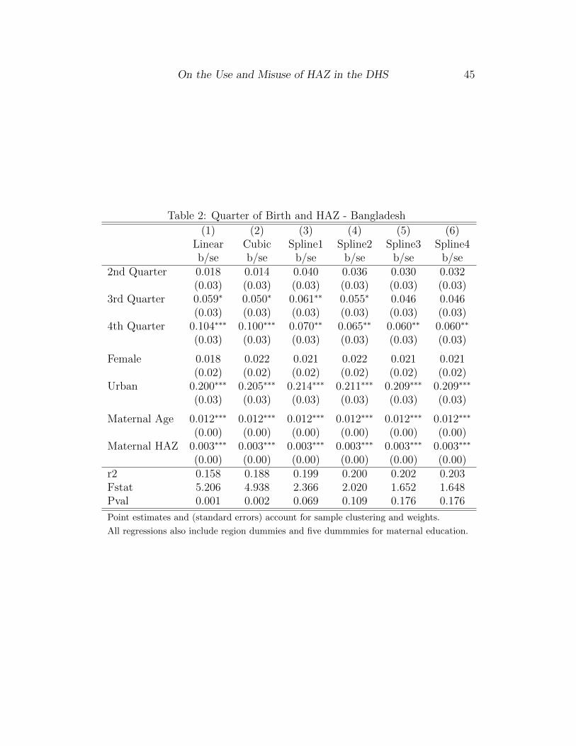
On the Use and Misuse of HAZ in the DHS 45
Table 2: Quarter of Birth and HAZ - Bangladesh
(1) (2) (3) (4) (5) (6)Linear Cubic Spline1 Spline2 Spline3 Spline4b/se b/se b/se b/se b/se b/se
2nd Quarter 0.018 0.014 0.040 0.036 0.030 0.032(0.03) (0.03) (0.03) (0.03) (0.03) (0.03)
3rd Quarter 0.059∗ 0.050∗ 0.061∗∗ 0.055∗ 0.046 0.046(0.03) (0.03) (0.03) (0.03) (0.03) (0.03)
4th Quarter 0.104∗∗∗ 0.100∗∗∗ 0.070∗∗ 0.065∗∗ 0.060∗∗ 0.060∗∗
(0.03) (0.03) (0.03) (0.03) (0.03) (0.03)
Female 0.018 0.022 0.021 0.022 0.021 0.021(0.02) (0.02) (0.02) (0.02) (0.02) (0.02)
Urban 0.200∗∗∗ 0.205∗∗∗ 0.214∗∗∗ 0.211∗∗∗ 0.209∗∗∗ 0.209∗∗∗
(0.03) (0.03) (0.03) (0.03) (0.03) (0.03)
Maternal Age 0.012∗∗∗ 0.012∗∗∗ 0.012∗∗∗ 0.012∗∗∗ 0.012∗∗∗ 0.012∗∗∗
(0.00) (0.00) (0.00) (0.00) (0.00) (0.00)Maternal HAZ 0.003∗∗∗ 0.003∗∗∗ 0.003∗∗∗ 0.003∗∗∗ 0.003∗∗∗ 0.003∗∗∗
(0.00) (0.00) (0.00) (0.00) (0.00) (0.00)r2 0.158 0.188 0.199 0.200 0.202 0.203Fstat 5.206 4.938 2.366 2.020 1.652 1.648Pval 0.001 0.002 0.069 0.109 0.176 0.176
Point estimates and (standard errors) account for sample clustering and weights.
All regressions also include region dummies and five dummmies for maternal education.

On the Use and Misuse of HAZ in the DHS 46
Tab
le3:
Log
GD
Pp
erca
pan
dH
AZ
-Z
imbab
we
(1)
(2)
(3)
(4)
(5)
(6)
(7)
UC
Lin
ear
Quad
Spline
NP
Spline-
QN
P-Q
b/s
eb/s
eb/s
eb/s
eb/s
eb/s
eb/s
elo
ggdp
1.12
2∗∗∗
0.85
3∗∗∗
0.47
6∗∗∗
0.30
1∗0.
277∗
0.41
1∗∗
0.38
7∗∗
(0.1
36)
(0.1
27)
(0.1
25)
(0.1
25)
(0.1
27)
(0.1
34)
(0.1
35)
bdat
e0.
001∗∗
0.00
0-0
.001∗
-0.0
01∗∗∗
-0.0
01∗∗∗
0.01
2∗0.
012∗
(0.0
00)
(0.0
00)
(0.0
00)
(0.0
00)
(0.0
00)
(0.0
05)
(0.0
05)
r20.
041
0.07
80.
126
0.13
40.
139
0.13
50.
139
Pva
lues
DH
S0.
000
0.00
00.
000
0.01
70.
029
0.00
20.
004
Coh
ort
Reg
ion
0.00
00.
000
0.00
50.
049
0.07
10.
012
0.01
9Surv
eyR
egio
n0.
002
0.00
00.
010
0.07
70.
115
0.04
70.
069
Reg
ion
Wild
0.55
60.
360
0.15
60.
140
0.16
40.
140
0.10
4C
ohor
tW
ild
0.38
80.
244
0.11
20.
280
0.24
80.
140
0.04
8
UC
isu
nco
nd
itio
nal
onag
e.L
inea
r,qu
ad
rati
c(Q
uad
)n
on
-para
met
ric
(NP
)re
fer
toage
contr
ols
.
Sp
lin
ere
fers
tocu
bic
spli
ne
wit
hin
tern
al
kn
ots
an
din
terc
epts
at
12,
24,
36,
an
d48
month
sof
age.
All
regr
essi
ons
also
incl
ud
ere
gio
nd
um
mie
s,ru
ral/
urb
an
an
dgen
der
du
mm
ies,
five
du
mm
ies
for
mat
ern
aled
uca
tion
an
dli
nea
rad
just
men
tsfo
rch
ild
bir
thd
ate
an
dm
ate
rnal
age
an
dH
AZ
.
Wei
ghte
du
sin
gre
-nor
mal
ized
sam
ple
pro
bab
ilit
yw
eights
.-Q
ind
icate
squ
ad
rati
cin
bir
thd
ate
incl
ud
ed.
Sta
nd
ard
Err
ors
inta
ble
acco
unt
for
wei
ghti
ng
an
dsa
mp
lin
gd
esig
n(D
HS
)
P-v
alu
esb
elow
com
par
etw
ocl
ust
erin
gle
vels
(Coh
ort
-an
dS
urv
ey-b
y-R
egio
n)
and
two
wil
dcl
ust
er-t
boot
stra
ps
(Reg
ion
an
dC
oh
ort
).

On the Use and Misuse of HAZ in the DHS 47
Table 4: Rejection Rates of Placebo GDP Effects
DHS Cluster BootstrapUnconditional 0.841 0.590 0.0387
Linear 0.780 0.656 0.0884
Quadratic 0.473 0.311 0.0663
Spline 0.341 0.213 0.0387
NP 0.390 0.273 0.0552
Statistical significance determined at 95 percent level.
DHS refers to standard errors accounting for survey design.
Cluster uses SEs clustered at region by cohort level.
Bootstrap from wild cluster-t bootstraps clustered at cohort level.

On the Use and Misuse of HAZ in the DHS 48
Table 5: Random Shocks Rejection Rates (.05 level)
Linear:
DHS 0.416
Cluster 0.0720
Spline:
DHS 0.292
Cluster 0.0780
FE
DHS 0.250
Cluster 0.0820
Clustered at region-by-cohort level

On the Use and Misuse of HAZ in the DHS 49
Table 6: Drought Shocks Rejection Rates by Age Control (.05 level)
1988 1992 1996 2000 2004Linear:
Beta (Linear) -0.00935 0.0119 0.0321 0.0181 0.00587(0.00165) (0.00168) (0.00162) (0.00167) (0.00169)
Survey Design 0.406 0.412 0.548 0.430 0.390(0.0220) (0.0220) (0.0223) (0.0222) (0.0218)
Region-Cohort 0.0700 0.0880 0.150 0.0980 0.0740(0.0114) (0.0127) (0.0160) (0.0133) (0.0117)
Spline:
Beta (Spline) -0.00793 0.00198 0.00715 0.00111 0.00464(0.00122) (0.00123) (0.00119) (0.00122) (0.00123)
Survey Design 0.282 0.262 0.260 0.268 0.274(0.0201) (0.0197) (0.0196) (0.0198) (0.0200)
Region-Cohort 0.0680 0.0620 0.0620 0.0560 0.0540(0.0113) (0.0108) (0.0108) (0.0103) (0.0101)
FE:
Beta (FE) 0.00142 0.000987 0.000435 0.00110 0.00140(0.00128) (0.00129) (0.00130) (0.00127) (0.00129)
Survey Design 0.276 0.272 0.254 0.268 0.280(0.0200) (0.0199) (0.0195) (0.0198) (0.0201)
Region-Cohort 0.0720 0.0800 0.0940 0.0700 0.0760(0.0116) (0.0121) (0.0131) (0.0114) (0.0119)
Region-Cohort denotes clustering level
Standard Errors of Mean in parentheses
Columns refer to year with additional shocks

On the Use and Misuse of HAZ in the DHS 50
A Sample Construction
All regression samples are constructed using the same selection procedures.First, I append all four survey rounds of each country and drop all obser-vations without height measurements, all children under the age of 1 monthand all observations where child birthdate is imputed (5 in Bangladesh, 21 inZimbabwe, and none in Peru). This leaves me with measurements on 22471children in Bangladesh, 14524 in Zimbabwe and 46357 in Peru. Of these,I drop 785 observations from Bangladesh, 1265 from Zimbabwe and 1243from Peru for having invalid measurements or measurements resulting in anHAZ score above 6 or below -6 standard deviations, which is the WHO defini-tion of the range of valid HAZ scores and is common practice in the literature(Borghi et al., 2006). Excluding children with missing covariate measurementsdrops an additional 335 observations in Bangladesh, 247 in Zimbabwe and909 in Peru. This leaves me with final sample sizes of: Bangladesh - 21351 ;Zimbabwe - 13012 ; and Peru - 44205 .
The DHS sampling method is partly unique to each survey but usu-ally follows a similar procedure in most years and countries. Geographicregions are defined, and the country is stratified by region and urban/ruralstatus. Clusters are chosen randomly from each strata, and households aresampled randomly (though with oversampling of some households) within clus-ter, though sampling is not uniform across time within strata16. Householdsare then assigned weights in order to make the weighted sample nationallyrepresentative, and these weights are normalized to sum to the sample size.All regressions in this work use re-normalized weights that sum to 1 withineach survey round, implicitly weighting each round equally. Using the originalDHS weights (which implicitly weights surveys by sample size), or using noweights at all, has no qualitative impact on the analyses presented.
16The fact that regions are surveyed at different times does lead to questions about theconsistency of point estimates from region fixed effect models. The issue is not addressedin this work. The Monte Carlo simulations in Section 5 give some evidence that any biasinduced by non-random sample timing across regions is likely to be of secondary concernin cases of region by birth year treatment assignment, but the effect may be problematic inother contexts