On the truthfulness of petal graphs for visualisation of data

Frode Eika Sandnes

Faculty of Technology, Art and DesignOslo and Akershus University College of Applied Sciences

AbstractA petal graph is an aesthetically attractive and applauded tool for visualisingparameter sets. For instance, petal graphs are often used by Norwegian policymakers and decision makers in higher education as the Ministry of Educationand Research relies on petal graphs in their reports. This study argues thatpetal graphs are prone to misinterpretation. It is challenging to interpret apetal graph in general, it is hard to compare two or more petal graphs andthis study demonstrates that the physical characteristics of petal graphs canbe incorrect in terms of the parameters on display. This study concludesthat the use of petal graphs should be abolished and that other visualisationtechniques to be used instead. Several alternatives are suggested.

1 IntroductionRadial visualisations are popular, but the choice of such visualisations are often basedon intuition rather than scientific arguments [4]. The literature on the effectiveness onradial visualisation techniques is limited [1] and has mostly focused on a limited set ofspecialised set of visualisation techniques — most of which are surveyed by Draper et al.[6]. Other visualisation techniques such as the petal plot remain unexplored and are thusthe focus of this study. A petal graph is a type of radial graph which exploits a flowermetaphor where groups of data are clustered into petals. For example, a dataset with fourclasses of data might be organised into four differently coloured petals. Each petal isconstructed from parameters represented by radial lines. The end points of these lines areconnected making up the petal area (see Figure 1).

A petal graph can be classified as a type of radar graph, also known as a star graph.Radar graphs are radial line plots of parameter sets that are popular for eye-catchingpresentations, but criticised for being hard to understand and providing little or no usefulinformation. Polar plots are also a type of radar graphs, but these usually represent datain some linear relationship, for instance measurements as a function of angle or time. Apolar plot could for instance represent the sensitivity of an omnidirectional microphone,or the load of a server during 24-hour cycles.

By inspecting a petal graph one easily notice individual parameters that stand out aslarge, strong areas and weak areas. Strong areas are represented by large petals and weakareas become small petals.

This paper was presented at the NIK-2012 conference; see http://www.nik.no/.

225

Figure 1: A petal graph (blomst) representing institutional parameters for HiOA (Osloand Akershus University College of Applied Sciences) from Database for Statistics onHigher Education.

Since 2009 the Ministry of Education and Research has published annual data in theform of interactive petal graphs on the website of the national Database for Statistics onHigher Education (DBH)1. One example of such a petal graph is shown in Figure 1. Thesegraphs are commonly used by senior administration staff and leaders in the Norwegianhigher education sector. The petal graphs are used to visualise snapshots of the state ofinstitutions such as education quality, research performance, internationalisation, regionalcontact, etc, and are intended to easily allow institutions to compare and benchmarktheir performance with other institutions. The Ministry of Education and Research isresponsible for the Norwegian education system and their data and reports therefore carrymuch weight, are assumed to be of high quality and are trusted. Their petal graphsfrequently appear in boardroom PowerPoint-presentation and written reports.

By viewing the petal graph in Figure 1 it is obvious that the institution-size petalis large and the regional contact petal is small, the research petal is quite small, theinternationalisation petal and education petals are medium sized. In other words, theoverall impression conveyed by the graph is a large institution with little regional contact.Apart from this impression the graph does not really say much else, besides the fact thatthe viewer can inspect the individual parameters.

Making comparisons is a key activity when viewers analyse charts. It is relativelyeasy to compare neighbouring objects, but it can be hard to compare the magnitude of

1http://dbh.nsd.uib.no/styringsdata/velg_blomst.action

226

two non-neighbouring parameters that are further apart — especially in radial graphs.Comparison is also more difficult when comparing parameters across two or more charts.The eyes have to move back and forth between the various plots and this process maylead to incorrect readings and misinterpretations. Another issue is the detection of changefor time-varying diagrams. However, time-varying diagrams are beyond the scope of thisstudy.

Figure 2: Misleading petal plot.

2 Physical properties of petal graphsFigure 2 illustrates a petal graph with four petals with the colours red, blue, green andyellow going in clockwise direction starting at the top right. This colour convention willbe used throughout this text. Which petal is the largest? It might be hard to assess, butsome observers would perhaps point out that the yellow and the blue petals are the largest— and for good reason, as these petals have the largest physical area. The yellow petal isthe largest with an area of 22.4 square units, the blue petal is the second largest with anarea of 19.7 square units, while the green petal is the second smallest with an area of 17.2square units and the red petal is the smallest with an area of 13.2 square units.

However, this is a misleading representation of the actual parameters as the twosmallest red and green petals have the largest parameters, and the two largest petals havethe smallest parameters. The red and the green both represent the same parameters 10,10, 3 and 3, while the yellow and the blue both represent the parameters 9, 9, 2 and 2.The area of the smallest petal with large parameters is only 59% of the area of the largestpetal with the small parameter set. The reason why identical parameters can give differentresults and larger parameters give a smaller area than small parameters is the sequence inwhich the parameters are presented. The impact of parameter sequence is explored in thefollowing sections.

227

Figure 3: A petal constructed from two triangles.

Imagine q parameters organised into w petals. The parameters in each petal Ci,i ∈ [1..w] are denoted by p1, p2, .. pN where N is the number of parameters in the petal.Each petal is constructed from N−1 triangles originating at the origin as shown in Figure3. The area of such a triangle is given by

A =12

absinz (1)

where a and b are the lengths of the two sides of the triangle leaving the origin and zis the angle of the triangle at the origin, given by

z =360q

(2)

It is assumed that the parameters are equally spaced around the circle. The area of theentire petal is thus given by

Atotal =12

N−1

∑i=1

pi pi+1sin(z) (3)

Since this discussion is concerned with the relative differences in area we can ignorethe constant factor sin(z)/2 and thus have the sum of parameter products given by:

T =N−1

∑i=1

pi pi+1 (4)

As indicated by the example above, the order of the parameters affects the size of thearea. If the parameters are organised such that pairs of large parameters are multiplied,that is, placed next to each other, it follows that the area will be large. However, if thelargest parameters are multiplied by the smallest parameters it follows that the area willbe smaller. Moreover, the first parameter p1 and the last parameter pN in the petal areonly a factor of one product, while all others are used twice. Therefore, whether thelargest or the smallest parameters are used in the first or last position will also affect theresults. A maximum area is obtained if the parameters are organised in decreasing orderand distributed with the largest parameters in the middle and the smallest at the ends, thatis at the first and the last position, or more formally:

Tmax : rN ,rN−2, ...,r3,r1,r2,r4, ...,rN−3,rN−1 (5)

228

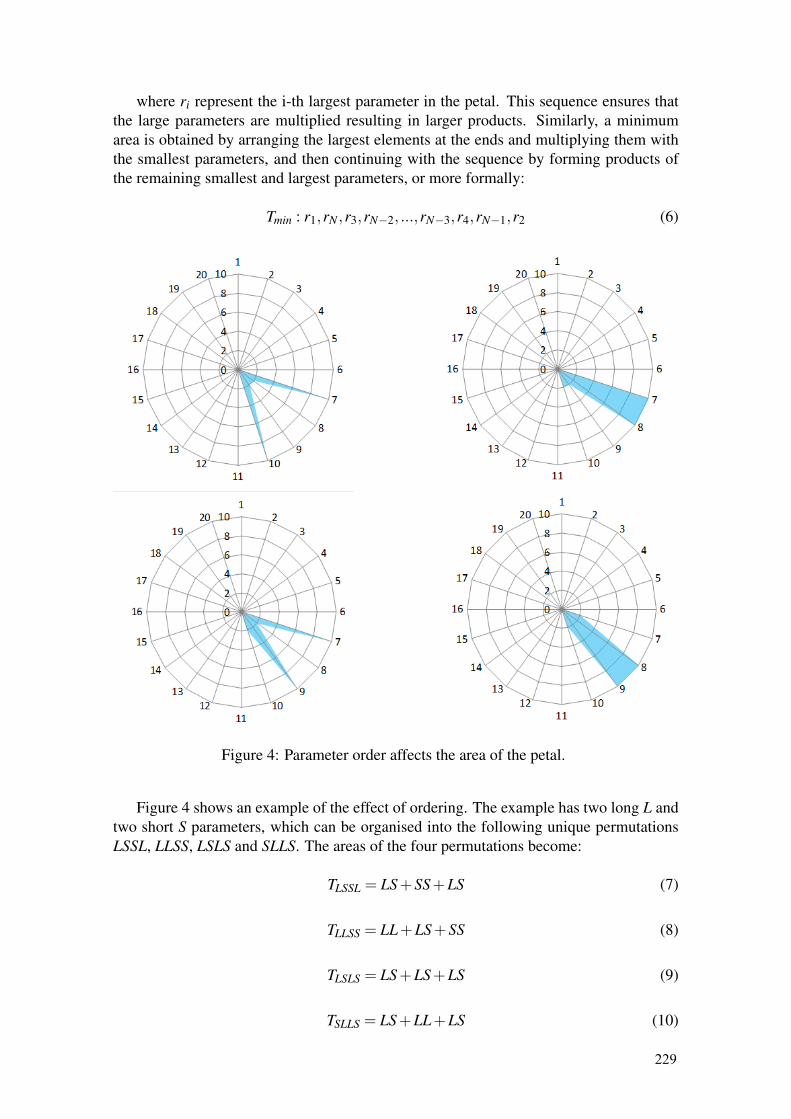
where ri represent the i-th largest parameter in the petal. This sequence ensures thatthe large parameters are multiplied resulting in larger products. Similarly, a minimumarea is obtained by arranging the largest elements at the ends and multiplying them withthe smallest parameters, and then continuing with the sequence by forming products ofthe remaining smallest and largest parameters, or more formally:

Tmin : r1,rN ,r3,rN−2, ...,rN−3,r4,rN−1,r2 (6)

Figure 4: Parameter order affects the area of the petal.

Figure 4 shows an example of the effect of ordering. The example has two long L andtwo short S parameters, which can be organised into the following unique permutationsLSSL, LLSS, LSLS and SLLS. The areas of the four permutations become:

TLSSL = LS +SS +LS (7)

TLLSS = LL+LS +SS (8)

TLSLS = LS +LS +LS (9)

TSLLS = LS +LL+LS (10)

229

An LS term can be removed from all sequences since the triangles are comparedrelatively, and when compared

TLSSL ≤ TLSLS ≤ TLLSS ≤ TSLLS (11)

since

SS +LS≤ LS +LS≤ LL+SS≤ LL+LS (12)

Clearly, the only scenario where the different sequences result in identical areas iswhen L = S, that is, when all the parameters are identical.

In conclusion, the physical characteristics of petal graphs are sensitive to thepresentation order of the parameters. This can lead to problems since parameters oftenhave no particular order and arbitrary presentation orders are chosen.

3 Perceptual properties of petal graphsThere is a vast literature on the perception of numbers, length and area [3, 5, 10,11]. Humans are better at comparing one-dimensional lengths than areas spanning twodimensions. When humans observe two dimensional shapes one is likely to look atone dimensional features. This is the reason bar graphs are effective. Petal graphsare constructed from single spikes or bars which are quite similar to traditional bars inbar charts. However, unlike the bar chart where all the bars start at the same line andare aligned in the same direction, the spikes in petal graphs are oriented in differentorientations. It is thus harder to compare the individual spikes. The ends of the spikesare connected with lines and the areas are filled in. These areas therefore become thedominant feature of petal graphs.

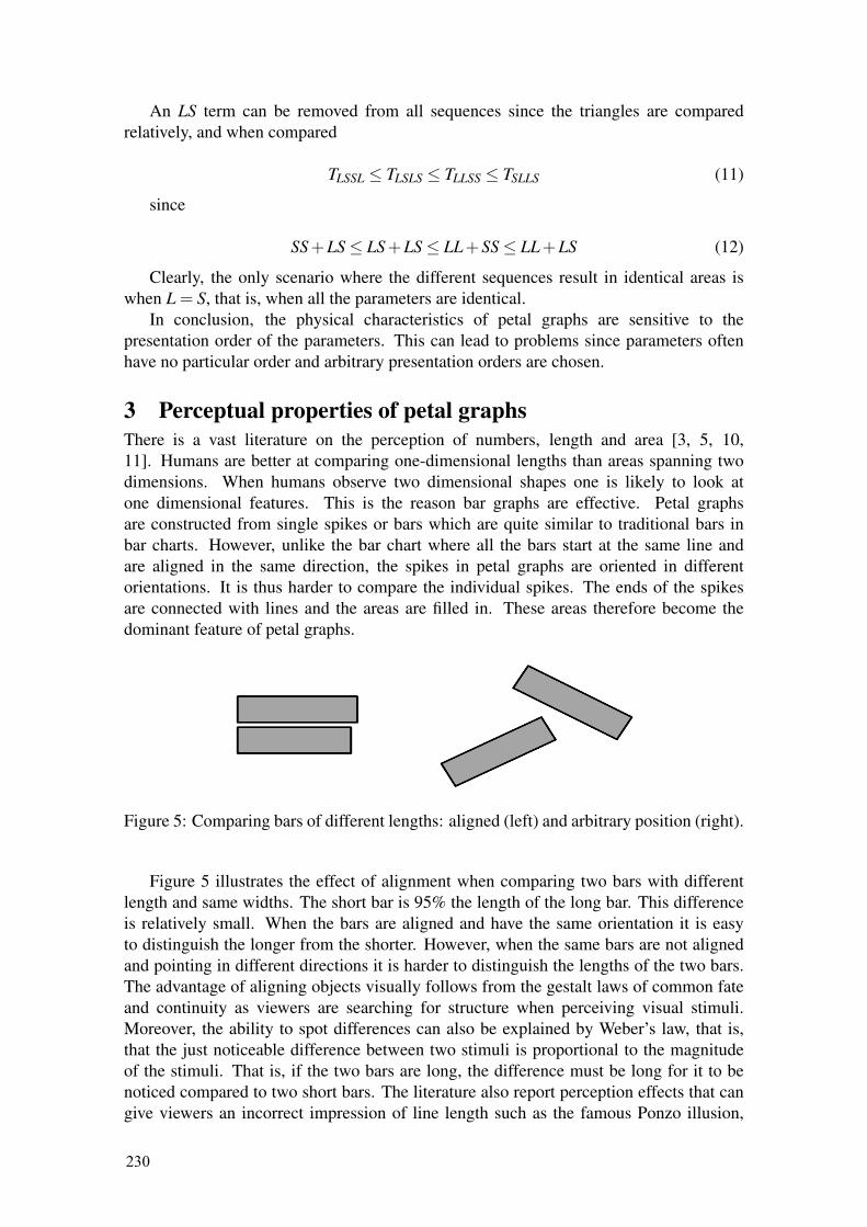
Figure 5: Comparing bars of different lengths: aligned (left) and arbitrary position (right).

Figure 5 illustrates the effect of alignment when comparing two bars with differentlength and same widths. The short bar is 95% the length of the long bar. This differenceis relatively small. When the bars are aligned and have the same orientation it is easyto distinguish the longer from the shorter. However, when the same bars are not alignedand pointing in different directions it is harder to distinguish the lengths of the two bars.The advantage of aligning objects visually follows from the gestalt laws of common fateand continuity as viewers are searching for structure when perceiving visual stimuli.Moreover, the ability to spot differences can also be explained by Weber’s law, that is,that the just noticeable difference between two stimuli is proportional to the magnitudeof the stimuli. That is, if the two bars are long, the difference must be long for it to benoticed compared to two short bars. The literature also report perception effects that cangive viewers an incorrect impression of line length such as the famous Ponzo illusion,

230

Muller-Lyer illusion and the horizontal-vertical illusion. Common to these illusions arethat the lines have different orientations.

Figure 6: Comparing areas. Left top and left bottom: original square, top right square:95% shorter sides, bottom right square: 95% less area.

Figure 6 illustrates how judging area is more difficult than judging length. The topleft diagram shows the original square and the top right a square where the both sizes arereduced to 95% of the sides of the original square. The right square is clearly smallerthan the left square, but the difference is less obvious than for the bar in Figure 5 wherethe length is much longer than the width. The bottom squares illustrates what happens ifthe reduction is measured in terms of area. The bottom left square is the original and thebottom right square has an area which is 95% of the original square. This square is moredifficult to distinguish from the original square, because the sides are more similar, thatis, 97.5% of the original. This is because the sides of the reduced square are equal to thesquare root of the 95% smaller area. Furthermore, if the squares are not aligned and havedifferent orientations the task of distinguishing the squares is even more difficult.

A general polygons is not square, but rather have a blob-like shape making thejudgment of dimensions and area more difficult. The disk is a polygon with infinitenumber of sides and Figure 7 illustrates that it is hard to assess small differences in diskdimensions. The right disk on the top row has a diameter 95% of the left disk. Althoughthe difference in size is perceivable it is not obvious. The bottom right disk has an area95% of the left disk, that is the diameter is just 97.5% of the left disk. It is much harderto assess the difference between these two shapes although they are aligned. Obviously,the orientation is irrelevant for the perception of disks. The effects of assessing the areasof disks versus squares has been addressed in the literature [5] and the results show thatobservers tend to underestimate the area of disks compared to squares.

The examples in Figures 2 and 4 where petals with larger parameters appear smallerthan petals with smaller parameters are consistent with the classic study of perception ofshape area by Smith [11]. Smith constructed 30 images with shapes of identical areasconstructed from squares. A perception study showed that the subjects classified long andnarrow shapes as having less area than the compact and dense shapes. In the examples inFigures 2 and 4 the large parameter petals have a thinner V-like shape while the smallerparameter petals have a more bulky condensed shape thus appearing to have larger area.

231

Figure 7: Comparing the differences between disks with different areas. Top: the diameterof the smaller (right) is 95% of the larger (left), bottom: the area of the smaller (right) is95% of the larger (left).

Figure 8: Two shapes with identical area (34 squares) inspired by Smith [11]. The longand thin shape (left) is perceived to have a smaller area than the compact and dense shapes(right).

Figure 8 illustrates the different perception of area according to Smith’s study.

4 Alternative visualisation techniquesAs implied in the previous sections the petal graphs embody certain characteristicswhich render them unsuitable for the visualisation of parameters. Another visualisationtechnique that is used for the same purposes are sunburst diagrams, also known as radialbar diagrams and polar area diagrams [6]. A sunburst diagram is a radial diagram withbar graphs, or rays, originating from one central point and dispersing out in all directions.The length of the ray suggests the magnitude of its parameter. Moreover, the sunburstrays spread out in the shape of triangles. Thus, the larger the bar, the wider one endis. Sunburst graphs are for instance used in the European U-map initiative2 hosted bythe Center for Higher Education Policy Studies (CHEPS) which purpose is to classifyEuropean higher education institutions. An example of a u-map sunburst diagram isshown in Figure 9. Sunburst diagrams are also used for the visualisation of documentcontents [2] and multivariate analysis [9].

Figure 10 illustrates the visual difference between two sunburst beams as used insunburst graphs. It is relatively easy to spot that there is a difference between the twobeams on the right, and it is even easier to spot the difference when these beams are

2http://www.u-map.eu/

232

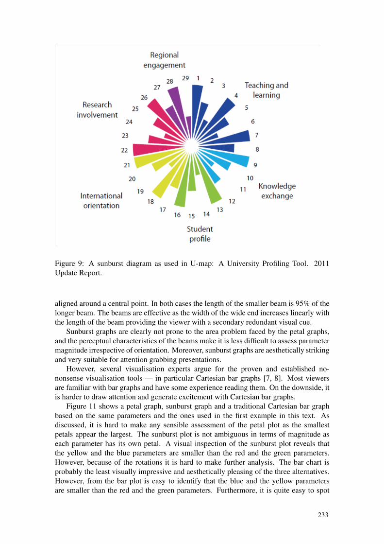
Figure 9: A sunburst diagram as used in U-map: A University Profiling Tool. 2011Update Report.

aligned around a central point. In both cases the length of the smaller beam is 95% of thelonger beam. The beams are effective as the width of the wide end increases linearly withthe length of the beam providing the viewer with a secondary redundant visual cue.

Sunburst graphs are clearly not prone to the area problem faced by the petal graphs,and the perceptual characteristics of the beams make it is less difficult to assess parametermagnitude irrespective of orientation. Moreover, sunburst graphs are aesthetically strikingand very suitable for attention grabbing presentations.

However, several visualisation experts argue for the proven and established no-nonsense visualisation tools — in particular Cartesian bar graphs [7, 8]. Most viewersare familiar with bar graphs and have some experience reading them. On the downside, itis harder to draw attention and generate excitement with Cartesian bar graphs.

Figure 11 shows a petal graph, sunburst graph and a traditional Cartesian bar graphbased on the same parameters and the ones used in the first example in this text. Asdiscussed, it is hard to make any sensible assessment of the petal plot as the smallestpetals appear the largest. The sunburst plot is not ambiguous in terms of magnitude aseach parameter has its own petal. A visual inspection of the sunburst plot reveals thatthe yellow and the blue parameters are smaller than the red and the green parameters.However, because of the rotations it is hard to make further analysis. The bar chart isprobably the least visually impressive and aesthetically pleasing of the three alternatives.However, from the bar plot is easy to identify that the blue and the yellow parametersare smaller than the red and the green parameters. Furthermore, it is quite easy to spot

233

Figure 10: Assessing the difference between sunburst beams. Arbitrary positioned (left)and radiating from origin (right).

Figure 11: Comparison of a petal graph, a sunburst graph and a traditional Cartesian bargraph using the same set of parameters as in Figure 2.

that these data within the two groups have the same magnitude. These observations areconsistent with the results reported in the literature. User studies have uncovered thatfor certain radial graph types and their Cartesian counterparts the Cartesian plots leads tobetter results while the radial plots are more effective as small thumbnails [1]. It has alsobeen pointed out that it is easier to remember positions on a radial graphs, compared toCartesian graphs [1] and that it is easier to remember outer or border cells than inner andnon border cells [4]. Users also tend to need shorter time deciphering Cartesian plots thanradial plots and that there is a positive effect of reading directions in Cartesian plots [4].

5 ConclusionsAlthough petal graphs are visually striking and attractive for making striking presentationsthis study argues that petal visualisation are prone to misinterpretation. The sequenceorder used is usually arbitrary and this study has shown that the parameter ordering affectsthe physical area of the petals. Moreover, the problems with petal graphs are supportedby classic studies on perception of area where long and thin shapes are perceived assmaller than more concentrated and bulky shapes even when these shapes have similararea. The petal graph also suffers from the same problems as other radial visualisationapproaches as reported in the literature. In particular, it is hard to compare the relativemagnitude of each parameter, and it is difficult to compare parameters across differentplots. It is recommended that petal plots are replaced by sunburst diagrams or preferablytraditional Cartesian bar graphs despite the fact that the latter are less visually exciting.This conclusion echoes the recommendation posed in the literature, that is, not to chooseradial visualisation approaches unless there is a very good reason to do so [4]. Moreover,

234

trusted organisations with a strong impact on society such as the Ministry of Educationand Research should take special care to ensure quality in their official visualisations.

6 AcknowledgementI would like to acknowledge Simen Hagen who started a study on the effectiveness ofradar graph visualisations before he passed away.

References[1] Burch, M., Bott, F., Beck, F. and Diehl, S. Cartesian vs. Radial — A Comparative

Evaluation of Two Visualization Tools. Lecture Notes in Computer Science 5358,151-160 (2008).

[2] Collins, C. DocuBurst: Radial Space-Filling Visualization of DocumentContent. Technical Report KMDI-TR-2007-1, University of Toronto (2007),http://www.kmdi.utoronto.ca/files/publications/2010/KMDI-TR-2007-1.pdf.

[3] Dehaene, S., Izard, V., Spelke, E. and Pica, P. Log or linear? Distinct intuitionsof the number scale in Western and Amazonian indigene cultures. Science 320,1217-1220 (2008).

[4] Diehl, S., Beck, F. and Burch, M. Uncovering Strengths and Weaknesses of RadialVisualizations—an Empirical Approach. IEEE Transactions on Visualization andComputer Graphics 16 (6), 395-942 (2010).

[5] Di Maio V. and Lansky P. Area perception in simple geometrical figures. Perceptionand Motor Skills 71 (2), 459-525 (1990).

[6] Draper, G.M., Livnat, Y. and Riesenfeld, R.F. A Survey of Radial Methodsfor Information Visualization. IEEE Transactions on Visualization and ComputerGraphics 15 (5), 759-776 (2009).

[7] Few, S. Show Me the Numbers: Designing Tables and Graphs to Enlighten.Analytics Press , (2004).

[8] Few, S. Information Dashboard Design: The Effective Visual Communication ofData. O’Reilly Media, (2006).

[9] Liu, R.Y., Parelius, J.M. and Singh, K. Multivariate analysis by data depth:Descriptive statistics, graphics and inference. Annals of Statistics 27 (3), 783-840(1999).

[10] Mates J., Di Maio V., Lansky P. A model of the perception of area. Spatial Vision 6(2), 101-117 (2009).

[11] Smith, J. The effects of figurai shape on the perception of area. Attention, Perception,& Psychophysics 5 (1), 49-52 (1969).

235