1

DEPARTMENT OF ECONOMICS

ISSN 1441-5429

DISCUSSION PAPER 31/12

On the Time Inconsistency of Optimal Monetary and

Fiscal Policies With Many Consumer Goods

Begoña Dominguez

* and Pedro Gomis-Porqueras

†

Abstract This paper studies optimal monetary and fiscal policies in an economy à la Lucas and

Stokey (1983) and Lagos and Wright (2005) with multiple cash and credit goods. We

show that optimal policies are in general time inconsistent due to insufficient number of

instruments to influence future government decisions. There are two important cases where

time consistency can be restored. First, if taxes in the decentralized anonymous markets

are not available, the multipliers on the decentralization constraints can be utilized as

additional instruments to ensure time consistency. Second, if taxes in decentralized markets

are available, time consistency arises when the different cash goods satisfy the conditions

necessary for optimal uniform taxation.

JEL Codes: C70, E40, E61, E62, H21.

Keywords: optimal policy; time consistency; taxation; money; inflation; search.

*Corresponding author: Begoña Dominguez School of Economics, The University of Queensland, Colin Clark

Building(39), St Lucia, Brisbane, Qld 4072, Australia. E-mail: b.dominguez@uq.edu.au

†Department of Economics, Monash University, Caulfield Campus, Room H4.31, Caulfield East, Vic 3145,

Australia. E-mail: pedro.gomis@monash.edu

© 2012 Begoña Dominguez and Pedro Gomis-Porqueras

All rights reserved. No part of this paper may be reproduced in any form, or stored in a retrieval system, without the prior written

permission of the author.

1 Introduction

Can governments induce commitment to optimal monetary and fiscal policies? In an environment

where fiat money is essential, this paper examines this question and demonstrates that when

there are multiple government policy decisions per period affecting nominal variables, optimal

monetary and fiscal policies are in general time inconsistent.

This paper studies optimal fiscal and monetary policies in an environment that blends the

shopper-worker structure of Lucas and Stokey (1983) with the sequential nature of trade, lack

of enforcement and informational frictions of Lagos and Wright (2005). In every period agents

trade in two different markets. First they trade in a decentralized anonymous market (DM)

where the only incentive compatible form of payment is fiat money.1,2 Then agents trade in

a centralized market (CM) where any form of payment is possible. Agents consume positive

amounts of several consumer goods in both markets. These DM and CM goods are the same in

terms of their product characteristics, but they are intrinsically different as they are traded in

different locations and require different forms of payment.

In order to finance an exogenous government spending, the benevolent government chooses a

general tax rate on all CM goods, a specific tax rate on each CM good (other than the benchmark

CM good 1), nominal interest rates that affect all DM goods, a specific tax rate on each DM

good (other than than the benchmark DM good 1), the initial level of prices, and the issues of

nominal and real government bonds. Real bonds can be indexed to each CM good. However, as

in Lucas and Stokey (1983), bonds indexed to DM goods are not allowed as that would not be

consistent with having DM goods bought at decentralized markets where agents are anonymous.3

This is a crucial assumption for the results of the paper as well as for the existence of money.

Our main findings are as follows. We show that optimal policies are in general time inconsis-

tent because governments do not have a sufficient number of instruments to influence all future

government decisions. There are two important cases where time consistency can be restored.

1Kocherlakota (1998) laid out the critical frictions for fiat money to be essential. He showed that if any of thefollowing elements in the economic environment are absent: (i) recordkeeping over individual trading histories(“memory”), (ii) public communication of histories and (iii) sufficient enforcement (or punishment), then creditbetween buyer and seller is not incentive compatible so money is essential. The search literature uses the term“anonymity” to encompass these three frictions.

2 We rule out bonds as a medium of exchange. For that to hold in equilibrium, the literature argues that bondsmust have some iliquidity relative to fiat money. Wallace (1983) and Aiyagari, Wallace and Wright (1996) arguethat bonds are illiquid because of legal restrictions that prohibit the issuing of bonds of small denomination. Onthe other hand, Li, Rocheteau and Weill (2011) emphasize informational asymmetries between assets that affectrecognizability properties of fiat money and bonds determining the liquidity of assets as an equilibrium outcomeendogenously.

3In an economy with one cash good and one credit good, Lucas and Stokey (1983) write: “If such securitieswere available, however, they could be used by agents to circumvent the use of currency altogether, convertingthe system directly into the two-good barter economy ... This would conflict with our interpretation of cashgoods as being anonymously purchased in spot markets only. To maintain the monetary interpretation of themodel, then, direct claims to cash goods in “real” terms will be ruled out.”

2

First, if taxes in the decentralized anonymous markets are not available, the multipliers on the

decentralization constraints can be used as additional instruments to ensure time consistency.

Second, if taxes in decentralized markets are available, time consistency arises when the differ-

ent decentralized market goods satisfy the conditions necessary for optimal uniform taxation.

Therefore, the frictions that make money essential, anonymity and lack of enforcement, which

are important for the feasibility of taxation in DM, are then also relevant for time consistency.

This is consistent with Wallace (2001) who points out that different approaches of modelling

money have important implications for other parts of the model. In our paper, informational

frictions that make fiat money essential also shape the debt and tax instruments available and

the sustainability of the resulting optimal fiscal and monetary policies.

This paper builds on the existing literature on the time consistency of optimal monetary and

fiscal policies.4 Since the seminal work of Calvo (1978), the severity of the time inconsistency

problem of monetary and fiscal policies has been widely recognized and studied. Lucas and

Stokey (1983) show that the incentives to inflate away the initial stock of nominal bonds and

money are so severe that optimal monetary and fiscal policies cannot be made time consistent.

Recently, two papers have proposed solutions to this classic problem in public finance. Alvarez,

Kehoe and Neumeyer (2004) find that optimal monetary and fiscal policies are time consistent

when the Friedman rule is optimal, as their monetary economy becomes isomorphic to a real

economy. Persson, Persson and Svensson (2006) have demonstrated that time consistency in

optimal monetary and fiscal policies can be achieved independently of the optimality of the

Friedman rule whenever surprised inflation imposes some direct costs to agents.

This paper relates to both articles. As in Persson et al. (2006), we assume that consumption

in decentralized markets takes place before centralized market trades. This timing assumption

implies that surprise inflation has a direct cost in the economy and the optimal initial level of

prices is finite. However, relative to Persson et al. (2006), our environment has multiple goods

that require fiat money to settle trade. Thus optimal policies cannot be made time consistent

with just one nominal bond. In contrast to Alvarez et al. (2004), in our environment the

Friedman rule is not always optimal. Nevertheless, even when the Friedman rule is optimal,

future fiscal choices in decentralized markets cannot be influenced by current governments. This

implies that optimal monetary and fiscal policies are time inconsistent even when the Friedman

rule is optimal.

This paper justifies and complements the work of Martın (2011) who considers a search

theoretic model of fiat money where agents face some limited commitment in some markets and

where the government can not commit to future policies. Martın (2011) studies time-consistent

Markov policies and finds that when net nominal government obligations are positive, there

4Persson et al. (2006) provide a comprehensive review of the literature.

3

exists a unique steady state with positive net nominal government obligations, which is stable

and time-consistent. For any initial level of debt, the welfare loss due to lack of commitment is

small. Within the framework, Martın (2012a) studies the determination of government policy

when aggregate shocks (expenditure and labor productivity) are present while considering various

trading protocols in decentralized markets. The author finds that fiscal and monetary policies

are distortionary, but long-run policy is not afflicted by time-consistency problems when different

trading protocols are considered.5

As in Martın (2011) and (2012a), this paper tries to improve our understanding of the inherent

links between fiscal and monetary policies in the absence of commitment both by governments

and by agents in some markets. By considering alternative approaches to modeling fiat money

that emphasize different frictions in the economic environment, we are able to determine the

robustness of the policy prescriptions prescribed by the previous literature.

The structure of the rest of the paper is as follows. Section 2 describes our model economy.

Section 3 characterizes optimal fiscal and monetary policies with commitment. Section 4 studies

the time consistency of the optimal policy. Section 5 concludes.

2 The environment

We consider an economy that incorporates elements of Lucas and Stokey (1983) and various

ingredients of search-theoretic models of money. In particular, we consider the large household

framework of Shi (1997) and the sequential nature of trade and informational frictions of Lagos

and Wright (2005) making a medium of exchange essential.

Time is discrete and indexed by t. The economy is comprised by a continuum of households

that live forever and have a common discount factor β ∈ (0, 1) between time periods. Within

each household, agents belong to a large family of measure one. Every period is comprised

of two sub-periods or stages, day and night, which differ in terms of the enforcement and the

informational frictions that agents face.

In the first stage (day), households trade in a decentralized market (DM). This market is

characterized by anonymous trades, lack of enforcement, no record-keeping services and by a

lack of double coincidence of wants. Given these assumptions, the only feasible trade in DM is

the exchange of goods for fiat money.6 A fraction κ ∈ (0, 1) of household members are potential

buyers (who can buy but not sell) and a fraction (1− κ) are potential sellers (who can sell but

not buy). With probability σ ∈ (0, 1), agents (buyers and sellers) of all families are randomly

5Martın (2012b) considers a similar environment and evaluates the implied time-consistent Markov policies inexplaining U.S. wartime. The author finds that during the period under analysis there were strong incentives toinflate as the government was faced by an increased stock of debt.

6Since there are no record keeping services, bonds cannot be used as a medium of exchange in DM.

4

assigned to different identical locations in DM. If agents are not assigned to any location, they

cannot trade in DM for that period. Otherwise, buyers and sellers of each family are sent to

different locations. Thus, as in Shi (1997), members of the same family cannot trade with each

other. The matching technology is such that the measure of buyers and sellers is the same across

all locations as in Lucas and Prescott (1974). In order to be closest to the cash and credit good

economy of Lucas and Stokey (1983), we assume that the trading protocol in DM is competitive

pricing. Once trades take place, all members of the household share the proceeds of the DM

trade before moving into the next market.

In the second stage (night), households trade in a centralized market (CM). In this market,

all members of the family can produce and consume CM goods as well as adjust their portfolio

by rebalancing their money and (real and nominal) bond holdings. In this market there are no

informational frictions nor lack of double coincidence of wants thus a medium of exchange is not

essential.

2.1 Many Consumer Goods

In this environment we consider multiple consumer goods both in CM and DM. More specifically,

individuals want to consume I>1 distinct consumption goods in CM, denoted by the vector Xt =

(X1,t, ..., XI,t), and I>1 distinct consumption goods in DM, denoted by xt = (x1,t, ..., xI,t). The

I goods in CM and DM are not perfectly substitutable within each sub-market and individuals

require positive amounts of consumption of each good.

The key difference between CM and DM goods is the market in which they are purchased

and therefore the available payments methods to settle trade. The first vector of CM goods, Xt,

is purchased by any means of payment available in the economy. On the other hand, the vector

of DM goods, xt, can only be purchased with fiat money given the informational frictions in that

market. We follow Lucas and Stokey (1983) in assuming that CM and DM goods cannot be

singled out through observable “product” characteristics. However, the market, in which they

are purchased, makes consumption Xi,t different from consumption xi,t. Moreover, these goods

may have a different income elasticity of demand and may yield different utilities.7

We allow governments to issue bonds indexed to the CM good i, for all i = 1, .., I. However,

as also argued in Lucas and Stokey (1983), we do not allow for bonds indexed to DM goods as

that would conflict with having DM goods been bought at decentralized markets (where agents

are anonymous and lack enforcement) and would make money non essential. As mentioned, this

is a crucial assumption for the results of the paper as well as for the existence of money.

7An example of what we have in mind is the following: a hot-dog sold at a stadium stand during a soccer matchis a DM good and a hot-dog sold at the corner shop owned by a neighbour friend is a CM good. Both underlyingconsumption goods are identical, but they are sold at different markets with different payment methods. Thismakes both products in fact different and with a likely different demand elasticity.

5

2.2 Preferences and Technologies

At any date t, households have preferences over all of the I DM consumption goods (xt =

(x1,t, ..., xI,t)), total effort exerted to produce all of the DM goods (lt =∑I

i=1 li,t), all of the I

CM consumption goods (Xt = (X1,t, ..., XI,t)) and total effort exerted to produce all of the CM

goods (Lt =∑I

i=1 Li,t). These are given by:

E0

∞∑t=0

βt[u(xt)− h(lt) + U(Xt)−H(Lt)]. (1)

The instantaneous utility functions u(·), U(·), h(·) and H(·) are all strictly increasing and three

times continuously differentiable. The functions u(·) and U(·) are strictly concave. For all i,

we assume that uxi = ∞ whenever xi = 0 and, equivalently, UXi = ∞ whenever Xi = 0.

Throughout the rest of the paper, subscript xi denotes the derivative of the function with respect

to xi. To simplify the analysis, both u(·) and U(·) are assumed to be additively separable, so

that uxi,xj = UXi,Xj = 0 for i 6= j, with i, j ∈ 1, ..., I.8 It is important to note that the functions

u(·) and U(·) do not have to satisfy homotheticity, or have the same specific form. We further

assume that the functions h(·) and H(·) are strictly convex and satisfy h(0) = H(0) = 0 and

hl(1) = HL(1) =∞.9

In DM all consumption goods are produced according to a constant returns technology f ,

where labor is the only input and one unit of labor yields one unit of output, f(li,t) = li,t. Recall

that only a fraction of the family can actually produce these goods. On the other hand, in the

CM, all members of the family can produce goods. Agents have also access to a linear production

technology F that can transform labor into final goods so that F (Li,t) = Li,t.

2.3 Solving the Agent’s Problem

Next we solve the agent’s problem recursively. Thus, we first solve the second stage (CM) problem

taking the actions of the first stage as given. We then solve the first stage (DM) problem.

2.3.1 The Second Stage Problem

After trades take place in DM, agents enter the next submarket CM before the end of the period.

Since in this market agents can both produce and consume goods, there is no double coincidence

of wants problem and thus a medium of exchange is not essential. Moreover, since there are no

informational frictions, agents can settle their trades with any asset or CM goods.

8Our results can be generalized to non-separable instantaneous utility functions.9Given our assumptions on the trading opportunities, we do not require linearity in the disutility of labor to

guarantee degeneracy of asset holdings across households.

6

An agent arrives at the beginning of CM with a portfolio of fiat money holdings, nominal

and real government bonds, and with a tax liability TDMt . This asset position and tax liability

reflect the trades in the previous DM. Agents can rebalance their portfolio and have to pay any

tax liabilities arising from CM trade before moving into the next DM.10

We assume that initial conditions are identical for all agents within the family and across all

different households which we later show is consistent with equilibrium. In what follows, let bNt+1,s

andbit+1,s

Ii=1

respectively denote the nominal and real bonds, indexed to the CM consumption

good i, issued at the end of period t with maturity s = t + 1, ...,∞. For nominal bonds, we

denote by qNt,s the price of one dollar in period s in units of dollars in period t. Similarly, for

real bonds, qit,s denotes the price of the CM good i in period s in units of the CM consumption

good i in period t. We normalize qNt,t = 1 and qit,t = (1 + τCt )(1 + τXi,t), where τCt is a general

tax rate on all CM goods and τXi,t represents a specific tax rate for good i. From now on we use

the consumption good 1 in CM as the benchmark good and set τX1,t ≡ 0.11 As is standard in

the literature, we assume that bond payments are not taxable and that governments honor their

debt payments. The agent’s budget constraint in CM is then given by

I∑i=1

Pt(1 + τCt )(1 + τXi,t)Xi,t +mNt+1 +

∞∑s=t+1

qNt,sbNt+1,s + Pt

∞∑s=t+1

I∑i=1

qit,sbit+1,s =

PtwtLt − TDMt +mNt +

∞∑s=t

qNt,sbNt,s + Pt

∞∑s=t

I∑i=1

qit,sbit,s, (2)

where Pt is the nominal price index of CM goods (Xt), mNt represents fiat money holdings at

time t, bNt denotes the vector of nominal bonds with different maturities, and bt is the matrix of

real bonds for different CM goods and maturities.

The problem of the representative agent consists of maximizing her welfare while taking

prices, taxes, initial conditions, and the distribution of money holdings of other agents as given

which is summarized by

W (mNt , b

Nt , bt) = max

Xt,Lt,mNt+1,bNt+1,bt+1

U(Xt)−H(Lt) + βV (mNt+1, b

Nt+1, bt+1) subject to (2),

where W (·) denotes an agent’s value function at the beginning of the period-t in CM and V (·)represents the family’s value function at the beginning of the period-t+1 in DM.

Substituting Lt from the budget constraint into the objective, the first-order conditions with

10For sake of generality, we first allow for taxation in the DM market. In what follows it does not matter forthe results whether DM taxes are paid in CM or in DM.

11It is easy to see that this tax structure is equivalent to one tax rate per CM good, which for the one goodcase it is also equivalent to a labor tax rate.

7

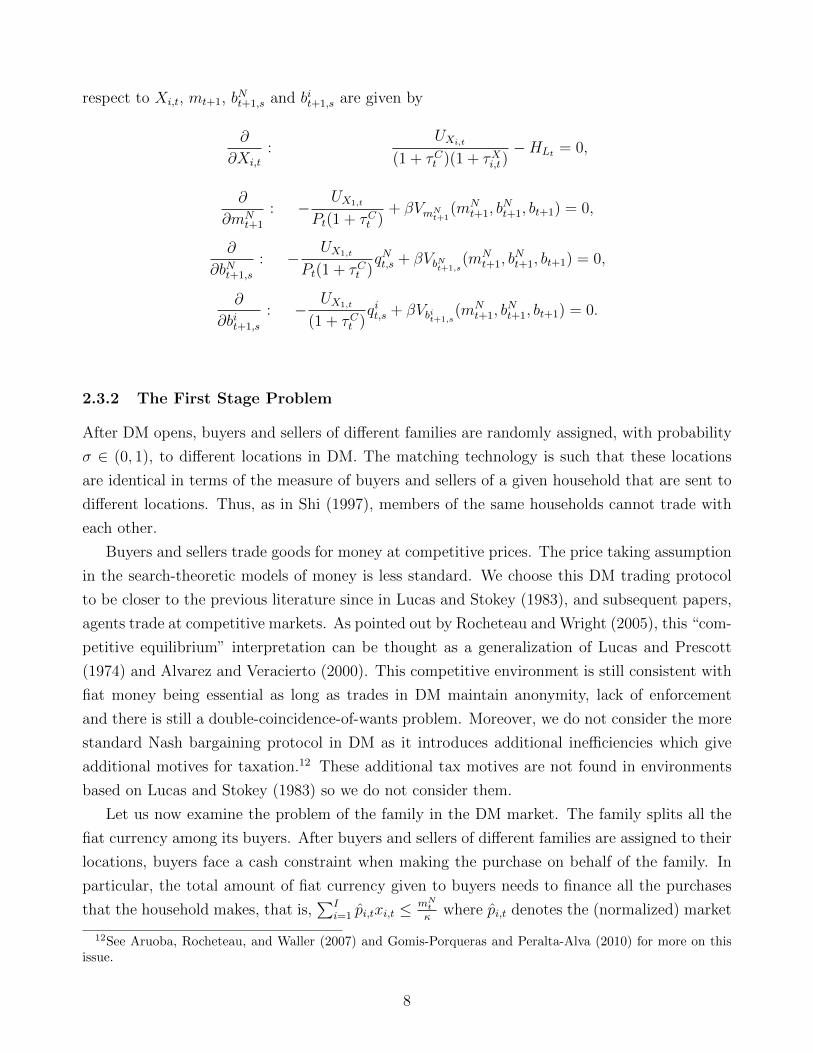
respect to Xi,t, mt+1, bNt+1,s and bit+1,s are given by

∂

∂Xi,t

:UXi,t

(1 + τCt )(1 + τXi,t)−HLt = 0,

∂

∂mNt+1

: −UX1,t

Pt(1 + τCt )+ βVmNt+1

(mNt+1, b

Nt+1, bt+1) = 0,

∂

∂bNt+1,s

: −UX1,t

Pt(1 + τCt )qNt,s + βVbNt+1,s

(mNt+1, b

Nt+1, bt+1) = 0,

∂

∂bit+1,s

: −UX1,t

(1 + τCt )qit,s + βVbit+1,s

(mNt+1, b

Nt+1, bt+1) = 0.

2.3.2 The First Stage Problem

After DM opens, buyers and sellers of different families are randomly assigned, with probability

σ ∈ (0, 1), to different locations in DM. The matching technology is such that these locations

are identical in terms of the measure of buyers and sellers of a given household that are sent to

different locations. Thus, as in Shi (1997), members of the same households cannot trade with

each other.

Buyers and sellers trade goods for money at competitive prices. The price taking assumption

in the search-theoretic models of money is less standard. We choose this DM trading protocol

to be closer to the previous literature since in Lucas and Stokey (1983), and subsequent papers,

agents trade at competitive markets. As pointed out by Rocheteau and Wright (2005), this “com-

petitive equilibrium” interpretation can be thought as a generalization of Lucas and Prescott

(1974) and Alvarez and Veracierto (2000). This competitive environment is still consistent with

fiat money being essential as long as trades in DM maintain anonymity, lack of enforcement

and there is still a double-coincidence-of-wants problem. Moreover, we do not consider the more

standard Nash bargaining protocol in DM as it introduces additional inefficiencies which give

additional motives for taxation.12 These additional tax motives are not found in environments

based on Lucas and Stokey (1983) so we do not consider them.

Let us now examine the problem of the family in the DM market. The family splits all the

fiat currency among its buyers. After buyers and sellers of different families are assigned to their

locations, buyers face a cash constraint when making the purchase on behalf of the family. In

particular, the total amount of fiat currency given to buyers needs to finance all the purchases

that the household makes, that is,∑I

i=1 pi,txi,t ≤mNtκ

where pi,t denotes the (normalized) market

12See Aruoba, Rocheteau, and Waller (2007) and Gomis-Porqueras and Peralta-Alva (2010) for more on thisissue.

8

price of good xi,t. The problem of the household then can be written as follows

V (mNt , b

Nt , bt) = max

xi,t,li,t

σ

[κχxu(xt)− (1− κ)χlh

(I∑i=1

li,t

)+ εt

(mNt

κ−

I∑i=1

pi,txi,t

)]+

W

(mNt − σκ

I∑i=1

pi,txi,t + σ(1− κ)I∑i=1

pi,t(1− τSi,t)li,t, bNt , bt

),

(3)

where εt denotes the Lagrange multiplier on the cash constraint, τSi,t is a sales tax rate on DM

good i,∑I

i=1 pi,t(1 − τSi,t)li,t is the total amount of cash (net of sales taxes) that sellers from

the household receive to compensate for their exerted effort, χx < 1 and χl > 1 represent the

loss in utility due to the random assignment process.13 We again use good 1 as the benchmark

good and set τS1,t ≡ 0. Note that the inflation tax affects all DM goods and therefore the same

number of tax instruments are now available in both CM and DM.14 As in Shi (1997), in this

environment members of the same household share all of the proceeds as well as the costs of

trading in DM before they trade in the next CM.

The first order conditions for consumption and labor are respectively

∂

∂xi,t: σκ χxuxi,t − σεtpi,t − σκpi,t

UX1,t

Pt(1 + τCt )= 0,

∂

∂li,t: −σ(1− κ) χl hlt + σ(1− κ)pi,t(1− τSi,t)

UX1,t

Pt(1 + τCt )= 0.

Solving for εt in the first equation, then the resulting envelope conditions are given by

VmNt = σεtκ

+UX1,t

Pt(1 + τCt )= σ χx

uxi,tpi,t

+ (1− σ)UX1,t

Pt(1 + τCt ),

VbNt,s =UX1,t

Pt(1 + τCt )qNt,s,

Vbt,s =UX1,t

(1 + τCt )qit,s.

2.4 Government

We consider a benevolent government that must finance the government spending, Gt in every

period, through distortionary taxes and by issuing bonds and fiat money. The real value of all

13In Shi (1997) the household can choose the search intensity which is costly in utility terms.14If we allow for a rate τS1,t different from 0, we have multiple tax structures that decentralize a competitive

equilibrium.

9

issues at every period is assumed to be bounded above by a sufficiently large constant in order

to avoid Ponzi schemes. The corresponding government budget constraint is given by

I∑i=1

PtτCt (1 + τXi,t)Xi,t +

I∑i=2

PtτXi,tXi,t + TDMt +mN

t+1 +∞∑

s=t+1

qNt,sbNt+1,s + Pt

∞∑s=t+1

I∑i=1

qit,sbit+1,s ≥

PtGt +mNt +

∞∑s=t

qNt,sbNt,s + Pt

∞∑s=t

I∑i=1

qit,sbit,s;

where TDMt = σκ∑I

i=2 pi,tτSi,txi,t is the amount of taxes collected in DM.

2.5 Market Clearing

To close the model we impose market clearing across the different markets. The aggregate

resource constraints in DM and CM imply respectively

σκI∑i=1

xi,t = σ(1− κ)lt,

I∑i=1

Xi,t +Gt = Lt.

2.6 Monetary equilibrium

Let us denote the return on nominal and real bonds by RNt+1 ≡

qNt+1,s

qNt,sand Rt+1 ≡

q1t+1,s

q1t,srespec-

tively. Given the government policiesτCt ,τXi,tIi=2

, RNt+1,

τSi,tIi=2

, bt+1

∞t=0

, public spending

Gt∞t=0, the initial price level P0 and initial conditionsmN

0 , bN0 , b0

, a monetary equilibrium is

a collection of sequencesxi,tIi=1 , lt, pi,t

Ii=1 , Xi,tIi=1 , Lt, Rt+1,m

Nt+1, Pt+1, b

Nt+1

∞t=0

satisfying

the following

χlhltp1,t

=UX1,t

Pt(1 + τCt ), (ME1)

pi,t(1− τSi,t) = p1,t for all i = 2, ..., I, (ME2)

σκ

I∑i=1

xi,t = σ(1− κ)lt, (ME3)

σ

I∑i=1

pi,txi,t = σmNt

κ, (ME4)

10

uxi,tpi,t

=ux1,tp1,t

, for all i = 2, ..., I, (ME5)

HLt =UX1,t

(1 + τCt )(ME6)

UXi,t(1 + τXi,t)

= UX1,t for all i = 2, ..., I, (ME7)

I∑i=1

Xi,t +Gt = Lt, (ME8)

UX1,t

(1 + τCt )= β

UX1,t+1

(1 + τCt+1)Rt+1, (ME9)

UX1,t

Pt(1 + τCt )= β

UX1,t+1

Pt+1(1 + τCt+1)RNt+1, (ME10)

UX1,t

Pt(1 + τCt )= β

UX1,t+1

Pt+1(1 + τCt+1)

(σ

(χxχl

ux1,t+1

hlt+1

)+ 1− σ

), (ME11)

I∑i=1

PtτCt (1 + τXi,t)Xi,t +

I∑i=2

PtτXi,tXi,t + TDMt +mN

t+1 +∞∑

s=t+1

qNt,sbNt+1,s + Pt

∞∑s=t+1

I∑i=1

qit,sbit+1,s ≥

PtGt +mNt +

∞∑s=t

qNt,sbNt,s + Pt

∞∑s=t

I∑i=1

qit,sbit,s. (ME12)

Conditions (ME9)-(ME11) follow from the envelope conditions for fiat money, and by sub-

stituting (ME1). By non-arbitrage, we find qit,s = qit,rqir,s from equation (ME6), and similarly

for nominal bonds from (ME10). We also find that qNt,s = PtPsq1t,s. The nominal interest rate is

RNt+1 − 1 = 1

qNt,t+1− 1. Note that the distribution between nominal, bNt , and real, bt, bonds, the

maturity of the bonds, as well as the initial level of prices P0 are chosen by the government.

In this environment, money provides some rents in the sense that, without it, trades in DM

simply could not occur, decreasing welfare. This is implicit in the first order condition for money

holdings (ME11). A household chooses to hold money with the anticipation of consumption

in the next DM. Money would never be held unless the natural surplus in DM is positive,

i.e. σ [κχxu(xt)− (1− κ)χlh (lt)] ≥ 0. This surplus is captured in (ME11) by the following

condition15

RNt+1 − 1 = σ

(χxχl

ux1,t+1

hlt+1

− 1

)≥ 0, (4)

implies a zero lower bound on nominal interest rates, which needs to be satisfied for a monetary

15Nominal interest rates can be written in terms of only allocation by writing it in terms of consumption ofDM good 1, as other goods are subjected to sales tax rates.

11

equilibrium to exist. This bound can be written as follows

χxux1,t+1 − χlhlt+1 ≥ 0; (5)

where the Friedman rule is satisfied whenever χxux1,t+1 = χlhlt+1 .

In a monetary equilibrium, the level of prices Pt in the CM affects the family choices in DM.

More precisely, for given tax rates, (ME6)-(ME8) determine consumption and labor choices in

CM which are independent of Pt. Then, using (ME6), condition (ME1) can be written as

p1,t = χlhltHLt

Pt,

which together with (ME2) implies that a higher level of prices Pt induces higher prices pi,t for

all i in DM. Then, given mNt , this translates into lower consumption xt through a tighter cash

constraint (ME4) and lower effort lt from (ME3). This mechanism linking the price level effect

in CM to DM takes place in all periods, including date 0.

3 Optimal Fiscal and Monetary Policy

In this Section we study optimal fiscal and monetary policy using the Ramsey approach. We

consider a benevolent government that seeks to maximize the welfare of the representative house-

hold, which is given by

∞∑t=0

βt σκχxu(xt)− σ(1− κ)χlh (lt) + U(Xt)−H(Lt) . (6)

As is common in the Ramsey literature, we adopt the primal approach and cast the Ramsey

problem as that of a government that chooses allocations subject to feasibility while raising an

exogenous government revenue, ensuring that the resulting allocations are implementable. In

order to this, we first derive the implementability constraint by adding the household’s budget

constraints over time and imposing the monetary equilibrium conditions. As shown in the

Appendix, we obtain the following implementability condition:

∞∑t=0

βt

(I∑i=1

UXi,tXi,t −HLtLt

)+∞∑t=1

βt

(σκχx

I∑i=1

uxi,txi,t − σ(1− κ)χlhltlt

)=

HL,0

P0

((1− σΨ(x0))mN

0 +∞∑s=0

qN0,sbN0,s

)+∞∑s=0

I∑i=1

βsUXi,sbi0,s, (7)

12

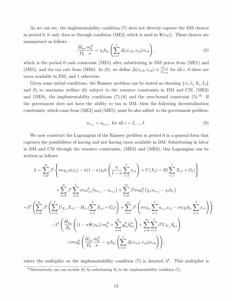
As we can see, the implementability condition (7) does not directly capture the DM choices

in period 0, it only does so through condition (ME2) which is used in Ψ(x0)). These choices are

summarized as followsHL0

P0

mN0

κ= χlhl0

(I∑i=1

∆(x1,0, xi,0)xi,0

), (8)

which is the period 0 cash constraint (ME4) after substituting in DM prices from (ME1) and

(ME5), and the tax rate from (ME6). In (8), we define ∆(x1,0, xi,0) ≡ uxi,0ux1,0

for all i, if there are

taxes available in DM, and 1 otherwise.

Given some initial conditions, the Ramsey problem can be stated as choosing xt, lt, Xt, Ltand P0 to maximize welfare (6) subject to the resource constraints in DM and CM, (ME3)

and (ME8), the implementability conditions (7)-(8) and the zero-bound constraint (5).16 If

the government does not have the ability to tax in DM, then the following decentralization

constraints, which come from (ME2) and (ME5), must be also added to the government problem:

uxi,t = ux1,t , for all i = 2, ..., I. (9)

We now construct the Lagrangian of the Ramsey problem in period 0 in a general form that

captures the possibilities of having and not having taxes available in DM. Substituting in labor

in DM and CM through the resource constraints, (ME3) and (ME8), this Lagrangian can be

written as follows

L =∞∑t=0

βt

σκχxu(xt)− σ(1− κ)χlh

(κ

1− κ

I∑i=1

xi,t

)+ U(Xt)−H(

I∑i=1

Xi,t +Gt)

+∞∑t=0

βtI∑i=2

σκϕ0i,t

(uxi,t − ux1,t

)+∞∑t=0

βtσκµ0t

(χxux1,t − χlhlt

)+λ0

(∞∑t=0

βt

(I∑i=1

UXi,tXi,t −HLt(I∑i=1

Xi,t +Gt)

)+∞∑t=1

βt

(σκχx

I∑i=1

uxi,txi,t − σκχlhltI∑i=1

xi,t

))

−λ0

(HL0

P0

((1− σΨ(x0))mN

0 +∞∑s=0

qN0,sbN0,s

)+∞∑s=0

I∑i=1

βtUXi,sbi0,s

)

+σκη00

(HL0

P0

mN0

κ− χlhl0

(I∑i=1

∆(x1,0, xi,0)xi,0

));

where the multiplier on the implementability condition (7) is denoted λ0. This multiplier is

16Alternatively, one can include (8) by substituting P0 in the implementability condition (7).

13

strictly positive and measures the cost of distortionary taxation. The multiplier corresponding

to condition (8) is denoted η00, which is strictly positive and measures the gains from ensuring a

monetary equilibrium in DM in period 0. The multipliers on the decentralization (9) and zero

bound constraints (5) are given by ϕ0i,t and µ0

t , respectively.17 In all previous multipliers, the

superscript 0 denotes that the choices are made by the government in period 0. As previously

mentioned, this Lagrangian allows for the possibilities of having (or not) taxes in DM. When

taxes are available in DM, we set ϕ0i,t = 0 and ∆(x1,0, xi,0) =

uxi,0ux1,0

. When they are not available,

we set Ψ(x0) = 0 and ∆(x1,0, xi,0) = 1.

Recall that qN0,0 = 1 and qN0,s =∏s

k=11

(1+rNk )=∏s

k=11(

σ χxχl

ux1,khlk

+(1−σ)

) for s ≥ 1. Then qN0,s is

a function of solely (x1,t, ..., xI,t)st=1. To keep track of its partial derivatives, we define

θi,t0,s ≡1

βtσκχxuxi,txi,t

HL0

P0

∂qN0,s∂xi,t

for all s ≥ 1, and for all i = 1, ..., I.

Then, the first order conditions for Xi,t for all i ≥ 1 and t ≥ 0 are given by18

∂

∂Xi,t

:(1 + λ0

)UXi,t + λ0UXi,tXi,t

(Xi,t − bi0,t

)= (1 + λ0)HLt + λ0HLt,LtLt. (10)

Similarly, the first order conditions for xi,t for all i ≥ 1 and t ≥ 1 are given by

∂

∂xi,t:(1 + λ0

)χxuxi,t+λ

0χxuxi,txi,t

(xi,t −

∞∑s=t

θi,t0,sbN0,s

)+Σ0

i,t = (1+λ0)χlhlt+λ0χlhlt,ltlt, (11)

which in period 0 become

∂

∂xi,0: χxuxi,0 + Σ0

i,t + λ0HL0

P0

mN0

1

κΨxi,0

=

(1 + η0

0

(∆(x1,0, xi,0) +

I∑j=1

∆xi,0xj,0

))χlhl0 + η0

0χlhl0,l0κ

1− κ

(I∑i=1

∆(x1,0, xi,0)xi,0

), (12)

with

Σ0i,t =

−∑N

i=2 ϕ0i,tux1,t,x1,t + µ0

t

(χxux1,tx1,t − χl κ

1−κhlt,lt)

for i = 1

ϕ0i,tuxi,t,xi,t − µ0

tχlκ

1−κhlt,lt for all i ≥ 2

.

17The multipliers on (5), (8) and (9) are multiplied by σκ to economize on notation.18The first order condition in period 0 already includes equation (13).

14

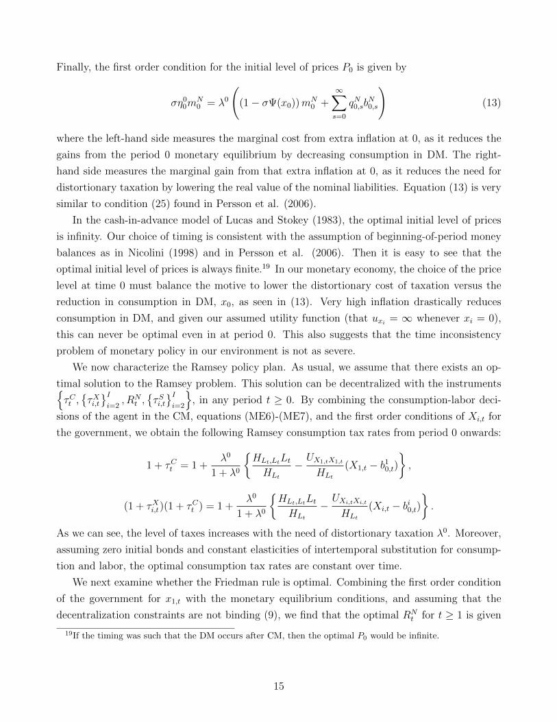
Finally, the first order condition for the initial level of prices P0 is given by

ση00m

N0 = λ0

((1− σΨ(x0))mN

0 +∞∑s=0

qN0,sbN0,s

)(13)

where the left-hand side measures the marginal cost from extra inflation at 0, as it reduces the

gains from the period 0 monetary equilibrium by decreasing consumption in DM. The right-

hand side measures the marginal gain from that extra inflation at 0, as it reduces the need for

distortionary taxation by lowering the real value of the nominal liabilities. Equation (13) is very

similar to condition (25) found in Persson et al. (2006).

In the cash-in-advance model of Lucas and Stokey (1983), the optimal initial level of prices

is infinity. Our choice of timing is consistent with the assumption of beginning-of-period money

balances as in Nicolini (1998) and in Persson et al. (2006). Then it is easy to see that the

optimal initial level of prices is always finite.19 In our monetary economy, the choice of the price

level at time 0 must balance the motive to lower the distortionary cost of taxation versus the

reduction in consumption in DM, x0, as seen in (13). Very high inflation drastically reduces

consumption in DM, and given our assumed utility function (that uxi = ∞ whenever xi = 0),

this can never be optimal even in at period 0. This also suggests that the time inconsistency

problem of monetary policy in our environment is not as severe.

We now characterize the Ramsey policy plan. As usual, we assume that there exists an op-

timal solution to the Ramsey problem. This solution can be decentralized with the instrumentsτCt ,τXi,tIi=2

, RNt ,τSi,tIi=2

, in any period t ≥ 0. By combining the consumption-labor deci-

sions of the agent in the CM, equations (ME6)-(ME7), and the first order conditions of Xi,t for

the government, we obtain the following Ramsey consumption tax rates from period 0 onwards:

1 + τCt = 1 +λ0

1 + λ0

HLt,LtLtHLt

−UX1,tX1,t

HLt

(X1,t − b10,t)

,

(1 + τXi,t)(1 + τCt ) = 1 +λ0

1 + λ0

HLt,LtLtHLt

−UXi,tXi,tHLt

(Xi,t − bi0,t).

As we can see, the level of taxes increases with the need of distortionary taxation λ0. Moreover,

assuming zero initial bonds and constant elasticities of intertemporal substitution for consump-

tion and labor, the optimal consumption tax rates are constant over time.

We next examine whether the Friedman rule is optimal. Combining the first order condition

of the government for x1,t with the monetary equilibrium conditions, and assuming that the

decentralization constraints are not binding (9), we find that the optimal RNt for t ≥ 1 is given

19If the timing was such that the DM occurs after CM, then the optimal P0 would be infinite.

15

by20

RNt = 1 + σ

λ0

1 + λ0

hlt,ltlthlt

− χxχl

ux1,t,x1,thlt

(x1,t −

∞∑s=t

θ01,tb

N0,s

), (14)

which, for zero initial nominal bonds maturing after period 1, implies a nominal interest rate,

RNt −1, that is strictly positive and increasing with the need of distortionary taxation λ0. There-

fore, the Friedman rule is not optimal in our search-theoretical economy, even at steady state.

This result is consistent with Aruoba and Chugh (2010) who consider an environment where the

government can commit to future policies. As opposed to these authors, our interpretation for

the Friedman rule not being optimal relates to the number of tax instruments available, as also

discussed in Kocherlakota (2005). A general consumption tax in DM, similar to τCt in CM, could

replace the inflation tax and nominal interest rates could be set to zero.

As for period 0, consider that taxes are available and optimally uniform in DM, then the first

order condition for xi,0 can be written as

χxuxi,0 =(1 + η0

0

)χlhl0 + η0

0χlhl0,l0l0, (15)

which, after substituting η00 from (13) we get

RN0 = 1 + λ0

(mN

0 +∑∞

s=0 qN0,sb

N0,s

mN0

)(1 +

hl0,l0hl0

l0

).

Therefore the optimal nominal interest rate in period 0 is also strictly positive and increases

with the cost of distortionary taxation λ0 as well as the amount of initial nominal bonds relative

to money holdings. Note also that from (15), η00 can be written as an increasing function of the

initial optimal nominal interest rate.

If sales taxes are available in DM, the optimal sales tax rate on good i for period t ≥ 1 can

be similarly obtained from

RNt

1− τSi,t= σ + σ

λ0

1 + λ0

hlt,ltlthlt

− χxχl

uxi,t,xi,thlt

(xi,t −

∞∑s=t

θ0i,tb

N0,s

)+ (1− σ)

uxi,tux1,t

.

If the utility function u(·) is homothetic, then uniform commodity taxation in DM is optimal.

Then all DM goods would be subject to the inflation tax implied by (14) and sales tax rates

would be set to zero, τSi,t = 0 for all i ≥ 2.

In the next Section, we study whether the Ramsey policy plan, that we just characterized,

is time consistent.

20When taxes in DM are not available and the decentralization constraints (9) bind, the optimal level of nominalinterest rates will be affected by the additional relative motives for taxation, just as in Correia (1996)’s model ofincomplete taxation.

16

4 Time Consistency of the Optimal Policy

As usual, the structure of government bonds is irrelevant in the economy with commitment. In

other words, the real value of total government liabilities is uniquely determined by the Ramsey

allocation, but the composition and maturity of these obligations are not. In this Section, we

explore whether there is an optimal structure of real and nominal government bonds that makes

the optimal fiscal and monetary policy time consistent.

In our search-theoretic economy, we find the following result.

Proposition 1 Optimal fiscal and monetary policies are in general time inconsistent.

Proof: See Appendix.

Proposition 1 emphasizes the fact that in this environment we have a limited debt struc-

ture and therefore not enough instruments to guarantee time consistency. Following Tinbergen

(1956)’s reasoning, a government requires at least as many debt instruments as policies to in-

duce the next government to not deviate and to optimally continue with the Ramsey policy plan

previously selected. Taking further Tinbergen’s arguments, we find that time consistency can

be imposed in some circumstances as stated in the next proposition.

Proposition 2 There exists an optimal structure of real and nominal government bonds that

makes the optimal fiscal and monetary policies time consistent whenever

(i) taxes in DM are not available;

(ii) taxes in DM are available and satisfy the conditions for optimal uniform taxation.

Proof: See Appendix.

As we can see from Proposition 1 and 2, there are two important cases where time consistency

can be restored. First, if taxes in the decentralized anonymous markets are not available, the

multipliers on the decentralization constraints, which are not determined by the allocation,

can be utilized as additional instruments to ensure time consistency.21 Second, if taxes in the

decentralized markets are available, time consistency arises when the different decentralized

market goods satisfy the conditions necessary for optimal uniform commodity taxation. However,

if the government finds optimal to use non-uniform taxation across goods in decentralized markets

and has access to such taxation in these markets, then optimal fiscal and monetary policies are

time inconsistent.

21A similar result is found in a capital taxation problem by Domınguez (2007). The author finds that inproblems where a unique debt structure guarantees time consistency, multiplicity of optimal debt structuresarise if there are additional constraints on the implementable allocation that introduce extra multipliers in thegovernment problem. For example, imposing that capital tax rates cannot be above 100 %, if binding, generatesmultiplicity.

17

When time consistency is restored, the optimal debt structure is very similar to the one

found by Persson et al. (2006). Eliminating the incentives to increase the initial level of prices

implies an overall amount of nominal bonds issues relative to money holdings for which initial

net nominal liabilities are positive. Eliminating the incentives to deviate from the previously

chosen DM taxes determines the maturity of the nominal bonds.

In our economy the Friedman rule is not optimal. We next examine situations where the

Friedman rule can be optimal and re-examine the results of Alvarez et al. (2004). Consider

instantaneous utility functions u(·) and h(·) that solve the Ramsey problem and that satisfy the

optimal Friedman rule χxux1,t = χlhl,t. Here we are thinking of allowing for a positive satiation

level for good 1, x1, so that u(·) would not satisfy monotonicity neither concavity for good 1 while

maintaining all previous assumptions regarding all other decentralized markets goods. Then, it

is easy to see, that our monetary economy is still not identical to a real economy. Even if nominal

interest rates are optimally zero, the government still faces a taxation problem in decentralized

markets. And, if taxes in decentralized markets are available and optimally different across

goods, then optimal fiscal and monetary policies are time inconsistent. This time inconsistency

is a direct consequence of the inability to influence the fiscal choices in decentralized markets.

Then the results of Alvarez et al. (2004), that ensure that optimal policies are time consistent

when the Friedman is satisfied, are not applicable in this environment.

5 Conclusions

This paper has investigated the time consistency of optimal monetary and fiscal policies in

economies with multiple consumer goods. We have shown that when there are many government

policy decisions per period affecting nominal variables, optimal monetary and fiscal policies are

in general time inconsistent. The main reason behind this result is that there are insufficient

instruments to influence future governments’ decisions. The insufficiency of debt instruments is

a necessary condition for the existence of money. If governments could issue bonds that pay the

right cash goods at the right time/location, fiat money would not be essential.

Furthermore, we find that the frictions that make money essential in our economy are also

relevant for time consistency. If the anonymity and lack of enforcement in decentralized markets

are such that preclude governments from taxing agents in these markets, then optimal monetary

and fiscal policies are time consistent. If, on the other hand, the government can enforce taxation

on anonymous individuals (by, for example, taxing the firms where they work in these decentral-

ized markets), then optimal policies will be time inconsistent when the different decentralized

markets goods require an optimal non-uniform tax. These results are a direct consequence of

how fiat money is modeled which has important implications for other parts of the model as em-

phasized by Wallace (2001). The framework in this paper highlights how informational frictions

18

that make fiat money essential affect the debt and tax instruments available which in turn affect

the time consistency of optimal fiscal and monetary policies.

We believe that our results are an example of a broader issue. The nominal submarket with

multiple goods and informational frictions imposes restrictions on the feasible debt instruments,

and nominal bonds can only influence one aspect of the nominal basket but not all its compo-

nents in a different way. In this paper, we have adopted a large family approach, where all the

randomness of the location assignment are smoothed out, and have ignored the possibility of a

random matching process leading to different ex-post realizations. If we had included these addi-

tional frictions in the environment, the additional information from one period to the next would

provide an additional motive for future governments to deviate from previous announcements.

References

[1] Aiyagari, R., N. Wallace and R. Wright (1996). “Coexistence of Money and Interest-bearing

Securities,” Journal of Monetary Economics, 37, 397-419.

[2] Aruoba, B. and S. Chugh (2010). “Optimal Fiscal and Monetary Policy when Money is

Essential,” Journal of Economic Theory, 145, 1618-1647.

[3] Aruoba, B., G. Rocheteau, and C. Waller (2007). “Bargaining and the Value of Money,”

Journal of Monetary Economics, 54, 2636-2655.

[4] Alvarez, F. and M. Veracierto (2000). “Labor-Market Policies in an Equilibrium Search

Model,” NBER Macroeconomics Annual 1999, vol. 14, 265-316.

[5] Alvarez, F., P. Kehoe and P. Neumeyer (2004). “The Time Consistency of Optimal Monetary

and Fiscal Policies,” Econometrica, 72, 541-567.

[6] Calvo, G. A. (1978). “On the Time Consistency of Optimal Policy in a Monetary Economy,”

Econometrica, 46, 1411-28.

[7] Correia, I. H. (1996). “Should Capital Income be Taxed in the Steady State?,” Journal of

Public Economics, 60, 147-151.

[8] Domınguez, B. (2007). “On the Time-Consistency of Optimal Capital Taxes,” Journal of

Monetary Economics, 54, 686-705.

[9] Gomis-Porqueras, P. and A. Peralta-Alva, (2010). “Optimal Monetary and Fiscal policies

in a Search Theoretic Model of Monetary Exchange,” European Economic Review, 54(3),

331-344.

19

[10] Kocherlakota, N. (1998). “Money is Memory,” Journal of Economic Theory, 81, 232-251.

[11] Kocherlakota, N. (2005). “Optimal Monetary Policy: What We Know and What We don’t

Know,” International Economic Review, 46, 305-16.

[12] Lagos, R., and R. Wright (2005). “A Unified Framework for Monetary Theory and Policy

Analysis,” Journal of Political Economy, 113, 463-484.

[13] Li, Y., G. Rocheteau, and P. Weill (2011) “Liquidity and the Threat of Fraudulent Assets,”

NBER Working Papers 17500, National Bureau of Economic Research, Inc October.

[14] Lucas, R. and E. Prescott (1974). “Equilibrium Search and Unemployment,” Journal of

Economic Theory, 7(2), 188-209.

[15] Lucas, R. and N. Stokey (1983). “Optimal Fiscal and Monetary Policy in an Economy

without Capital,” Journal of Monetary Economics, 12, 55-93.

[16] Martın , F. (2011). “On the Joint Determination of Fiscal and Monetary Policy,” Journal

of Monetary Economics, 58, 132-145.

[17] Martın , F. (2012a). “Government Policy in Monetary Economies,” International Economic

Review, Forthcoming.

[18] Martın , F. (2012b). “Government Policy Response to War-Expenditure Shocks,” The B.E.

Journal of Macroeconomics, Forthcoming.

[19] Nicolini, J. P. (1998). “More on the Time Consistency of Monetary Policy,” Journal of

Monetary Economics, 41, 333-350.

[20] Persson, M., T. Persson and L. Svensson (2006). “Time Consistency of Fiscal and Monetary

Policy: A Solution,” Econometrica, 74, 193-212.

[21] Shi, S. (1997). “A Divisible Search Model of Fiat Money,” Econometrica, 65, 75-102.

[22] Tinbergen, J. (1956). Economic Policy: Principles and Design, Amsterdam, North-Holland.

[23] Wallace, N. (1983). “A Legal Restrictions Theory of the Demand for ’Money’ and the Role

of Monetary Policy,” Federal Reserve Bank of Minneapolis Quarterly Review, 1-7.

[24] Wallace, N. (2001). “Whither Monetary Economics?,” International Economic Review, 42,

847-69.

20

Appendix

The Implementability Condition

The buyer’s consumption is determined by the cash constraint (ME4) which, multiplied by

βtχxux1,tp1,t

and using (ME5), becomes

σκI∑i=1

βtχxuxi,txi,t = βtσχxux1,tp1,t

mNt . (16)

The seller’s decision is given by the first order condition (ME1), which multiplied by −βtp1,tlt,

and using (ME2)-(ME4), can be written as

−βtσ(1− κ)χlhltlt = −βt(σmN

t − TDMt

) UX1,t

Pt(1 + τCt ). (17)

We next write TDMt = σκ∑I

i=2 pi,tτSi,txi,t in terms of allocation. From (ME2) and (ME5), we

obtain pi,t = p1,tuxi,tux1,t

and τSi,t = 1− ux1,tuxi,t

. From (16), we get p1,t =ux1,t∑I

i=1 uxi,txi,t

mNtκ. Therefore, we

find

TDMt = σΨ(xt)mNt , where Ψ(xt) ≡

∑Ii=2

(uxi,t − ux1,t

)xi,t∑I

i=1 uxi,txi,t.

Adding equations (16)-(17), we summarize DM in

βt

(σκχx

I∑i=1

uxi,txi,t − σ(1− κ)χlhltlt

)= βt

(σ

(χxχl

ux1,thlt− 1

)+ σΨ(xt)

)mNt

UX1,t

Pt(1 + τCt ).

(18)

This equation, (18), in period 0 simplifies to (8).

After DM, given our structure, the household’s money holdings are mNt − TDMt . Multiplying

the budget constraint (2) by βtUX1,t

Pt(1+τCt ), and using conditions (ME6) and (ME7), we get

βt

(I∑i=1

UXi,tXi,t −HLtLt

)=

βtUX1,t

Pt(1 + τCt )

(mNt − σΨ(xt)m

Nt −mN

t+1 +∞∑s=t

qNt,sbNt,s −

∞∑s=t+1

qNt,sbNt+1,s +

∞∑s=t

I∑i=1

qit,sbit,s −

∞∑s=t+1

I∑i=1

qit,sbit+1,s

).

(19)

As CM opens in period 0 after DM, we add equation (19) from t ≥ 0 and condition (18) from

21

period 1 onwards, to obtain

∞∑t=0

βt

(I∑i=1

UXi,tXi,t −HLtLt

)+∞∑t=1

βt

(σκχx

I∑i=1

uxi,txi,t − σ(1− κ)χlhltlt

)=

(1− σΨ(x0))mN0

UX1,0

P0(1 + τC0 )+∞∑t=1

βt−1

(β

(σχxχl

ux1,thlt

+ 1− σ)

UX1,t

Pt(1 + τCt )−

UX1,t−1

Pt−1(1 + τCt−1)

)mNt +

∞∑t=0

βtUX1,t

Pt(1 + τCt )

(∞∑s=t

qNt,sbNt,s −

∞∑s=t+1

qNt,sbNt+1,s +

∞∑s=t

I∑i=1

qit,sbit,s −

∞∑s=t+1

I∑i=1

qit,sbit+1,s

). (20)

Imposing the necessary conditions (ME6)-(ME8), the RHS of (20) becomes

HL0

P0

((1− σΨ(x0))mN

0 +∞∑s=0

qN0,sbN0,s + P0

∞∑s=0

I∑i=1

qi0,sbi0,s

).

Finally, using qi0,s = βsUXi,s1

UXi,0, the implementability condition becomes

∞∑t=0

βt

(I∑i=1

UXi,tXi,t −HLtLt

)+∞∑t=1

βt

(σκχx

I∑i=1

uxi,txi,t − σ(1− κ)χlhltlt

)=

HL,0

P0

((1− σΨ(x0))mN

0 +∞∑s=0

qN0,sbN0,s

)+∞∑s=0

I∑i=1

βsUXi,sbi0,s.

Proof of Propositions 1 and 2.

Let us first present the Ramsey allocations chosen by the government at 0 and the government

at 1. The Ramsey allocation evaluated at date 0 for all t ≥ 1 is summarized in:

(1 + λ0

)UXi,t + λ0UXi,tXi,t

(Xi,t − bi0,t

)= (1 + λ0)HLt + λ0HLt,LtLt, (21)

(1 + λ0

)χxuxi,t + λ0χxuxi,txi,t

(xi,t −

∞∑s=t

θi,t0,sbN0,s

)+ Σ0

i,t = (1 + λ0)χlhlt + λ0χlhlt,ltlt, (22)

together with the resource constraints, (ME3) and (ME8), the implementability constraint (7)

and, if taxes in DM are not available, the decentralization constraints (9).

The Ramsey allocation evaluated at date 1 is summarized in:

(1 + λ1

)UXi,t + λ1UXi,tXi,t

(Xi,t − bi1,t

)= (1 + λ1)HLt + λ1HLt,LtLt, ∀t ≥ 1 (23)

22

(1 + λ1

)χxuxi,t + λ1χxuxi,txi,t

(xi,t −

∞∑s=t

θi,t1,sbN1,s

)+ Σ1

i,t = (1 + λ1)χlhlt + λ1χlhlt,ltlt, ∀t ≥ 2

(24)

which in period 1 becomes

χxuxi,1 + Σ1i,t + λ1HL1

P1

mN1

1

κΨxi,1

=

(1 + η1

1

(∆(x1,1, xi,1) +

I∑j=1

∆xi,1xj,1

))χlhl1 + η1

1χlhl1,l1κ

1− κ

(I∑i=1

∆(x1,1, xi,1)xi,1

), (25)

where η11 satisfies

ση11m

N1 = λ1

((1− σΨ(x1))mN

1 +∞∑s=0

qN1,sbN1,s

), (26)

together with the resource constraints, (ME3) and (ME8), the implementability constraints (7)

and (8) evaluated in period 1, and, if necessary, the decentralization constraints (9).

We now explore whether the government at date 0 can design a debt structure that eliminates

the incentives to deviate, by the government at date 1, from the Ramsey plan chosen at date 0. To

do this, we first assume that the Ramsey allocation evaluated in period 0 solves also the Ramsey

problem in period 1 and then we check whether the existing debt instruments are sufficient to

guarantee that. Note that the resource constraints, (ME3) and (ME8), and decentralization

constraints (9) are the same in both plans and therefore do not pose any additional incentives

to deviate. The initial level of prices is a function of the first period allocation, equation (8)

evaluated in period 1, and will be satisfied as long as we guarantee the same allocation.

First, we analyze the CM choices, Xi,t for all t ≥ 1, by subtracting (21) from (23) and solving

for the real bonds inherited by the government at date 1:

bi1,t =

(λ0

λ1

)bi0,t +

(1− λ0

λ1

)(Xi,t +

UXi,tUXi,tXi,t

− HLt +HLt,LtLtUXi,tXi,t

). (27)

Next, we study the first period DM choices, xi,1, by subtracting (22) at t = 1 from (25),

substituting the value of η11 from the condition for P1 by the government at 1, (26), which yields(

(1− σΨ(x1))mN1 +

∑∞s=0 q

N1,sb

N1,s

mN1

)− σHL1

P1

mN1

κ

Ψxi,1

Ω(x1)−(

Σ1i,1 − Σ0

i,1

λ1

)σ

Ω(x1)

=λ0

λ1

σ

Ω(x1)

(χl (hl1 + hl1,l1l1)− χx

(uxi,1 + uxi,1xi,1

(xi,1 −

∞∑s=1

θi,10,sbN0,s

))), (28)

where we denote Ω(x1) = χlhl1

∆(x1,1, xi,1) +

∑Ij=1 ∆xi,1xj,1 +

(κ

1−κ∑Ii=1 ∆(x1,1,xi,1)xi,1

l1

)hl1,l1 l1hl1

.

23

Then, we focus on the DM choices, xi,t for all t ≥ 2, by subtracting (22) from (24) and solving

for the nominal bonds inherited by the government at date 1, which are as follows:

∞∑s=t

θi,t1,sbN1,s −

(Σ1i,1 − Σ0

i,1

λ1

)1

χxuxi,txi,t=

(λ0

λ1

) ∞∑s=t

θi,t0,sbN0,s +

(1− λ0

λ1

)(xi,t +

uxi,tuxi,txi,t

− χlχx

(hlt + hlt,ltltuxi,txi,t

)). (29)

In the above, we have presumed that the same Ramsey allocation from period 1 onwards

solves the policy plans evaluated at date 0 and at date 1. If there were a solution to the above

system of bonds (27)-(29), these equations can be imposed onto the implementability condition

(7) for the government in period 1 and would provide the value of λ1. Plugging back this value

of λ1, the equations (27)-(29) would be the optimal real and nominal bond structure that would

induce the government in period 1 to follow the Ramsey policy plan evaluated by the government

at date 0. By induction, the same it is true for all later periods, and optimal fiscal and monetary

policies would be time consistent.

Now the question is under which conditions there exists a solution to the above system of

bonds (27)-(29) for all i = 1, ..., I and all t ≥ 1. First, for real bonds (27), we have as many

real bonds I as CM consumption-labor decisions I in each period. Therefore, the real economy

counts with the exact number of instruments required for time consistency. Second, for nominal

bonds, (28) and (29), we have only one nominal bond bNt per period for all DM consumption-

labor decisions. If the number of DM consumer goods would be one, the nominal economy would

count with the required number of instruments. However, if the number of DM consumer goods

is I > 1, we have in principle less instruments than those necessary.

If tax rates in DM are not available, then the decentralization constraints (9) imply

Σ1i,t =

−∑N

i=2 ϕ1i,tux1,t,x1,t for i = 1

ϕ1i,tuxi,t,xi,t for all i ≥ 2

.

The multipliers ϕ1i,t are not determined by the Ramsey allocation. For a given period t ≥ 2,

one can pick the new issues of nominal bonds that solves (29) for good 1 and the multiplier ϕ1i,t

that solves (29) for all other i ≥ 2. Similarly for period 1, but solving (28). Plugging them back

together with the real bonds (27) into the implementability condition for the government at 1,

this implies a multiplier λ1 that exactly delivers those decentralization multipliers ϕ1i,t and the

same allocation and policy as the ones chosen by the government at period 0.

If tax rates in DM are available, then Σ1i,1 = Σ0

i,1 = 0. Note also that the value of uxi,t,xi,tθi,t1,s

is determined solely by the nominal interest rate RNt+1 − 1 = σ

(χxχl

ux1,t+1

hlt+1− 1)

and the Ramsey

24

allocation, just as UXi,t,Xi,t for real bonds (27). Then, in general, there is no one bNt that satisfies

(28) and (29) for all DM goods i = 1, ..., I. If there were one DM good, equation (28) would

determine the total amount of new nominal bonds (relative to money holdings). This amount is

not good specific and cannot adjust to the different requirements of each DM good i as the right-

hand side of the equation requires. If there were one DM good, equation (29) would determine

the new issues of nominal bonds for each maturity s ≥ 1. This amount is again not good specific

as the right-hand side of the equation requires. Therefore, optimal monetary and fiscal policies

are, in general, time inconsistent.

However, when sales tax rates in DM satisfy the conditions required for optimal uniform

commodity taxation, i.e. u(·) is homothetic, then uxi,t = ux1,t for all i ≥ 2 in each period and

nominal interest rates RNt+1 − 1, can now be written as a function of the consumption of each

DM good:

RNt+1 − 1 = σ

(χxχl

ux1,t+1

hlt+1

− 1

)= σ

(χxχl

(φ1

1,t+1ux1,t+1 + ...+ φ1I,t+1uxI,t+1

)hlt+1

− 1

),

where∑I

i=1 φ1i,t+1 = 1. Note that without optimal uniform commodity taxation, RN

t+1 can only

be written as a function of the allocation when it is written in terms of the consumption of DM

good 1; otherwise sales tax rates would appear in the above equation. Then the government

in period 0 can now choose each φ1i,t that implies a θi,t1,s, which solves (28) and (29) for all

i ≥ 2 and let the total amount of new issues of nominal bonds solve (28) for i = 1 and the

new issues at each maturity solve (29) also for i = 1.22 By doing this, together with the real

bonds (27), the government at 0 can provide the right incentives for the government at 1 to

continue with the Ramsey plan evaluated at 0. Then, optimal monetary and fiscal policies

are time consistent. Alternatively, this can be understood by looking at the Ramsey nominal

interest rate and noticing that optimal uniform taxation requires zero sales taxes for all i ≥ 2

and therefore only one decision per period (not per DM good) needs to be influenced by the

government in period 0.

22Taking into account this possibility, when taxes are not available in DM, there would be multiple debtstructures that solve the time inconsistency problem.

25