on the tidal dynamics of the north sea - utwente.nl · external supervisor: drs. a. stolk...
TRANSCRIPT


ON THE TIDAL DYNAMICS OF THE NORTH SEA
An idealised modelling study on the role of bottom friction, the Dover Strait and tidal
resonance in the North Sea.
Enschede, 17 September 2010.
ThiThiThiThis master thesis was written bys master thesis was written bys master thesis was written bys master thesis was written by
Jorick J. Velema BSc.
aaaas fulfilment of the Master’s degree s fulfilment of the Master’s degree s fulfilment of the Master’s degree s fulfilment of the Master’s degree
Water Engineering & Management, University of Twente, The Netherlands
uuuunder the supervision of the following committeender the supervision of the following committeender the supervision of the following committeender the supervision of the following committee
Daily supervisor: Dr. ir. P.C. Roos (University of Twente)
Graduation supervisor: Prof. dr. S.J.M.H. Hulscher (University of Twente)
External supervisor: Drs. A. Stolk (Rijkswaterstaat Noordzee)


i
This thesis is a study on the tidal dynamics of the North Sea, and in particular on the role of
bottom friction, the Dover Strait and tidal resonance in the North Sea. The North Sea is one of the
world’s largest shelf seas, located on the European continent. There is an extensive interest in its
tide, as coastal safety, navigation and ecology are all affected by it. The tide in the North Sea is a
co-oscillating response to the tides generated in the North Atlantic Ocean. Tidal waves enter the
North Sea through the northern boundary with the North Atlantic Ocean and through the Dover
Strait. Elements which play a possible important role on the tidal dynamics are bottom friction,
basin geometry, the Dover Strait and tidal resonance.
The objective of this study is to understand the large-scale amphidromic system of the North Sea,
and in particular (1) the role of bottom friction, basin geometry and the Dover Strait on North Sea
tide and (2) the resonant properties of the Southern Bight. In addition, a case study was
performed, to analyze the effects of a giant scale windmill park in the Southern Bight, represented
by an increase in bottom friction. To this end a process-based idealized Taylor model was setup,
which allows box schematised geometries, a linear bottom friction coefficient and two forced tidal
waves. The model is an extension to Taylor’s (1921) model and solves the tide as a superposition of
Kelvin and Poincaré waves.
The geometry of the North Sea is schematised as series of adjacent rectangular sub-basins, which
may vary in length, width and uniform depth. The model is forced by two incoming Kelvin waves,
i.e. entering through the Northern boundary with the Atlantic Ocean and through the Dover
Strait. The forced waves, together with a relative friction coefficient, were calibrated on tidal data
along the perimeter of the model basin, for the M2-, S2-, K1- and O1-tidal constituents.
The model was well capable of simulating the tidal ranges of the M2-, S2-, K1- and O1-tidal
constituents in the North Sea. The simulated tidal phase showed good results along the west coast
of the North Sea and along the perimeter of the Southern Bight. A structural error in the
simulated tidal phase was seen along the east coast of the North Sea. This was probably caused by
the Skagerrak, which was not involved in the representative model basin of the North Sea. Two
case simulations were performed regarding the bottom friction and the Dover Strait. It was found
that the Dover Strait acts as a source of tidal energy and fulfils a major role in the tidal dynamics
of the North Sea. Further it was found that the bottom friction mainly causes damping of the tidal
ranges.
The state of tidal resonance in the Southern Bight was analyzed including rotation. It was found
that the M2-, S2-, K1- and O1-tidal constituents are currently not in a state of resonance and are
also not sensitive to tidal resonance, with respect to changes in geometry. Further it was found
that the direct effects of a giant scale windmill park in the Southern Bight on the tidal ranges in
the North Sea are of a minor scale.
Abstract

ii

iii
This thesis was written as culmination of the Master study Water Engineering and Management,
University of Twente, the Netherlands. It contains the results of ten months of work, including
pre-studies. The process of setting up a research and finishing it, was a process from which I
learned a lot. The model which I wrote for this study became a thing itself, which I continuously
tried to improve. In total I wrote about 3000 unique lines of model script, which corresponds to
the lines written in this thesis.
Within the last lines I write, I’d like to thank some people. First of all my graduation committee:
Suzanne Hulscher, Pieter Roos and Ad Stolk. Especially Pieter, for his willing to teach me a lot
about the world of mathematics and helping me out when I was stuck. Second I like to thank my
lovely girl Lena, for her enormous help correcting my spelling and her sweet kisses while I tried to
think of something ingenious. I would also like to thank my buddies at the Afstudeerkamer for the
good times. Last but not least, I would like to thank Sierd. Not for the good advice, but for the well
needed nonsense and a good friendship.
With this thesis I’ll end my time as a student at the University of Twente. I hope you enjoy
reading my last piece, as a student!
Jorick Velema
Enschede, September 2010
Preface

iv
Abstract ....................................................................................................................................... i
Preface....................................................................................................................................... iii
Table of contents ....................................................................................................................... iv
List of frequently used symbols ................................................................................................ vi
1. Introduction ........................................................................................................................- 1 -
1.1. The North Sea (tide) ....................................................................................................- 1 -
1.2. Idealized process-based Taylor models.......................................................................- 2 -
1.3. Tidal resonance ...........................................................................................................- 3 -
1.4. Purpose of this study ...................................................................................................- 4 -
2. Research approach..............................................................................................................- 5 -
2.1. Geometric and tidal data .............................................................................................- 5 -
2.2. The tidal dynamics of the North Sea...........................................................................- 6 -
2.3. Tidal resonance Southern Bight ..................................................................................- 8 -
2.4. Windmill park Southern Bight ....................................................................................- 8 -
3. Theoretical background......................................................................................................- 9 -
3.1. Basin Geometries ........................................................................................................- 9 -
3.2. Nonlinear shallow water equations .............................................................................- 9 -
3.2.1. Boundary conditions ..........................................................................................- 10 -
3.3. Linear shallow water equations.................................................................................- 10 -
3.4. Wave solutions linear shallow water equations in an infinite channel ....................- 11 -
3.4.1. Eigenvalue relation.............................................................................................- 12 -
3.4.2. Kelvin waves ......................................................................................................- 12 -
3.4.3. Poincaré waves...................................................................................................- 13 -
3.5. Taylor problem..........................................................................................................- 14 -
4. Extended Taylor model: abrupt width- and depth-changes .............................................- 17 -
4.1. Model setup ...............................................................................................................- 17 -
4.1.1. Basin setup .........................................................................................................- 17 -
4.1.1.1. Boundary conditions ...................................................................................- 18 -
4.1.2. Linear shallow water equations..........................................................................- 19 -
4.2. Solution method ........................................................................................................- 19 -
4.2.1. Collocation points ..............................................................................................- 20 -
4.2.2. Linear system .....................................................................................................- 21 -
5. Tidal dynamics in the North Sea ......................................................................................- 22 -
5.1. Model basin setup......................................................................................................- 22 -
5.2. Calibration setup .......................................................................................................- 23 -
5.3. Simulation setup........................................................................................................- 23 -
5.4. Results basin setups (run 1-4) ...................................................................................- 24 -
5.5. Results tidal constituents (run 4-7)............................................................................- 25 -
5.6. Results no bottom friction (run 8-11) and no Dover Strait (run 12-15)....................- 27 -
Table of contents

v
6. Tidal resonance; physical mechanisms ............................................................................- 29 -
6.1. Basin setup ................................................................................................................- 29 -
6.2. Simulation setup........................................................................................................- 30 -
6.3. Results reference run.................................................................................................- 30 -
6.4. Results geometry, rotation and friction .....................................................................- 31 -
6.5. Results second open boundary ..................................................................................- 32 -
6.6. Summary results........................................................................................................- 33 -
7. Tidal resonance; Southern Bight ......................................................................................- 34 -
7.1. Setup tidal resonance in Southern Bight ...................................................................- 34 -
7.2. Results tidal resonance in Southern Bight.................................................................- 35 -
8. Windmill park; Southern Bight ........................................................................................- 36 -
8.1. Setup windmill park in the Southern Bight...............................................................- 36 -
8.2. Results windmill park in the Southern Bight ............................................................- 37 -
9. Discussion ........................................................................................................................- 38 -
9.1. Results ET-model......................................................................................................- 38 -
9.1.1. Model basin ........................................................................................................- 38 -
9.1.2. Reproduction of the tidal dynamics in the North Sea ........................................- 38 -
9.1.3. Tidal resonance in the Southern Bight ...............................................................- 39 -
9.1.4. Windmill park in the Southern Bight .................................................................- 39 -
9.2. Simplifications of the ET-model ..............................................................................- 39 -
10. Conclusions and recommendations................................................................................- 41 -
10.1. Recommendations and future research ...................................................................- 42 -
11. References ......................................................................................................................- 44 -
Appendix A - Scaling.................................................................................................................. I
Appendix B - Setup basins ....................................................................................................... III
Appendix C - Results North Sea ............................................................................................... V

vi
Symbol Unit Definition
A m Complex wave amplitude
0A m Complex wave amplitude forced wave sub-basin one (Northern)
dA0 m Complex wave amplitude forced wave sub-basin bN (Dover Strait)
b m Basin width
dC - Drag coefficient
wtdC _ - Drag coefficient windmill park
D m Lateral displacement between two sub-basin, see equation (20)
squaredE - Average scaled squared error
f s-1 Coriolis parameter
sf - Relative friction coefficient
aF - Scaled average tidal range over a specific sub-basin
cF - Scaled average tidal range at closest end model basin
g m s2 Earth’s gravitational acceleration
H m Mean water depth
k m-1 Wave number
l m Length sub-basin
L m Basin length
0L m Kelvin wave length
M - Number of collocation points
bn - Sub-basin number
bN - Total number of sub-basins
r m s-1 Linear friction coefficient
corrr - Correlation coefficient
fR m Frictional Rossby deformation radius
s s-1 Complex quantity, H
ri +− σ
S s-1 Complex quantity, H
r
t+
∂∂
t s Time
T s Wave period
u m s2 Depth-averaged velocity in longitudinal direction
u m s2 Complex amplitude of depth-averaged velocity in longitudinal direction
U m s2 Typical velocity scale Kelvin wave
v m s2 Depth-averaged velocity in lateral direction
v m s2 Complex amplitude of depth-averaged velocity in lateral direction
List of frequently used symbols
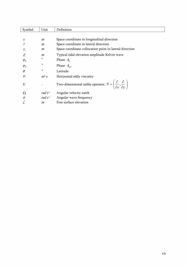
vii
Symbol Unit Definition
x m Space coordinate in longitudinal direction y m Space coordinate in lateral direction
cy m Space coordinate collocation point in lateral direction
Z m Typical tidal elevation amplitude Kelvin wave
0ϕ ° Phase 0A
dϕ ° Phase dA0
θ ° Latitude
µ m2 s Horizontal eddy viscosity
∇ - Two-dimensional nabla-operator,
∂∂
∂∂
=∇yx
,
Ω rad s-1 Angular velocity earth
σ rad s-1 Angular wave frequency
ζ m Free surface elevation


* A harmonic wave which represents an astronomic tidal component. - 1 -
With its surface area of 575.300km2, the North Sea is one of the world’s largest shelf seas
(Huthnance 1991). Bounded by the east coasts of Scotland and England to the west and the
northern and central European mainland to the east and south, the North Sea has seven
surrounding states (UK, France, Belgium, Netherlands, Germany, Denmark and Norway). The tide
of the North Sea is of an extensive interest to these states, as coastal safety, navigation and ecology
are all affected by the tide: directly through fluctuating water levels and oscillatory currents as
well as indirectly through the presence and dynamics of tide-induced bedforms (Huthnance
1991).
The North Sea is a shelf sea located on the European continent. It has a length of approximately
1000km and a width of approximately 550km (Carbajal 1997). With an averaged depth of 74m the
North Sea is relatively shallow (Otto et al. 1990). The bathymetry of the North Sea is shown in
figure 1. The southern part of the North Sea, the Southern Bight, is the most shallow part, with
averaged depths around a few tens of meters. Moving up north the depth increases. The deepest
point in the North Sea is found in a shore-parallel trench located near the Norwegian coast, with
depths over 500m.
The tidal motions in a shelf sea are not the result of the direct action of the tide-generating forces.
In fact, the observed tide in the North Sea is a co-oscillating response to the tidal waves generated
in the North Atlantic Ocean (Banner et al. 1979). The main tidal constituents* are expressed by
1. Introduction
1.1. The North Sea (tide)
Figure 1, Bathymetry of the North Sea, the red line
indicates the boundaries of the North Sea. Data
retrieved from US National Geophysical Data Center
(2010).
Figure 2, Amphidromic system of the M2-
tide in the North Sea (Dyke 2007). The
solid lines are the co-phase lines and the
dashed lines are the co-range lines.

* a wave pattern which rotates around an elevation amphidromic point**.
** point with no tidal range fluctuations in time.
*** rotating plane with a constant rotation rate.
- 2 -
waves which enter and exit the North Sea through an open boundary with the North Atlantic
Ocean in the north. However, through the Dover Strait in the south and the Skagerrak in the east
minor tidal constituents may also enter and exit the North Sea. The Dover Strait is the oversea
distance of approximately 35km between France and England. It connects the Southern Bight
with the English Channel, which again is connected to the North Atlantic Ocean. The Dover
Strait may either function as a source or a sink of tidal energy and may cause a phase shift on the
tidal constituents. The Skagerrak, located between Denmark and Norway, is of approximately
100km wide and connects the North Sea indirectly with the Baltic Sea. According to Otto et al.
(1990) the Skagerrak is mainly a sink of tidal energy.
In this study the North Sea tide is represented by the four largest tidal constituents in the North
Sea; i.e. (1) the semidiurnal lunar tide, M2-tide, (2) the semidiurnal solar tide, S2-tide, (3) the
diurnal luni-solar declinational tide, K1-tide and (4) the diurnal lunar declinational tide, O1-tide.
Table 1 shows the periods and a typical coastal amplitude of the M2-, S2-, K1- and O1-tidal
constituents and the amplitude ratios relative to the M2-tide. The ratios between the amplitudes of
the constituents are fairly stable over the North Sea, except near the amphidromic points (Pugh
1996).
Constituent Period Typical coastal amplitude Ratio M2-tide
hour m -
M2 12:25 1.61 1
S2 12:00 0.54 0.34
K1 23:57 0.14 0.08
O1 25:49 0.14 0.08 Table 1, the periods, a typical tidal amplitude and the amplitude ratios of the M2-, S2-, K1- and O1-tidal
constituents. Data retrieved from the British Admiralty (2010).
The most dominant tidal constituent in the North Sea is the M2-tide. Figure 2 shows the elevation
amphidromic system* of the M2-tide in the North Sea. Keeping the coast on its right, the M2 tidal
wave propagates in a counter clockwise direction through the main basin. Near the coast of
Scotland and England it propagates almost as a perfect Kelvin wave. This can be seen in the
rectangular pattern of the co-tidal and co-range lines in figure 2 (Dyke 2007). The spatial pattern
of the M2-tide is characterised by three elevation amphidromic points** (EAPs), one located in the
Southern Bight and two in the main basin.
Two approaches exist to model the tidal processes in the North Sea: numerical models with
realistic geometries to reproduce and predict tidal observations and idealized process-based models
to obtain insight into the physical mechanisms of a system. To understand the tidal amphidromic
system in shelf seas, Taylor (1921) used an idealized process-based model and solved it for a semi-
closed basin on the f-plane***. By doing so, Taylor explained the existence of amphidromic points
seen in the North Sea and proved the existence of Kelvin and Poincaré waves in tides. Several
idealized process-based models have been published as an extension of the original Taylor (1921)
problem. Three types of modifications can be found in literature, i.e. (1) boundary condition
modifications, (2) basin geometry modifications and (3) modifications to the depth-averaged
shallow water equations by adding an energy dissipation term. Relevant literature publications
with respect to this study are discussed in the following paragraphs.
1.2. Idealized process-based Taylor models

*The tendency of a system to oscillate with larger tidal ranges at certain wave periods than other.
**Horizontal e-folding decay length of a tidal wave.
- 3 -
(1) By allowing the boundary at the head of the semi-closed basin to absorb a variable portion of
the power flux incident upon it, Hendershott & Speranza (1971) showed, that the amplitude of the
reflected Kelvin wave reduces and that the amphidromic points are shifted away from the centre
line. Brown (1987, 1989) introduced an oscillatory long-channel flow at the head of the semi-
closed basin to simulate the effects of the Southern Bight and Dover Strait in the North Sea. It was
found, that the long-channel flow makes a significant contribution to the position of the EAPs in
the North Sea.
(2) Extending the Taylor problem, Godin (1965) modelled the tide in the Labrador Sea, Davis
Strait and Baffin Bay by linking three rectangular basins to each other, all of them with different
spatial characteristics. Carbajal et al. (2005) analysed the formation of sandbanks in the North Sea,
using an extended Taylor model which also allowed several rectangular basins. Alternatively, Roos
& Schuttelaars (accepted) developed a model which incorporates depth variations by a
combination of longitudinal and lateral topographic steps and compared the model results with
tidal observations in the Gulf of California, the Adriatic Sea and the Persian Gulf.
(3) Rienecker and Teubner (1980) incorporated a linear bottom friction formulation, which causes
damping of the Kelvin waves as they propagate, shifting the amphidromes onto a straight line,
making an angle with the boundaries. Roos & Schuttelaars (2009) extended the Taylor problem by
adding horizontally viscous effects in their hydrodynamic model and introduced a no-slip
condition at the closed boundary. Using parameter values for the Southern Bight, they compared
the modelled and the observed tide propagation for the Southern Bight. They concluded that for
the Southern Bight, the tide is rather dominated by bottom friction than by viscous effects.
A phenomenon which can have great impact on the tidal ranges is tidal resonance*. An example is
the Bay of Fundy, where tidal ranges of 16m are found, due to tidal resonance. Knowledge about
how close a system is to a resonant state provides an indication of the sensitivity of the local tide
to gradual changes in mean sea level and geometry (Sutherland et al. 2005). Whenever a tidal
constituent will experience resonance in a shelf sea like the North Sea depends on geometry,
friction and rotation.
To gain insight into the physical mechanisms of tidal resonance, several authors published
idealized modelling studies on tidal resonance. Most studies use a strongly simplified geometry
and neglect rotation, so that analytical solutions can be found, e.g. Garrett (1975, 1972), Godin
(1991) and Sutherland et al. (2005). In relatively narrow basins, with a Rossby deformation radius
much greater than the width, neglecting rotation is valid. However, in basins like the North Sea,
assuming a latitude of 55°N, a typical Rossby deformation radius** is 225km and rotation can no
longer be neglected. This leads to a complicated problem, for which analytical solutions can no
longer be found. Most published studies to tidal resonance, which include rotation, use numerical
models. However, the numerical uncertainties that are present in every numerical model
(Sutherland et al., 2005) and the long simulation times make numerical models unsuitable for
studying a physical mechanism like tidal resonance.
1.3. Tidal resonance

- 4 -
From previous studies it can be concluded that bottom friction (Rienecker & Teubner, 1980 and
Roos & Schuttelaars, 2009), basin geometry (Godin, 1965 and Otto et al., 1990) and the Dover
Strait (Brown, 1987, 1989) are possible major elements influencing the North Sea tide in general,
and its resonance properties in particular. Greater insight into the combined behaviour of these
elements and their relative importance can be used to formulate more realistic numerical models
of the North Sea. It can also be used to better understand the impact of large scale human
measures (e.g. in geometry) and large scale natural processes (e.g. mean sea level rise) on the tidal
dynamics of the North Sea.
The objective of this study is to understand the large-scale amphidromic system of the
North Sea, and in particular (1) the role of bottom friction, basin geometry and the Dover
Strait on North Sea tide and (2) the resonant properties of the Southern Bight.
Regarding the resonant properties of the Southern Bight, it is of specific interest to find out
whether the tide in the Southern Bight is close to a state of resonance or not, and which depths
are required to impose tidal resonance in the Southern Bight. To achieve the objective, a process-
based idealized Taylor model is setup, which allows box schematised geometries, a linear bottom
friction and the implementation of the Dover Strait. Two leading research questions are
formulated, regarding the setup and results of the model, each with several sub-research questions.
Model Model Model Model ssssetup:etup:etup:etup: How can the tidal dynamics of the North Sea be modelled in a process-based
idealized Taylor model, taking into account bottom friction, geometry variations and the
Dover Strait?
1.1 How can the geometry variations of the North Sea be implemented in a process-
based idealized Taylor model?
1.2 How can the Dover Strait be implemented in a process-based idealized Taylor model?
Model results:Model results:Model results:Model results: How well can the tidal ranges in North Sea be modelled and how do bottom
friction, the Dover Strait and large scale geometry measures influence the tidal ranges in
North Sea, and the resonance properties of the Southern Bight in particular?
2.1 How well can the model reproduce the observed tidal elevation amplitude and phase
along the coastline of the North Sea?
2.2 Case: how do bottom friction and the Dover Strait influence the tidal ranges in the
North Sea?
2.3 What are the physical mechanisms of tidal resonance in the Southern Bight with
respect to basin geometry, rotation, friction and an open Strait (of Dover)?
2.4 Case: is the tide in Southern Bight close to a state of resonance and which depths are
needed to impose tidal resonance?
2.5 Case: what are the effects of a giant-scale windmill park in the Southern Bight on the
tidal ranges in the North Sea, represented by an increase of the bottom friction?
The case sub-questions imply that a specific case simulation was performed to answer the sub-
question. The layout of this thesis is as follows: in chapter 4 the model setup is described (sub-
question 1.1 and 1.2). Chapter 5 contains the results on tidal dynamics of the North Sea (2.1 and
2.2.). In chapter 6 and 7 the results of tidal resonance in the Southern Bight are presented (2.3 and
2.4). The case study to the effects of a large-scale windmill park in the Southern Bight is presented
in chapter 8 (2.5). Chapter 9 and 10 contain the discussion and conclusion respectively.
1.4. Purpose of this study

- 5 -
In this chapter a brief overview of the research approach is given. To attain the objective of this
study an extended Taylor (ET-) model is setup and written in Matlab, a numerical computing
environment. The ET-model is an extension of Taylor’s (1921) model and assumes box-type basin
geometries with abrupt longitudinal width and depth changes, based on Godin’s (1965) model. A
linear friction coefficient is implemented, based on Rienecker & Teubner’s (1980) model, and one
or two open boundaries through which tidal waves may be forced in and leave the model basin.
The basin geometry consist of an arbitrary number of rectangular sub-basins, which may vary in
length, width and uniform depth. Figure 3 shows a typical basin setup used in this study.
Figure 3, typical box-type basin setup, consisting of three sub-basins. The dashed lines represent open
boundaries and the solid lines closed boundaries.
The coming paragraphs contain a description of the data and the modelling approach used to
answer the research sub-questions 2.1 to 2.5. The setup of the ET-model, sub-questions 1.1 and
1.2, is found in chapter 4.
Two types of data are used, i.e. tidal data from the British Admiralty (2010) and online
geographical data from the US National Geophysical Data Center (2010). The tidal data contains
the M2-, S2-, K1- and O1-tidal constituents, i.e. phase and amplitude at tidal stations along the West
European coast. The geographical data contains the bathymetry and coastlines of the West
European continental shelf.
To fit a model basin on the geographical data and to project the tidal data on the model
boundaries, a Mollweide projection, which is an equal area projection of an elliptical sphere
(Snyder 1987), is used as coordinate system. Figure 4 contains the geographical data and the tidal
data, projected on a Mollweide projection. On the lateral axis 0°E is set to 0km on the longitudinal
axis and 45°N is set to 0km on the relative latitude axis. Four types of tidal stations are
distinguished, i.e. regular stations at the coast, rivers with a possible strong influence from local
rivers, estuary with a possible strong influence from local estuary and islands which are not
located on a main land. The division was made based on geographical location.
2. Research approach
2.1. Geometric and tidal data

- 6 -
Figure 4, Mollweide projection of geographical data and tidal data stations (dots); black is regular, blue is
islands, green is rivers and pink is estuary and fjords.
To analyze the tidal dynamics of the North Sea, the M2-, S2, K1 and O1-tidal constituents are
calibrated and simulated in the ET-model and compared with tidal data along the perimeter of the
model basin. The modelling process starts with the setup of a box-type model basin, which
represents the geometry of the North Sea. The model basin is fit on the Mollweide projection of
the geometric data of the North Sea, using a generic Matlab script. The basin is built up from an
arbitrary number of rectangular sub-basins, all aligned and connected through an open boundary.
The width and length of each sub-basins and the alignment of the sub-basins are arbitrary. The
uniform depth of each sub-basin is calculated from the geometric data by averaging the
bathymetry in a sub-basin and ignoring data located on land. The latitude of a sub-basin is also
calculated from the geometric data by taking the latitude in the middle of a sub-basin.
Applying the box schematisation to the geometry of the North Sea, two basin orientations are
possible. The first is aligned to the main basin of the North Sea (figure 5) and the second to the
Southern Bight (figure 6). The red arrow in the figures shows the orientation. Both orientations
are aligned from north to south, so that the north-south depth variation of the North Sea can be
included in the simulations.
Figure 5, alignment ‘North Sea” . Figure 6, alignment “Southern Bight”.
2.2. The tidal dynamics of the North Sea

- 7 -
For each orientation two model basins are setup to analyze the effect of geometry detail, i.e a
simple geometry, consisting of several sub-basins, and a moderately detailed geometry, consisting
of a dozen sub-basins. More detailed basin setups are not considered in order to maintain the
idealised approach of this study. Each model basin is setup such that it covers the largest geometry
variations in the North Sea, i.e. in depth, width and length.
Once a model basin is fit on the bathymetry of the North Sea, the tidal data stations are projected
on the model boundary closest to the tidal station. Two filters are used to determine whenever a
tidal station is projected on the model boundaries, i.e. the maximum distance to the model
boundaries and the station type. In figure 7 an example of the data station projection is shown.
The thin red lines connect the location of data stations with the projected location of the data
stations on the model boundary, the thick red line. The projected data location can be described as
a function of a single perimeter coordinate along the model boundaries and can now be compared
with model results.
Figure 7, example of data projection; the thin red lines are the projection lines between the data station (black
dots) and model boundaries (thick red lines). The dotted red line is an open boundary between two sub-basins.
The processes described above are written in a generic Matlab script. The script creates an output
which holds the model basin setup and the projected tidal data. The output is loaded in the ET-
model as input. The ET-model solves the wave solutions semi-analytically for a specific tidal
constituent in the model basin, forced by two Kelvin waves. To calibrate the ET-model for a tidal
constituent, five variables can be optimized, i.e. (1) relative friction, (2-3) tidal phase and (4-5)
tidal amplitude of the two forced tidal waves. The variables are calibrated by minimizing the
squared error in tidal range between the data and the model simulations. The calibration is an
iterative process which narrows the optimalization domain of a variable until little improvement
is found.
Each of the four model setups, two alignments and two levels of geometry detail, were calibrated
and simulated for M2-tide. The basin setup which showed the best results was used as further
representation of the North Sea. The S2-, K1 and O1-tidal constituents were calibrated for the
representative basin setup. The role of the Dover Strait and the influence of friction on the North
Sea tide is analyzed by varying the simulation setups. Details about the setup can be found in
chapter 5, along with the results.

- 8 -
To analyze the physical mechanism of tidal resonance in the Southern Bight, a model basin with
two adjacent rectangular sub-basins is considered and forced by a tidal wave. The two sub-basins
have the geometry characteristics of the main basin of the North Sea and the Southern bight
respectively and the forced tidal wave has the characteristics of the M2-tide. The problem is solved
by the ET-model. By varying the geometry of sub-basin two (Southern Bight), a resonance map is
created which plots the tidal amplitude as a function of the width and length of sub-basin two. By
varying the simulation setup, the effects of basin geometry, friction, rotation and an open Strait on
tidal resonance in the Southern Bight are analyzed.
The state of resonance in the Southern Bight is analyzed by simulating the representative basin
setup of the North Sea, with varying depths of the Southern Bight. This is done for the M2-, S2, K1
and O1-tidal constituents. A resonance-depth chart is created which plots the depth of the
Southern Bight versus the average tidal range in the Southern Bight. A detailed description and
the results of physical mechanisms of tidal resonance and the state of resonance in the Southern
Bight can be found in chapter 6 and 7 respectively.
The effects of a giant-scale windmill park in the Southern Bight on the tidal ranges in the North
Sea are analyzed by increasing the overall bottom friction in parts of the Southern Bight. Two
cases are simulated, i.e. a windmill park which covers a minor and a windmill park which covers a
major area of the Southern Bight. The size of the windmill parks lay in the order of 1.000-
10.000km2. The increase in bottom friction is estimated from the work of van der Veen (2008),
who performed a numerical modelling study to the effects of large-scale windmill parks on the
morphology in the Southern Bight. It was estimated, that a windmill park causes an increase in
the drag coefficient in the order of 66
_ 10*4010*4.0 −− −=wtdC [-] (der Veen 2008, pp 80). The
M2-tide is used for representation of the North Sea tide, as it is the largest tidal constituent in the
North Sea. Details of the setup and the results can be found in chapter 8.
2.3. Tidal resonance Southern Bight
2.4. Windmill park Southern Bight

- 9 -
The shallow water equations are the basic set of equations to model a tidal wave. Taylor (1921)
was the first to solve the linear depth-averaged shallow water equations for a semi-closed basin on
an f-plane, neglecting energy dissipation. His solution is a superposition of an incoming and a
reflected Kelvin wave and an infinite number of Poincaré modes. This chapter contains the
theoretical background of this study, i.e. the shallow water equations are presented, together with
the assumptions and the fundamental wave solutions in an infinite long channel with a uniform
depth. Furthermore the solution to the problem by Taylor (1921) is presented.
A typical shelf sea, as considered in this study, is shown in figure 8.a. It has a width and length in
the order of hundreds of kilometres and a depth in the order of tens of meters. The tidal waves
enter the shelf sea at the open boundary with the ocean and propagate at the Northern
Hemisphere counter clockwise through the shelf sea.
Figure 8, (a) typical shelf sea (b) typical model basin (c) infinite long channel
A typical model basin, a box schematisation of the self sea, is shown in figure 8.b. The infinite long
channel shown in figure 8.c is considered later to derive the frictional Kelvin and Poincaré wave
solutions.
The horizontal length scale of tidal waves is much larger than the vertical length scale. This allows
the assumption of hydrostatic pressure condition and thus the application of the shallow water
equations, the depth-integrated form of Navier-Stokes equations. In this study the horizontal
viscous terms are neglected, as the North Sea tide is dominated by bottom-friction rather than by
horizontal viscous effects (Roos & Schuttelaars, 2009). Further assuming that the density of water
is constant and that the vertical viscous terms are a linear function of the flow velocity, the
nonlinear depth-averaged shallow water equation can be written as
Momentum x-direction x
gH
rufv
y
uv
x
uu
t
u
∂∂
−=+
+−∂∂
+∂∂
+∂∂ ζ
ζ (1.a),
Momentum y-direction y
gH
rvfu
y
vv
x
vu
t
v
∂∂
−=+
++∂∂
+∂∂
+∂∂ ζ
ζ (1.b),
Mass balance ( )[ ] ( )[ ] 0=+∂∂
++∂∂
+∂∂
ζζζ
Hvx
Huxt
(1.c).
Here u and v are the depth-averaged velocity constituents [m s-1] in the x- and y-direction
respectively, t is the time [s], f= )sin(2 θΩ is the Coriolis parameter [s-1], 510*292.7=Ω is the
3. Theoretical background
3.1. Basin Geometries
3.2. Nonlinear shallow water equations

- 10 -
earth’s angular velocity [rad s-1], θ is the latitude [⁰], r is a linear bottom-friction coefficient [m s-
1], H is the water depth [m], ζ is the free surface elevation [m], g is the earth’s gravitational
acceleration [m s-2] and µ is the horizontal eddy viscosity [m2 s-1]. The linear bottom-friction
coefficient is estimated by Lorentz linearization of a quadratic friction law (Zimmerman 1982),
π38 UC
fr ds= with 310*5.2 −=dC (2).
Here dC [-] is a default value of the drag coefficient (Roos & Schuttelaars, sub). The variable U
[ms-1] is a typical velocity scale, which is estimated by
HgZU /= (3),
for a Kelvin wave. Here Z is a typical tidal amplitude [m] of the amphidromic system. Parameter
fs [-] is a relative friction coefficient, to increase or decrease the effect of friction. In equation (2),
the default value is 1=sf .
3.2.1. Boundary conditions
To derive the fundamental wave solutions to the shallow water equations, the infinite long
channel as shown in figure 8.c is considered. The boundary conditions of the channel are
0=y (4.a), 0=v at
By = (4.b),
which is a no-normal flow through the longitudinal boundaries of the channel.
Solving the nonlinear shallow water equations as shown in (1) for the infinite long channel shown
in figure 8.c with boundary conditions (4), is complex. A scaling procedure is applied to determine
the relative importance of the remaining terms. The scaling procedure can be found in appendix
A. It is shown that the nonlinear advective terms have a rather small influence, and that they are
negligible. Furthermore it is shown that ζ+H can be approximated by H. By scaling the linear
depth-averaged shallow water equations can be written as
Momentum x-direction x
gH
rufv
t
u
∂∂
−=+−∂∂ ζ
(5.a),
Momentum y-direction y
gH
rvfu
t
v
∂∂
−=++∂∂ ζ
(5.b),
Mass balance 0=
∂∂
+∂∂
+∂∂
y
v
x
uH
t
ζ (5.c).
The linear shallow water equations as shown in (5) will be used as the basic set of differential
equations throughout this study. By combining equation (5.a), (5.b) and (5.c), the frictional Klein-
Gordon equation can be derived. By combining the momentum equations (5.a) and (5.b), the
3.3. Linear shallow water equations

- 11 -
polarization equations, expressing u and v in terms of ξ only, can be derived. They are shown on
the next page, equation (6).
Frictional Klein-Gordon
equation 0
22 =
∂∂
+∇−∂∂
tS
fgH
tS
ζζ
ζ (6.a),
Polarization equation u [ ]x
gSy
gffSu∂∂
−∂∂
−=+ζζ22 (6.b),
Polarization equation v [ ]y
gSx
gffSv∂∂
−∂∂
=+ζζ22 (6.c).
HereH
r
tS +
∂∂
= and
∂∂
∂∂
=∇yx
, is the two-dimensional nabla-operator.
Several authors describe the procedure of how to derive the fundamental wave solutions of the
linear shallow water equation in an infinite long channel. See e.g. Pedlosky (1982) and Taylor
(1921) for the non-frictional wave solutions, 0=r , and Rienecker & Teubner (1980) and Roos &
Schuttelaars (2009) for the frictional wave solutions. To understand the derivation and the
solutions, this section contains the derivations of the fundamental wave solutions as used in this
study.
Using equation (5.c) the boundary conditions (4) of the infinite long channel can also be written
as 0=∂∂
−∂∂
xf
yS
ζζ at 0=y and By = . An ansatz for ζ , expressing a propagating wave, is used
to find the solutions of equation (5) in the infinite long channel in figure 8.c, i.e.
ℜ= − )(
^
)( tkxiey σζζ (7).
This is the real part, ℜ , of a free wave propagating in the along shore direction with a
frequency 0>σ , a complex wave number k and a tidal amplitude )(ˆ yζ . Substituting (7) into the
frictional Klein-Gordon equation (6.a) leads to an ordinary differential equation for the complex
amplitude )(^
yζ , given by
0^
2
2
^2
=+∂∂
ζαζy
, with 222
2 kgsH
fiis−
+=
σσα (8).
Here H
ris +−= σ and the boundary conditions are
0
^^
=∂∂
−y
sifkζ
ζ , at 0=y and By = (9).
3.4. Wave solutions linear shallow water equations in an infinite channel

- 12 -
3.4.1. Eigenvalue relation
The solution of equation (8) has the form yAyAy ααζ sincos)(ˆ 21 += . Here A1 and A2 are
arbitrary constants. This solution has to satisfy boundary conditions (9). Solving boundary
condition (9) at 0=y for )(ˆ yζ leads to the expression 21 Aifk
sA
α= . Using boundary condition
(9) at By = and substituting )(ˆ yζ and the expression 21 Aifk
sA
α= into it finally leads to
( ) 0sin222 =
−+ Bk
gH
sifs α
σ (10).
Equation (10) is also named the eigenvalue relation of the problem considered. It has three
solutions. The solutions of the second root, 02 =− kgH
siσ, are known as Kelvin waves. The
solutions of the third root, ( ) 0sin =Bα , are known as Poincaré waves. The solutions of the first
root, 22 fs −= , are inertial waves which are equivalent to Kelvin waves, having an inertial
frequency and containing no new information. In section 3.4.2 and section 3.4.3 the wave
solutions of Kelvin waves and Poincaré waves are derived respectively.
3.4.2. Kelvin waves
The root of the Kelvin wave can also be written as H
rigHk
σσ −= 22 , which is the dispersion
relation of a Kelvin wave. Here k = wk =+0 or k = wk −=−
0 with gH
isw
σ= , depending on the
direction of propagation. By substituting the dispersion relation into equation (8) it follows that
01 ^
22
^2
=+∂∂
ζζ
fRy with
2
2
fi
gsHR f σ
= (11).
Solving this equation leads to the expression ff Riy
forced
RiyeAeAy
//
0)(ˆ +=−ζ , where 0A and
forcedA are arbitrary constants. This solution has to satisfy boundary condition (9). Substituting
the expression for )(ˆ yζ into boundary condition (8) leads to 0=incA for +0k and 00 =A for −
0k .
Substituting the expressions of )(ˆ yζ into the ansatz (7) finally leads to
)(/
00),,(
txkiRiyeeAtyx f σζ −−+ +
ℜ= (12.a),
( ) )(/0),,(
txkiRByi
forced eeAtyx f σζ −−− −
ℜ= (12.b).
Here fR is the frictional Rossby deformation radius, which is the complex e-folding decaying
length of the amplitude. The flow profiles for u and v are derived from the polarization equations

- 13 -
(6.b) and (6.c). The flow profiles must have the same wave-like structure as the free surface
elevation, i.e.
ℜ= − )(
^
)( tkxieyuu σ (13.a),
ℜ= − )(
^
)( tkxieyvv σ (13.b).
Here ( )yu and ( )yv are complex amplitudes, both functions of the cross-channel coordinate y.
The polarization equation (6.b) becomes ζσ
Hs
gu =ˆ for +
0k and ζσ
Hs
gu −=ˆ for −
0k .
Polarization equation (6.c) becomes 0ˆ =v . Thus the velocity profiles become
−ℜ= −−+ + )(/
00),,(
txkiRiyeeA
Hs
giityxu f σσ
(14.a),
( )
ℜ= −−− − )(/0),,(
txkiRByi
forced eeAHs
giityxu f σσ
(14.b).
3.4.3. Poincaré waves
The solutions to the third root of the eigenvalue relation (10), ( ) 0sin =Bα , are known as
Poincaré waves. Rewriting this relation, the dispersion relation of Poincaré waves can be found,
H
rik
B
ngH
s
ifn
σπσσ −
++
−= 2
2
2222 . Here, n is the mode (n = 1, 2, 3 ….) and Wkk nn == + or
Wkk nn −== − with 2
2222
B
n
gsH
fiisW
πσσ−
+= . Substituting the dispersion relation into
equation (8) leads to
0ˆˆ
2
22
2
2
=
+ ζ
πζB
n
dy
d (15).
Solution to this differential equation is the expression
+
=B
ynA
B
ynAy nnn
ππζ sincos)(ˆ
21 ,
where nA1 and nA2 are arbitrary constants. This expression has to satisfy boundary condition (9).
From boundary condition (9) it follows that nn
n Ans
BifkA 12 π
= . Substituting the expression for nA2
into the expression for ),(ˆ nyζ , and substituting this expression into (7) finally leads to
+
ℜ= − )(sincos),,,(
txkinn
neB
yn
ns
Bifk
B
ynAnxty
σππ
πζ (16).

- 14 -
This expression is the free surface elevation of a Poincaré wave. Here nA is an arbitrary constant
for the amplitude. The velocity profile is derived using the same method as for the Kelvin waves,
i.e. the same ansatz, use of polarization equations and definition for the derivatives. From the
polarization equations (6.b) and (6.c) an expression for u and v can be found, given by
−
ℜ= − )(cossin),,(
txkinnn
neB
yn
s
igk
B
yn
sHn
fBiAxtyu
σπππσ
(17.a),
+−
ℜ= − )(
2
2
sin),,(txki
nnne
B
yn
Bs
gn
Hns
BfiAxtyv
σπππ
σ (17.b),
respectively. A Poincaré mode can either be a free or a trapped Poincaré wave. A free Poincaré
wave is a propagating wave with a wave number close to the imaginary axis. A trapped Poincaré
wave is a bounded with a wave number close to the real axis. Depending on the characteristics of
the tide and the basin geometry, a finite number of free Poincaré waves and an infinite number of
trapped Poincaré waves can develop.
From a superposition of Kelvin and Poincaré waves, Taylor (1921) solved the problem of Kelvin
wave reflection at a closed end of a semi-closed basin without bottom friction (no energy
dissipation), the Taylor problem. By doing so he explained the main qualitative properties of the
co-oscillating tide in a semi-closed basin such as the North Sea. Figure 9 is a sketch of the basin
considered by Taylor.
Figure 9, Semi-closed basin of the Taylor problem.
The boundary conditions can be written as
The problem is forced by a Kelvin wave at the open-end of the basin. The solution to the problem
is a superposition of a reflected Kelvin wave and an infinite number of Poincaré waves. Both the
3.5. Taylor problem
0=y and Lx <<0 (18.a), 0=v at
By = and Lx <<0 (18.b),
0=u at 0=x and By <<0 (18.c).

- 15 -
Kelvin and the Poincaré waves satisfy the first two boundary conditions, (18.a) and (18.b), since
they are derived from an infinite long channel with the same boundary conditions. The third
boundary condition can be solved semi-analytically, using a collocation technique. At M
collocation points along the boundary line 0=x , the boundary condition (18.c) is solved. Here
M-1 is a finite number of Poincaré modes taken into consideration. After truncation, a
mathematical problem arises which can be written as
( ) 0)(ˆ)(ˆ),,,()(
1
)( 0 =
+ℜ= −
=
− −
∑ txki
cforced
M
n
txki
cnc eyueyutnyxu n σσ at 0=x (19).
Here 1=n is the reflected Kelvin wave, Mn ...,,3,2= are the Poincaré modes and cy are the
collocation points along the line 0=x . Solving the Taylor problem for a basin with a geometry
typical for the North Sea, an incoming Kelvin wave typical for the M2-tide, eight Poincaré modes
and neglecting friction, 0=sf , leads to an amphidromic system as shown in figure 10. The figure
is the superposition of the free surface elevation amplitudes of the wave solutions. The highest
amplitudes are attained at the boundaries, particularly in between the amphidromes and in the
corners of the closed end. The tide rotates in an anti-clockwise manner around the amphidromic
points. These phenomena are also observed in the North Sea.
Figure 10, Superposition of free surface elevation amplitudes of the wave solutions with co-phase lines (dashed
lines) and co-range lines (solid lines) without bottom friction (fs=0). Geometry typical for the North Sea,
B=550km, H=80m and A0=2m.
Solving the same problem with friction, 1=sf , leads to the amphidromic system as shown in
figure 11. Friction causes the amphidromic points to shift downwards onto a straight line. Because
of the energy dissipation due to friction, the amplitudes decrease. The amphidromic points are still
equally spaced, because the wave length of the incoming and reflected Kelvin wave does not
change.
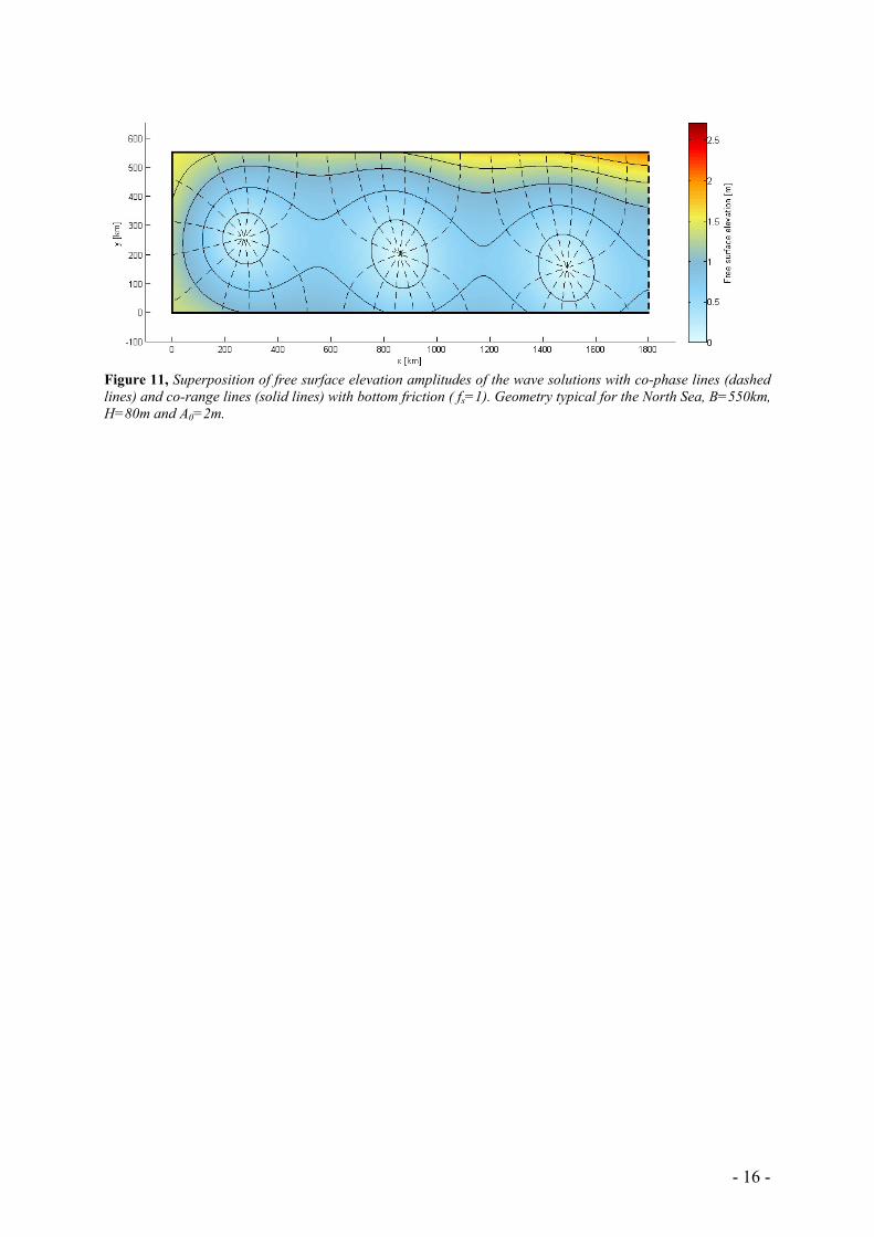
- 16 -
Figure 11, Superposition of free surface elevation amplitudes of the wave solutions with co-phase lines (dashed
lines) and co-range lines (solid lines) with bottom friction ( fs=1). Geometry typical for the North Sea, B=550km,
H=80m and A0=2m.

- 17 -
For this study an extended Taylor (ET-) model is setup, which allows abrupt width- and depth-
changes and one or two open boundaries through which tidal waves can be forced into the
model’s basin. The model is based on the shallow water equations, combined with previous
published literature. In this chapter the model setup is presented.
The solution to (non) frictional Taylor problem in section 3.5 is a superposition of a forced and a
reflected Kelvin wave and an infinity number of Poincaré modes in one semi-enclosed basin. The
model used in this study is an extension to the frictional Taylor problem (Rienecker & Teubner,
1980). It is able to connect several rectangular basins, sub-basins, to represent the depth- and
width-variations in the North Sea. In addition, a second wave may be forced into the system to
represent both the open boundary with the Atlantic Ocean in the North and the Dover Strait. In
the following sections, the model setup is described.
4.1.1. Basin setup
The geometry is built up out of rectangular sub-basins, which are horizontally connected through
an open boundary. The number of rectangular sub-basins is arbitrary. The rectangular sub-basins
may vary in length, width, latitude and uniform depth. In figure 12 a possible basin setup with
3=bN sub-basins is shown, which is used to explain the model further. The lateral boundary at
x=0 may either be closed or open, depending on the problem setup.
Figure 12, setup of the basin with spatial varying compartments, the solid lines are closed boundaries, the wide
dashed lines are open boundaries and the narrow dashed line is either a closed or an open boundary.
Sub-basin one has a length of 21 LLl −= , a width of 1,21,11 BBb −= and a uniform depth of 1H ,
sub-basin two has a length of 122 LLl −= , a width of 2,22,12 BBb −= and a uniform depth 2H
4. Extended Taylor model: abrupt width- and . depth-changes
4.1. Model setup

- 18 -
and sub-basin three has a length of 13 Ll = , a width of 3,23,13 BBb −= and a uniform depth of 3H .
To describe the the lateral displacement between two basins, Dn [m], is defined as
( ) ( )11,1,1 5.0 ++ −+−=bbbb nnnnn bbBBD (20).
Here nb is the basin number. The spatial characteristics, the number of sub-basins and the lateral
displacement are arbitrary, as long as the sub-basins are connected to each other through an open
boundary.
4.1.1.1. Boundary conditions
Each sub-basin may contain three types of boundaries, i.e. longitudinal closed boundaries, lateral
closed boundaries and lateral open boundaries. Through a closed boundary a no flux condition is
demanded. At an open boundary located in between two sub-basins, continuity of normal flux and
continuity of free surface elevation is demanded. For the basin shown in figure 12 the boundary
conditions are
LxL <<2 and 1,1By = or 1,2By =
BC (1.a),
21 LxL << and 2,1By = or 2,2By =
BC (1.b), 0=v for
10 Lx << and 3,1By = or 3,2By =
BC (1.c),
2Lx = and 1,12,1 ByB << or 1,22,2 ByB <<
BC (2.a),
1Lx = and 3,12,1 ByB << or 2,23,2 ByB <<
BC (2.b), 0=u for
If closed at x=0 : 0=x and 3,23,1 ByB <<
BC (2.c),
2211 HuHu = ,
BC (3.a),
21 ζζ =
for 2Lx = and 2,21,1 ByB <<
BC (3.b).
3322 HuHu = ,
BC (4.a),
32 ζζ =
for 1Lx = and 3,23,1 ByB <<
BC (4.b).
If the lateral boundary at x=0 is open, BC (2.c) is omitted. Through an open boundary which is not
located in between two sub-basins (x=L and x=0 if open), a forced Kelvin wave is imposed, while
allowing other wave to freely leave the basin domain.

- 19 -
4.1.2. Linear shallow water equations
The linear shallow water equations are used to simulate the tidal dynamics in the model basins.
Here the linear shallow water equations (5.a-c) as derived in section 3.3 are repeated:
Momentum x-direction x
gH
rufv
t
u
∂∂
−=+−∂∂ ζ
(21.a),
Momentum y-direction y
gH
rvfu
t
v
∂∂
−=++∂∂ ζ
(21.b),
Mass balance 0=
∂∂
+∂∂
+∂∂
y
v
x
uH
t
ζ (21.c).
Its fundamental wave solutions, frictional Kelvin and Poincaré waves, have been presented in
section 3.4.2 and 3.4.3 of the theoretical background chapter.
The wave solution in a sub-basin is the superposition of two Kelvin waves and two families of
Poincaré modes. The arrows in figure 13 are a schematisation of the Kelvin and Poincaré waves.
The problem is forced by one or two Kelvin waves. The Kelvin waves are partly reflected at the
lateral boundaries and partly transmitted through the open lateral boundaries of the sub-basin.
Figure 13, Kelvin and Poincaré waves and collocation points in each sub-basin.
If the lateral boundary at x=0 is closed, the waves (1…M3, 3) are reflected at x=0 into waves
(M3+1…2M3,3). If the lateral boundary at x=0 is open, Kelvin wave (M3+1,3) is a forced, Kelvin
wave (1,3) propagates outside the model boundaries at x=0 and Poincaré waves (M3+2…2M3, 3) no
longer exist.
4.2. Solution method

- 20 -
To solve a defined problem, a truncated set of Poincaré modes and a collocation technique is used.
The dots in figure 13 represent the collocation points. The collocation points are divided into four
groups; lnbcy ,, , collocation points at the left closed boundary in sub-basin nb, rnbcy ,, , collocation
points at the right closed boundary in sub-basin nb, nboy , , collocation points at the open boundary
between sub-basin nb and nb+1 and nbocy , , collocation points at the open-closed boundary in sub-
basin Nb. The number of Poincaré modes in a sub-basin depends on the allocated number of
collocation points at a lateral boundary.
4.2.1. Collocation points
The number of collocation points allocated to a lateral boundary depends on the width of a
boundary and on M1, the number of collocation points allocated at the open and closed boundaries
of sub-basin one. A spacing parameter, c∆ [m], determines the average spacing between the
collocation points, i.e.
1
1
M
bc =∆ (22).
Along the lateral boundary lines of each sub-basin the number of collocation points, Mnb [-], is
determined by dividing the width of a sub-basin, bnb [m] , through c∆ , and rounded to an integer.
∆
=c
broundM nb
nb (23).
Since each sub-basin is a rectangle, the number of collocation points on the left and right lateral
boundary lines is equal in each sub-basin. The number of collocation points on the lateral
boundary lines is again linear divided over the closed and open boundaries, depending on the
length of a boundary. A distinction is made between closed boundaries under an open boundary,
1,1,1 +− nbnb BB and above an open boundaries, 1,2,2 +− nbnb BB .
In the positioning of the collocation points, two groups are distinguished, i.e. closed boundaries
and open boundaries. The collocation points at the closed boundaries have a transverse spacing of
cb NL / . Here bL is the boundary length and cN is the number of collocation points allocated at
the boundary. Closed boundaries under an open boundary have their first collocation point at
nbB ,1 and above an open boundary at nbB ,2 .
The collocation points at the open and open-closed boundaries also have a transverse spacing of
cb NB / . However, the first and last collocation points are located at )/(5.0 cb NL above and under
a closed boundary respectively. Figure 13 shows a visualisation of the deviation of collocation
points.

- 21 -
4.2.2. Linear system
A mathematical problem arises with M1+2M2+aM3 unknown complex amplitudes and
M1+2M2+aM3 independent expressions at the collocation points. Here a is two if the lateral
boundary at x=0 is closed and one if open. The problem can be written as
BC (2.a)
( ) 0)(ˆ)(ˆ),(ˆ)(
11,0
1
)(
11,1,1,
1
1, =+=∑=
xki
cforced
M
n
xki
cncnn eyueyuyxu ,
BC (2.b)
( ) 0)(ˆ),(ˆ2
1,
2
1
)(
22,2, ==∑=
M
n
xki
cncneyuyxu ,
BC (3.a)
( ) ( ) 0)(ˆ)(ˆ)(ˆ),(ˆ2
2,
1
1,
2
1
)(
12,2
)(
11,01
1
)(
11,11, =−+= ∑∑==
M
n
xki
on
xki
oforced
M
n
xki
ononincn eyuHeyuHeyuHyxu ,
BC (3.b)
( ) ( ) 0)(ˆ)(ˆ)(ˆ),(ˆ2
2,
1
1,
2
1
)(
12,
)(
11,0
1
)(
11,1, =−+= ∑∑==
M
n
xki
on
xki
oforced
M
n
xki
ononincn eyeyeyyx ζζζζ ,
If lateral boundary at x=0 is closed:
BC (2.c)
( ) 0)(ˆ),(ˆ3
1,
2
1
)(
22,2, == ∑=
M
n
xki
cncneyuyxu ,
BC (4.a)
( ) ( ) 0)(ˆ)(ˆ),(ˆ3
2,
2
1,
2
1
)(
13,3
2
1
)(
12,22, =−= ∑∑==
M
n
xki
on
M
n
xki
ononn eyuHeyuHyxu ,
BC (4.b)
( ) ( ) 0)(ˆ)(ˆ),(ˆ3
2,
2
1,
2
1
)(
23,
2
1
)(
22,2, =−= ∑∑==
M
n
xki
on
M
n
xki
ononn eyeyyx ζζζ .
If lateral boundary at x=0 is open:
BC (4.a)
( ) ( ) 0)(ˆ)(ˆ)(ˆ),(ˆ)(
13,13
1
)(
13,3
2
1
)(
12,22,
3,13
3
3
2,
2
1, =−−= +
+==∑∑ xki
oMforced
M
n
xki
on
M
n
xki
ono
Mnn eyuHeyuHeyuHyxu ,
BC (4.b)
( ) ( ) 0)(ˆ)(ˆ)(ˆ),(ˆ3
3,13
3
2,
2
1,
1
)(
13,1
)(
23,
2
1
)(
22,2, =−−= ∑∑=
+=
+
M
n
xki
oMforced
xki
on
M
n
xki
ono
Mnn eyeyeyyx ζζζζ .
The different subscripts can be found in figure 13. The solving of the complex amplitudes is done
in Matlab. The forced complex amplitudes contain both an amplitude and a phase.

- 22 -
The coming chapter holds the model results of the tidal dynamics in the North Sea. The results are
in three-fold, i.e. the model results of the M2-, S2-, K1- and O1-tidal constituents (1) compared with
the tidal data, (2) without the Dover Strait and (3) without bottom friction. The chapter starts
with the model basin, the calibration and simulation setup, followed by the presentation of the
results. Four model basins setups of the North Sea were calibrated for the M2-tide to analyze the
effect of basin orientation and geometry detail. The basin setup which showed the best result is
used as further representation of the North Sea in the simulations.
A generic Matlab script was written to fit the model basins on the geometric data and to project
the tidal data on the model boundaries. Two basin orientations were used to fit a model basin, i.e.
aligned to the Southern Bight and aligned to the main basin of the North Sea. For each basin
orientation a simple geometry, consisting of several sub-basins, and a moderately detailed
geometry, consisting of a dozen sub-basins, were generated. The basins are setup in such way, that
they cover the largest geometry variation of the North Sea, i.e. depth, width and length variations.
In each of the four basin setups two open boundaries are situated through which tidal and Kelvin
waves can be forced into and exit the system. They represent the open boundary with the Atlantic
Ocean in the North and the Dover Strait.
A detailed description of the four basins setups can be found in appendix B. The basin setup
“Southern Bight moderately detailed” is shown in figure 14. The letters A. B, C, D and E denote
four parts of the North Sea; i.e. (A-B; west coast) the Scottish and English west coast, (B-C;
Southern Bight) the Southern Bight, (C-D; east coast) the northern part of the Dutch coast, the
German coast and the western part of the Danish coast and (D-E; Norwegian trench) the northern
part of the Danish coast and the Norwegian coast.
Figure 14, basin setup 3, “Southern Bight moderately detailed” with 12 sub-basins. Thick red lines are closed
boundaries and dashed red lines are open boundaries. The small black dots are regular data-station and the
small green dots are regular Norwegian Trench data stations.
5. Tidal dynamics in the North Sea
5.1. Model basin setup

- 23 -
The tidal data is used to calibrate the model for a specific basin setup and tidal constituent, and to
determine the model simulation performance. Four types of tidal stations were distinguished, i.e.
regular, rivers, estuary and islands. Only the tidal stations of type regular are used to calibrate a
tidal constituent, to neglect as much of the local influences on the tide as possible. A distance filter
of 50km is used, which means that tidal stations which decent more than 50km from a closed
model boundary are also neglected. For each basin setup the used tidal data is extracted and
projected on the model boundaries. The generic Matlab script generats a data output which holds
the basin setup (geometries, displacements and latitudes) and the projected tidal data (projected
location, amplitude and phase), and can be loaded and simulated in the ET-model.
For each simulation the tidal constituents are calibrated on the tidal data. Five variables can be
calibrated, i.e. the relative friction coefficient, fs, the amplitude, A0, and phase, 0ϕ , of the tidal
wave entering the North Sea through the northern open boundary with the Atlantic Ocean and
the amplitude, A0d, and phase, d0ϕ , of the tidal wave entering through the Dover Strait. The
model variables fs, A0, 0ϕ and A0d are calibrated by minimizing the scaled averaged squared error
between the amplitudes of the tidal data, dataA , and the simulation, simA , i.e.
( )∑=
−=dN
n
nsimnsim
d
squared AAAN
E1
2
,,2
0*
1 (24).
Here dN is the number of projected data stations and squaredE the scaled average squared error.
The model variable d0ϕ is used to calibrate the tidal phase, not changing the phase difference
between 0ϕ and d0ϕ . For the calibration process a generic simulation loop is written around the
ET-model. The loop is run multiple times, varying the value of the variables and minimizing the
squaredE . In the calibration process of the M2-, S2-, K1- and O1-tidal constituents, the tidal data
stations “regular Norwegian Trench”, denote green in figure 14, were ignored due to the large
lateral depth variations in the North Sea. This is further discussed in section 9.2 of the discussion.
To analyze the impact of basin orientation and basin geometry detail, the basin setups presented in
appendix B were calibrated for the M2-tide. The basin setup “Southern Bight moderately detailed”
showed the best results for the M2-tide, and was used to further analyze the tidal dynamics of the
North Sea. Table 2 contains an overview of the performed calibrations.
Setup Tide Orientation Number of
sub-basins
1 M2 3
2 M2 North Sea
12
3 M2 4
4 M2 Southern Bight
12
5 S2
6 K1
7 O1
Southern Bight 12
Table 2, calibration setup North Sea tide.
5.2. Calibration setup
5.3. Simulation setup

- 24 -
After calibration, all setups were simulated with the calibrated parameters. For the setups 4-7 two
cases were simulated, i.e. (1) no Dover Strait and (2) no bottom friction. In the no Dover Strait
case the lateral open boundary at x=0 is closed, i.e. the Dover Strait is no longer simulated. In the
no bottom friction case fs is set to 0, i.e. the effect of bottom friction is no longer simulated. In
total fifteen simulation were performed. Table 3 contains an overview of the performed
simulations.
Run Tide Basin
orientation
Number of
sub-basins
Bottom
friction
Dover Strait
1 M2 North Sea 3
2 M2 North Sea 12
3 M2 Southern Bight 4
yes
yes
4 M2 Southern Bight 12 yes yes
5 S2
6 K1
7 O1
Southern Bight 12 yes yes
8 M2
9 S2
10 K1
11 O1
Southern Bight 12 no yes
12 M2
13 S2
14 K1
15 O1
Southern Bight 12 yes no
Table 3, simulation setup, i.e. run 1-4 is the basin setups, run 4-7 the results tidal constituents, run 8-11 case no
bottom friction and run 12-15 case no Dover Strait.
As typical tidal amplitude of the amphidromic system, Z (see equation 3), the A0 of the M2-tide
was used for all tidal constituents.
In appendix C.1-4 a detailed overview of the calibration and simulation results of run 1-4 is
presented. In table 4 the scaled averaged squared error and the correlation coefficient, rcorr,
between the tidal amplitude of the data and the simulation are presented.
Setup squaredE rcorr
- -
1 0.069 0.80
2 0.045 0.94
3 0.086 0.79
4 0.036 0.94
Table 4, results calibration M2-tide for basin setup 1-4.
All four basin setups show an M2-amphidromic system with three amphidromic points, as seen in
the North Sea. The moderately detailed geometries, setup 2 and 4, show significant better results
than the simple detailed geometries, setup 1 and 3. The basin setup Southern Bight moderately
5.4. Results basin setups (run 1-4)
- 25 -
detailed does not involve the Skagerrak whereas North Sea moderately detailed does. The
Skagerrak was not involved in the depth calculations of the sub-basins, because it caused a sudden
deep trench along the English coast. Both basin setups showed good results on the tidal ranges of
the M2-tide, neglecting the tidal ranges along the Norwegian Trench. The basin setup North Sea
moderately detailed showed better results on the tidal phase. However, when simulating the K1-
and O1-tide, tidal resonance occurred in the Skagerrak, which is not seen in the tidal data. For this
reason the Southern Bight moderately detailed basin setup is was used as representation of the
North Sea.
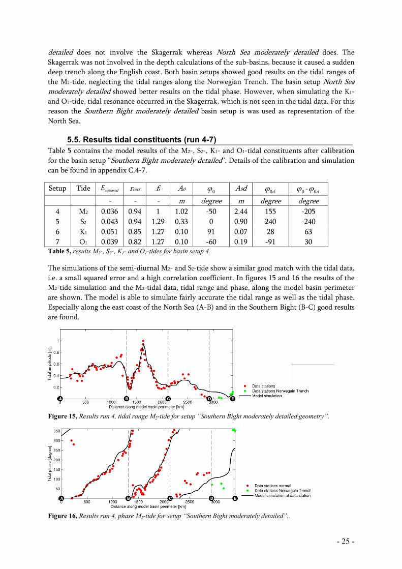
Table 5 contains the model results of the M2-, S2-, K1- and O1-tidal constituents after calibration
for the basin setup “Southern Bight moderately detailed”. Details of the calibration and simulation
can be found in appendix C.4-7.
Setup Tide squaredE rcorr fs A0 0ϕ A0d
d0ϕ 0ϕ - d0ϕ
- - - m degree m degree degree
4 M2 0.036 0.94 1 1.02 -50 2.44 155 -205
5 S2 0.043 0.94 1.29 0.33 0 0.90 240 -240
6 K1 0.051 0.85 1.27 0.10 91 0.07 28 63
7 O1 0.039 0.82 1.27 0.10 -60 0.19 -91 30 Table 5, results M2-, S2-, K1- and O1-tides for basin setup 4.
The simulations of the semi-diurnal M2- and S2-tide show a similar good match with the tidal data,
i.e. a small squared error and a high correlation coefficient. In figures 15 and 16 the results of the
M2-tide simulation and the M2-tidal data, tidal range and phase, along the model basin perimeter
are shown. The model is able to simulate fairly accurate the tidal range as well as the tidal phase.
Especially along the east coast of the North Sea (A-B) and in the Southern Bight (B-C) good results
are found.
Figure 15, Results run 4, tidal range M2-tide for setup “Southern Bight moderately detailed geometry”.
Figure 16, Results run 4, phase M2-tide for setup “Southern Bight moderately detailed”..
5.5. Results tidal constituents (run 4-7)

- 26 -
In figure 17 and 18 the simulated and the measured amphidromic system of the M2-tide are
shown. The two figures show very similar patterns, which confirms the good model results along
the perimeter presented in figures 15 and 16.
Also for the diurnal K1- and O1-tide a similar and good match with the tidal data is found. The
results of the K1-tide are shown in figures 19 and 20. Best results are again found along the east
coast of the North Sea (A-B) and in the Southern Bight (B-C).
Figure 19, Results run 4, tidal range K1-tide for setup “Southern Bight moderately detailed geometry”.
Figure 20, Results run 4, phase K1-tide for setup “Southern Bight moderately detailed”..
Figure Figure Figure Figure 17171717.... Model simulation result of the M2-
amphidromic system. Dashed lines are co-phase lines,
normal lines co-range lines.
Figure 18, Amphidromic system of the M2-tide in
the North Sea (Dyke 2007). The solid lines are the
co-phase lines and the dashed lines are the co-
range lines.

- 27 -
The model results of the no bottom friction and the no Dover Strait case for the M2-, S2-, K1- and
O1-tidal ranges are presented in figure 21 to 24. In the figures the black line represents the model
results after calibration on the tidal data (run 4-7), the blue line represents the no bottom friction
case and the red line the no Dover Strait case.
For the semi-diurnal M2- and S2-tide similar effects are seen in the two cases. The bottom friction
mainly damps the tidal ranges, except near the Scottish coast (A-500km), were bottom friction
increases the tidal ranges. The relative effect of the bottom friction increases along the perimeter,
with an absolute maximum along the west coast (B-C). The effect of the Dover Strait on the M2-
and S2-tide is small along the east coast (A-B). In the Southern Bight (B-C) the effect of the Dover
Strait is strong, increasing the tidal ranges. Also along the west coast (C-D) and the Norwegian
trench (D-E) an increase in tidal ranges is seen due to the Dover Strait, which implies that the
Dover Strait is a source of tidal energy for the M2- and S2-tide.
Figure 21, Results of the M2-tide no bottom friction and no Dover Strait case.
Figure 22, Results of the S2-tide no bottom friction and no Dover Strait case.
Also the diurnal K1- and O1-tide show a similar pattern for both cases. The bottom friction damps
the tidal ranges. The effect increases along the perimeter, with a relative and an absolute
maximum in the Southern Bight (B-C). The Dover Strait has a negligible effect on the tidal ranges
along the west coast (A-B). In the Southern Bight (B-C) the Dover Strait causes a decrease in tidal
range. The decrease is probably caused by an elevation amphidromic point present in the Dover
Strait, which does not develop in the absence of the Dover Strait. Along the west coast (C-D) and
in the Norwegian Trench (D-E) the Dover Strait imposes an increase in tidal ranges, which implies
that the Dover Strait is a source of tidal energy.
5.6. Results no bottom friction (run 8-11) and no Dover Strait (run 12-15)

- 28 -
Figure 23, Results of the K1-tide no bottom friction and no Dover Strait case.
Figure 24, Results of the O1-tide no bottom friction and no Dover Strait case.

- 29 -
The coming chapter contains the setup and results of the physical mechanisms of tidal resonance
in the Southern Bight. By varying the simulation setup, the effect of basin geometry, friction and
rotation on tidal resonance is analyzed. A total of 13 resonance simulations were performed. The
chapter starts with a description of the problem setup and the results are presented afterwards.
To analyze tidal resonance, the ET-model as described in chapter 3 is used with a two basin setup,
as shown in figure 25. In the figure the wide dashed lines are open boundaries, the solid lines are
closed boundaries and the small dashed line is either a closed, open or partly closed/partly open
boundary, depending on the setup.
Figure 25, tidal resonance setup; two sub-basins.
A generic resonance-loop was written around the ET-model, which runs the defined problem
setup multiple times, analyzing the tidal ranges in sub-basin two, when varying the length and
width of sub-basin two and keeping all other variables constant. For each run two types of results
are calculated; (Aclosed) the average tidal range at the closed end of sub-basin two and (Aaveraged) the
average tidal range over sub-basin two. As a result, a resonance map is created, which plots a
resonance factor versus the geometry of sub-basin two. Two tidal resonance factors are defined,
which quantify the scaled tidal ranges in sub-basin two, i.e.
scaled average tidal range at x=0 and B1,2<y< B2,2; 0/ AAF closedc = (25),
scaled average tidal range over sub-basin two; 0/ AAF averagea = (26).
Here A0 is the amplitude of the forced Kelvin wave in sub-basin one at x=L1. A resonance map is
created by plotting a resonance factor versus the scaled width, b2/L02, and the scaled length, l2/L02.
Here L02 is the Kelvin wave length in sub-basin two.
6. Tidal resonance; physical mechanisms
6.1. Basin setup

- 30 -
Five setup types were simulated and compared with a reference run to analyse the effect of basin
geometry, friction and rotation on tidal resonance. In each setup type one certain aspect is varied
from the reference run. The geometry of sub-basin one is kept constant for all runs, b1=550km,
l1=800km and H1=80m, typical values for the main basin of the North Sea. For the reference run
the system is forced with a Kelvin wave at x = L with a period of 12:25hour and an amplitude of
20 =A m at x = L1, typical for the M2-tide in the North Sea. The geometry of sub-basin two is
based on the Southern Bight, with a typical depth of H2=25m. A typical latitude of 55⁰N is used for
both basins.
The setup of the simulations is shown in table 6. In run 3.1, the top of sub-basin one and two are
aligned, i.e. B2.1 = B2.2, in simulation 3.2 the bottoms are aligned, i.e. B1.1 = B1.2. In the simulations
6.1- 6.4 the lateral boundary at x=0 is (partly) open. The setup of these runs is further specified in
section 6.5.
Simulation type No l2 b2 H2 D1 Lat fs x=0
- km km m km ⁰N -
Reference 1 0-1050 10-550 25 0 55 0 Closed
Basin depth 2.1 ” ” 40 ” ” ” ”
2.2 ” ” 80 ” ” ” ”
Displacement 3.1 ” ” ” top ” ” ”
3.2 ” ” ” bottom ” ” ”
Rotation 4.1 ” ” ” ” 0.001 ” ”
4.2 ” ” ” ” 89 ”
Friction 5.1 ” ” ” ” ” 0.2 ”
5.2 ” ” ” ” ” 1 ”
Open boundary 6.1-2 ” ” ” ” ” ” Open
6.3-4 ” ” ” ” ” ” Partly open Table 6, simulation setup tidal resonance, the value ” means similar to reference run.
For simulation runs 2-5, Fc is used as tidal resonance factor, as the highest tidal ranges due to
resonance are found at the lateral boundary at x=0. However, for simulation runs 6.1- 6.4 this is no
longer valid, and Fa is used as resonance factor. For the reference run all resonance factors are
shown in a resonance map. The sections 5.3, 5.4 and 5.5 contain the results of the reference run,
geometry, rotation and friction and second open boundary respectively. In section 5.6 a written
summary of the results is given.
This section contains the results of the reference run. Figures 26 and 27 show the resonance maps
of Fc and Fa respectively. The figures show a comparable pattern. For small widths, the quarter and
three-quarter Kelvin wave length resonance is clearly visible (red peaks). With increasing width
the intensity of the resonance peaks fades, and the resonance peaks which are ≥0.75 l2/L02 are
found at smaller basin lengths, seen as a leftwards bending of the peaks in the figures. The first
quarter wave length resonance peak stays centred around 0.25 l2/L02..
6.2. Simulation setup
6.3. Results reference run

- 31 -
Figure 26, resonance map run 1; Fc as function of the
scaled geometry of sub-basin one.
Figure 27, resonance map run 1; Fa as function of the
scaled geometry of sub-basin one.
Figures 28 and 29 contain the results of the depth variations, run 2.1 and 2.2 respectively. For both
runs the depth in sub-basin two is increased, resulting in longer Kelvin wave lengths, L02, and thus
less resonance peaks for the same basin length domain (0-1050km). The intensity of the quarter
and three-quarter resonance peaks fades faster the closer the factor H1/H2 is to one, equal depth in
sub-basin one and two.
Figure 28, results run 2.1, H2= 40m; Fc as function of
the scaled geometry of sub-basin one.
Figure 29, results run 2.2, H1= H2= 40m; Fc as
function of the scaled geometry of sub-basin one.
In figures 30 and 31 the results of the lateral displacement, run 3.1 and 3.2, are presented. The
results show a slightly different pattern from the reference run.
Figure 30, results run 3.1, lateral displacement top;
Fc as function of the scaled geometry of sub-basin
one.
Figure 31, results run 3.2, lateral displacement
bottom; Fc as function of the scaled geometry of sub-
basin one.
The results of the runs 4.1 and 4.2, rotation, are presented in the figures 32 and 33 respectively.
Both runs show the quarter and three-quarter Kelvin wave length resonance peaks for small basin
widths. In case of negligible rotation, run 4.1, the position of a resonance peak is not influenced by
the basin width. In case of rotation, run 4,2, the resonance peaks which are ≥0.75 l2/L02 tend to
resonate at smaller basin lengths with increasing width. In the case of negligible rotation the
resonance peaks are much more intensive than in the case with rotation.
6.4. Results geometry, rotation and friction

- 32 -
Figure 32, results run 4.1, latitude= 0.001⁰N; Fc as
function of the scaled geometry of sub-basin one.
Figure 33, results run 4.2, latitude= 89⁰N; Fc as
function of the scaled geometry of sub-basin one.
Figures 34 and 35 contain the results of run 5.1 and 5.1, friction, respectively. For increasing
friction, the resonance peaks fade with increasing width and length, i.e. travel length of the wave.
Friction also causes a slight decrease in the Kelvin wave length.
Figure 34, results run 5.1, fs=0.2; Fc as function of
the scaled geometry of sub-basin one.
Figure 35, results run 5.2, fs=1; Fc as function of the
scaled geometry of sub-basin one.
For the runs 6.1 and 6.2 the lateral boundary at x=0 is open, which means bopen = b2. Here, bopen is
the width of the second open boundary. For the runs 6.3 and 6.4 the lateral boundary at x=0 is
partly open, bopen =0.5b1 and bopen =0.25b1 respectively. The lateral displacement between sub-basin
two and the partly open boundaries is set to zero (see equation 20 for lateral displacement). A
second tidal wave is forced into the system through the second open boundary, with an amplitude
A0d and a phase d0ϕ . Table 7 contains the setup details of the second forced Kelvin wave.
Run bopen D A0d d0ϕ
km m m
6.1 b2 - A0 0
6.2 b2 - A0 90
6.3 0.5b2 0 A0 0
6.4 0.25b2 0 A0 0 Table 7, details setup second open boundary
In figures 36 and 37 the results of run 6.1 and 6.2 are shown. The resonance patterns seen on both
figures are the same, whereas the phase difference shifts the locations of the peaks. The quarter
and three-quarter Kelvin wave length resonance patterns are no longer seen. Instead a spacing of
0.75 l2/L02 is seen.
6.5. Results second open boundary
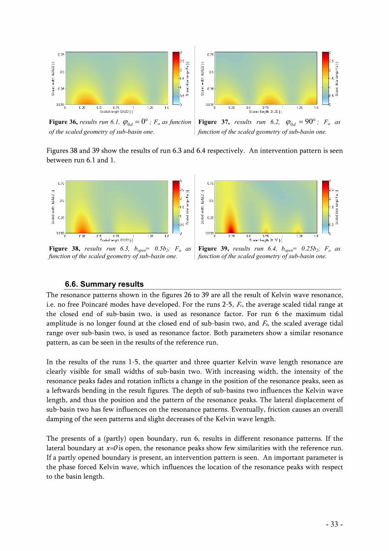
- 33 -
Figure 36, results run 6.1, °= 00dϕ ; Fa as function
of the scaled geometry of sub-basin one.
Figure 37, results run 6.2, °= 900dϕ ; Fa as
function of the scaled geometry of sub-basin one.
Figures 38 and 39 show the results of run 6.3 and 6.4 respectively. An intervention pattern is seen
between run 6.1 and 1.
Figure 38, results run 6.3, bopen= 0.5b2; Fa as
function of the scaled geometry of sub-basin one.
Figure 39, results run 6.4, bopen= 0.25b2; Fa as
function of the scaled geometry of sub-basin one.
The resonance patterns shown in the figures 26 to 39 are all the result of Kelvin wave resonance,
i.e. no free Poincaré modes have developed. For the runs 2-5, Fc, the average scaled tidal range at
the closed end of sub-basin two, is used as resonance factor. For run 6 the maximum tidal
amplitude is no longer found at the closed end of sub-basin two, and Fa, the scaled average tidal
range over sub-basin two, is used as resonance factor. Both parameters show a similar resonance
pattern, as can be seen in the results of the reference run.
In the results of the runs 1-5, the quarter and three quarter Kelvin wave length resonance are
clearly visible for small widths of sub-basin two. With increasing width, the intensity of the
resonance peaks fades and rotation inflicts a change in the position of the resonance peaks, seen as
a leftwards bending in the result figures. The depth of sub-basins two influences the Kelvin wave
length, and thus the position and the pattern of the resonance peaks. The lateral displacement of
sub-basin two has few influences on the resonance patterns. Eventually, friction causes an overall
damping of the seen patterns and slight decreases of the Kelvin wave length.
The presents of a (partly) open boundary, run 6, results in different resonance patterns. If the
lateral boundary at x=0 is open, the resonance peaks show few similarities with the reference run.
If a partly opened boundary is present, an intervention pattern is seen. An important parameter is
the phase forced Kelvin wave, which influences the location of the resonance peaks with respect
to the basin length.
6.6. Summary results

- 34 -
In the coming chapter the results of tidal resonance in the Southern Bight are presented. By
varying the depth in the Southern Bight, the state of resonance of the M2-, S2 -, O1- and K1-tide in
the Southern Bight is analyzed. The chapter starts with a setup of the problem, thereafter the
results are presented.
The basin setup “Southern Bight moderately detailed” as shown in figure 40 is used as
representation of the North Sea; see Appendix B-4 for details of the basin setup. The sub-basins 9
to 12, highlighted yellow in figure 40, represent the Southern Bight.
Figure 40, basin setup “Southern Bight moderately detailed”. The yellow area represents the Southern Bight.
The tide in the Southern Bight is represented by the scaled average tidal range over sub-basins 9 to
12, i.e.
nn
n
naverage
n
nn
a lbA
lbA
F ∑∑ =
=
=12
9
,12
9
0
1
(27).
See section 6.1 for an explanation of used variables. A total of four simulations were performed. By
varying the depth in the Southern Bight, resonance charts are created which plot the depth in the
Southern Bight versus Fa. Table 8 show the setup of the two runs. In the table ∆Hsb is the percental
depth in sub-basin 9-12 of the original depth as shown in appendix B-4. The value of the variables
A0, A0d, 0ϕ and d0ϕ were used as calibrated in chapter 5. Each setup is run with and without
bottom friction to show possible damped resonance patterns.
Setup Constituent T ∆Hsb fs A0 0ϕ A0d
d0ϕ
- - hour % - m m
1 M2 12:25 2-200 1 1.02 -50 2.44 192
2 S2 12:00 2-200 1.29 0.29 0 0.59 272
3 K1 23:57 2-200 1.27 0.10 91 0.07 28
4 O1 25:49 2-200 1.27 0.10 -60 0.19 -91 Table 8, Simulation setup tidal resonance Southern Bight
7. Tidal resonance; Southern Bight
7.1. Setup tidal resonance in Southern Bight

- 35 -
In the figures 41 to 44 the results of the simulation are shown in resonance charts. The red lines
show the simulations with bottom friction and the dashed black line without bottom friction.
None of the M2-, S2 -, O1- and K1-tidal constituents is currently in a state of resonance. In the case
of no bottom friction resonance would occur for depth smaller than 10m. When including bottom
friction, the seen resonance patterns are no longer visible.
Figure 41, Resonant chart M2-tide, simulation 1; the
red line is with bottom friction and the dashed black
line without bottom friction. .
Figure 42, Resonant chart S2-tide, simulation 2; the
red line is with bottom friction and the dashed black
line without bottom friction. .
Figure 43, Resonant chart K1-tide, simulation 3; the
red line is with bottom friction and the dashed black
line without bottom friction. .
Figure 44, Resonant chart O1-tide, simulation 4; the
red line is with bottom friction and the dashed black
line without bottom friction. .
7.2. Results tidal resonance in Southern Bight

- 36 -
The results of the case study to a giant scale windmill park situated in the Southern Bight are
presented in the coming chapter. The chapter starts with the problem setup, after which the
results are presented.
Two model cases are simulated, i.e. a windmill park which covers a minor and a windmill park
which covers a major area of the Southern Bight. The basin setup “Southern Bight moderately
detailed” as shown in figure 45 and figure 46 are used as representation of the North Sea. The
green hatched areas represent the locations of the windmill parks.
To represent the windmill parks in the model simulations, the friction is increased in the green
hatched areas. Van der Veen (2008) estimated, that the drag coefficient imposed by a windmill
park, Cd_wt, is in the order of 0.4*10-6 - 0.4*10-4. Compared with the Cd as used for the bottom
friction, see equation (2), this implies an increase in bottom friction in the order of 0.02-2%. In
the simulation the most extreme case is simulated, i.e. a 2% increase in bottom friction at the
location of the windmill parks. The M2-tidal constituent is used as representation of the tide in
the North Sea, as it is the largest tidal constituent. The values of tidal variables are used as
calibrated in chapter 5. In table 9 the setup of the two simulated cases is shown.
Setup Coverage Constituent T fs A0 0ϕ A0d
d0ϕ
hour - m degree m degree
1 minor M2 12:25 1-1.02 1.02 -50 2.44 192
2 major M2 12:25 1-1.02 1.02 -50 2.44 192 Table 9, Simulation setup tidal windmill park. Southern Bight
8. Windmill park; Southern Bight
8.1. Setup windmill park in the Southern Bight
Figure 45, windmill park with minor
coverage (green area), i.e. sub-basin 10.
Figure 46, windmill park with major coverage
(green area), i.e. sub-basins 9-11.

- 37 -
In the figures 45 and 46 the change in tidal range is shown due to an increase in bottom friction
caused by the windmill parks. For both cases a similar pattern is seen, i.e. west of the elevation
amphidromic points the tidal ranges increase, whereas at all other places a decrease in tidal range
is found. The largest changes are found along the Dutch coast of the Southern Bight and along the
German coast. The changes in tidal range lay in the order of +2mm to -5mm for the minor and
+4mm to -12mm for the major windmill park
Figure 47, Results windmill park minor
coverage. The figure shows the change in tidal
ranges in the North Sea.
Figure 48, Results windmill park major
coverage. The figure shows the change in tidal
ranges in the North Sea.
8.2. Results windmill park in the Southern Bight

- 38 -
An extended Taylor (ET-) model was setup and used to analyze the tidal dynamics of the North
Sea, and in particular the effect of bottom friction and the Dover Strait on the tidal ranges in the
North Sea and tidal resonance in the Southern Bight. In addition, a case study was performed to
the effects of a giant scale windmill park in the Southern Bight. The model is based on Taylor’s
(1920) model with extensions of Rienecker & Teubner (1980), linear friction coefficient, and of
Godin (1965), box schematised geometries. The model solves the tidal dynamics in each sub-basin
as a superposition of an incoming and a reflected Kelvin wave and two truncated families of
Poincaré waves by using a collocation technique. The Kelvin and Poincaré waves are derived from
the shallow water equations, neglecting viscous forces, non linearity and direct tidal forcing. In
the coming chapter the tidal results and the simplification of the ET-model are discussed.
The ET-model was used to simulate the tidal ranges of the M2-, S2-, K1- and O1-tidal constituents
in the North Sea for various simulation setups. The computation time of a simulation lays in the
order of 1sec - 10sec, which made the model ideal to study the physical mechanisms of the North
Sea tide. The collocation technique used to solve the complex wave amplitudes introduced an
energy computation error, i.e. the percental difference between the tidal energy forced into and
leaving the model boundaries in a non-frictional case. The energy computation error lays in the
order of 0 - 5%. The order of this error is roughly a function of the number of collocation points.
On average, 50 collocation points were allocated to a lateral boundary. More collocation points
would decrease the simulation error, however quadratically increase the simulation time.
9.1.1. Model basin
The ET-model is able to solve basin geometries which consist of rectangular sub-basins of uniform
depth, all aligned and connected through an open boundary. The effect of geometry detail, i.e.
number of sub-basins, and basin orientation was analyzed by using four basin setups, which were
all calibrated on the M2-tidal data. All four basin setups are able to generate an amphidromic
system with 3 elevation amphidromic points, as seen in the M2-amphidromic system in the North
Sea. However, the moderately detailed basin setups showed significant better results than the
simple geometries. With the current model setup it is not possible to model the tide in the deep
Skagerrak, because the model does not allow lateral depth variations in the sub-basins. For this
reason the model basin Southern Bight moderately detailed, which excludes the Skagerrak, was
used as representation of the North Sea.
9.1.2. Reproduction of the tidal dynamics in the North Sea
The model was well able to simulate the M2-, S2-, K1- and O1-tidal ranges along the coast of the
North Sea, as well as the effects of specific cases on the tidal ranges. It has to be noted, that the
model does not involve non-tidal meteorological residuals like wind and barometric pressure.
Pugh (1996) estimated, that the standard deviation of the meteorological residuals at four
representative sites in the Southern Bight is 0.23, and thus has a great influence on the actual seen
tidal ranges. The model simulations of the M2-, S2-, K1- and O1-tidal phase in the basin setup
Southern Bight moderately detailed showed good results along the west coast and the Southern
Bight (A-C). However, a structural error along the east coast (C-E) is seen, underestimating the
9. Discussion
9.1. Results ET-model

- 39 -
tidal phase. This might be caused by the Skagerrak, as the phase error is not seen in the M2-model
simulation in the basin setup North Sea moderately detailed, which does involve the Skagerrak.
To simulated the tidal dynamics in the North Sea, five variables were calibrated, i.e. the relative
friction coefficient, fs, and the amplitude and phase of the forced Kelvin waves. It was found that
the minor tidal constituents, S2, K1 and O1, experience more bottom friction than the M2-tide. This
confirms the conclusions of Inoue & Garrett (2007), who showed, that minor tidal constituents
experience up to 50% more friction, i.e. a higher value of fs up to 1.5 for minor tidal constituents.
9.1.3. Tidal resonance in the Southern Bight
The tidal resonance in the Southern Bight has been analyzed in two fold, i.e. (1) the physical
mechanisms of tidal resonance in the Southern Bight and (2) a case study to resonance in the
Southern Bight. The results of the case study show, that M2-, S2-, K1- and O1-tidal constituents are
currently not in a state of resonance. To impose tidal resonance for a non-frictional case in the
Southern Bight, a minimal average depth of 10m is required, where the Southern Bight has a
current average depth of 25m. For the frictional case the resonance peaks are not visible, as they
are damped by the bottom friction. And thus it can be stated, that the Southern Bight is not
sensitive to tidal resonance with respect to geometry changes.
An important factor on tidal resonance in the Southern Bight is the phase difference between the
tidal waves entering the Southern Bight through (1) the Dover Strait and from (2) the northern
boundary with the North Atlantic Ocean. In the no Dover Strait cases it was seen that the Dover
Strait is of importance concerning the tide in the Southern Bight. From the Open Strait results,
run 6.1-2 chapter six, it was seen that the phase difference between the two forced Kelvin waves,
d00 ϕϕ − , is of major importance concerning the resonance patterns. The phase difference
between the two tidal waves entering the Southern Bight is not so likely to change. However, one
should pay attention to it when analyzing the tidal resonance in the Southern Bight.
9.1.4. Windmill park in the Southern Bight
The impact of a giant scale windmill park in the Southern Bight was simulated in two cases by
locally increasing the bottom friction. The increase in bottom friction was based on van der Veen‘s
(2008) work. The simulations show minor changes in the tidal ranges in the Southern Bight and
along the German coast. Note, that only the direct changes in tidal range due to an overall
increase in bottom friction are simulated. Indirect changes in the morphology, which will also
influence the tidal ranges, are not simulated.
Several simplifications were made in the ET-model, which can be classified into two categories,
i.e. (1) geometry simplifications and (2) conservation law simplifications. The ET-model uses
simplified box-schematised geometries of the North Sea, in which lateral depth variations cannot
be involved. In the simplified model basins large lateral geometry variations like the Dogger Bank
and the Norwegian Trench and local geometries variations like rivers and estuaries cannot be
simulated. To avoid simulation errors, only regular tidal stations were used, i.e. few influence of
local geometries, and the tidal stations along the Norwegian Trench were neglected.
The linear shallow water equations were used as conservation laws, i.e. conservation of
momentum and mass. They are a depth-integrated linear form of the Navier-Stokes equations.
One tidal energy dissipation term is present, i.e. linear bottom friction. The horizontal viscosity
9.2. Simplifications of the ET-model

- 40 -
(Roos & Schuttelaars, 2009) and vertical viscosity (Appendix A) terms were neglected, as the
North Sea tide is rather dominated by bottom friction than by viscous forces. The tide generating
forces were also neglected, as the tides in the North Sea is a co-oscillating response to the tides
generated in the North Atlantic Ocean (Banner et al. 1979). To compensate for the simplifications,
the relative friction coefficient, fs, was introduced and calibrated on the tidal data. The calibration
of the friction coefficient can be discussed, as the error introduced by the simplification of the
tidal energy terms is now shaded.
The Southern Bight is most sensitive to non linearity and three-dimensional flow effects, as it is
the most shallow part of the North Sea and large tidal current are present. Good results were
found in the Southern Bight, which implies that the made simplifications are reasonably valid.

- 41 -
The tidal dynamics in the North Sea were studied in an extended Taylor (ET-) model. The model
showed overall good results on the tidal ranges and phases of the M2-, S2-, K1- and O1-tidal
constituents. Several cases were simulated to further analyze the tidal dynamics of the North Sea.
In the coming section all research questions are structurally answered.
(1.1)(1.1)(1.1)(1.1) How can the geometry variations of the North Sea be implemented in a process-based
idealized Taylor model?
The ET-model uses box-schematised model basins,
which consist of rectangular sub-basins of uniform
depth (Godin, 1965). Several model basin were fit on
the geometry of the North Sea. Boundary condition
are a no-normal flow through the closed boundaries
and a continuity of flux and free surface elevation at
the lateral open boundaries between the sub-basins.
A system of linear equation appeared, which was
solved using a collocation technique. In figure 49 the
representative model basin for the North Sea is
shown, consisting of twelve sub-basins. The solid
lines denote the closed boundaries, the dashed red
lines the open boundaries and the letters perimeter
coordinates.
(1.2)(1.2)(1.2)(1.2) How can the Dover Strait be implemented in a process-based idealized Taylor model?
The model allows one or two open boundaries through which Kelvin waves may be forced into
the model basin, while allowing other waves to freely leave the model basin domain. Both the
northern boundary with the Atlantic Ocean as well as the Dover Strait can be simulated, by
forcing two Kelvin waves into the model domain.
(2.1) (2.1) (2.1) (2.1) How well can the model reproduce the observed tidal elevation amplitude and phase along
the coastline of the North Sea?
The M2-, S2-, K1- and O1-tidal constituents were simulated in the representative model basin of the
North Sea, shown in figure 49. The model showed accurate results with respect to the tidal ranges.
Likewise accurate prediction of the tidal phase along the west coast of the North Sea (A-B) and in
the Southern Bight (B-C) were found. Along the east coast and the Norwegian Trench (C-E) a
structural error in the tidal phase was found for all tidal constituents. This is possibly caused by
the absence of the Skagerrak in the representative model basin.
(2.2)(2.2)(2.2)(2.2) Case: how do bottom friction and the Dover Strait influence the tidal ranges in the North Sea?
Two cases were simulated for the M2-, S2-, K1- and O1-tidal constituents, i.e. a no bottom friction
case and a no Dover Strait case. It was found that bottom friction mainly reduces the tidal ranges.
The relative effect of bottom friction increases anti clock-wise along the basin perimeter, from A-
E. The M2- and S2-tide experience an absolute maximum effect of bottom friction along the east
coast (C-D) and the K1- and O1-tide in the Southern Bight (B-C). Further it was found, that the
10. Conclusions and recommendations
Figure 49, representative model
basin of the North Sea consisting of
twelve sub-basins..

- 42 -
Dover Strait acts as a source of tidal energy and increases the tidal ranges along the east coast (C-
E). The Dover Strait amplifies the tidal ranges of the M2-, S2-tide in the Southern Bight, whereas
the K1- and O1-tidal ranges are reduced.
(2.3)(2.3)(2.3)(2.3) What are the physical mechanisms of tidal resonance in the Southern Bight with respect
to basin geometry, rotation, friction and an open Strait (of Dover)?
The physical mechanisms of tidal resonance in the Southern Bight were analyzed in five
simulations runs and one reference run. In the simulation no free Poincaré waves developed, thus
all seen resonance patterns were caused by Kelvin wave resonance. The conclusions regarding the
physical mechanisms of tidal resonance are the following:
Basin depth: Influences the Kelvin wave length, the shape of the
resonance peaks with increasing width and the dissipation
of energy due to friction.
Basin length: Mainly determines whether a system will experiences tidal
resonance, dependent on the Kelvin wave length, i.e.
quarter and three-quarter basin wave length resonance.
Basin width & Rotation: For increasing basin widths, in combination with rotation,
the system tends to resonate at smaller basin lengths than
the quarter and three- quarter basin wave lengths.
Friction: Damps the resonance peaks, and slightly decreases the
Kelvin wave length.
Open Strait (of Dover): A possible major factor on tidal resonance, changing the
shape and dimension of the resonance patterns.
(2.4)(2.4)(2.4)(2.4) Case: is the tide in Southern Bight close to a state of resonance and which depths are needed
to impose tidal resonance?
By varying the average depth in the Southern Bight, the state of resonance of the M2-, S2-, K1- and
O1-tidal constituents was analyzed. It was found that none of the tidal constituent is currently in a
state of resonance and that the tide in the Southern Bight is not sensitive to geometry variations
with respect to tidal resonance.
(2.5)(2.5)(2.5)(2.5) Case: what are the effects of a giant-scale windmill park in the Southern Bight on the
tidal ranges in the North Sea, represented by an increase of the bottom friction?
Two cases were performed, simulating two setups of a giant scale windmill park in the Southern
Bight, represented by an average 2% increase in the bottom friction. It was found that the
simulated windmill parks cause minor direct change in the tidal range in the order of millimetres.
Largest changes were found in the Southern Bight and along the German coast.
Despite the simplifications, the ET-model showed good results simulating the M2-, S2-, K1- and O1-
tidal ranges and phase. Within this study it was shown, that idealised models are, next to studying
a single physical mechanism, well capable of studying a whole amphidromic system. An
interesting topic is the combined use of idealised models and numerical models. Numerical models
use, contrary to idealised models, long computation time. This fact makes them unsuitable for
explorative studies. However, numerical models are well capable of simulating complicated
geometries and non linearity. Where, for example, an idealised model could be used to determine
10.1. Recommendations and future research

- 43 -
the modelling domain and the dominant processes, a numerical model could be used for the
detailed simulations. This could improve computation time and results.
A shortcoming in the ET-model is that the basin setups cannot involve lateral depth variations. De
Boer (2009) and Roos & Schuttelaars (accepted) studied the tidal dynamics using a Taylor model
which allowed lateral depth variations. De Boer solved the Taylor problem for several depth
profiles. The computation time lays in the order of 10min for a semi-enclosed rectangular basin.
Roos & Schuttelaars set up a Taylor model which allowed abrupt lateral and longitudinal depth
steps in a semi-enclosed rectangular basin. This method uses a computation time in the order of
20sec. Involving lateral depth variations in the ET-model described in this study could increase
the performance of the model. The method used by Roos & Schuttelaars would be most suitable to
maintain the idealised character of the model.
In this study, the tidal dynamics are represented by the tidal range, as the tidal range mainly
determines the coastal safety and as relevant data is available and gives a good representation of an
amphidromic system. However, morphological processes are mainly dominated by the tidal
currents. The ET-model could well be used to study the tidal currents in the North Sea or
elsewhere.
The study to the physical mechanisms showed that rotation in combination with increasing basin
width plays an important role on tidal resonance. Many studies to tidal resonance neglect rotation,
so that an analytical solution of the resonance problem can be found. This study could be used as a
basis to setup a new scaling for tidal resonance including rotation.

- 44 -
Banner, F.T., Collins, K. & Massie K.S. (1979) The North-West European shelf seas. Amsterdam:
Elsevier Noord-Holland.
British Admiralty (2010) Admiralty tide tables, volume 1&2. Published by the United Kingdom
hydrographic office.
Brown, T. (1987) Kelvin wave reflection at an oscillating boundary with application to the North
Sea. Continental Shelf Research, Vol. 7, pp. 351-365.
Brown, T. (1989) On a general problem of Kelvin wave reflection at an oscillating boundary.
Continental Shelf Research. Vol 9, pp 931-937.
Carbajal, N. (1997) Two applications of Taylor’s problem for finite rectangular semi-enclosed
basins. Continental Shelf Research, Vol. 17, pp. 803-917.
Carbajal, N., Piney, S. & Rivera, J. G. (2005) A numerical study on the influence of geometry on
the formation of sandbanks. Ocean dynamics, Vol 55, pp. 559-568.
De Boer, W. P. (2009) The influence of lateral depth variations on tidal dynamics in semi-enclosed
basins. Master thesis University of Twente. Retrevied from http://www.wem.ctw.utwente.nl/
onderwijs/afstuderen/afstudeerverslagen/2009/boer.pdf
Dyke, P. (2007) Modeling coastal and offshore processes. London: Imperial college press.
Garrett, C. (1972) Tidal Resonance in the Bay of Fundy and Gulf of Maine. Nature, Vol. 238, pp
441-443.
Garrett, C. (1975) Tides in gulfs. Deep-Sea research. Vol 22, pp 23-35.
Godin, G. (1965) The M2 tide in the Labrador Sea, Davis Strait and Baffin Bay. Deep-Sea Research.
Vol. 12, pp. 469-477.
Godin, G. (1991) On tidal resonance. Continental shelf research. Vol 13, pp 89-107
Hendershott, M.C. & Speranza, A. (1971) Co-oscillating tides in long, narrow bays; the Taylor
problem revisited. Deep-Sea Research. Vol 18, pp 959-980.
Huthnance, J.M. (1991) Physical oceanography of the North Sea. Ocean & Shoreline Management,
Vol 16, pp. 199-231.
Inoue, R. & Garrett, C. (2007) Fourier representation of quadratic friction. Journal of Phys.
Oceanography, Vol. 37, pp 593-610.
11. References

- 45 -
Otto, L., Zimmerman, J.T.E., Furnes, G.K., Mork, M., Saetre, R. & Becker, G. (1990) Review of the
physical oceanography of the North Sea. Netherlands Journal of Sea Research, Vol 26, pp 161-238.
Pedlosky, J. (1982) Geophysical Fluid Dynamics. Springer
Pugh, D. T. (1996) Tides, Surges and Mean Sea-Level. Chippenham ,Wiltshire: Antony Rowe Ltd.
Rienecker , M. N. & Teubner, M.S. (1980) A note on frictional effects in Taylor’s problem. Journal
of Marine Research, Vol. 38, pp 183-191.
Roos, P.C. & Schuttelaars, H.M. (2009) Horizontally viscous effects in a tidal basin: extending
Taylor’s problem. Journal of Fluid Mechanics, Vol, 640, pp. 421-439.
Roos, P.C. & Schuttelaars, H.M. “Influence of topography on tide propagation and dissipation in
semi-enclosed basins”, accepted by Ocean Dynamics.
Sutherland, G., Garrett, C. & Foreman, M. (2005) Tidal Resonance in Juan de Fuca Strait and the
Strait of Georgia. Journal of Phys. Oceanography, Vol 35, pp 1279-1286.
Snyder, J. P. (1987) Map Projections: A working Manual. U.S. Government Printing Office,
Washington, DC 20402.
Taylor, G.I. (1921) Tidal oscillations in gulfs and rectangular basins. Proceedings of the London
Mathematical Society 20 (2), 148-181.
US National Geophysical Data Center (2010) Data retrieved from http://www.ngdc.noaa.gov/
Van der Veen, H. (2008) Natural and human induced seabed evolutions. Dissertation University of
Twente, printed by Gildeprint, Enschede, The Netherlands
Zimmerman, J. T. F. (1982) On the Lorentz linearization of a quadratically damped forced
oscillator. Phys. Let.., Vol 89, pp 123-124.


AppendicesAppendicesAppendicesAppendices

I
A scaling procedure is applied to determine the relative importance of the different terms in the
nonlinear depth-averaged shallow water equations (1). In this procedure it is assumed that there is
a balance between the acceleration ( )t
vu
∂∂ ,
and the pressure gradient
∂∂
∂∂
yxg
ζζ, in the
momentum equations, and a balance between elevation change t∂
∂ζ and the water flux divergence
( )[ ] ( )[ ]vHy
uHx
ζζ +∂∂
++∂∂
in the mass balance.
Now define tt σ=* , Z
ζζ =* , ( ) ( )
U
vuvu
,, ** = and ( ) ( )
L
yxyx
,, ** = (non-dimensional quantities
are denoted with an asterisk). Here σ is a wave frequency typical for tidal waves in the North Sea
(scale 10.000 – 100.000s-1) and Z is a typical elevation amplitude (scale 0-5m). The quantities
U and L are a typical flow velocity and wave length respectively, to be determined later from the
balance mentioned above. Substituting these quantities in the shallow water equation (1) leads to
( )*
*
*
**
*
**
*
**
2
*
*
1xL
gZ
H
Z
u
H
rUUfv
y
uv
x
uu
L
U
t
uU
∂
∂
−=
+
+−
∂
∂+
∂
∂
+
∂
∂ ζ
ζσ
(1.a*),
( )*
*
*
**
*
**
*
**
2
*
*
1yL
gZ
H
Z
v
H
rUUfu
y
vv
x
vu
L
U
t
vU
∂
∂
−=
+
++
∂
∂+
∂
∂
+
∂
∂ ζ
ζσ
(1.b*),
( ) 011 **
*
**
**
*
=
+∂∂
+
+∂∂
+∂∂
vH
Z
yu
H
Z
xL
HU
tZ ζζ
ζσ (1.c*).
In equation (1*) the terms in the round brackets, ( ) , are dimensional quantities. From the balance
between the acceleration and the pressure gradient follows that L
gZU =σ , and from the balance
between elevation change and the water flux gradient follows that L
HUZ =σ . Rewriting these
two equations results in HgZU /= and σ/gHL = . Substituting these two expressions in
(1*) finally leads to
*
*
**
****
*
**
*
***
*
*
1 x
urvf
y
uv
x
uu
t
u
∂∂
−=+
+−
∂∂
+∂∂
+∂∂ ζ
ζεε (1.a*),
*
*
**
****
*
**
*
***
*
*
1 y
vruf
y
vv
x
vu
t
v
∂∂
−=+
++
∂∂
+∂∂
+∂∂ ζ
ζεε (1.b*),
Appendix A - Scaling

II
( )[ ] ( )[ ] 011 ***
*
***
**
*
=
+∂
∂++
∂
∂+
∂
∂v
yu
xtζεζε
ζ (1.c*).
Here
=σH
rr * is a non-dimensional friction coefficient,
σf
f =* is a non-dimensional Coriolis
parameter and HZ /* =ε is a measure for the relative importance of the nonlinear effects. The
typical scale of Z was estimated at scale 0-5m and the averaged depth of the North was estimated
at 74m. A typical scale for *ε is 0-0.1 [-]. In the deeper parts of the North Sea 1* <<ε , and the
non linear effects are negligible. In the shallower southern parts, where the depth is only a few
tens of meters, epsilon can increase up to 0.1. Within this study the nonlinear effects are
neglected, assuming that an epsilon of 0.1 is small enough to be negligible. Neglecting the
nonlinear terms finally leads to a linear set of dimensionless equations:
*
*****
*
*
xurvf
t
u
∂∂
−=+−∂∂ ζ
(2.a*),
*
*****
*
*
yvruf
t
v
∂∂
−=++∂∂ ζ
(2.b*),
0*
*
*
*
*
*
=∂∂
+∂∂
+∂∂
y
v
x
u
t
ζ (2.c*).
In dimensional form (2*) is
xgu
H
rfv
t
u
∂
∂−=+−
∂
∂ ζ (2.a),
ygv
H
rfu
t
v
∂
∂−=++
∂
∂ ζ (2.b),
0=
∂∂
+∂∂
+∂∂
y
v
x
uH
t
ζ (2.c).
Equation (2) is used as the basic set of equations to find the fundamental wave solutions and to
solve the Taylor problem.

III
The geometric setup of the basins used to simulated the tidal dynamics of the North Sea are shown
in the following two pages. The results of the setups can be found in appendix C. The sub-basins
are numbered from north to south (top to down).
Basin Length Width Depth Displacement Latitude
- km km m km °N
1 400 470 130.7 - 58.9
2 470 580 52.4 -55 55.3
3 170 200 26.1 90 52.3
Open boundary Width Depth Displacement Latitude
- km m km °N
Northern 470 130.7 0 58.9
Dover Strait 35 28.9 50 52.3
Basin setup “North Sea simple geometry”
Basin Length Width Depth Displacement Latitude
- km km m km °N
1 200 470 143.9 - 59.8
2 85 530 132.2 30 58.5
3 95 460 118.6 -45 57.8
4 130 860 80 -128 57.1
5 120 600 54.9 95 55.8
6 210 550 34 -20 54.5
7 40 490 27.2 -40 53.5
8 45 210 27.2 135 52.8
9 50 210 26.8 20 52.3
10 50 235 21.7 46 51.8
11 30 160 20.6 20 51.4
12 20 135 21.1 45 51.1
Open boundary Width Depth Displacement Latitude
- km m km °N
Northern 470 143.9 0 59.8
Dover Strait 35 28.9 47.5 51.1
Basin setup “North Sea moderately detailed”
Appendix B - Setup basins
1. Geometric setup “North Sea simple geometry”
2. Geometric setup “North Sea moderately detailed”

IV
Basin Length Width Depth Displacement Latitude
- km km m km °N
1 260 500 123.5 - 58.7
2 210 670 62.5 -165 56.3
3 170 700 40.4 -100 54.4
4 250 180 26.4 -18 52.6
Open boundary Width Depth Displacement Latitude
- km m km °N
Northern 500 123.5 0 58.7
Dover Strait 35 28.9 25 52.6
Basin setup “Southern Bight simple geometry”
Basin Length Width Depth Displacement Latitude
- km km m km °N
1 100 450 145.6 - 59.4
2 110 700 146.8 -125 58.3
3 80 730 74.1 15 57.5
4 120 650 65 -72 56.4
5 80 740 50.6 -20 55.5
6 80 700 41.3 -74 54.7
7 60 500 39.6 25 54.1
8 120 320 27 20 53.4
9 60 180 26.7 -75 52.4
10 60 170 25 12 51.9
11 60 160 19.4 33 51.5
12 40 35 28.1 18 51.1
Open boundary Width Depth Displacement Latitude
- km m km °N
Northern 450 145.8 0 59.5
Dover Strait 35 28.9 0 51.1
Basin setup “Southern Bight moderately detailed”
3. Geometric setup “Southern Bight simple geometry”
4. Geometric setup “Southern Bight moderately detailed”

V
Input variable value unit
A0 1.12 m
0ϕ 0 degree
A0d 2.88 m
d0ϕ 219 degree
fs 1 -
Energy parameters
North energy flux in 15.2 *103 mega J s-1
Dover energy flux in 9.6 *103 mega J s-1
Fit parameters
Eerror 0.069 -
rcorr 0.80 -
Figure 50. Model results M2-tide free surface elevation in
basin. Dashed lines are co-phase lines, normal lines co-
amplitude lines.
Figure 51, Free surface elevation M2-tide on model boundaries, model results and data projections
Figure 52, Phase M2-tide on model boundaries, model results and data projections
Appendix C - Results North Sea
Results run 1, “North Sea” 3 basins M2-tide

VI
Input variable value unit
A0 0.99 m
0ϕ 0 degree
A0d 2.31 m
d0ϕ 180 degree
fs 1 -
Energy parameters
North energy flux in 12.9 *103 mega J s-1
Dover energy flux in 6.2 *103 mega J s-1
Fit parameters
Eerror 0.044 -
rcorr 0.94 -
Figure 53. Model results M2-tide free surface elevation in
basin. Dashed lines are co-phase lines, normal lines co-
amplitude lines.
Figure 54, Free surface elevation M2-tide on model boundaries, model results and data projections
Figure 55, Phase M2-tide on model boundaries, model results and data projections
Results run 2, “North Sea” 12 basins M2-tide

VII
Input variable value unit
A0 0.99 m
0ϕ -50 degree
A0d 1.84 m
d0ϕ 174 degree
fs 1 -
Energy parameters
North energy flux in 12.4 *103 mega J s-1
Dover energy flux in 3.9 *103 mega J s-1
Fit parameters
Eerror 0.086 -
rcorr 0.79 -
Figure 56. Model results M2-tide free surface elevation in
basin. Dashed lines are co-phase lines, normal lines co-
amplitude lines.
Figure 57, Free surface elevation M2-tide on model boundaries, model results and data projections
Figure 58, Phase M2-tide on model boundaries, model results and data projections
Results run 3, “Southern Bight” 4 basins M2-tide

VIII
Input variable value unit
A0 1.02 m
0ϕ -50 degree
A0d 2.44 m
d0ϕ 155 degree
fs 1 -
Energy parameters
North energy flux in 13.8 *103 mega J s-1
Dover energy flux in 6.9 *103 mega J s-1
Fit parameters
Eerror 0.036 -
rcorr 0.94 -
Figure 59. Model results M2-tide free surface elevation in
basin. Dashed lines are co-phase lines, normal lines co-
amplitude lines.
Figure 60, Free surface elevation M2-tide on model boundaries, model results and data projections
Figure 61, Phase M2-tide on model boundaries, model results and data projections
Results run 4, “Southern Bight” 12 basins M2-tide

IX
Input variable value unit
A0 0.34 m
0ϕ 0 degree
A0d 0.90 m
d0ϕ 240 degree
fs 1.29 -
Energy parameters
North energy flux in 1.54 *103 mega J s-1
Dover energy flux in 0.95 *103 mega J s-1
Fit parameters
Eerror 0.043 -
rcorr 0.94 -
Figure 62. Model results S2-tide free surface elevation in
basin. Dashed lines are co-phase lines, normal lines co-
amplitude lines.
Figure 63, Free surface elevation S2-tide on model boundaries, model results and data projections
Figure 64, Phase S2-tide on model boundaries, model results and data projections
Results run 5, “Southern Bight” 12 basins S2-tide

X
Input variable value unit
A0 0.1 m
0ϕ 91 degree
A0d 0.12 m
d0ϕ 49 degree
fs 1.27 -
Energy parameters
North energy flux in 0.13 *103 mega J s-1
Dover energy flux in 0.02 *103 mega J s-1
Fit parameters
Eerror 0.052 -
rcorr 0.85 -
Figure 65. Model results K1-tide free surface elevation in
basin. Dashed lines are co-phase lines, normal lines co-
amplitude lines.
Figure 66, Free surface elevation K1-tide on model boundaries, model results and data projections
Figure 67, Phase K1-tide on model boundaries, model results and data projections
Results run 1, “Southern Bight” 12 basins K1-tide
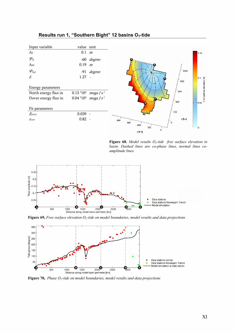
XI
Input variable value unit
A0 0.1 m
0ϕ -60 degree
A0d 0.19 m
d0ϕ -91 degree
fs 1.27 -
Energy parameters
North energy flux in 0.13 *103 mega J s-1
Dover energy flux in 0.04 *103 mega J s-1
Fit parameters
Eerror 0.039 -
rcorr 0.82 -
Figure 68. Model results O1-tide free surface elevation in
basin. Dashed lines are co-phase lines, normal lines co-
amplitude lines.
Figure 69, Free surface elevation O1-tide on model boundaries, model results and data projections
Figure 70, Phase O1-tide on model boundaries, model results and data projections
Results run 1, “Southern Bight” 12 basins O1-tide