on the structure of continua with ﬁnite length and gołąb’s...

version: September 29, 2017 (revised) † Nonlinear Analysis 153 (2017), 35-55DOI: 10.1016/j.na.2016.10.012

On the structure of continua with finite length

and Gołąb’s semicontinuity theorem

Giovanni Alberti and Martino Ottolini

Dedicated to Nicola Fusco on the occasion of his 60th birthday

Abstract. The main results in this note concern the characterization of the lengthof continua 1 (Theorems 2.5) and the parametrization of continua with finite length(Theorem 4.4). Using these results we give two independent and relatively elementaryproofs of Gołąb’s semicontinuity theorem.

Keywords: continua with finite length, Hausdorff measure, Gołąb’s semicontinuitytheorem.

MSC (2010): 28A75, 54F50, 26A45, 49J45, 49Q20.

1. Introduction

Let F be the class of all continua K contained in Rd, endowed with the Hausdorff

distance. A classical result due to S. Gołąb (see [8], Section 3, or [6], Theorem 3.18)states that the length, that is, the function K 7! H 1(K), is lower semicontinuouson F . Variants of this semicontinuity result, together with well-known compactnessproperties of F , play a key role in the proofs of several existence results in theCalculus of Variations, from optimal networks [9] to image segmentation [2] and quasi-static evolution of fractures [3]. In particular, Gołąb’s theorem has been extended togeneral metric spaces in [1], Theorem 4.4.17, and [9], Theorem 3.3.2

It should be noted that none of the proofs of Gołąb’s theorem mentioned above iscompletely elementary. On the other hand, the counterpart of this result for paths,namely that the length of a path γ : [0, 1] ! X is lower semicontinuous with respect tothe pointwise convergence of paths, is elementary and almost trivial. This sharp con-trast is due to the fact that the definitions of length of a path and of one-dimensionalHausdorff measure of a set are utterly different, even though they aim to describe(essentially) the same geometric quantity. More precisely, the length of a path, beingdefined as a supremum of finite sums which are clearly continuous, is naturally lowersemicontinuous, while the definition of Hausdorff measure is based on Caratheodory’sconstruction, and is designed to achieve σ-subadditivity, not semicontinuity.

In this note we point out a couple of relations/similarities between the one-dimensional Hausdorff measure of continua and the length of paths, which we then

† Compared to the published version, we have added two pictures, corrected the proof ofLemma 2.22 and a few small mistakes, and modified the definition of δ-partition in Subsection 2.7,in order to make the statement of Proposition 2.8 stronger (consequently, we have also modifiedLemma 2.18).

1 As usual, a continuum is a connected compact metric space (or subset of a metric space), andthe length of a set is its one-dimensional Hausdorff measure H

1.2 The proof in [1] is actually incomplete; the missing steps were given in [9].

2 G. Alberti, M. Ottolini

use to give two independent (and relatively elementary) proofs of Gołąb’s theorem.We think, however, that these results are interesting in their own right.

Firstly, in Theorem 2.5 we show that for every continuum X there holds

H1(X) = sup

⇢

X

i

diam(Ei)

}

,

where the supremum is taken over all finite families {Ei} of disjoint connected subsetsof X. (Note the resemblance with the definition of length of a path.)

Secondly, in Theorem 4.4 we show that every continuum X with finite lengthadmits some sort of canonical parametrization; more precisely, there exists a pathγ : I ! X with length equal 2H 1(X) which “goes through almost every point of Xtwice, once moving in a direction, and once moving in the opposite direction”, theprecise statement requires some technical definitions and is postponed to Section 4.

This paper is organized as follows: Sections 2 and 4 contain the two results men-tioned above (Theorems 2.5 and 4.4) and the corresponding proofs of Gołąb’s theo-rem. Section 3 contains a review of some basic facts about paths with finite length ina metric space which are used in Section 4, and can be skipped by the expert reader.This review is self-contained and limited in scope; a more detailed presentation ofthe theory of paths with finite length in metric spaces can be found in [1], Chapter 4,while continua with finite length have been studied in detail in [4] (see also [7]).

Since the results described in this paper are rather elementary (in particular Theo-rem 2.5), we strove to keep the exposition self-contained, and avoid in particular theuse of advanced results from Geometric Measure Theory. On the other hand, proofsare sometimes just sketched, with all steps clearly indicated but many details left tothe reader.

2. A characterization of length

The main results in this section are the characterizations of the length of setswith countably many connected components (and in particular of continua) given inTheorem 2.5 and Proposition 2.8. Using the former result we give our first proof ofGołąb’s theorem (Theorem 2.9).

2.1. Notation. Through this paper X is a metric space endowed with the distanced. Given x 2 X and E,E0 subsets of X we set:

B(x, r) closed ball with center x and radius r > 0;

diam(E) diameter of E, i.e., sup{d(x, x0) : x, x0 2 E};

dist(x,E) distance between x and E, i.e., inf{d(x, x0) : x0 2 E};

dist(E,E0) distance between E and E0, i.e., inf{d(x, x0) : x 2 E, x0 2 E0};3

dH(E,E0) Hausdorff distance between E and E0, i.e., the infimum of all r ≥ 0 s.t.dist(x,E0) r for every x 2 E and dist(x0, E) r for every x0 2 E0;

Lip(f) Lipschitz constant of a map f between metric spaces;

|E| = L 1(E), Lebesgue measure of a Borel set E contained in R.

2.2. Hausdorff measure. For every set E contained in X, the one-dimensionalHausdorff measure of E is defined by

H1(E) := sup

δ>0H

1δ (E) = lim

δ!0H

1δ (E) ,

3 Since the infimum of the empty set is +∞, dist(E,E0) = +∞ if either E or E0 are empty.

Continua with finite length 3

where, for every δ 2 (0,+1],

H1δ (E) := inf

⇢

X

i

diam(Ei)

}

,

the infimum being taken over all countable families {Ei} of subsets of X which coverE and satisfy diam(Ei) δ.

2.3. Remark. Among the many properties of H 1 we recall the following ones.

(i) H 1 is a σ-subadditive set function (that is, an outer measure on X) and isσ-additive on Borel sets. Moreover H 1 agrees with the (outer) Lebesgue measureL 1 when X = R.

(ii) Given a Lipschitz map f : X ! Y , for every set E contained in X there holdsH 1(f(E)) Lip(f)H 1(E).

(iii) If H 1δ (E) = 0 for some δ 2 (0,+1] then H 1(E) = 0.

2.4. The set function Lδ. For every δ 2 (0,+1] and every set E in X we define

Lδ(E) := sup

⇢

X

i

diam(Ei)

}

,

where the supremum is taken over all finite, disjoint families {Ei} of continua con-tained in E with diam(Ei) δ.

2.5. Theorem. Let E be a subset of X which is locally compact and has countablymany connected components.4 Then, for every δ 2 (0,+1],

H1(E) = Lδ(E) . (2.1)

2.6. Remark. (i) The assumption that E has countably many connected componentscannot be dropped. Indeed Lδ(E) = 0 for every totally disconnected set E, and thereare examples of such sets with H 1(E) > 0, even compact and contained in R.

(ii) Theorem 2.5, together with Lemma 2.11, implies the following weaker state-ment: for any set E as above, H 1(E) agrees with the supremum of

P

i diam(Ei) overall finite disjoint families {Ei} of connected subsets of E. Concerning this identity,it is not clear if the assumption that E is locally compact can be weakened or evenremoved. The role of compactness in our proof is briefly discussed in Remark 2.16.

Using Theorem 2.5 we can actually show that H 1(E) can be approximated byP

i diam(Ei) using any partition of E made of connected subsets Ei with sufficientlysmall diameters. For a precise statement we need the following definition.

2.7. δ-Partitions. Let E be a subset of X and let δ 2 (0,+1]. We say that acountable family {Ei} of subsets of E is a δ-partition of E if the sets Ei are Borel,connected, H 1-essentially disjoint (i.e., H 1(Ei \ Ej) = 0 for every i 6= j), cover allof E except a subset E0 with H 1(E0) 0, and satisfy diam(Ei) δ.

If E is locally compact, has finite length and countably many connected compo-nents, then Theorem 2.5 implies that there exist δ-partitions for every δ > 0.

4 A connected component of E is any element of the class of nonempty connected subsets of Ewhich is maximal with respect to inclusion; the connected components are closed in E, disjoint, andcover E (for more details see [5], Chapter 6).


2.8. Proposition. Let E be a subset of X. Then every δ-partition {Ei} of E satisfies

H1(E) ≥

X

i

H1(Ei) ≥

X

i

diam(Ei) . (2.2)

If in addition E is locally compact and has countably many connected components,then for every m < H 1(E) there exists δ0 > 0 such that every δ-partition {Ei} of Ewith δ δ0 satisfies

X

i

diam(Ei) ≥ m. (2.3)

Using Theorem 2.5 we can also prove the following version of Gołąb’s theorem.

2.9. Theorem. For every m = 1, 2, . . . , let Fm be the class of all nonempty compactsubsets of X with at most m connected components. Then the function K 7! H 1(K)is lower-semicontinuous on Fm endowed with the Hausdorff distance.

2.10. Remark. The statement of Gołąb’s theorem is often restricted to the casem = 1, and in the metric setting reads as follows (cf. [1], Theorem 4.4.17): let begiven a sequence of continua Kn, contained in a complete metric space X, whichconverge in the Hausdorff distance to some closed set K; then K is a continuum, andlim inf H 1(Kn) ≥ H 1(K). The assumption that X is complete is needed here toensure that the limit K is compact and connected, but not to prove the semicontinuityof length.

The rest of this section is devoted to the proofs of Theorems 2.5 and 2.9, and Propo-sition 2.8. We begin with the proof of Theorem 2.5; the key estimate is contained inLemma 2.17.

2.11. Lemma. Let E be a connected set in X. Then H 1(E) ≥ diam(E).

Proof. It suffices to prove that H 1(E) ≥ d(x0, x1) for every x0, x1 2 E. Let indeedf : X ! R be the function defined by f(x) := d(x, x0). Then

H1(E) ≥ |f(E)| = diam(f(E)) ≥ |f(x1)− f(x0)| = d(x1, x0) ,

where the first inequality follows from Remark 2.3(ii) (and Lip(f) = 1), while the firstequality follows from the fact that f(E) is an interval (because E is connected). ⇤

2.12. Lemma. For every set E in X and δ > 0 there holds H 1(E) ≥ Lδ(E).

Proof. Consider any family {Ei} as in the definition of Lδ(E): Lemma 2.11 yields

H1(E) ≥

X

i

H1(Ei) ≥

X

i

diam(Ei) ,

and we obtain H 1(E) ≥ Lδ(E) by taking the supremum over all {Ei}. ⇤

2.13. Lemma. Let E be a subset of X and let {Ei} be the family of all connectedcomponents of E. Then Lδ(E) =

P

i Lδ(Ei) for every δ > 0.5

The proof of this lemma is straightforward, and we omit it.

5 The sum at the right-hand side of this equality is defined as the supremum of all finite subsums,and is well defined even if the family {Ei} is uncountable.


2.14. Lemma. Let U be a nonempty compact set in X, and let F be a connected com-ponent of U . If F \@U = ? then F is also a connected component of X. Accordingly,if X is connected and F 6= X then F \ @U 6= ?.

Proof. Let F be the family of all sets A such that F ⇢ A ⇢ U and A is openand closed in U . Then F is closed by finite intersection, and F agrees with theintersection of all A 2 F (see [5], Theorem 6.1.23).

If F \ @U = ? then the intersection of the compact sets A \ @U with A 2 F isempty, which implies that A\@U is empty for at least one A 2 F .6 This means thatF is the intersection of all A 2 F such that A\ @U = ?. Note that these sets A areopen and closed in X, and then F is connected and agrees with the intersection ofa family of open and closed sets. This implies that F is a connected component ofX. ⇤

2.15. Corollary. Let E be a connected set in X, let B = B(x, r) be a ball withcenter x 2 E such that E \B is compact and E \B 6= ?, and let F be the connectedcomponent of E \B that contains x. Then H 1(B \ E) ≥ H 1(F ) ≥ r.

Proof. By applying Lemma 2.14 with E and E \B in place of X and U , we obtainthat F intersects @B. Then diam(F ) ≥ r, and Lemma 2.11 yields H 1(F ) ≥ r. ⇤

2.16. Remark. The compactness assumptions in Lemma 2.14 and Corollary 2.15 areboth necessary. Indeed it is possible to construct a bounded connected set E in R

2

and a ball B with center x 2 E such that E \B 6= ?, but the connected componentF of E \ B that contains x consists just of the point x; in particular F \ @B = ?,and H 1(F ) = 0.

2.17. Lemma. Let E be a set in X which is connected and locally compact. ThenH 1

δ (E) Lδ(E) for every δ > 0.

Proof. We can clearly assume that Lδ(E) is finite. We fix for the time being " > 0,and choose a finite disjoint family {Ei} of continua contained in E with diam(Ei) δsuch that

X

i

diam(Ei) ≥ Lδ(E)− " . (2.4)

Next we set E0 := E \(

[i Ei

)

. Since the union of all Ei is closed and E is locallycompact, for every x 2 E0 we can find a ball B(x, r) with radius r δ/10 such thatE \ B(x, r) is compact and contained in E0. Using Vitali’s covering lemma (cf. [1],Theorem 2.2.3), we can extract from this family of balls a subfamily of disjoint ballsBj = B(xj , rj) such that the balls B0

j := B(xj , 5rj) cover E0.

Then the balls B0j together with the sets Ei cover the set E, and since their diam-

eters do not exceed δ, the definition of H 1δ (E) yields

H1δ (E)

X

i

diam(Ei) +X

j

diam(B0j) Lδ(E) + 10

X

j

rj . (2.5)

On the other hand, by Corollary 2.15, for every j we can find a closed, connectedset Fj contained in Bj \ E with diameter at least rj . Since the balls Bj are disjointand contained in E0, we have that the sets Fj together with the sets Ei form a disjoint

6 The basic fact behind this assertion is that every family of compact sets with empty intersectionadmits a finite subfamily with empty intersection.


family of continua contained in E with diameters at most δ, and therefore, using thedefinition of Lδ(E) and (2.4),

Lδ(E) ≥X

i

diam(Ei) +X

j

diam(Fj) ≥ Lδ(E)− "+X

j

rj ,

which implies " ≥P

j rj . Hence (2.5) yields H 1δ (E) Lδ(E)+ 10 ", and the proof is

complete because " is arbitrary. ⇤

Proof of Theorem 2.5. By Lemma 2.12, it suffices to prove that

Lδ(E) ≥ H1(E) . (2.6)

We assume first that E is connected. In this case Lemma 2.17 and the definition ofLδ in Subsection 2.4 yield

Lδ(E) ≥ Lδ0(E) ≥ H1δ0 (E) for every 0 < δ0 δ,

and we obtain (2.6) by taking the limit as δ0 ! 0.If E is not connected, then (2.6) holds for every connected component of E, and

we obtain that it holds for E as well using Lemma 2.13, the subadditivity of H 1,and the fact that E has countably many connected components. ⇤

The next lemma is used in the proof of Proposition 2.8.

2.18. Lemma. Let F be a continuum in X, let {Ei} be a countable family of con-nected subsets of X, and let E0 be the union of all Ei. Then

H1(F \ E0) +

X

i

diam(Ei) ≥ diam(F ) .

Proof. Take x0, x1 2 F such that d(x0, x1) = diam(F ), and let f : X ! R be theLipschitz function given by f(x) := d(x, x0). Then

H1(F \ E0) +

X

i

diam(Ei) ≥ |f(F \ E0)|+X

i

diam(f(Ei))

= |f(F \ E0)|+X

i

|f(Ei)| ≥ |f(F )| ≥ diam(F ) ,

where the first inequality follows from the fact that Lip(f) = 1, for the equality weuse that each f(Ei) is an interval, for the second inequality we use that the sets f(Ei)together with f(F \E0) cover f(F ), and the last inequality follows from the fact thatf(F ) is an interval that contains f(x0) = 0 and f(x1) = d(x0, x1) = diam(F ). ⇤

Proof of Proposition 2.8. To prove (2.2) we use the definition of δ-partition andestimate H 1(Ei) ≥ diam(Ei) (see Lemma 2.11).

To prove the second part of the statement, we first choose δ1 > 0 such thatH 1(E) > m + δ1, and use Theorem 2.5 to find finitely many disjoint continua Fj

contained in E such thatX

j

diam(Fj) ≥ m+ δ1 . (2.7)

Then we take δ0 with 0 < δ0 δ1 such that dist(Fj , Fk) > δ0 for every j 6= k.Consider now any δ-partition {Ei} of E with δ δ0. Let E0 be the union of all i.

For every j, let Ij the the collection of all indices i such that Ei intersects Fj , and


let E0j be the union of all Ei with i 2 Ij . By the choice of δ0 the collections Ij are

pairwise disjoint, and therefore

H1(E \ E0) +

X

i

diam(Ei) ≥

≥X

j

H1(Fj \ E

0j) +

X

i2Ij

diam(Ei)

]

≥X

j

diam(Fj) ,

where the last inequality follows from Lemma 2.18. Since {Ei} is a δ-partition of Ewe obtain that

δ +X

i

diam(Ei) ≥X

j

diam(Fj) , (2.8)

and putting together (2.7), (2.8) and the fact that δ δ0 δ1 we obtain (2.3). ⇤

We now pass to the proof of Theorem 2.9.

2.19. δ-chains and δ-connected sets. Given δ > 0, a δ-chain in X is any finitesequence of points {xi : i = 0, . . . , n} contained in X such that d(xi−1, xi) δ forevery i > 0. We call x0 and xn endpoints of the δ-chain, and we say that the δ-chainconnects x0 and xn. The length of the δ-chain is

length({xi}) :=nX

i=1

d(xi−1, xi) .

Finally, we say that a set E in X is δ-connected if every couple of points x, x0 2 E isconnected by a δ-chain contained in E.

2.20. Lemma. If E is a connected set in X then it is δ-connected for every δ > 0.

Proof. Fix x 2 E and let Ax be the set of all points x0 2 E which are connected tox by a δ-chain contained in E. We must show that Ax = E.

One easily checks that:

• Ax is closed in E and contains x;

• if x0 2 Ax then B(x0, δ) \ E is contained in Ax; thus Ax is open in E.

Since Ax is nonempty, open and closed in E, and E is connected, we conclude thatAx = E, as desired. ⇤

2.21. Lemma. Let K be a compact set in X with at most m connected components,which contains a δ-connected subset K 0. Then

H1(K) ≥ diam(K 0)−mδ . (2.9)

Proof. We can assume that m is finite. We then take x0, x1 2 K 0 such that

` := d(x0, x1) ≥ diam(K 0)− δ , (2.10)

and let H := f(K) where f : X ! R is defined by f(x) := d(x, x0). It is easy tocheck that:

(a) Lip(f) = 1, and therefore H 1(K) ≥ |H| ≥ `−∣

∣(0, `) \H∣

∣;

(b) the sets f(K 0) and H contain 0 = f(x0) and ` = f(x1);

(c) H has at most m connected components because so does K;

(d) the set f(K 0) is δ-connected because K 0 is δ-connected and Lip(f) = 1.


Statements (b) and (c) imply that the open set (0, `) \ H has at most m − 1 con-nected components, while statements (b) and (d) imply that each of these connectedcomponents has length at most δ; in particular

∣

∣(0, `) \H∣

∣ (m− 1)δ . (2.11)

Using the estimate in (a), (2.10), and (2.11) we finally obtain (2.9). ⇤

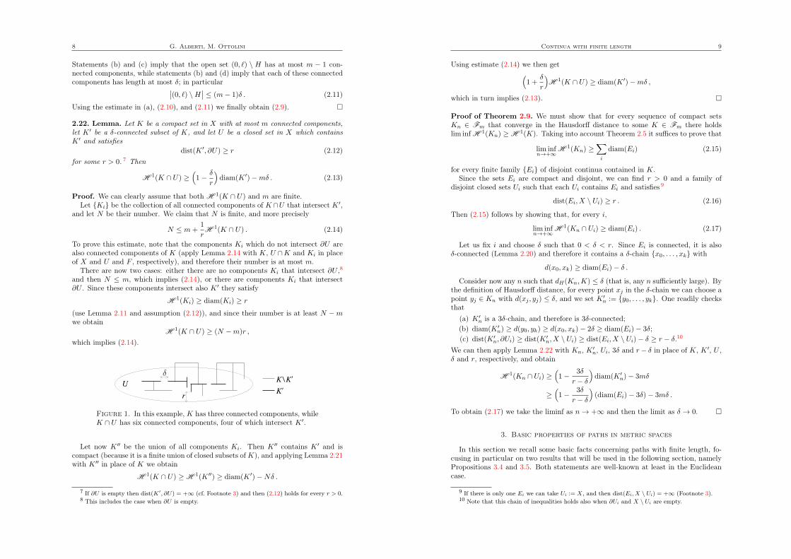
2.22. Lemma. Let K be a compact set in X with at most m connected components,let K 0 be a δ-connected subset of K, and let U be a closed set in X which containsK 0 and satisfies

dist(K 0, @U) ≥ r (2.12)

for some r > 0. 7 Then

H1(K \ U) ≥

⇣

1−δ

r

⌘

diam(K 0)−mδ . (2.13)

Proof. We can clearly assume that both H 1(K \ U) and m are finite.Let {Ki} be the collection of all connected components of K \U that intersect K 0,

and let N be their number. We claim that N is finite, and more precisely

N m+1

rH

1(K \ U) . (2.14)

To prove this estimate, note that the components Ki which do not intersect @U arealso connected components of K (apply Lemma 2.14 with K, U \K and Ki in placeof X and U and F , respectively), and therefore their number is at most m.

There are now two cases: either there are no components Ki that intersect @U ,8

and then N m, which implies (2.14), or there are components Ki that intersect@U . Since these components intersect also K 0 they satisfy

H1(Ki) ≥ diam(Ki) ≥ r

(use Lemma 2.11 and assumption (2.12)), and since their number is at least N −mwe obtain

H1(K \ U) ≥ (N −m)r ,

which implies (2.14).

U

δ

rK′

K \ K′

Figure 1. In this example, K has three connected components, whileK \ U has six connected components, four of which intersect K 0.

Let now K 00 be the union of all components Ki. Then K 00 contains K 0 and iscompact (because it is a finite union of closed subsets of K), and applying Lemma 2.21with K 00 in place of K we obtain

H1(K \ U) ≥ H

1(K 00) ≥ diam(K 0)−Nδ .

7 If ∂U is empty then dist(K0, ∂U) = +∞ (cf. Footnote 3) and then (2.12) holds for every r > 0.8 This includes the case when ∂U is empty.


Using estimate (2.14) we then get

⇣

1 +δ

r

⌘

H1(K \ U) ≥ diam(K 0)−mδ ,

which in turn implies (2.13). ⇤

Proof of Theorem 2.9. We must show that for every sequence of compact setsKn 2 Fm that converge in the Hausdorff distance to some K 2 Fm there holdslim inf H 1(Kn) ≥ H 1(K). Taking into account Theorem 2.5 it suffices to prove that

lim infn!+1

H1(Kn) ≥

X

i

diam(Ei) (2.15)

for every finite family {Ei} of disjoint continua contained in K.Since the sets Ei are compact and disjoint, we can find r > 0 and a family of

disjoint closed sets Ui such that each Ui contains Ei and satisfies 9

dist(Ei, X \ Ui) ≥ r . (2.16)

Then (2.15) follows by showing that, for every i,

lim infn!+1

H1(Kn \ Ui) ≥ diam(Ei) . (2.17)

Let us fix i and choose δ such that 0 < δ < r. Since Ei is connected, it is alsoδ-connected (Lemma 2.20) and therefore it contains a δ-chain {x0, . . . , xk} with

d(x0, xk) ≥ diam(Ei)− δ .

Consider now any n such that dH(Kn,K) δ (that is, any n sufficiently large). Bythe definition of Hausdorff distance, for every point xj in the δ-chain we can choose apoint yj 2 Kn with d(xj , yj) δ, and we set K 0

n := {y0, . . . , yk}. One readily checksthat

(a) K 0n is a 3δ-chain, and therefore is 3δ-connected;

(b) diam(K 0n) ≥ d(y0, yk) ≥ d(x0, xk)− 2δ ≥ diam(Ei)− 3δ;

(c) dist(K 0n, @Ui) ≥ dist(K 0

n, X \ Ui) ≥ dist(Ei, X \ Ui)− δ ≥ r − δ.10

We can then apply Lemma 2.22 with Kn, K 0n, Ui, 3δ and r− δ in place of K, K 0, U ,

δ and r, respectively, and obtain

H1(Kn \ Ui) ≥

⇣

1−3δ

r − δ

⌘

diam(K 0n)− 3mδ

≥⇣

1−3δ

r − δ

⌘

(diam(Ei)− 3δ)− 3mδ .

To obtain (2.17) we take the liminf as n ! +1 and then the limit as δ ! 0. ⇤

3. Basic properties of paths in metric spaces

In this section we recall some basic facts concerning paths with finite length, fo-cusing in particular on two results that will be used in the following section, namelyPropositions 3.4 and 3.5. Both statements are well-known at least in the Euclideancase.

9 If there is only one Ei we can take Ui := X, and then dist(Ei, X \ Ui) = +∞ (Footnote 3).10 Note that this chain of inequalities holds also when ∂Ui and X \ Ui are empty.


3.1. Paths. A path in X is a continuous map γ : I ! X where I = [a0, a1] is aclosed interval. Then x0 := γ(a0) and x1 := γ(a1) are called endpoints of γ, and wesay that γ connects x0 to x1. If x0 = x1 we say that γ is closed.

The multiplicity of γ at a point x 2 X is the number (possibly equal to +1)

m(γ, x) := #(γ−1(x)) .

The length of γ is

length(γ) = length(γ, I) := sup

⇢ nX

i=1

d(

γ(ti−1), γ(ti))

}

where the supremum is taken over all n = 1, 2, . . . and all increasing sequences{t0, . . . , tn} contained in I.11

The length of γ relative to a closed interval J contained in I, denoted bylength(γ, J), is the length of the restriction of γ to J . If γ has finite length it issometimes useful to consider the length measure associated to γ, namely the (unique)positive measure µγ on I which satisfies

µγ([t0, t1]) = length(γ, [t0, t1]) for every [t0, t1] ⇢ I.

We say that γ is a geodesic if it has finite length and minimizes the length amongall paths with the same endpoints.

We say that γ has constant speed if there exists a finite constant c such that

length(γ, [t0, t1]) = c(t1 − t0) for every [t0, t1] ⇢ I.

An (orientation preserving) reparametrization of γ is any path γ0 : I 0 ! X of theform

γ0 = γ ◦ ⌧

where ⌧ : I 0 ! I is an increasing homeomorphism.

3.2. Remark. Here are some elementary (and mostly well-known) facts.

(i) The length is lower semicontinuous with respect to the pointwise convergenceof paths. More precisely, given a sequence of paths γn : I ! X which convergepointwise to γ : I ! X, it is easy to check that

length(γ) lim infn!+1

length(γn) .

(ii) Every path γ : I ! X with finite length `, which is not constant on anysubinterval of I, admits a Lipschitz reparametrization γ0 : [0, 1] ! X with constantspeed `, namely γ0 := γ ◦ σ−1 where σ : I ! [0, 1] is the homeomorphism given by

σ(t) :=1

`length(γ, [a0, t]) for every t 2 I = [a0, a1].

(iii) If γ is constant on some subinterval of I then the function σ defined aboveis continuous, surjective, but not injective. However, we can still consider the left-inverse ⌧ defined by

⌧(s) := min{t : σ(t) = s} for every s 2 [0, 1],

and even though ⌧ is not continuous, one can check that γ0 := γ ◦ ⌧ is a continuouspath with constant speed `, and m(γ0, x) = m(γ, x) for all points x 2 X exceptcountably many.

11 The length of γ is sometimes called variation and denoted by Var(γ, I); paths with finite lengthare called rectifiable.


(iv) If γ is Lipschitz then length(γ, J) Lip(γ) |J | for every interval J contained inI, and more generally µγ(E) Lip(γ) |E| for every Borel set E contained in I. Thusthe length measure µγ is absolutely continuous with respect to the Lebesgue measureon I, and more precisely it can be written as µγ = ⇢L 1 with a density ⇢ : I ! R

such that 0 ⇢ Lip(γ) a.e.

(v) If γ has constant speed c then Lip(γ) = c, length(γ) = c |I| and µγ = cL 1.Conversely, it is easy to check that if Lip(γ) |I| length(γ) < +1 then γ hasconstant speed c = Lip(γ) = length(γ)/|I|.

3.3. Remark. The following result is worth mentioning, even though it will not beused in the following: if γ is Lipschitz and ⇢ is taken as in Remark 3.2(iv), then fora.e. t 2 I there holds

limh!0

d(

γ(t+ h), γ(t))

|h|= lim

h!0+

length(

γ, [t− h, t+ h])

2h= ⇢(t) . (3.1)

The second equality in (3.1) is a straightforward consequence of Lebesgue’s differen-tiation theorem, while the first one is not immediate and will not be proved here.The first limit in (3.1) is called metric derivative of γ (see [1], Definition 4.1.2 andTheorem 4.1.6).

We can now state the main results of this section.

3.4. Proposition. Let X be a continuum with H 1(X) < +1, and let x 6= x0 bepoints in X. Then x and x0 are connected by an injective geodesic γ : [0, 1] ! X withconstant speed and length ` H 1(X).

If X is a subset of Rn, this statement can be found for example in [6], Lemma 3.12.A slightly more general version of this statement (in the metric setting) can be foundin [1], Theorem 4.4.7. For the sake of completeness we give a proof below, whichfollows essentially the one in [6].

3.5. Proposition. Let γ : I ! X be a path with finite length. Then the multiplicitym(γ, ·) : X ! [0,+1] is a Borel function and

length(γ) =

Z

X

m(γ, x) dH 1(x) . (3.2)

In particular m(γ, x) is finite for H 1-a.e. x 2 X.

3.6. Remark. (i) Formula (3.2) can be viewed as the one-dimensional area formula inthe metric setting, in particular if coupled with the existence of the metric derivative,see Remark 3.3.

(ii) Formula (3.2) can easily re-written in local form: for every Borel functionf : X ! [0,+1] there holds

Z

I

f(γ(t)) dµγ(t) =

Z

X

f(x)m(γ, x) dH 1(x) . (3.3)

This means that the push-forward of the length measure µγ according to the mapγ agrees with the measure H 1 on X multiplied by the density m(γ, ·); in shortγ#(µγ) = m(γ, ·)H 1.

The rest of this section is devoted to the proofs of Propositions 3.4 and 3.5. Webegin with some preliminary lemmas.


3.7. Lemma. Take X,x, x0 as in Proposition 3.4. Then, for every δ > 0, x and x0

are connected by a δ-chain {xi : i = 0, . . . , n} (see Subsection 2.19) such that

length({xi}) 4H1(X) . (3.4)

Proof. We can assume δ < d(x, x0), otherwise it suffices to take the δ-chain consistingjust of the points x, x0 and use Lemma 2.11 to obtain (3.4).

By Lemma 2.20, x and x0 are connected a δ-chain {xi}, and possibly removingsome points from the chain, we can further assume that

d(xi, xj) > δ if |j − i| ≥ 2. (3.5)

Consider now the balls Bi := B(xi, δ/2) with i = 0, . . . , n, and note that H 1(Bi) ≥δ/2 by Corollary 2.15, while (3.5) implies that Bi and Bj do not intersect if |j−i| ≥ 2,which means that every point in X belongs to at most two balls in the family {Bi}.Using these facts and the estimate δ ≥ d(xi−1, xi) we obtain

2H1(X) ≥

nX

i=0

H1(Bi) ≥

nX

i=0

δ

2≥

1

2length({xi}) . ⇤

3.8. Lemma. For every path γ : I ! X there holds H 1(γ(I)) length(γ).

Proof. It suffices to show that H 1δ (γ(I)) length(γ) for every δ > 0 (cf. Subsec-

tion 2.2). Using the continuity of γ, we partition I into finitely many closed intervalsIi with disjoint interiors so that

diam(γ(Ii)) δ for every i.

Using the definition of H 1δ and the fact that diam(γ(Ii)) length(γ, Ii), we obtain

H1δ (γ(I))

X

i

diam(γ(Ii)) X

i

length(γ, Ii) = length(γ) . ⇤

3.9. Lemma. If γ : I ! X is an injective path then length(γ) = H 1(γ(I)).

Proof. By Lemma 3.8 and the definition of length it suffices to show that for everyincreasing sequence {t0, . . . , tn} in I there holds

nX

i=1

d(

γ(ti−1), γ(ti))

H1(γ(I)) .

Since the sets Ei := γ([ti−1, ti]) are connected, then diam(Ei) H 1(Ei) (Lemma 2.11),and since γ is injective, the intersection Ei \Ej contains at most one point for everyi 6= j, and in particular is H 1-null. Hence

nX

i=1

d(

γ(ti−1), γ(ti))

nX

i=1

diam(Ei) nX

i=1

H1(Ei) H

1(γ(I)) . ⇤

Proof of Proposition 3.4. The idea is simple: for every δ > 0 we take the (almost)shortest δ-chain {xδi } that connects x and x0, and consider the set Γδ of all couples(tδi , x

δi ) 2 [0, 1]⇥X with suitably chosen times tδi 2 [0, 1]. Passing to a subsequence,

we can assume that the compact sets Γδ converge in the Hausdorff distance to somelimit set Γ as δ ! 0; we then show that Γ is the graph of a path γ : [0, 1] ! X withthe desired properties.

We set I := [0, 1] and L := H 1(X). The proof is divided in several steps.


Step 1: construction of the δ-chain {xδi }. Fix δ > 0, and let Fδ be the class ofall δ-chains with initial point x and final point x0, and let Lδ be the infimum of thelength over all δ-chains in Fδ. By Lemma 3.7 we know that Fδ is not empty andLδ 4L.

We then choose a δ-chain {xδi : i = 0, . . . , nδ} in Fδ whose length `δ satisfies

Lδ `δ Lδ + δ 4L+ δ . (3.6)

Step 2: construction of the set Γδ. Fix δ > 0 and let {xδi : i = 0, . . . , nδ} be the δ-chain chosen in Step 1. We can clearly assume that the points xδi are all different, andfind an increasing sequence of numbers tδi with i = 0, . . . , nδ such that the first oneis 0, the last one is 1, and the differences tδi − tδi−1 are proportional to the distancesd(xδi−1, x

δi ). This means that

d(xδi−1, xδi )

tδi − tδi−1

= `δ (3.7)

for every i = 1, . . . , nδ, and in particular we have that

tδi − tδi−1 =d(xδi−1, x

δi )

`δ

δ

`δ

δ

d(x, x0). (3.8)

Finally, we set

Γδ :={

(tδi , xδi ) : i = 0, . . . , nδ

.

Step 3: construction of the set Γ. The sets Γδ defined in Step 2 are contained in thecompact metric space [0, 1]⇥X, and by Blaschke’s selection theorem (see for example[1], Theorem 4.4.15) we have that, possibly passing to a subsequence, they convergein the Hausdorff distance as δ ! 0 to some compact set Γ contained in [0, 1]⇥X.

Step 4: Γ is the graph of a Lipschitz path γ : I ! X. Formula (3.7) implies thateach Γδ is the graph of a map γδ from a subset of I to X with Lipschitz constant `δ.This immediately implies that Γ is the graph of a Lipschitz map γ from a subset ofI to X with Lip(γ) ` where (recall (3.6))

` := lim infδ!0

`δ = lim infδ!0

Lδ 4L . (3.9)

Moreover the projection of Γδ on I is the set Iδ := {tδi }, and taking into accountestimate (3.8) and the fact that Iδ contains 0 and 1, we get that Iδ converges to Iin the Hausdorff distance as δ ! 0. This implies that the projection of Γ on I is Iitself, which means that the domain of γ is I.

Step 5: γ connects x and x0. Since xδ0 = x and xδnδ= x0 for every δ > 0, each

Γδ contains the points (0, x) and (1, x0), and therefore so does Γ, which means thatγ(0) = x and γ(1) = x0.

Step 6: ` length(γ). For every δ > 0 we can extract from the image of γ aδ-chain that connects x and x0 and has length at most length(γ). This implies that`δ length(γ) (cf. Step 1), and using (3.9) we obtain the claim.

Step 7: γ has constant speed, and length(γ) = `. By Step 4 and Step 6 we havethat Lip(γ) ` length(γ). Then the claim follows from Remark 3.2(v).

Step 8: γ is a geodesic. Let γ0 be any path connecting x and x0. Arguing as inStep 6 we obtain ` length(γ0), which implies length(γ) length(γ0) by Step 7.


Step 9: γ is a injective. Assume by contradiction that there exists t0 2 I and s > 0such that γ(t0) = γ(t0 + s). Then the path γ0 : [0, 1− s] ! X defined by

γ0(t) :=

(

γ(t) if 0 t t0,

γ(t+ s) if t0 < t 1− s.

is well-defined, connects x and x0, and has length `(1 − s), which is strictly smallerthan the length of γ, contrary to the fact that γ is a geodesic.

Step 10: length(γ) H 1(X). Apply Lemma 3.9. ⇤

We pass now to the proof of Proposition 3.5.

3.10. Piecewise regular paths. Let I be a closed interval. We say that a finitefamily {Ii} is a partition of I if the Ii are closed intervals contained in I, have pairwisedisjoint interiors, and cover I, and we say that a path γ : I ! X is piecewise regularon the partition {Ii} if it is either constant or injective on each Ii.

3.11. Lemma. Let γ : I ! X be a path with finite length, and let {Ii} be a partitionof I. Then there exists a path γ0 : I ! X such that:

(i) γ0 is piecewise regular on the partition {Ii};

(ii) γ0 agrees with γ at the endpoints of each Ii and γ0(Ii) ⇢ γ(Ii);

(iii) length(γ0, Ii) = H 1(γ0(Ii)) H 1(γ(Ii)) length(γ, Ii) for every i.

Proof. We define γ0 on each interval Ii = [ai, a0i] as follows:

• if γ(ai) = γ(a0i) we let γ0 be the constant path γ(ai);

• if γ(ai) 6= γ(a0i), we let γ0 be any injective path from Ii to X 0 := γ(Ii) whichconnects γ(ai) to γ(a0i) (such path exists because X 0 has finite length, cf. Propo-sition 3.4).

The path γ0 satisfies statements (i) and (ii) by construction, while (iii) follows fromLemmas 3.8 and 3.9. ⇤

Proof of Proposition 3.5. The proof is divided in three cases.

Case 1: γ is injective. In this case the multiplicity m(γ, ·) is the characteristicfunction of the compact set γ(I), and therefore is Borel, while identity (3.2) followsfrom Lemma 3.9.

Case 2: γ is piecewise regular. We easily reduce to the previous case.

The general case. We choose a sequence of piecewise regular paths γn : I ! Xthat approximate γ in the following sense:

(a) γn converge to γ uniformly;

(b) length(γn) length(γ) for every n;

(c) m(γn, x) m(γ, x) for every x 2 X and every n;

(d) m(γn, x) ! m(γ, x) as n ! +1 for every x 2 X.

More precisely, we construct γn as follows: for every n we choose a partition {Ini } ofI so that

maxi

diam(Ini ) ! 0 as n ! +1. (3.10)

and then take γn according to Lemma 3.11. Then statements (a), (b), (c) and (d)can be readily derived from (3.10) and statements (ii) and (iii) in Lemma 3.11.


We can now prove that the multiplicity m(γ, ·) is Borel and (3.2) holds. The firstpart of this claim follows by the fact that m(γ, ·) agrees with the pointwise limit ofthe multiplicities m(γn, ·) (statement (d)), which are Borel measurable because thepaths γn fall into Case 2. To prove (3.2), note that statements (a) and (b) and thesemicontinuity of length imply that

(e) length(γn) ! length(γ) as n ! +1,

while statements (c) and (d) and Fatou’s lemma yield

(f)R

Xm(γn, ·) dH

1 !R

Xm(γ, ·) dH 1 as n ! +1.

We already know that (3.2) holds for each γn, and using statements (e) and (f) wecan pass to the limit (as n ! +1) and obtain that (3.2) holds for γ as well. ⇤

4. Parametrizations of continua with finite length

In this section we address the following question: can we parametrize a continuumX by a single path γ : I ! X, and if yes, what can we require about γ?

First of all, note that in general a continuum cannot be parametrized by a one-to-one path, and not even by a path with multiplicity equal to 1 at almost every point(take for example any network with a triple junction).12 On the other hand, it is easyto see that every network can be parametrized by a closed path that goes throughevery arc in the network twice, once in a direction and once in the opposite direction.

In Theorem 4.4 we show that something similar holds for every continuum X withfinite length, and more precisely there exists a closed path that goes through almostevery point of X twice, once in a direction and once in the opposite direction.

Before stating the result, we must give a precise formulation of the requirementin italic. If X is a network made of regular arcs of class C1 in R

n, we simply askthat γ has multiplicity equal to 2 and degree equal to 0 at every point of X exceptjunctions. The problem in extending this condition to general continua is that theusual definition of degree cannot be easily adapted to the metric setting. To getaround this issue, in Subsection 4.1 we introduce a suitable weaker notion of pathwith degree zero.

Unless further specification is made, in the following X is a metric space.

4.1. Paths with degree zero. Given a Lipschitz path γ : I ! X, a locally boundedBorel function f : X ! R, and a Lipschitz function g : X ! R, we introduce thenotation

Z

γ

f dg :=

Z

I

(f ◦ γ)d

dt(g ◦ γ) dt . (4.1)

Note that g ◦ γ is Lipschitz, and therefore the derivative in the integral at the right-hand side is well-defined at almost every t 2 I and bounded in t, and the integralitself is well-defined.

We say that γ has degree zero (at almost every point of its image) ifZ

γ

f dg = 0 for every f, g : X ! R Lipschitz. (4.2)

12 By network we mean here a connected union of finitely many arcs (that is, images of injectiveLipschitz paths) which intersect at most at the endpoints; a point which agrees with n endpoints,n ≥ 3, is called an n-junction.


4.2. Remark. (i) A simple approximation argument shows that if γ has degree zerothen

R

γf dg = 0 for every Lipschitz function g : X ! R and every bounded Borel

function f : X ! R.

(ii) If X is a finite union of oriented regular arcs in Rn, or more generally an

oriented 1-rectifiable set, and γ : I ! X is a Lipschitz path, then for H 1-almostevery x 2 X one can define the degree of γ at x, denoted by deg(γ, x). Moreover forevery f, g : X ! R there holds

Z

γ

f dg :=

Z

X

f(x)@g

@⌧(x) deg(γ, x) dH 1(x) , (4.3)

where @g/@⌧ is the tangential derivative of g. Using this formula it is easy to checkthat (4.2) holds if and only if deg(γ, x) = 0 for H 1-a.e. x 2 X. This justifies the useof the expression “path with degree zero” in Subsection 4.1.

(iii) Formula (4.2) can be reinterpreted in the framework of metric currents bysaying that the push-forward according to γ of the canonical 1-current associated tothe (oriented) interval I is trivial.

4.3. Proposition. Let γ : I ! X be a Lipschitz path, and let f, g : X ! R beLipschitz functions. Then the following statements hold.

(i) [Invariance under reparametrization] Let ⌧ : I 0 ! I be an increasing homeo-morphism such that γ ◦ ⌧ is Lipschitz. Then

Z

γ

f dg =

Z

γ◦τf dg . (4.4)

In particular, γ has degree zero if and only if γ ◦ ⌧ has degree zero.

(ii) [Stability] Given a sequence of paths γn : I ! X which are uniformly Lipschitzand converge uniformly to γ, then

Z

γn

f dg !

Z

γ

f dg as n ! +1.

In particular, if each γn has degree zero, then γ has degree zero.

(iii) [Parity] If γ has degree zero then the multiplicity m(γ, x) is finite and even forH 1-a.e. x 2 X.

We can now state the main result of this section.

4.4. Theorem. Let X be a continuum with finite length. Then there exists a pathγ : [0, 1] ! X with the following properties:

(i) γ is closed, Lipschitz, surjective, and has degree zero;

(ii) m(γ, x) = 2 for H 1-a.e. x 2 X, and length(γ) = 2H 1(X);

(iii) γ has constant speed, equal to 2H 1(X).

4.5. Remark. (i) The existence of a Lipschitz surjective path γ : [0, 1] ! X withLip(γ) 2H 1(X) was first proved in [10]. Here we simply point out that γ can betaken of degree zero.

(ii) An immediate corollary of this result is that every continuum X with finitelength is a rectifiable set of dimension 1.

(iii) If X is contained in Rn, then one can apply Rademacher’s differentiability

theorem to the parametrization γ and prove with little effort that X admits a tangentline in the classical sense at H 1-a.e. point.


The rest of this section is devoted to the proofs of Proposition 4.3 and Theorem 4.4.At the end of the section we give another proof of Gołąb’s theorem based on the latter.

4.6. Additional notation. Let be given a Lipschitz path γ : I ! X and a Lipschitzfunction g : X ! R. We write h := g ◦ γ, and denote by N the set of all s 2 R suchthat one of the following properties fails:

(a) the set h−1(s) is finite;

(b) the derivative h exists and is not 0 at every t 2 h−1(s).

Thus for every s 2 R \N and every x 2 g−1(s), the following sum is well-defined andfinite:

p(x) :=X

t2γ−1(x)

sgn(

h(t))

, (4.5)

where, as usual, sgn(x) := 1 if x > 0, sgn(x) := −1 if x < 0, and sgn(0) = 0.

4.7. Lemma. Take γ, g, h, N and p as in Subsection 4.6. Then |N | = 0 and forevery Lipschitz function f : X ! R there holds

Z

γ

f dg =

Z

R\N

X

x2g−1(s)

f(x) p(x)

]

ds . (4.6)

Proof. To prove that |N | = 0 we write

N = N0 [ h(E0) [ h(E1) ,

where N0 is the set of all s 2 R such that h−1(s) is infinite, E0 is the set of all t 2 Iwhere the derivative of h exists and is 0, E1 is the set of all t 2 I where the derivativeof h does not exists.

We observe now that |N0| = 0 and |h(E0)| = 0 by the one-dimensional area formulaapplied to the Lipschitz function h : I ! R,13 while |E1| = 0 by Rademacher’stheorem and then |h(E1)| = 0 because h is Lipschitz. We conclude that |N | = 0.

Let us prove (4.6). Using (4.1), the area formula, and that |N | = 0, we getZ

γ

f dg =

Z

I

(f ◦ γ) h dt =

Z

I

(f ◦ γ) sgn(h) |h| dt

=

Z

R\N

X

t2h−1(s)

f(γ(t)) sgn(h(t))

]

ds ,

and we obtain (4.6) by suitably rewriting the sum within square brackets. ⇤

Proof of Proposition 4.3(i). Given g and γ, we take h, N and p as in Subsec-tion 4.6, and let h0 N 0 and p0 be the analogous quantities where γ is replaced by γ ◦⌧ .Thanks to Lemma 4.7, identity (4.4) can be proved by showing that p(x) = p0(x) forevery x such that g(x) /2 \(N [N 0).

Taking into account (4.5) and the fact that h0 = h ◦ ⌧ , the identity p(x) = p0(x)reduces to the following elementary statement: given t 2 I such that the derivative of

13 The one-dimensional area formula we use reads as follows: if h : I → R is Lipschitz andf : I → R is either positive or in L1(I) then

Z

I

f |h| dt =

Z

R

X

t2h−1(s)

f(t)

]

ds .

In particularR

I|h| dt =

R

Rm(h, s) ds where m(h, s) is the multiplicity of h at s, which implies that

m(h, s) is finite for a.e. s ∈ R.


h at t exists and is nonzero, and the derivative of h0 = h ◦ ⌧ at t0 := ⌧−1(t) exists andis nonzero, then these derivatives have the same sign (recall that ⌧ is increasing). ⇤

Proof of Proposition 4.3(ii). In view of (4.1) it suffices to show thatZ

I

(f ◦ γn)d

dt(g ◦ γn) dt !

Z

I

(f ◦ γ)d

dt(g ◦ γ) dt as n ! +1.

This is an immediate consequence of the fact that the functions f ◦ γn converge tof ◦γ uniformly, and therefore strongly in L1(I), while the derivatives of the functionsg ◦ γn converge to the derivative of g ◦ γ in the weak* topology of L1(I). ⇤

The next lemmas are used in the proof of Proposition 4.3(iii).

4.8. Lemma. Let γ : I ! X be a path with finite length, and let µγ be the corre-sponding length measure (Subsection 3.1). Then for µγ-a.e. t 2 I there holds

⇢(t) := lim infr!0

diam(

γ(B(t, r)))

r> 0 . (4.7)

This lemma would be an immediate consequence of formula (3.1), which howeverwe did not prove. The proof below is self-contained.

Proof. Let E := {t 2 I : ⇢(t) = 0}. We must prove that µγ(E) = 0.Let " > 0 be fixed for the time being. For every t 2 E we can find rt > 0 such that

the ball (i.e., centered interval) B(t, rt) is contained in I and

diam(

γ(B(t, rt)))

"rt .

Consider now the family F of all balls B(t, rt/5) with t 2 E. Using Vitali’s coveringlemma (see for example [1], Theorem 2.2.3), we can extract from F a subfamily ofdisjoint balls Bj = B(tj , rj/5) such that the balls B0

j := B(tj , rj) cover E. Thus the

sets γ(B0j) cover γ(E) and can be used to estimate H 1

1(E) (see Subsection 2.2):

H11(γ(E))

X

j

diam(γ(B0j))

"X

j

rj =5"

2

X

j

|Bj | 5"

2|I|

(for the last inequality we used that the balls Bj are disjoint and contained in I).Since " is arbitrary, we obtain that H 1

1(γ(E)) = 0 and therefore H 1(γ(E)) = 0(cf. Remark 2.3(iii)). Using formula (3.3) we finally get

µγ(E) =

Z

γ(E)m(γ, x) dH 1(x) = 0 . ⇤

4.9. Lemma. Let γ : I ! X be a path with finite length, and let E be a Borel subsetof γ(I) with H 1(E) > 0. Then there exists a Lipschitz function g : X ! R such that|g(E)| > 0.

Proof. We can assume that γ has constant speed 1 (Remark 3.2(iii)), which impliesthat γ has Lipschitz constant 1 and the length measure µγ agrees with the Lebesguemeasure on I.

We set F := γ−1(E) and F 0 := I \ F . Since E = γ(F ) is not H 1-negligible, Fmust have positive Lebesgue measure, and using Lemma 4.8 and Lebesgue’s density


theorem we can find a point t 2 F where (4.7) holds and F has density 1, andaccordingly F 0 has density 0.

We define g : X ! R by g(x) := d(x, γ(t)), and set h := g ◦ γ. By (4.7) thereexists δ > 0 such that diam(γ(B(t, r))) ≥ 2δr for every ball B(t, r) contained in I.This implies that

supt02B(t,r)

h(t0) = supt02B(t,r)

d(γ(t0), γ(t)) ≥ δr .

Thus the interval h(B(t, r)) contains [0, δr] and then∣

∣h(B(t, r))∣

∣ ≥ δr . (4.8)

On the other hand, the fact that h is Lipschitz and F 0 has density 0 at t implies∣

∣h(F 0 \B(t, r))∣

∣ = o(r) . (4.9)

Finally, the inclusion

g(E) = h(F ) ⊃ h(B(t, r)) \ h(F 0 \B(t, r)) ,

together with estimates (4.8) and (4.9), yields

|g(E)| ≥ δr − o(r) ,

and we conclude by observing that δr − o(r) > 0 for r small enough. ⇤

Proof of Proposition 4.3(iii). We already know that m(γ, x) is finite for H 1-a.e. x 2 X (Proposition 3.5). Let then E be the set of all x 2 X such that m(γ, x) isfinite and odd, and assume by contradiction that H 1(E) > 0.

By Lemma 4.9 there exists a Lipschitz function g : X ! R such that |g(E)| > 0.Then we take N and p as in Subsection 4.6, and let f : X ! R be given by

f(x) :=

(

sgn(p(x)) if x 2 E \ g−1(N),

0 otherwise.

For this choice of g and f , the sum between square brackets in formula (4.6) is apositive odd integer for every s 2 g(E) \ N and is 0 otherwise, and therefore (4.6)yields

Z

γ

f dg ≥ |g(E) \N | = |g(E)| > 0 .

This contradicts the assumption that γ has degree zero (cf. Remark 4.2(i)). ⇤

The following construction is used in the proof of Theorem 4.4.

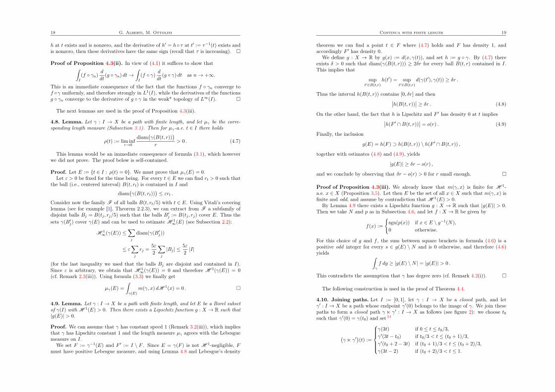
4.10. Joining paths. Let I := [0, 1], let γ : I ! X be a closed path, and letγ0 : I ! X be a path whose endpoint γ0(0) belongs to the image of γ. We join thesepaths to form a closed path γ n γ0 : I ! X as follows (see figure 2): we choose t0such that γ0(0) = γ(t0) and set 14

(

γ n γ0)

(t) :=

8

>

>

>

<

>

>

>

:

γ(3t) if 0 t t0/3,

γ0(3t− t0) if t0/3 < t (t0 + 1)/3,

γ0(t0 + 2− 3t) if (t0 + 1)/3 < t (t0 + 2)/3,

γ(3t− 2) if (t0 + 2)/3 < t 1.


(a) (b) (c)

γ(I)

x0

γ′(I)

x2

x1

γ� γ′(I)

x2

x1

x0

Figure 2. Example of joined paths: γ, γ0 and γnγ0 are described in(a), (b), (c), respectively (the arrows show how each path goes throughits own image); x0 agrees with both endpoints of γ and γn γ0, x1 andx2 are the endpoints of γ0, and x1 = γ0(0) = γ(t0).

The next lemma collects some straightforward properties of γnγ0 that will be usedlater. We omit the proof.

4.11. Lemma. Take γ, γ0 and γnγ0 as in Subsection 4.10. The following statementshold:

(i) if γ and γ0 are Lipschitz, then γ n γ0 is Lipschitz;

(ii) length(γ n γ0) = length(γ) + 2 length(γ0);

(iii) if γ and γ0 have bounded multiplicities, so does γ n γ0;

(iv) if the path γ has multiplicity 2 at all points in its image except finitely many,γ0 has multiplicity 1 at all points in its image except finitely many, and the setγ(I) \ γ0(I) is finite, then γ n γ0 has multiplicity 2 at all points in its imageexcept finitely many;

(v) for every f : X ! R bounded and Borel, and every g : X ! R Lipschitz thereholds

Z

γnγ0

f dg =

Z

γ

f dg ;

(vi) if γ has degree zero (cf. Subsection 4.1) then γ n γ0 has degree zero.

Proof of Theorem 4.4. Let I := [0, 1]. We obtain the path γ : I ! X with therequired properties as limit of the closed paths γn : I ! X constructed by theinductive procedure described in the next two steps.

Step 1: construction of γ1. We choose x00 2 X and take x0 2 X which maximizesthe distance from x00. By Proposition 3.4, there exists an injective Lipschitz pathγ00 : I ! X that connects x00 to x0. We then set

γ1(t) :=

(

γ00(2t) if 0 t 1/2,

γ00(2− 2t) if 1/2 < t 1.

Note that that γ1 is closed, has degree 0, and its multiplicity is 2 at all points of γ1(I)except γ1(1/2), where it is 1. Clearly length(γ1) = 2 length(γ00).

14 The notation γnγ0 is not quite appropriate, because this path does not depend only on γ andγ0, but also on the choice of t0.


Step 2: construction of γn+1, given γn. We assume that γn(I) is a proper subsetof X.15 Then we take a point xn 2 X which maximizes the distance from γn(I), andan injective Lipschitz path γ0n : I ! X that connects xn to some point x0n 2 γn(I).

By “cutting off a piece of γ0n” we can assume that this path intersects γn(I) onlyat the endpoint x0n. We can also assume that x0n = γ0n(0). Then we set

γn+1 := γn n γ0n .

Step 3: properties of γn. Using Lemma 4.11, one easily proves that each γn isclosed and Lipschitz, has degree zero, and satisfies

`n := length(γn) = 2n−1X

m=0

length(γ0m) . (4.10)

Moreover the multiplicity of γn is bounded and equal to 2 for all points in γn(I)except finitely many. This last property, together with formula (3.2), yields

`n := length(γn) 2H1(X) . (4.11)

Step 4: reparametrization of γn. Since the multiplicity of γn is bounded, γn is notconstant on any subinterval of I, and therefore it admits a reparametrization withconstant speed equal to `n (Remark 3.2(ii)). In the rest of the proof we replace γnby this reparametrization, which still satisfies all the properties stated in Step 3.

Step 5: construction of γ. The paths γn : I ! X are closed and uniformlyLipschitz, and more precisely Lip(γn) = `n 2H 1(X). Therefore, possibly passingto a subsequence, the paths γn converge uniformly to a path γ : I ! X which isclosed and Lipschitz, and satisfies Lip(γ) 2H 1(X).

Step 6: γ is surjective. Equations (4.10) and (4.11) imply that the sum of thelengths of all paths γ0n is finite, and then

length(γ0n) ! 0 as n ! +1.

Now, recalling the choice of xn and the fact that γ0n connects xn to γn(I) (cf. Step 2)we obtain that

dn := supx2X

dist(x, γn(I)) = dist(xn, γn(I)) length(γ0n) ,

and therefore dn tends to 0 as n ! +1, which means that the union of all γn(I) isdense in X.

Now, γm(I) contains γn(I) for every m ≥ n, and then γ(I) contains γn(I) for everyn. Hence γ(I) contains a dense subset of X, and since it is closed, it must agree withX.

Step 7: completion of the proof. Since the paths γn have degree zero, so doesγ (Proposition 4.3(ii)), and the proof of statement (i) is complete. This fact, thesurjectivity of γ, and Proposition 4.3(iii) imply that

m(γ, x) ≥ 2 for H1-a.e. x 2 X. (4.12)

On the other hand, estimate (4.11) and the semicontinuity of the length (Re-mark 3.2(i)) imply

length(γ) 2H1(X) . (4.13)

15 This inductive procedure stops if γn is surjective; when this happens, we simply reparametrizeγn so that it has constant speed, and set γ := γn. In this case it is quite easy to verify that γ hasthe required properties (we omit the details).


Now, equations (4.12) and (4.13), together with (3.2), imply that equality must holdboth in (4.12) and in (4.13), and statement (ii) is proved.

To prove statement (iii), note that Lip(γ) 2H 1(X) = length(γ) (cf. Step 5),and then γ must have constant speed (cf. Remark 3.2(v)). ⇤

We conclude this section by another proof of Gołąb’s theorem.

Second proof of Theorem 2.9 for m = 1. We must show that for every sequenceof continua Kn contained in X which converge in the Hausdorff distance to somecontinuum K, there holds lim inf H 1(Kn) ≥ H 1(K).

We can clearly assume that the lengths H 1(Kn) are uniformly bounded. Forevery n, we apply Theorem 4.4 to the continuum Kn and find a path γn : I ! Xwith I := [0, 1] such that γn(I) = Kn, γn has constant speed and degree zero, andlength(γn) = Lip(γn) = 2H 1(Kn).

Note that the paths γn are uniformly Lipschitz, and therefore, possibly passing to asubsequence, they converge uniformly to some path γ : I ! X, and clearly γ(I) = K.

Moreover Proposition 4.3(ii) implies that γ has degree zero, and Proposition 4.3(iii)implies that m(γ, x) ≥ 2 for H 1-a.e. x 2 K. Then formula (3.2) implies thatlength(γ) ≥ 2H 1(K).

We can now conclude, using the semicontinuity of length (cf. Remark 3.2(i)):

lim infn!+1

H1(Kn) =

1

2lim infn!+1

length(γn) ≥1

2length(γ) ≥ H

1(K) . ⇤

Acknowledgements

We thank Alexey Tuzhilin for pointing out a mistake in the proof of Lemma 2.22and for several valuable comments.

The research of the first author has been partially supported by the Universityof Pisa through the 2015 PRA Grant “Variational methods for geometric problems”,and by the European Research Council (ERC) through the Advanced Grant “Localstructure of sets, measures and currents”.

References

[1] Ambrosio, Luigi; Tilli, Paolo. Selected topics on analysis in metric spaces. Oxford LectureSeries in Mathematics and its Applications, vol. 25. Oxford University Press, Oxford, 2004.

[2] Dal Maso, Gianni; Morel, Jean-Michel; Solimini, Sergio. A variational method inimage segmentation: existence and approximation results. Acta Math., 168 (1992), 89–151.

[3] Dal Maso, Gianni; Toader, Rodica. A model for the quasi-static growth of brittle fractures:existence and approximation results. Arch. Ration. Mech. Anal., 162 (2002), no. 2, 101–135.

[4] Eilenberg, Samuel; Harrold, Orville G., Jr. Continua of finite linear measure. I. Amer.J. Math., 65 (1943), no. 1, 137–146.

[5] Engelking, Ryszard. General topology. Revised and completed edition. Sigma Series in PureMathematics, vol. 6. Heldermann Verlag, Berlin 1989.

[6] Falconer, Kenneth J. The geometry of fractal sets. Cambridge Tracts in Mathematics,vol. 85. Cambridge University Press, Cambridge, 1986.

[7] Fremlin, David H. Spaces of finite length. Proc. London Math. Soc. (3), 64 (1992), no. 3,449–486.

[8] Gołąb, Stanisław. Sur quelques points de la théorie de la longueur (On some points of thetheory of the length). Ann. Soc. Polon. Math., 7 (1929), 227–241.


[9] Paolini, Emanuele; Stepanov, Eugene. Existence and regularity results for the Steinerproblem. Calc. Var. Partial Differential Equations, 46 (2013), 837–860.

[10] Ważewski, Tadeusz. Kontinua prostowalne w związku z funkcjami i odwzorowaniami abso-lutnie ciągłemi (Rectifiable continua in connection with absolutely continuous functions andmappings). Dodatek do Rocznika Polskiego Towarzystwa Matematycznego (Supplement to theAnnals of the Polish Mathematical Society), (1927), 9–49.

G.A.Dipartimento di Matematica, Università di Pisalargo Pontecorvo 5, 56127 Pisa, Italye-mail: [email protected]

M.O.Scuola Normale Superiorepiazza dei Cavalieri 7, 56126 Pisa, Italye-mail: [email protected]

on the structure of continua with ﬁnite length and gołąb’s...

Documents