Louisiana State University Louisiana State University

LSU Digital Commons LSU Digital Commons

LSU Master's Theses Graduate School

October 2020

On the Stress Concentration at Sharp V-Notches Under Tension On the Stress Concentration at Sharp V-Notches Under Tension

Trent Mattieu Andrus Louisiana State University and Agricultural and Mechanical College

Follow this and additional works at: https://digitalcommons.lsu.edu/gradschool_theses

Part of the Applied Mechanics Commons

Recommended Citation Recommended Citation Andrus, Trent Mattieu, "On the Stress Concentration at Sharp V-Notches Under Tension" (2020). LSU Master's Theses. 5218. https://digitalcommons.lsu.edu/gradschool_theses/5218

This Thesis is brought to you for free and open access by the Graduate School at LSU Digital Commons. It has been accepted for inclusion in LSU Master's Theses by an authorized graduate school editor of LSU Digital Commons. For more information, please contact gradetd@lsu.edu.

ON THE STRESS CONCENTRATION AT SHARP V-NOTCHESUNDER TENSION

A Thesis

Submitted to the Graduate Faculty of theLouisiana State University and

Agricultural and Mechanical Collegein partial fulfillment of the

requirements for the degree ofMaster of Science

in

The Department of Mechanical and Industrial Engineering

byTrent Mattieu Andrus

B.S., Louisiana State University, 2018December 2020

Acknowledgments

It is with deep gratitude that I extend a thank-you to my advisor and mentor, Dr. Glenn

B. Sinclair. Throughout this research, I have grown academically and personally, guided by your

expertise, exacting standards, support, and willingness to teach. This research was deeply

engaging and challenging. I am thankful for the opportunity to contribute to this body of

engineering knowledge in a meaningful way with your guidance. Moreover, you provided me an

avenue to realize my professional aspirations, for which I am eternally grateful.

I also extend a thank-you to my colleagues at Ansys: Roxana Cisloiu, Jeff Beisheim, and

Krishna Trikutam. Through your guidance and patience, I gained new, significant insights to the

ANSYS software and best practices that I applied immediately and directly to my research.

To my family: there are innumerable things for which I am deeply grateful. In this

venture, I thank my parents, Mattieu and Claire, for their emotional and financial support. You

provided space for me to air my excitements, my grievances, and everything in-between. The

completion of this work is a culmination of my interests and work ethic that you have fostered in

me throughout my lifetime. I thank my siblings, Seth and Camille, for providing a much-needed

distraction at times, be it a deeply engaging conversation or uncontrollable late-night laughter.

My family's support was instrumental in my success in this, and other, commitments.

Finally, to my fiancée, Madelyn Smith, words cannot express my gratitude for everything

you do. You provide endless support and encouragement. Thank you for pushing me to pursue an

advanced degree and challenge myself in this way. Thank you for your patience over many years

of continuous work and the sacrifices that accompanied that work. I look forward to sharing

more of life's pleasures with you.

ii

Table of Contents

Acknowledgments...........................................................................................................................ii

Abstract...........................................................................................................................................iv

1. Introduction..................................................................................................................................1

2. Problem Formulation...................................................................................................................3

3. Finite Element Analysis and Verification....................................................................................9

4. Results for Peak Notch Stresses.................................................................................................13

5. Concluding Remarks..................................................................................................................22

Appendix A. Finite Element Meshes.............................................................................................23

Appendix B. Fields for Tuned Test Problems................................................................................27

Appendix C. Convergence Checks for Maximum Stresses with Uniform Cohesive Laws...........28

Appendix D. Convergence Checks for Maximum Stresses with Cohesive Laws on Symmetry Plane.........................................................................................................................31

Appendix E. Peak Stress Results with ro=0 with Cohesive Laws on the Symmetry Plane...........33

References......................................................................................................................................35

Vita.................................................................................................................................................36

iii

Abstract

Accurately determining stresses at re-entrant corners using finite element analysis (FEA)

is challenging due to the high stresses produced at the corner. Indeed, FEA is unable to obtain

quantitatively accurate peak stresses at mathematically sharp re-entrant corners with traditional

boundary conditions because these stresses are singular. Imposing a local corner radius by

rounding the sharp corner to remove the singular result is an appropriate technique for large

radii, but as the corner radius tends to zero and the notch is close to being sharp, we expect there

are radii that yield quantitatively inaccurate results with traditional FEA. We seek to determine a

range of radii that are solved accurately with traditional boundary conditions and determine a

finite stress result for a sharp re-entrant corner.

Here, we improve upon traditional boundary conditions by employing cohesive stress-

separation laws in an elastic plate for a series of 90-degree V-notches with radii. We use

convergence checks and construct test problems to verify our FEA. Then, we determine a range

of radii for which traditional FEA is appropriate and accurate. Further, we obtain results for radii

which are beyond the applicability of traditional FEA.

Through our analysis, we find that traditional FEA is appropriate for a broad range of

notch radii. In addition, we find that the maximum peak stress does not occur for a sharp corner,

but rather for a V-notch with a small radius.

iv

1. Introduction

Fig. 1. Plate with V-notch under tensile loading

The geometry of interest is shown in Fig. 1, which has a semi-elastic infinite plate under

tensile loading T, with a 90-degree V-notch that has a local notch radius ro, also referred to as a

re-entrant corner. The notch radius acts as a stress concentrator, increasing local stresses

significantly as the radius decreases in size. We are most interested in the peak stress at the notch

as ro approaches zero, which is the case of a mathematically sharp 90-degree V-notch.

Williams [1] determined an asymptotic solution for the stresses at a sharp re-entrant

corner under transverse tension with traditional symmetry conditions on the midplane. However,

this solution yields a stress result that is on the order of (1/r0.456), where r is the radial distance

from the sharp corner. Hence, an infinite stress as r approaches zero. Though qualitatively correct

1

in reflecting the increased stress at the corner, this singular stress is quantitatively incorrect.

Hence, there must be some radii near ro=0 where the stresses are also quantitatively inaccurate

with traditional symmetry conditions. Our principal intention is to determine a range of radii for

which this traditional analysis is quantitatively accurate.

By introducing cohesive stress-separation laws to the notch face and midplane, it is

possible to remove the singular stress result, as demonstrated in Sinclair [2]. The cohesive laws

basically act as stiff springs between the upper and lower half of the plate that respond

identically to the surrounding elastic solid, and finite stresses result for all values of ro. This

allows us to determine a range of radii for which traditional symmetry conditions produce the

same results as cohesive laws, and so are quantitatively accurate. For those radii that do not yield

the same results, we can still obtain a physically accurate theoretical solution for the maximum

stress with the cohesive laws.

In this work, we parallel the analysis conducted by Sinclair et al. [3] for an elliptical crack

tip in tension as crack-tip radii decrease and cohesive stress-separation laws are implemented.

Results from Ref. [3] show the cohesive action reduces the peak stress for a crack to a finite

value. We expect a similar trend here. Reference [3] conducts FEA and subsequent verification

using test problems drawn from classical elasticity solutions, then further confirms FEA results

through integral equations. Here, we too use FEA to explore the action of cohesive laws, and we

verify the FEA with convergence checks and test problems that we construct.

We begin in Sec. 2 with a formal problem statement for the 90-degree V-notch and

provide a simplified cohesive stress-separation law. In Sec. 3, we describe the FEA of this

problem and our approaches for verification. In Sec. 4, we provide FEA results that demonstrate

verification then give results for peak stresses at the notch tip.

2

2. Problem Formulation

We invoke symmetry to confine our attention to the upper half of the plate in Fig. 1. To

enable FEA, we reduce the extent of this half-plate to a finite width W and height H (Fig. 2). We

determine W and H such that the FEA results at the notch tip cease to change for larger

dimensions of W and H. The finite plate is then, in effect, akin to a semi-infinite plate. The plate

continues to have a V-notch with radius ro. The notch depth is d, and the projected depth of a

sharp notch is L. The region occupied by this plate is ℜ.

3

Fig. 2. Elastic V-notched plate under uniform tension: (a) geometry, (b) coordinate systems, (c) cohesive law stiffnesses

(a)

(b) (c)

The plate is loaded by a uniform tensile traction σo. This loading is resisted by cohesive

stresses along the base symmetry line and the notch face. Even with an underlying constant

cohesive law in place, the notch face will be subject to different stiffnesses, as reflected by the

springs in Fig. 2(c). The peak stresses induced by this loading at the tip of the V-notch are of

paramount interest here.

The geometry of the plate is readily framed by three coordinate systems: a rectangular

Cartesian system, (x, y), a cylindrical polar system, (r, θ), and a further rectangular Cartesian

system, (x', y' ). All three coordinate systems share a common origin O (see Fig. 2(b)). The (x, y)

system and the (r, θ) system are related by

x=r cosθ , y=r sin θ . (1)

The (x', y' ) system is a rotation of (x, y) by -π/4 about the origin O, and is used to express the

boundary conditions on the notch face.

In general, we seek the plane strain stresses σx, σy, and τxy, together with their companion

displacements ux and uy throughout ℜ satisfying the appropriate two-dimensional field equations

and boundary conditions as ro tends to zero. The field equations are the stress equations of

equilibrium without body forces, and the stress-displacement relations for a homogeneous,

isotropic, linear, elastic solid in a state of plane strain. The boundary conditions are as follows:

the loading condition,

σ y=σo, τxy=0 on y=H , (2)

for –(d – ro) < x < W – (d – ro); the stress-free conditions,

σ x=τxy=0 on x=−(d−r o) , x=W −(d−ro) , (3)

for L < y < H, 0 < y < H, respectively; and the cohesive stress-separation laws, along the

symmetry line y=0,

4

σ y=σ c , τxy=0 on y=0 , (4)

for ro < x < W – d, where σc=σc(2uy) is the cohesive stress-separation law, on the notch radius,

σr=σ c sin θ , τrθ=σ c cos θ on r=ro , (5)

for 0 < θ < π/4, and along the notch flank,

σ y'=σc /√2, τx ' y'=σc /√2 on y '=ro , (6)

on −√2 L+r o< x '<0. In particular, we seek the normalized maximum stress

(7)

at the notch root, where σmax= σy at x=ro, y=0.

There are two comments regarding the foregoing formulation. First, the factor of two in

the argument of σc=σc(2uy) occurs because the total separation of the upper and lower plate

portions in Fig. 1 is twice that of the separation of only the upper portion from the symmetry line

y=0. Second, because of the symmetry of the configuration, there is no horizontal force induced

in any of the cohesive stress separation laws in Eqs. (4)–(6).

Concerning the cohesive stress-separation law, Fig. 3 shows the simplified law adopted

here to approximate the cohesive stress σc induced between two elastic half-spaces as the

separation s increases above its equilibrium value δ. This law consists of an initial linear

segment, then a plateau at the theoretical ultimate stress σU, then a decrease through a transitional

linear segment which smoothly joins the response for large separations, which is O(s-3). More

precisely,

σ c=κ s (s≤sU ),

σ c=σU (sU≤s≤2 sU ) ,

σ c=σU−κ '(s−2 sU) (2 sU ≤s≤si) ,

σ c=σU C /s3 (si≤s≤so).

5

(8)

In Eq. (8), κ is the initial stiffness per unit area, sU is the separation at which the theoretical

ultimate stress σU is obtained, si is the inner separation and so an outer separation (not shown in

Fig. 3), κ ' is the transitional stiffness per unit area, and C is a constant.

Fig. 3. Cohesive stress-separation law

This law is the same as in Ref. [3], including the determination of the aforementioned

parameters, with three key points concerning the parameters addressed here. First, in Ref. [3], the

initial stiffness per unit area, κ, is determined by applying the cohesive law to a uniaxial tensile

specimen and ensuring that the specimen’s response with the cohesive law is identical to the

specimen’s response without the cohesive law. This leads to

κ=2μ

(1−ν)δ, (9)

6

where μ is the shear modulus and ν is Poisson’s ratio. Second, Ref. [3] selects the inner transition

separation si and the constants C and κ ' to match the transitional linear segment and the large

separation response in slope and magnitude at s=si, and to satisfy the energy balance

(10)

where es is the surface energy for each of the two new surfaces formed on complete separation.

Third, Ref. [3] selects an outer separation so so that the cohesive stress values are reduced to a

magnitude that may be considered negligible.

We use the same specific material properties as in Ref. [3]. These are for glass and are

largely drawn from Cherepanov [4]. Thus, we have

μ=25 GPa , ν=0.28 , σU=4μ

15(1−ν), (11)

from which sU is determined to be sU=2/15δ . The molecular diameter for glass is used to

approximate the equilibrium separation, so from Ref. [4] δ=0.23 nm . The surface energy for the

glass in Ref. [4] is es=2.3 N/m. Reference [3] chooses so so that the cohesive stress at the

separation so is reduced to approximately atmospheric pressure, which yields the transitional

stiffness per unit area κ '=2κ/51 , the separation values si=11δ/4, so=80δ, and the constant

C=55 s i3/204.

We take an initial notch size as ro/L=1/32 and decrease the notch radius following

ro/ L=0.5/16n , (12)

for n=1, 2, 3, 4, 5. Our primary focus is on results with small values of ro, so we introduce a

further expression ro/δ after n=5 to set these sharp notches:

ro /δ=131.6/2p , (13)

7

where p=1, 2, …, 8. This leads to ro/δ beginning at 65.8, and halves with each increase of p until

ro/δ=0.514. Taking p=–2 in Eq. (13) represents the same configuration as taking n=5 in Eq. (12).

Thus, in essence, with Eq. (13) we have defined L=254 mm (10 inches).

To this point, we have focused on results due to a uniformly applied cohesive law.

However, cohesive energetics may diminish the cohesive law on the notch face. As a limiting

case, we remove the law on the notch face completely, thus setting an upper bound on such

effects. We restate Eqs. (5) and (6) to impose stress-free conditions: on the notch radius,

σr=0 , τrθ=0 on r=r o , (14)

for 0 < θ < π/4, and along the notch flank,

σ y'=0 ,τ x' y '=0 on y '=ro , (15)

on −√2 L+r o< x '<0. With these conditions, stresses are expected to be higher as ro approaches

zero, though still finite. To track these increased stresses, we further reduce ro with additional

values for p in Eq. (13), where p=11, 12, …, 15. Guided by our results for the notches of

Eqs. (12) and (13), we supplement two additional notches, ro/δ=500 and ro/δ=30, and obtain

results for these two as well.

As an additional case, we also consider traditional symmetry conditions on y=0 and

stress-free conditions on the notch face. These conditions can be expected to promote higher

stress concentrations than with cohesive stresses, and so we use them in Sec. 3 for verifying our

FEA. In effect, these conditions set κ in the cohesive law, Eq. (8), equal to infinity. We maintain

the stress-free conditions in Eqs. (14) and (15), and divide the cohesive law through by κ, thus

resulting in

uy=0 ,τ xy=0 , on y=0 , (16)

along the symmetry line for ro < x < W – d.

8

3. Finite Element Analysis and Verification

To conduct our FEA, we use four-node quadrilateral (4Q) elements (PLANE182, Ref.

[5]), and nonlinear spring elements (COMBIN39, Ref. [5]) to implement our cohesive laws.

Lower-order elements are chosen in favor of higher-order elements, as higher-order elements

tend to produce oscillatory results when used with nonlinear spring elements. In an effort to

reduce numerical noise, we insert small cubic splines into the simplified cohesive law of Eq. (8)

to round the corners, in the regions where s=sU± sU/5 and s=2sU± sU/5.

9

Fig. 4. Finite element mesh (m=1) for ro/δ=65.8: (a) farfield mesh , (b) structured mesh close-up,

(c) detail near notch tip

(c)(b)

(a)

We begin our FEA with a coarse mesh that is structured near the notch face so that the

elements near x=ro, y=0 are close to square. Figure 4(a) shows the coarse mesh for ro/δ =65.8.

This configuration is selected as a representative case for several reasons. Namely, all of the

more acute notch radii share exactly the same mesh structure at the notch root (Fig. 4(c)).

Additionally, the structured mesh pattern that repeats itself away from the notch root (see pattern

structure in Fig. 4(b)) is very similar for the more acute notches. The interior structured mesh

expands away from the notch until it reaches a transition region, visible in Fig. 4(a), which

connects to a structured mesh in the farfield of the plate.

In order to set the finite dimensions W and H, we first initialize these dimensions as

W=2L and H=L. The projected depth of the sharp notch L remains fixed. We then double the

width of the plate until a further increase does not alter the FEA result for the maximum stress at

the notch root x=ro, y=0 to five figures. The width may be doubled by either the dimension W or

the net-section width along y=0, which is W-d. We choose the latter. The magnitude of d is

d=L−(√2−1)ro . (17)

As the radius ro gets small, its influence on the magnitude of d reduces and d approaches L. Upon

finding an adequate width, we then double the height of the plate until the FEA result is not

changing to five figures. This method establishes the farfield plate dimensions such that the

result is essentially the same as for an infinite plate. We conduct this procedure for ro/L=1/32 and

continue the process for subsequent configurations to determine that the following dimensions,

in terms of ro and L, are appropriate for all configurations:

WL

=5+3(√2−1)r o

L,

HL

=8. (18)

10

The dimensions in Eq. (18) are simply a net-section width increase by a factor of four and a

height increase by a factor of eight. No subsequent increase in these dimensions effects the

solution, though smaller dimensions might.

To check for convergence, we use an element refinement factor of two. We halve element

extents in the structured mesh regions, strictly quadrupling the number of elements in these

regions. We approximately quadruple the number of elements in the unstructured regions, so that

element extents halve on average. The total number of element comes close to quadrupling, as

reflected in Table 1. For ro/δ =65.8, Table 1 shows the mesh number m, the approximate element

extent hm/ro on r=ro, and the total number of 4Q elements Nm.

Table 1. Mesh refinement sequence for ro/δ =65.8

Mesh refinement details for all the other notch radii are given in Appendix A.

Convergence is assessed using the error estimates of Sinclair et al. [6]. Mesh refinement

continues until error estimates approach 1/5 percent, at which point the notch stress is judged to

be sufficiently accurately determined.

As a further means of verification, we use tuned test problems (TTP). These are

constructed for the symmetry conditions, which have the highest stress concentration factors,

following the process described in Sinclair et al. [7]. Upon solving an originating FEA for a

given notch configuration and reaching an acceptably converged solution, we obtain the

following values at at x=ro, y=0 from the FEA and increase each by 10 percent:

, , . (19)

11

m1 1/12.7 3,5492 1/25.4 14,1843 1/50.8 56,6664 1/102 226,394

hm/r

oN

m

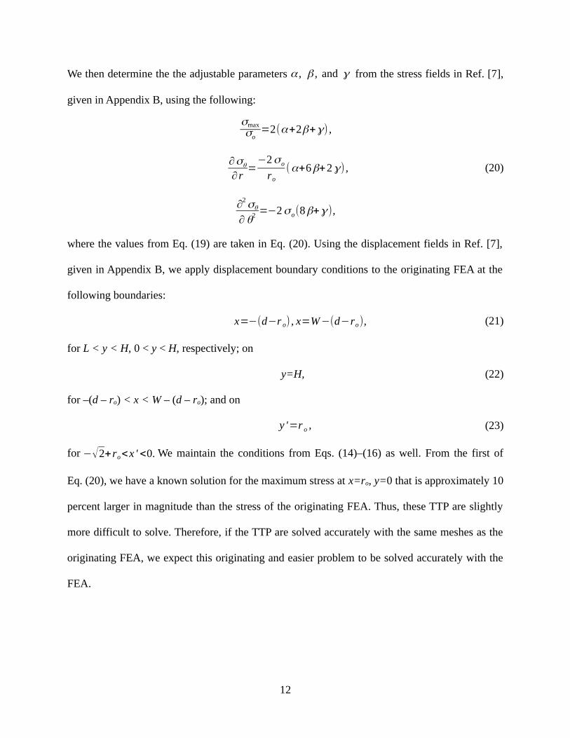
We then determine the the adjustable parameters α , β , and γ from the stress fields in Ref. [7],

given in Appendix B, using the following:

σmaxσo

=2(α+2β+γ) ,

∂σθ

∂r=

−2σo

ro

(α+6β+2γ) , (20)

∂2σθ

∂ θ2 =−2σ o(8β+γ),

where the values from Eq. (19) are taken in Eq. (20). Using the displacement fields in Ref. [7],

given in Appendix B, we apply displacement boundary conditions to the originating FEA at the

following boundaries:

x=−(d−r o) , x=W−(d−ro), (21)

for L < y < H, 0 < y < H, respectively; on

y=H, (22)

for –(d – ro) < x < W – (d – ro); and on

y '=r o , (23)

for −√2+ro<x ' <0. We maintain the conditions from Eqs. (14)–(16) as well. From the first of

Eq. (20), we have a known solution for the maximum stress at x=ro, y=0 that is approximately 10

percent larger in magnitude than the stress of the originating FEA. Thus, these TTP are slightly

more difficult to solve. Therefore, if the TTP are solved accurately with the same meshes as the

originating FEA, we expect this originating and easier problem to be solved accurately with the

FEA.

12

4. Results for Peak Notch Stresses

In Sec. 3, we describe our methodology to verify that finite width and height dimensions

do not result in changes to the maximum stress at the notch root. To demonstrate this process in

our choice of W and H, we consider the least acute notch, ro/L=1/32, and review the maximum

stress at the notch root, x=ro, y=0, as the height and width increases. We select the least acute

notch because this notch has elevated stresses distributed over the largest fraction of the net-

section width. As a result, this notch will require the most substantial width increases before the

behavior is essentially the same as a semi-infinite plate. Consequently, we expect that the

necessary width for the least acute notch will be sufficient for more acute notches.

Table 2 shows the result of the finest mesh of ro/L=1/32 for the normalized maximum

stress as we double the net-section width, taking it equal to a×(W-d), where a=1, 2, 4, 8. We

initialize the width as W=2L, so the initial net-section is (2L-d). We maintain a constant height,

H=L. As the width increases from a=4 to a=8, the maximum normalized result is the same to six

figures, so we take the net-section width as four times its initial value, leading to the expression

for W/L in Eq. (18). In a similar fashion, we now double the height for this selected width. Table

3 shows the maximum normalized stress at the notch root for ro/L=1/32 as the height increases,

starting with H=2L. Upon a height increase from H=8L to 16L, the result for maximum stress at

the notch root is the same to five figures. Thus, we take the height as H=8L, completing the

specification given in Eq. (18).

Table 2. Normalized maximum stress for ro/L=1/32 upon doubling net-section width (H=L)

13

a1 34.19672 28.63764 28.57778 28.5777

Table 3. Normalized maximum stress for ro/L=1/32 upon doubling height

We conduct the same procedure for ro/L=1/512 and see similar behavior as the plate

dimensions Table 7 increase. Upon reaching a net-section width that is four times the initial net

section, the normalized maximum stress from the finest mesh is constant to five figures upon a

subsequent doubling. Likewise, the upon reaching a height of H/L=8, the normalized maximum

stress is constant to five figures upon doubling to H/L=16. Thus, as we construct all of the

remaining, more acute notches, we take a width that is four times the initial net section and a

height that is H/L=8.

We consider ro/δ=2.06 as a representative case to review results for verification because

this configuration produces the largest normalized stress at the notch root with uniformly applied

cohesive laws. Figure 5(a) shows the normal stress along the symmetry line y=0. At the scale of

Fig. 5(a), the results from different meshes are indistinguishable. Figure 5(b) shows the results in

detail near the notch root for each FEA mesh. As the meshes refine, the results begin to overlap

as they approach the same solution.

14

H/L2 18.61704 15.87838 15.794516 15.7944

Fig. 5. (a) Normal stress along y=0 for ro/δ=2.06, (b) detailed results near notch tip

To check for convergence, we let σm denote , and denote the increment

accompanying mesh refinement as Δσm=σm−σm−1 . We say that a mesh is converging if Δσm is

reducing for each mesh refinement and that Δσm is the same sign. That is,

Δσm<Δσm−1 ,Δσm×Δσm−1>1 ,

(24)

must be true for convergence to occur. When the convergence criteria in Eq. (24) are satisfied for

a given mesh and m≥2, we calculate the estimated convergence rate using

, (25)

where λm=Nm/Nm-1. If the convergence criteria are satisfied and m≥3, we calculate the estimated

error (in percent) using

15

(a) (b)

εm=Δ σm

σm (λmcm−1 )

×100. (26)

For further details, see Ref. [6].

We apply the traction σo such that the peak stress at the notch root is within one percent of

the ultimate stress, effectively determining the maximum stress concentration for a particular

notch configuration. Table 4 shows the FEA results for ro/δ=2.06 with uniform cohesive laws

applied. Convergence does not occur initially, but the conditions in Eq. (24) are satisfied for m=4

and 5. In order to calculate Δσm to three figures, we keep σm to seven figures. The error estimate

is below our 1/5 percent threshold in m=4. However, we compute results for one finer mesh,

m=5, as an assurance that the FEA continues to converge with further mesh refinement, and

accept the result from m=5 as sufficiently accurately determined. This converged result is 99.2

percent of the ultimate stress.

Table 4. Finite element values of with uniform cohesive laws for ro/δ=2.06

Results for global meshes for other notch radii with cohesive laws active are given in

Appendix C. These results consistently have converging error estimates that are below 1/5

percent, with one exception for ro/δ=0, which approaches 1/5 percent.

As further verification of our FEA, we consider results from symmetry conditions and the

TTP for ro/δ=2.06. Table 5 contains the normalized maximum stress results from symmetry

boundary conditions. An additional mesh, m=6, is used for the symmetry conditions and the

TTP. This mesh contains 4,147,566 elements. From Table 5, we see the FEA begins to converge

16

m (%)1 13893.18 - - -2 13806.16 -87.02 - -3 13715.64 -90.52 - -4 13690.60 -25.04 1.85 0.075 13685.35 -5.25 2.25 0.01

σm Δσ

mεm

from m=3 to m=4. The estimated error in m=6 is below 1/5 percent, and is therefore judged to be

sufficiently accurately determined. We proceed to construct a TTP from this result.

Table 5. Finite element values of with symmetry conditions for ro/δ=2.06

Using the results from the FEA, we determine the values specified in Eq. (19) and find

the parameters in (20) to be

α=4,962.5 , β=2,260.0 , γ=7,564.5 , (27)

with an exact value for =34,094, 10 percent higher than in Table 5. The values in Eq.

(27) are also exact and contain no additional figures. Using the parameters in Eq. (27) in the

displacement fields given in Appendix B, we solve the same meshes as the originating FEA to

determine the TTP results in Table 6. Table 6 also contains the true convergence rate and the true

error, given as cm and εm , respectively.

Table 6. Finite element values of for the TTP with ro/δ=2.06 (exact = 34,094)

17

m1 30,428.1 - - -2 30,516.7 88.6 - -3 30,723.4 206.7 - -4 30,867.5 144.1 0.52 1.15 30,949.9 82.4 0.81 0.366 30,993.6 43.7 0.92 0.16

σm Δσ

m εm (%)

m (%)1 32,627.9 - 4.3 - - -2 33,333.5 0.95 2.2 705.6 - -3 33,706.0 0.97 1.1 372.5 0.92 1.24 33,897.9 0.98 0.58 191.9 0.96 0.605 33,995.4 0.99 0.29 97.5 0.98 0.306 34,044.6 1.00 0.14 49.2 0.99 0.15

σm Δσ

mcmεm (%) εm

The results for the TTP in Table 6 begin to converge immediately. The true convergence

rate cm steadily approaches the asymptotic limit of 1 for 4Q elements as the mesh refines,

eventually reaching 1.00 due to rounding. We accept the result from m=6 as being accurately

determined. Where comparison may occur, the estimated error is conservative, but nonetheless

tracks the true error well.

Both the FEA and TTP reach an estimated error below 1/5 percent. This TTP

demonstrates that the mesh structure for this notch can accurately determine a peak stress that is

much larger than that of Table 4. Therefore, we expect that the FEA with uniform cohesive laws

is solved accurately as well.

Results for other TTP, specifically for the notches given by Eq. (12) are provided in

Andrus and Sinclair [8]. The FEA and accompanying TTP for these notches consistently

converge to an error level that is below 1/5 percent.

With the cohesive laws removed completely from the notch face, we obtain larger values

of than with uniformly applied cohesive laws. We select ro/δ=0.00402 as the case to

review results obtained with partially applied cohesive laws since this configuration produces the

largest result for obtained by FEA. Table 7 contains FEA results for ro/δ=0.00402. Details

for the mesh refinement sequence are given in Appendix A.

Table 7. Finite element values of with cohesive laws removed from notch face for ro/δ=0.00402

18

m (%)1 35126.7 - - -2 34333.0 -793.7 - -3 34127.4 -205.6 1.95 0.214 34075.1 -52.3 1.97 0.05

σm

Δσm

εm

The FEA results in Table 7 begin to converge immediately. The result for m=4 is below the 1/5

percent threshold, and so we accept this result as sufficiently accurately determined.

Appendix D contains additional FEA results for the notch radii given by Eq. (13) with

p=11–14. The FEA for each notch converges below the 1/5 percent threshold. We use the results

in Appendix D to extrapolate a result for ro/δ=0 of =34,170.8, which we judge to be

sufficiently accurately determined. Appendix E contains details for the extrapolation procedure.

Regarding the physical implications of these results, we note that a different choice of

material and cohesive laws will have some influence on the result. However, we expect that

results for other similar materials and cohesive laws will produce a similar trend to the results

here.

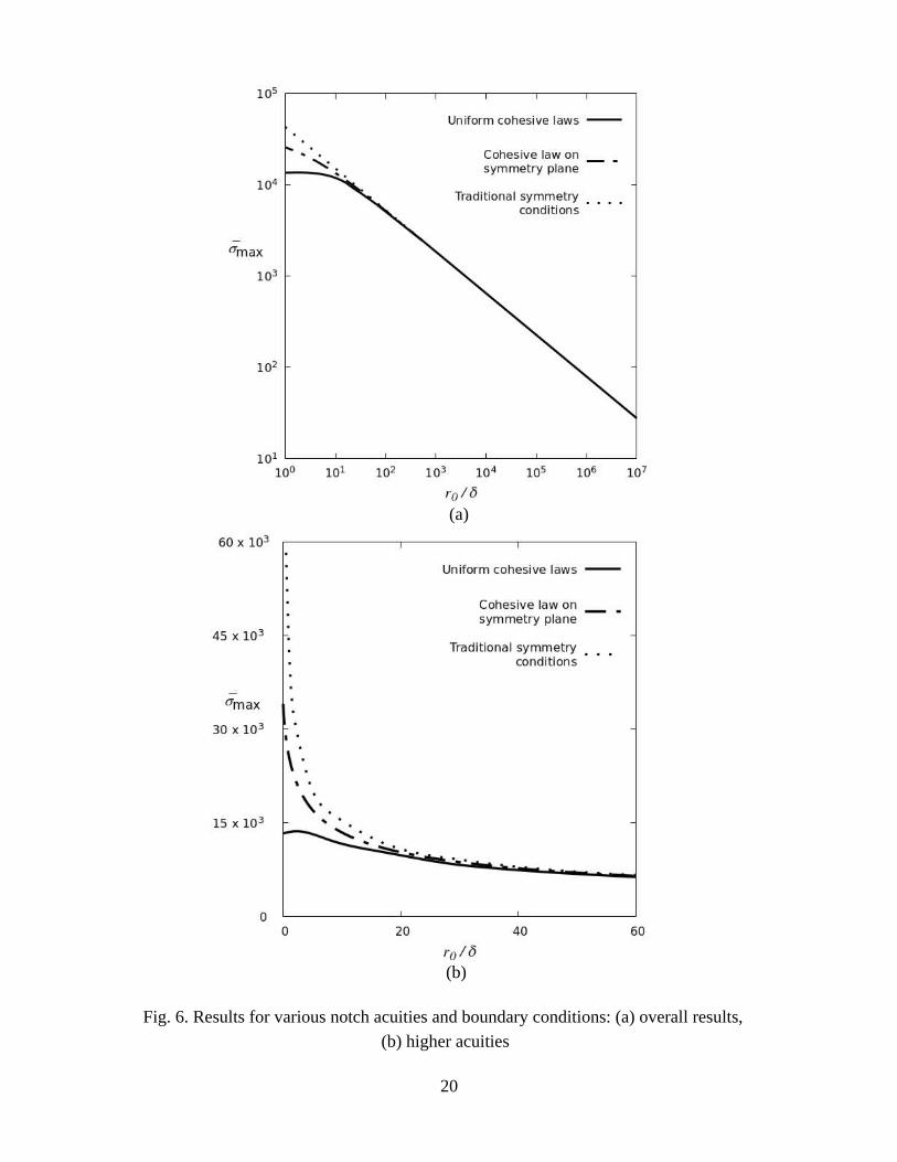
Figure 6 shows the results of for each notch configuration given by Eqs. (12) and

(13) with the various boundary conditions. It is readily apparent in Fig. 6(a) that for large radii,

the cohesive laws yield the same results as the traditional symmetry conditions. Figure 6(b)

shows results for the smaller radii of Eq. (13). The results with uniformly applied cohesive laws

reach a finite value for the case of ro/δ=0 and a maximum at ro/δ=2. The results with the

cohesive laws on only the symmetry plane are elevated compared to the uniform cohesive laws,

but still finite. Figure 6(b) also indicates more clearly that peak stresses with traditional

symmetry conditions are singular as the notch radius tends to zero.

19

20

(a)

(b)

Fig. 6. Results for various notch acuities and boundary conditions: (a) overall results,

(b) higher acuities

The results for for traditional symmetry conditions agree well with the results for

uniformly applied cohesive laws when ro/δ is larger than approximately 500. For more acute

radii, the results begin to deviate. When ro/δ=66, the difference is within five percent. When

ro/δ=30, the difference is about 10 percent. When ro/δ=2, where we obtain the largest normalized

stress from uniformly applied cohesive laws, the difference is about 126 percent. It is evident that

traditional symmetry conditions are applicable for a broad range of radii and the singular nature

of the symmetry conditions is not pronounced until the notch is very acute.

The results for for cohesive laws on the symmetry plane also agree with the results

for uniformly applied laws for a broad range of radii. The difference between results for these

boundary conditions is within one percent when ro/δ=500. For a notch size of ro/δ=30, the

difference is within five percent. When ro/δ=2, the difference is approximately 61 percent. For

the sharp corner, ro/δ=0, the difference between the results is approximately 156 percent.

In Table 8, we present the results for for each boundary condition for the

following notch configurations: ro/δ=500, 30, 2, 0. We select ro/δ=500 and 30 because these are

the acuities where we see a negligible difference and a 10 percent difference, respectively,

between symmetry conditions and cohesive laws. We pick ro/δ=2 because we find the maximum

with cohesive laws at this notch acuity. Lastly, we select the sharp corner to present the

finite stress results.

Table 8. Selected results for with different boundary conditions

21

500 2,524 2,531 2,53830 8,292 8,747 9,1432 13,685 22,019 30,9940 13,323 34,171 ∞

ro/δ Uniform cohesive

lawsPartial

cohesive laws

Traditional symmetry conditions

5. Concluding Remarks

In this thesis, we consider a semi-infinite elastic plate with a 90-degree V-notch in one

side and seek the peak stress at the notch tip as the notch radius approaches zero. As our

principal focus, we seek results by implementing cohesive stress-separation laws on the notch

face and symmetry plane between the upper and lower halves of the plate. We further seek

results with cohesive laws applied only to the symmetry plane with stress free conditions on the

notch face. Lastly, we consider results from traditional symmetry boundary conditions on the

symmetry plane with stress-free conditions on the notch face.

We use FEA to conduct the analysis of these notch problems. We verify our FEA results

with convergence checks and constructed test problems (TTP). This verification indicates that all

reported results approach 1/5 percent accuracy or less.

The key conclusion from these results is that for a 90-degree V-notch with uniformly

applied cohesive laws, the largest peak stress does not occur for the sharp corner, but rather for a

notch radius of ro/δ=2, where ro is the local notch radius and δ is the equilibrium separation

between atoms. We find this peak stress to be σmax /σo=13,700 , where σmax is the peak stress at

the notch tip and σo is an applied farfield traction. With the cohesive laws applied on only the

symmetry plane, we find that as ro tends to zero, peak stress results are larger than those with

uniformly applied cohesive laws. For the partially applied laws, the peak stress result reaches a

maximum of σmax /σo=34,100 when ro/δ=0, which is a sharp corner. Results from traditional

symmetry conditions agree with the uniform cohesive laws for notch radii greater than ro/δ=500.

The results from symmetry conditions are about 10 percent higher than the uniform cohesive

laws for a notch radius of ro/δ=30.

22

Appendix A. Finite Element Meshes

Mesh structure for notches with greater acuity, such as those in Eq. (13), are shown in the

text in Fig. 4. Notches with less acuity, as in Eq. (12), have a mesh structure that is illustrated in

Fig. 7. The mesh in Fig. 7 is less refined since these notches have lower peak stresses at the

notch root.

Fig. 7. Mesh m=1 for ro/L=1/32: (a) farfield mesh, (b) detail near notch tip

Table 9 contains mesh sequences for these less refined meshes. To assess convergence,

we use an element refinement factor of two. We halve element extents in the structured regions,

strictly quadrupling elements in these regions. The element extent on the notch, hm/ro on r=ro, for

all of the configurations in Table 9 are 1/10.2, 1/20.4, 1/40.8, 1/81.6, 1/163. In the unstructured

regions, we approximately quadruple the element counts, thus halving the element extents on

average. This increases the overall number of elements Nm by close to a factor of four for each

successive refinement, as seen in Table 9.

23

(b)

(a)

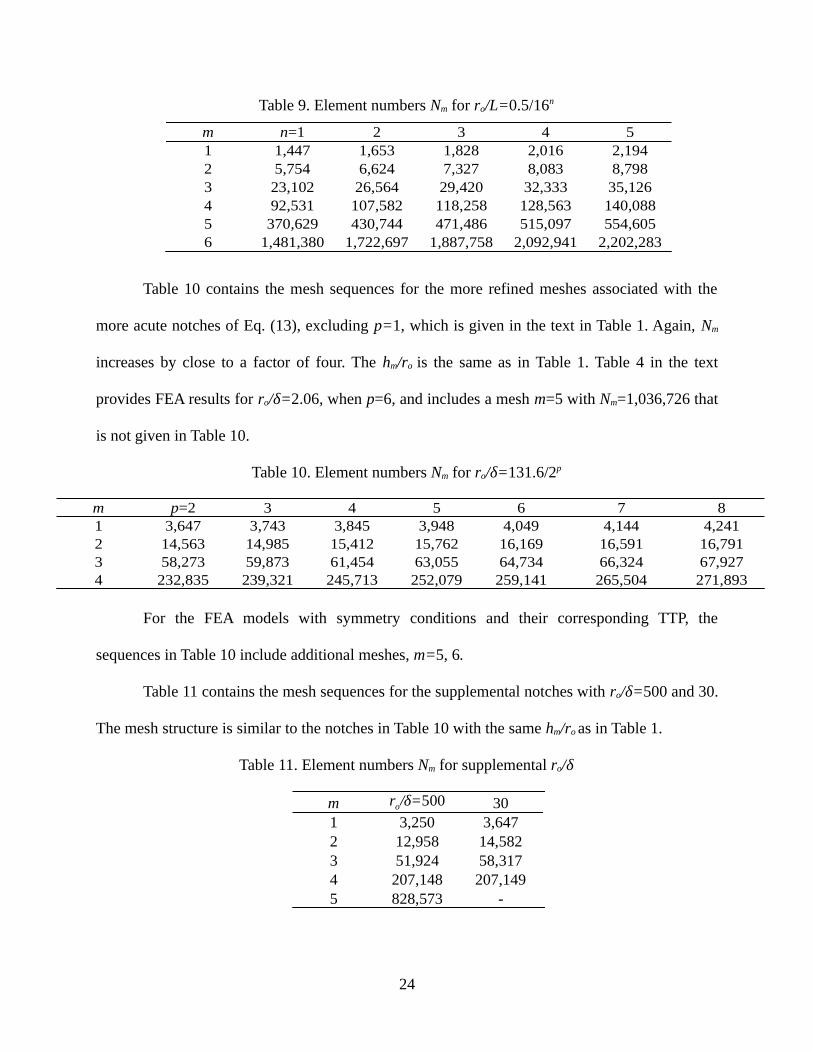
Table 9. Element numbers Nm for ro/L=0.5/16n

Table 10 contains the mesh sequences for the more refined meshes associated with the

more acute notches of Eq. (13), excluding p=1, which is given in the text in Table 1. Again, Nm

increases by close to a factor of four. The hm/ro is the same as in Table 1. Table 4 in the text

provides FEA results for ro/δ=2.06, when p=6, and includes a mesh m=5 with Nm=1,036,726 that

is not given in Table 10.

Table 10. Element numbers Nm for ro/δ=131.6/2p

For the FEA models with symmetry conditions and their corresponding TTP, the

sequences in Table 10 include additional meshes, m=5, 6.

Table 11 contains the mesh sequences for the supplemental notches with ro/δ=500 and 30.

The mesh structure is similar to the notches in Table 10 with the same hm/ro as in Table 1.

Table 11. Element numbers Nm for supplemental ro/δ

24

m 2 3 4 51 1,447 1,653 1,828 2,016 2,1942 5,754 6,624 7,327 8,083 8,7983 23,102 26,564 29,420 32,333 35,1264 92,531 107,582 118,258 128,563 140,0885 370,629 430,744 471,486 515,097 554,6056 1,481,380 1,722,697 1,887,758 2,092,941 2,202,283

n=1

m 3 4 5 6 7 81 3,647 3,743 3,845 3,948 4,049 4,144 4,2412 14,563 14,985 15,412 15,762 16,169 16,591 16,7913 58,273 59,873 61,454 63,055 64,734 66,324 67,9274 232,835 239,321 245,713 252,079 259,141 265,504 271,893

p=2

m 301 3,250 3,6472 12,958 14,5823 51,924 58,3174 207,148 207,1495 828,573 -

ro/δ=500

Table 12 contains the mesh sequences for the additional notches used in the limiting case

where the cohesive laws on the notch face are removed. The mesh structure is similar to the

notches in Table 10, and again Nm increases by close to a factor of four. The hm/ro is the same as

in Table 1.

Table 12. Element Numbers Nm for ro/δ=131.6/2p

25

m 12 13 14 151 4,535 4,655 4,742 4,851 4,9492 18,173 18,578 18,981 19,388 19,7813 72,715 74,322 75,964 77,434 79,0744 291,062 297,535 303,934 309,547 315,958

p=11

(b)(c)

(a)

Fig. 8. Mesh m=1 for ro/δ =0: (a) farfield, (b) structured mesh detail, (c) detail near notch tip

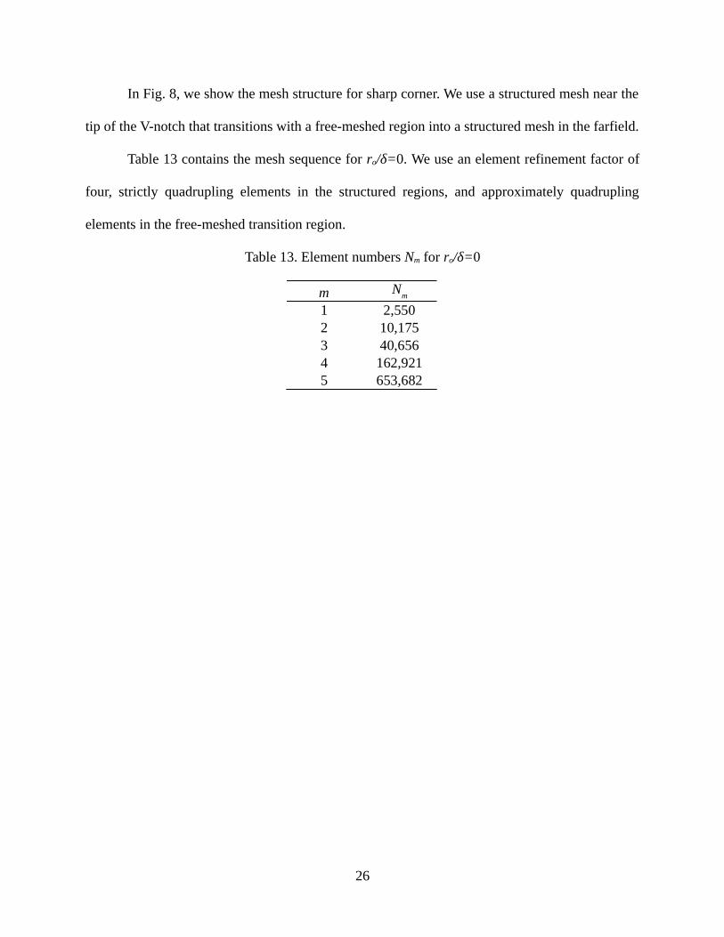
In Fig. 8, we show the mesh structure for sharp corner. We use a structured mesh near the

tip of the V-notch that transitions with a free-meshed region into a structured mesh in the farfield.

Table 13 contains the mesh sequence for ro/δ=0. We use an element refinement factor of

four, strictly quadrupling elements in the structured regions, and approximately quadrupling

elements in the free-meshed transition region.

Table 13. Element numbers Nm for ro/δ=0

26

m1 2,5502 10,1753 40,6564 162,9215 653,682

Nm

Appendix B. Fields for Tuned Test Problems

The following fields are from Ref. [7]. The stresses satisfy the stress equations of

equilibrium and compatibility, and they have zero stress on r=ro:

σr=σo[α(1−ro

2

r2 )−β(1+3ro

4

r4 −4ro

2

r2 )cos2θ+γ ro

r (1−ro

2

r2 )cosθ ] ,

σθ=σo[α(1+ro

2

r2 )+β(1+3ro

4

r4 )cos2θ+γ ro

r (1+ro

2

r2 )cosθ ] ,

τ rθ=σo[β(1−3r o

4

r 4 +2ro

2

r2 )sin 2θ+γ ro

r (1−ro

2

r2 )sin θ] .Their companion displacements satisfy the stress-displacement relations for a homogeneous,

isotropic, linear, elastic solid in a state of plane strain:

ur=σo[2α ((1−2ν)r+ro

2

r )−2β(r+4(1−ν)ro

2

r−

ro4

r3 )cos2θ

+γ r 0((2 (1−ν) lnrr o

−1+ro

2

r 2 )cos θ+4 (1−ν)θsin θ)]/ 4μ ,

uθ=σo[2β(r+2(1−2ν)ro

2

r−

ro4

r3 )sin 2θ

−γ r0((2(1−2ν) lnrr o

+1−r o

2

r2 )sinθ−4(1−ν)θcos θ)]/4μ .

27

Appendix C. Convergence Checks for Maximum Stresses with Uniform Cohesive Laws

The tables in this appendix provide detailed results from FEA with cohesive laws

uniformly applied for the following notch configurations: ro/L=0.5/16n for n=1, 3, 5, and

ro/δ=131.6/2p for p=2, 4, 8. For the less acute notches, n=1, 3, 5, the results with cohesive laws

are the same as with traditional symmetry conditions. Tables 14–16 contain results for the less

acute notches where n=1, 3, 5, and Tables 17–19 contain results for the more acute notches

where p=2, 4, and 8. Table 20 includes the result for ro/δ=0.

Table 14. Finite element values of for ro/L= 0.5/16

Table 15. Finite element values of for ro/L= 0.5/163

Table 16. Finite element values of for ro/L= 0.5/165

28

m (%)1 15.1121 - - -2 15.4496 0.3375 - -3 15.6313 0.1817 0.89 1.44 15.7239 0.0926 0.97 0.615 15.7708 0.0469 0.98 0.316 15.7945 0.0237 0.99 0.15

σm

Δσm εm

m (%)1 190.074 - - -2 194.013 3.939 - -3 196.246 2.233 0.82 1.54 197.393 1.147 0.96 0.615 197.980 0.587 0.96 0.316 198.274 0.294 1.00 0.15

σm

Δσm εm

m (%)1 2366.77 - - -2 2418.73 51.96 - -3 2447.27 28.54 0.86 1.44 2461.44 14.17 1.01 0.575 2468.54 7.10 1.00 0.296 2472.01 3.47 1.04 0.13

σm

Δσm εmεm

Table 17. Finite element values of for ro/δ=32.9

Table 18. Finite element values of for ro/δ=8.23

Table 19. Finite element values of for ro/δ=0.514

Table 20. Finite element values of for ro/δ=0

29

m (%)1 8206.82 - - -2 8062.87 -143.95 - -3 8025.36 -37.51 1.94 0.164 8017.96 -7.40 2.34 0.02

σm

Δσm εmεm

m (%)1 12540.3 - - -2 12266.4 -273.9 - -3 12190.1 -76.3 1.85 0.244 12175.8 -14.3 2.42 0.12*

σm

Δσm εmεm

m (%)1 13547.92 - - -2 13534.43 -13.49 - -3 13492.41 -42.02 - -4 13454.29 -38.12 0.14 2.775 13444.90 -9.39 2.02 0.07*

σm

Δσm εmεm

m (%)1 14760.1 - - -2 14007.4 -752.7 - -3 13564.4 -443.0 - -4 13383.7 -180.7 1.29 0.935 13323.0 -60.7 1.57 0.23

σm

Δσm εmεm

Results for estimated errors in Tables 14–19 consistently converge below 1/5 percent.

Results for intermediary notch sizes likewise converge with estimated errors below 1/5 percent.

The result in Table 20 for ro/δ=0 approaches an estimated error of 1/5 percent. The results

denoted with an asterisk are calculated by taking =1.0 to avoid significantly underestimating

the error when the convergence rates increase significantly: this is done in accordance with the

modified convergence estimates of Beisheim et al. [9].

30

Appendix D. Convergence Checks for Maximum Stresses with Cohesive Laws on Symmetry Plane

The tables in this appendix provide detailed results from FEA with cohesive laws applied

to only the symmetry plane for the following notch configurations: ro/δ=131.6/2p for p=11, 12,

13, 14. Tables 21–24 provide results for these notches in order of increasing notch acuity.

Table 21. Finite element values of for ro/δ=0.0643

Table 22. Finite element values of for ro/δ=0.0321

Table 23. Finite element values of for ro/δ=0.0161

Table 24. Finite element values of for ro/δ=0.00803

31

m (%)1 34067.2 - - -2 33251.0 -816.2 - -3 33044.3 -206.7 1.98 0.634 32989.8 -54.5 1.92 0.17

σm

Δσm

εm

m (%)1 34563.9 - - -2 33780.6 -783.3 - -3 33573.8 -206.8 1.92 0.224 33520.0 -53.8 1.94 0.06

σm

Δσm

εm

m (%)1 34871.8 - - -2 34081.9 -789.9 - -3 33873.0 -208.9 1.92 0.224 33820.2 -52.8 1.98 0.05

σm

Δσm

εm

m (%)1 35030.6 - - -2 34244.6 -786.0 - -3 34038.0 -206.6 1.93 0.224 33985.4 -52.6 1.97 0.05

σm

Δσm

εm

Each FEA converges below the 1/5 percent threshold when m=4, so we accept these

results as being sufficiently accurately determined.

32

Appendix E. Peak Stress Results with ro=0 with Cohesive Laws on the Symmetry Plane

Determining a consistent result through FEA for ro/δ=0 with the cohesive laws removed

from the notch face proved challenging due to implementation of the COMBIN39 spring element

at the sharp corner. When the notch has a nonzero radius, we obtain consistent results through

FEA with the spring elements removed from the notch face, and so choose to extrapolate a result

for ro/δ=0.

We create increasingly acute notches beyond those given in the text with Eq. (13) to

include notch configurations for p=11, 12, …, 15. The smallest notch configuration created with

cohesive laws removed from the notch face is ro/δ=0.00402. We use converged results from

these notches for our extrapolation procedure, shown next.

Extrapolation proceeds with

K=K o−Δ K 1( Rr o

)+Δ K2( Rro

)2

−Δ K3( Rro

)3

, (28)

where Ko, ΔK1, ΔK2, and ΔK3 are constants, K= and is determined with FEA, R is the

corresponding notch radius for an accompanying K, and ro is a reference radius. We test this

method by extrapolating a result for ro/δ=0.00402 and comparing it to the FEA result.

Table 25 shows the results for from the finest mesh of each notch for p=11–15.

Table 25. Finite element results for ro/δ=131.6/2p with partially applied cohesive laws and p=11, 12, … , 15

33

32,989.812 33,520.013 33,820.214 33,985.415 34,075.1

ro/δ=131.6/2p

p=11

Each increase of p causes ro to decrease by exactly half, so taking the results for p=11–15 from

Table 25, we solve the following system of equations:

32,989.8=K o−Δ K1+ΔK 2−Δ K 3 , (29)

33,520.0=K o−Δ K1

2+

Δ K2

4−

Δ K3

8, (30)

33,820.2=Ko−Δ K1

4+

Δ K2

16−

Δ K3

64, (31)

33,985.4=K o−Δ K1

8+

Δ K2

64−

ΔK 3

512, (32)

and find K o=34,163.07619, Δ K1=1,476.133333 , Δ K2=457.0666667 , and

Δ K3=154.2095238 . Substituting the foregoing results into Eq. (28), we determine K=34,072.6

for ro/δ=0.00402, which is within 0.01 percent of the FEA result in Table 7. Thus, we conclude

that the extrapolation procedure works well and use it to determine a result for ro/δ=0.

34

References

[1] Williams, M. L., 1952, “Stress Singularities Resulting from Various Boundary Conditions in Angular Corners of Plates in Extension,” ASME J. Appl. Mech., 19, pp. 526-528.

[2] Sinclair, G. B., 1996, “On the Influence of Cohesive Stress-Separation Laws on Elastic Stress Singularities,” J. Elasticity, 44, pp. 203-221.

[3] Sinclair, G. B., Meda, G., and Smallwood, B. S., 2011, “On Crack-Tip Stresses as Crack-Tip Radii Decrease,” ASME J. Appl. Mech., 78, p. 011004.

[4] Cherepanov, G. P., 1979, Mechanics of Brittle Fracture, McGraw-Hill, New York.

[5] ANSYS, 2018, “ANSYS Mechanical APDL Element Reference,” Release 19.1, ANSYS Inc., Canonsburg, PA.

[6] Sinclair, G. B., Beisheim, J. R., and Roache, P. J., 2016, “Effective Convergence Checks for Verifying Finite Element Stresses at Two-Dimensional Stress Concentrations,” ASME J. Verif. Valid. Uncert. Quant., 1, p. 041003.

[7] Sinclair, G. B., Anaya-Dufresne, M., Meda, G., and Okajima, M., 1998, “Tuned Test Problems for Numerical Methods in Engineering,” Int. J. Numer. Methods Eng., 40, pp. 4183-4209.

[8] Andrus, T. M., and Sinclair, G. B., 2020, “Verification of Finite Element Analysis for the Stress Concentrations Occurring at V-Shaped Notches Using Tuned Test Problems,” Report No. ME-MS2-20, Department of Mechanical Engineering, Louisiana State University.

[9] Beisheim, J. R., Sinclair, G. B., and Bilich, L. A., 2015, “Convergence Checks in the Presence of Nonmonotonic Convergence,” Proc. NAFEMS World Congress, San Diego, CA, on CD-ROM.

35

Vita

Trent Andrus was born and raised in Lafayette, Louisiana. Trent attended Louisiana State

University for his Bachelor of Science in Mechanical Engineering and graduated in 2018 with

Upper Division Honors Distinction from the Roger Hadfield Ogden Honors College. While at

LSU for his undergraduate degree, Trent participated in the SpaceX Hyperloop Design

Competition, founded a student organization focused on environmental issues, and completed a

photo-documentary project entitled Louisiana Gone with a colleague using funds from the Roger

Hadfield Ogden Honors College. Louisiana Gone was entered in the 2017 LSU Discover Day

Juried Art Show, where it was awarded "Tiger's Choice" as a fan-favorite. Trent continued his

education at LSU, beginning a Master of Science for Mechanical Engineering in 2018 and

anticipates graduation in Fall 2020. Trent conducted research using finite element analysis

software for his undergraduate and graduate degrees. During his Master's, Trent interned at

Ansys, where he now works full-time as a R&D Verification Engineer.

36