on the stability of periodic solutions in the perturbed ...malisoff/papers/ams-slides.pdf · on the...
TRANSCRIPT

On the Stability of Periodic Solutionsin the Perturbed Chemostat
MICHAEL MALISOFFDepartment of MathematicsLouisiana State University
Joint work withFrederic Mazenc(INRIA-INRA)andPatrick De Leenheer(University of FL)
SIAM Minisymposium on Mathematical Modelingof Complex Systems in Biology I
AMS Joint Meetings, New Orleans, LA, January 6, 2007
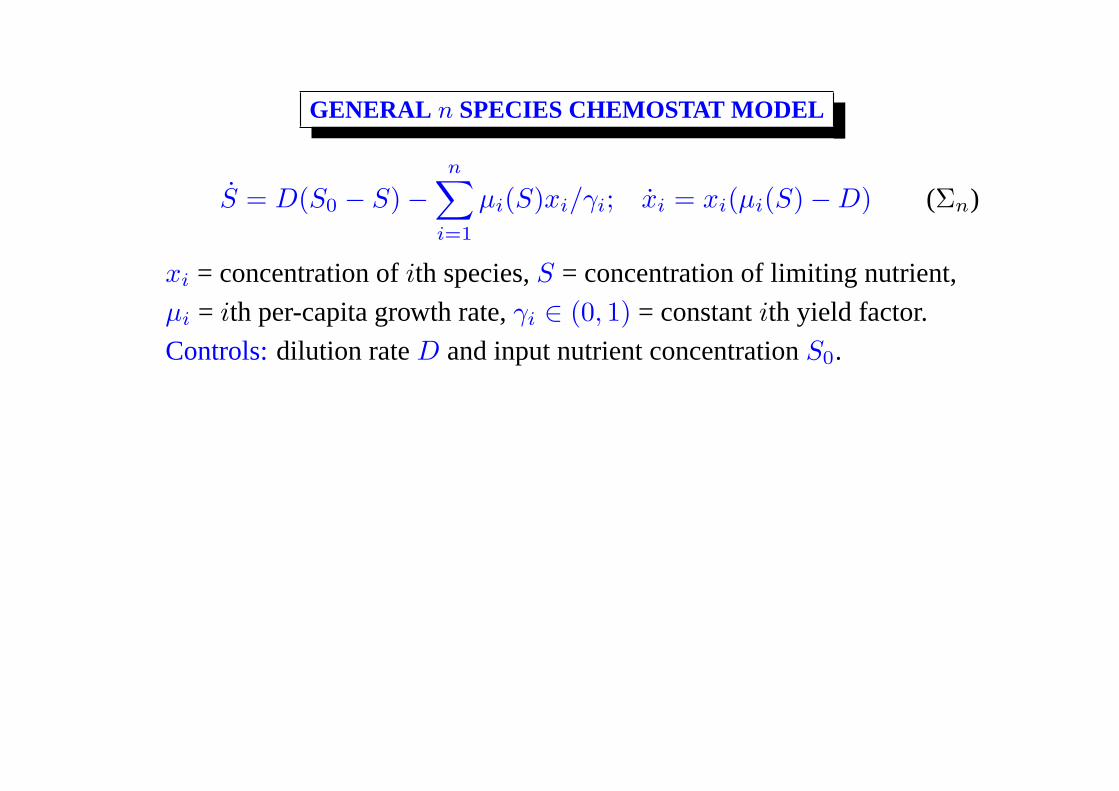
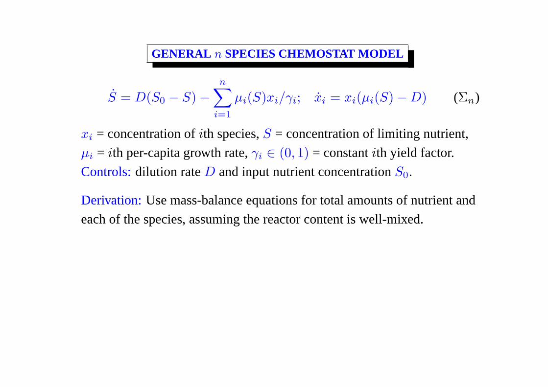
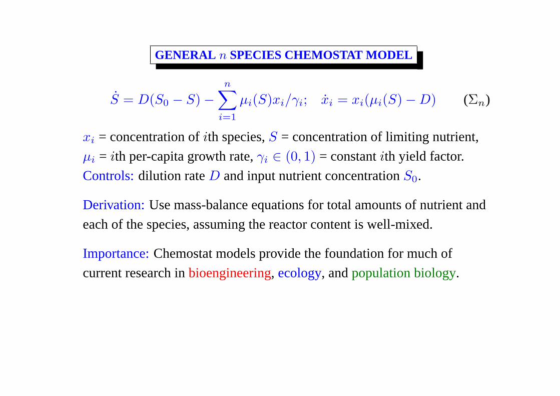
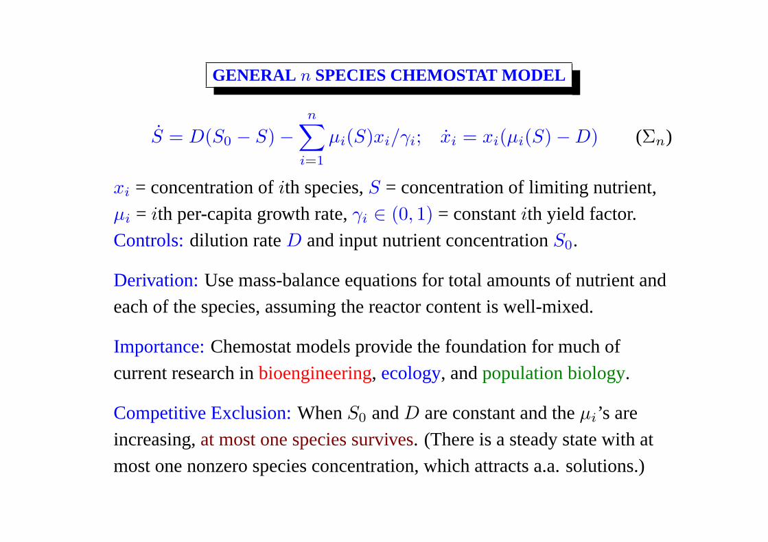
GENERAL n SPECIES CHEMOSTAT MODEL
S = D(S0 − S)−n∑
i=1
µi(S)xi/γi; xi = xi(µi(S)−D) (Σn)
xi = concentration ofith species,S = concentration of limiting nutrient,
µi = ith per-capita growth rate,γi ∈ (0, 1) = constantith yield factor.
Controls:dilution rateD and input nutrient concentrationS0.
GENERAL n SPECIES CHEMOSTAT MODEL
S = D(S0 − S)−n∑
i=1
µi(S)xi/γi; xi = xi(µi(S)−D) (Σn)
xi = concentration ofith species,S = concentration of limiting nutrient,
µi = ith per-capita growth rate,γi ∈ (0, 1) = constantith yield factor.
Controls:dilution rateD and input nutrient concentrationS0.
Derivation:Use mass-balance equations for total amounts of nutrient and
each of the species, assuming the reactor content is well-mixed.
Importance:Chemostat models provide the foundation for much of
current research inbioengineering, ecology, andpopulation biology.
Competitive Exclusion:WhenS0 andD are constant and theµi’s are
increasing,at most one species survives. (There is a steady state with at
most one nonzero species concentration, which attracts a.a. solutions.)

OVERVIEW of LITERATURE
Coexistence:In real ecological systems,many species can coexist, so
much of the literature aims at choosingS0 and/orD to force coexistence.
“The Paradox of the plankton,” Hutchinson,American Naturalist, 1961.

OVERVIEW of LITERATURE
Coexistence:In real ecological systems,many species can coexist, so
much of the literature aims at choosingS0 and/orD to force coexistence.
“The Paradox of the plankton,” Hutchinson,American Naturalist, 1961.
Time-Varying Controls:Have competitive exclusion ifn = 2 and one of
the controls is fixed and the other is periodic. See Hal Smith (SIAP’81),
Hale-Somolinos (JMB’83), Butler-Hsu-Waltman (SIAP’85).
State-Dependent Controls:A feedback control perspective based on
mathematical control theorywas pursued e.g. in De Leenheer-Smith
(JMB’03) to generate a coexistence equilibrium forn = 2, 3.
Intra-Specific Competition:This can be modeled with growth rates
µi(S, xi) that decrease inxi. See Mazenc-Lobry-Rapaport (EJDE’07),
Grognard-Mazenc-Rapaport (DCDS’07).

OUR WORK for ONE SPECIES CASE
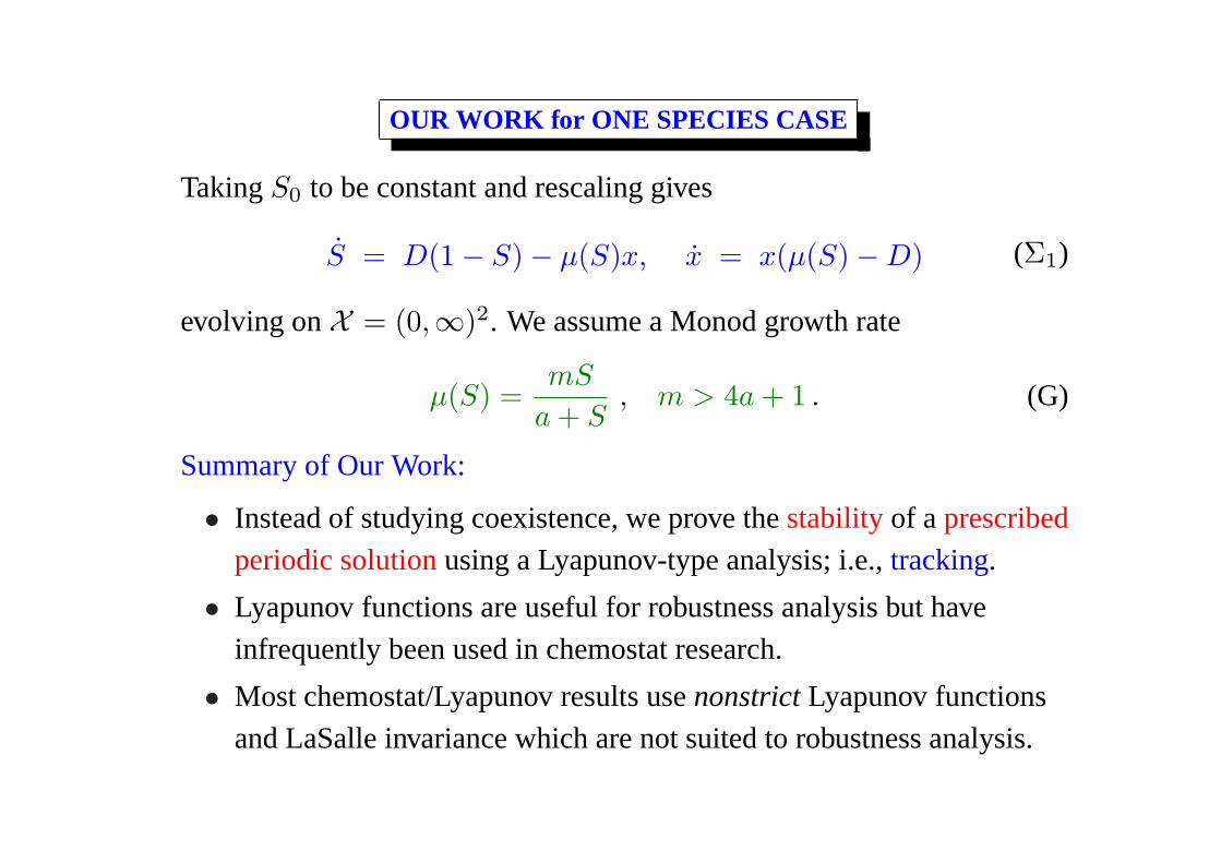
TakingS0 to be constant and rescaling gives
S = D(1− S)− µ(S)x, x = x(µ(S)−D) (Σ1)
evolving onX = (0,∞)2. We assume a Monod growth rate
µ(S) =mS
a + S, m > 4a + 1 . (G)

OUR WORK for ONE SPECIES CASE
TakingS0 to be constant and rescaling gives
S = D(1− S)− µ(S)x, x = x(µ(S)−D) (Σ1)
evolving onX = (0,∞)2. We assume a Monod growth rate
µ(S) =mS
a + S, m > 4a + 1 . (G)
Summary of Our Work:
• Instead of studying coexistence, we prove thestabilityof aprescribed
periodic solutionusing a Lyapunov-type analysis; i.e.,tracking.
• Lyapunov functions are useful for robustness analysis but have
infrequently been used in chemostat research.
• Most chemostat/Lyapunov results usenonstrictLyapunov functions
and LaSalle invariance which are not suited to robustness analysis.
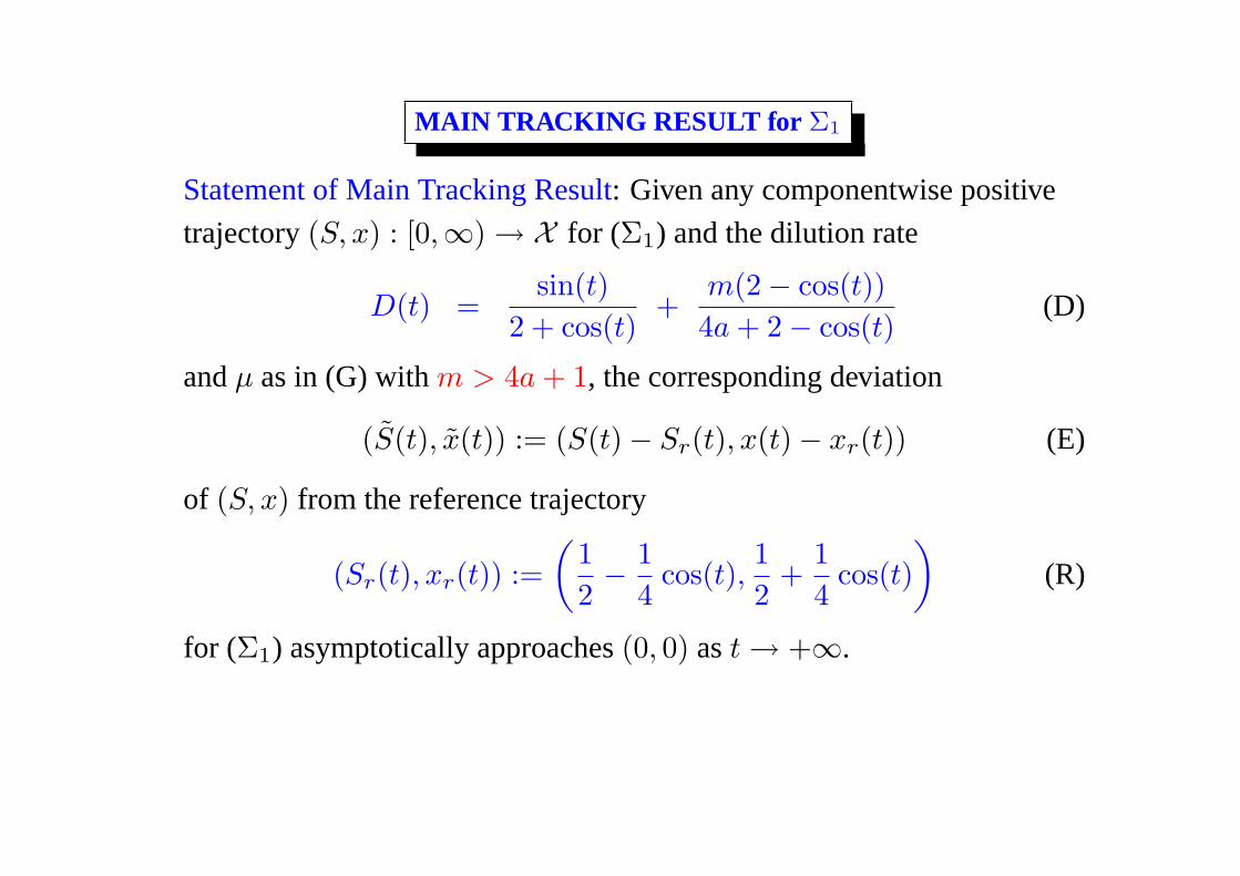
MAIN TRACKING RESULT for Σ1
Statement of Main Tracking Result: Given any componentwise positive
trajectory(S, x) : [0,∞) → X for (Σ1) and the dilution rate
D(t) =sin(t)
2 + cos(t)+
m(2− cos(t))4a + 2− cos(t)
(D)
andµ as in (G) withm > 4a + 1, the corresponding deviation
(S(t), x(t)) := (S(t)− Sr(t), x(t)− xr(t)) (E)
of (S, x) from the reference trajectory
(Sr(t), xr(t)) :=(
12− 1
4cos(t),
12
+14
cos(t))
(R)
for (Σ1) asymptotically approaches(0, 0) ast → +∞.

MAIN TRACKING RESULT for Σ1
Statement of Main Tracking Result: Given any componentwise positivetrajectory(S, x) : [0,∞) → X for (Σ1) and the dilution rate
D(t) =sin(t)
2 + cos(t)+
m(2− cos(t))4a + 2− cos(t)
(D)
andµ as in (G) withm > 4a + 1, the corresponding deviation
(S(t), x(t)) := (S(t)− Sr(t), x(t)− xr(t)) (E)
of (S, x) from the reference trajectory
(Sr(t), xr(t)) :=(
12− 1
4cos(t),
12
+14
cos(t))
(R)
for (Σ1) asymptotically approaches(0, 0) ast → +∞.
(Similar results hold if we instead pick anyxr(t) s.t.∃` > 0 s.t.∀t ≥ 0,max{`, |xr(t)|} ≤ xr(t) ≤ 3
4 andSr = 1− xr, for suitableD.)

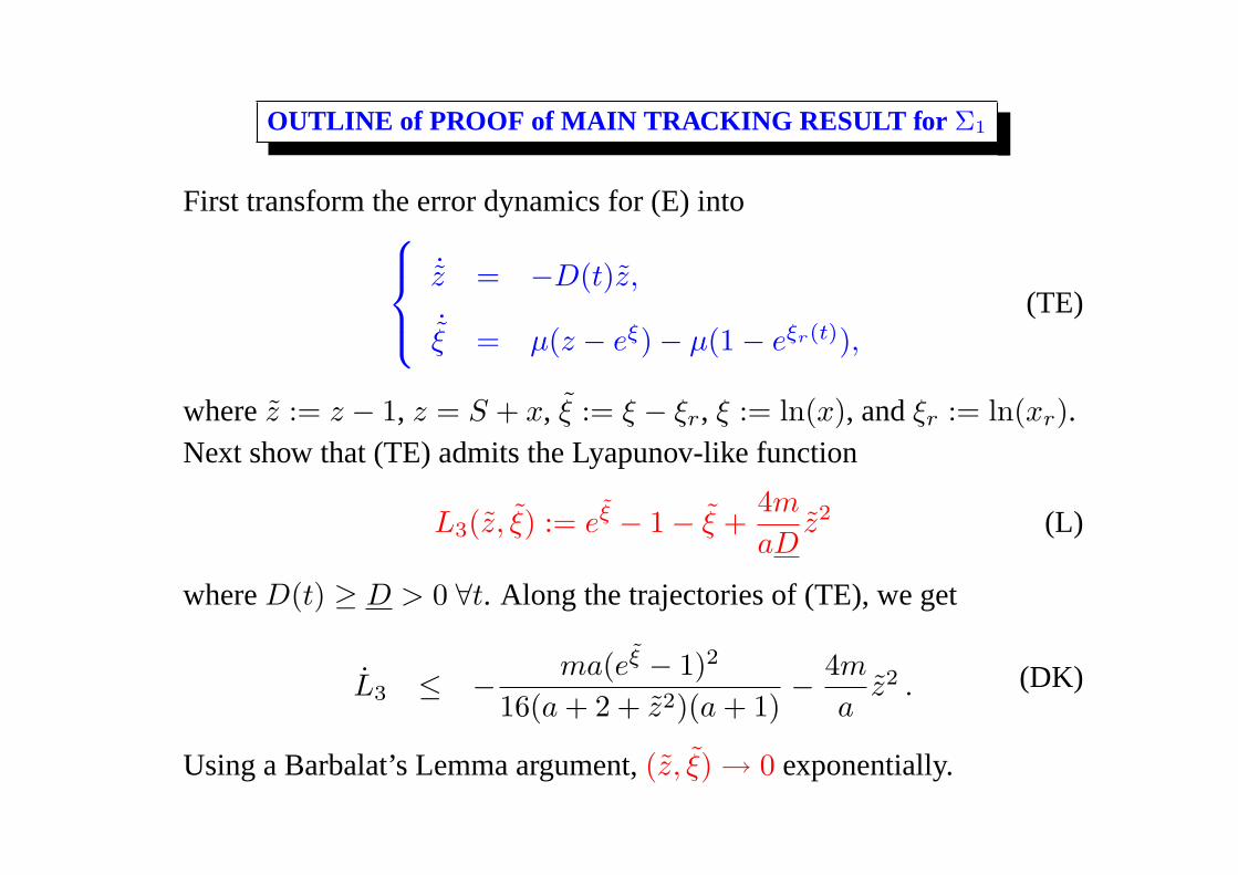
OUTLINE of PROOF of MAIN TRACKING RESULT for Σ1
First transform the error dynamics for (E) into
˙z = −D(t)z,
˙ξ = µ(z − eξ)− µ(1− eξr(t)),
(TE)
wherez := z − 1, z = S + x, ξ := ξ − ξr, ξ := ln(x), andξr := ln(xr).
OUTLINE of PROOF of MAIN TRACKING RESULT for Σ1
First transform the error dynamics for (E) into
˙z = −D(t)z,
˙ξ = µ(z − eξ)− µ(1− eξr(t)),
(TE)
wherez := z − 1, z = S + x, ξ := ξ − ξr, ξ := ln(x), andξr := ln(xr).Next show that (TE) admits the Lyapunov-like function
L3(z, ξ) := eξ − 1− ξ +4m
aDz2 (L)
whereD(t) ≥ D > 0 ∀t. Along the trajectories of (TE), we get
L3 ≤ − ma(eξ − 1)2
16(a + 2 + z2)(a + 1)− 4m
az2 . (DK)
Using a Barbalat’s Lemma argument,(z, ξ) → 0 exponentially.
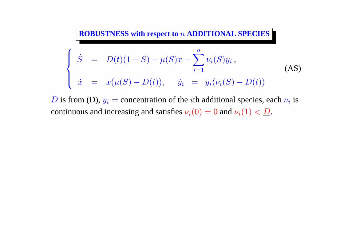
ROBUSTNESS with respect ton ADDITIONAL SPECIES
S = D(t)(1− S)− µ(S)x−n∑
i=1
νi(S)yi ,
x = x(µ(S)−D(t)), yi = yi(νi(S)−D(t))
(AS)
D is from (D),yi = concentration of theith additional species, eachνi is
continuous and increasing and satisfiesνi(0) = 0 andνi(1) < D.

ROBUSTNESS with respect ton ADDITIONAL SPECIES
S = D(t)(1− S)− µ(S)x−n∑
i=1
νi(S)yi ,
x = x(µ(S)−D(t)), yi = yi(νi(S)−D(t))
(AS)
D is from (D),yi = concentration of theith additional species, eachνi is
continuous and increasing and satisfiesνi(0) = 0 andνi(1) < D.
Multi-Species Result: The error between any componentwise
positive solution(S, x, y1, y2, . . . , yn) of (AS) and
(Sr, xr, 0, . . . , 0) =(
12− 1
4cos(t),
12
+14
cos(t), 0, . . . , 0)
converges exponentially to the zero vector ast → +∞.

ROBUSTNESS with respect ton ADDITIONAL SPECIES
S = D(t)(1− S)− µ(S)x−n∑
i=1
νi(S)yi ,
x = x(µ(S)−D(t)), yi = yi(νi(S)−D(t))
(AS)
D is from (D),yi = concentration of theith additional species, eachνi iscontinuous and increasing and satisfiesνi(0) = 0 andνi(1) < D.
Multi-Species Result: The error between any componentwisepositive solution(S, x, y1, y2, . . . , yn) of (AS) and
(Sr, xr, 0, . . . , 0) =(
12− 1
4cos(t),
12
+14
cos(t), 0, . . . , 0)
converges exponentially to the zero vector ast → +∞.
Significance:The stability of the reference trajectory (R) is robust withrespect to additional species that are exponentially decaying to extinction.

OUTLINE of PROOF of MULTI-SPECIES RESULT
Sinceνi(1) < D for eachi, the form of the dynamics forS along our
componentwise positive trajectories implies that there existε > 0 and
T ≥ 0 such that(i) S(t) ≤ 1 + ε for all t ≥ T and(ii) νi(1 + ε) < D for
all i = 1, 2, . . . , n. We next choose
δ := D − maxi=1,...,n
νi(1 + ε) > 0.

OUTLINE of PROOF of MULTI-SPECIES RESULT
Sinceνi(1) < D for eachi, the form of the dynamics forS along ourcomponentwise positive trajectories implies that there existε > 0 andT ≥ 0 such that(i) S(t) ≤ 1 + ε for all t ≥ T and(ii) νi(1 + ε) < D forall i = 1, 2, . . . , n. We next choose
δ := D − maxi=1,...,n
νi(1 + ε) > 0.
The result now follows using the Lyapunov-like function
L4(z, ξ, y1, ..., yn) = L3(z, ξ) + An∑
i=1
y2i , where A :=
16mn2
aδ.
in conjunction with Barbalat’s Lemma. Along the relevant trajectories,
L4 ≤ − ma(eξ − 1)2
16(a + 1)(a + 2 + z2)− 3m
az2 − 16mn2
a
n∑
i=1
y2i .
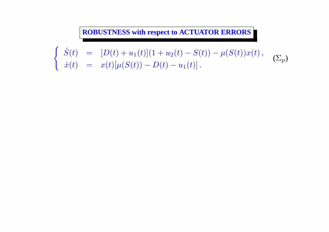
ROBUSTNESS with respect to ACTUATOR ERRORS
{S(t) = [D(t) + u1(t)](1 + u2(t)− S(t))− µ(S(t))x(t) ,
x(t) = x(t)[µ(S(t))−D(t)− u1(t)] .(Σp)
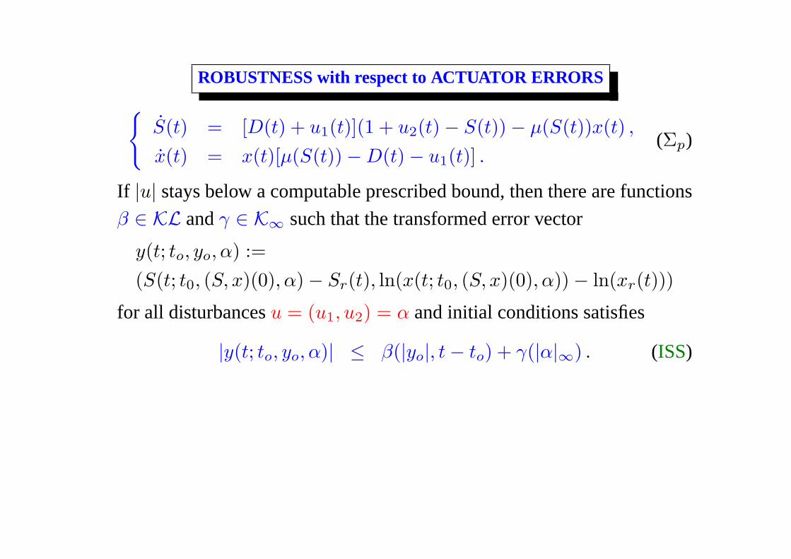
ROBUSTNESS with respect to ACTUATOR ERRORS
{S(t) = [D(t) + u1(t)](1 + u2(t)− S(t))− µ(S(t))x(t) ,
x(t) = x(t)[µ(S(t))−D(t)− u1(t)] .(Σp)
If |u| stays below a computable prescribed bound, then there are functions
β ∈ KL andγ ∈ K∞ such that the transformed error vector
y(t; to, yo, α) :=(S(t; t0, (S, x)(0), α)− Sr(t), ln(x(t; t0, (S, x)(0), α))− ln(xr(t)))
for all disturbancesu = (u1, u2) = α and initial conditions satisfies
|y(t; to, yo, α)| ≤ β(|yo|, t− to) + γ(|α|∞) . (ISS)
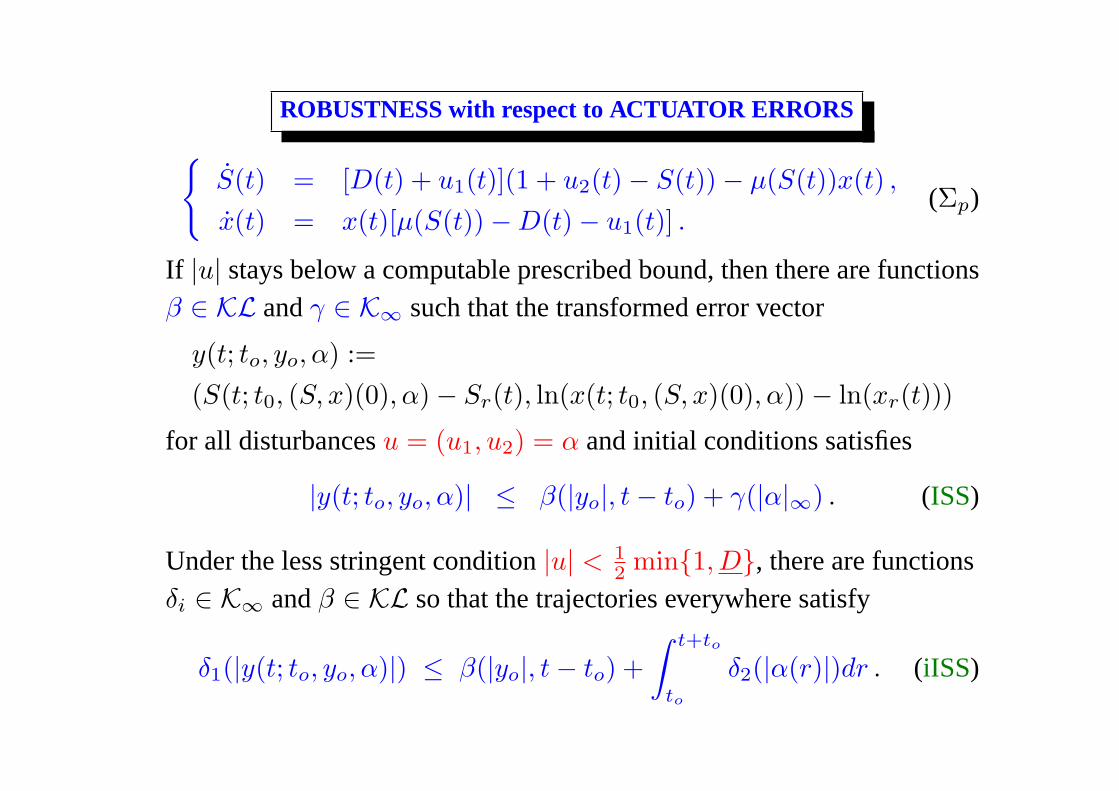
ROBUSTNESS with respect to ACTUATOR ERRORS
{S(t) = [D(t) + u1(t)](1 + u2(t)− S(t))− µ(S(t))x(t) ,
x(t) = x(t)[µ(S(t))−D(t)− u1(t)] .(Σp)
If |u| stays below a computable prescribed bound, then there are functionsβ ∈ KL andγ ∈ K∞ such that the transformed error vector
y(t; to, yo, α) :=(S(t; t0, (S, x)(0), α)− Sr(t), ln(x(t; t0, (S, x)(0), α))− ln(xr(t)))
for all disturbancesu = (u1, u2) = α and initial conditions satisfies
|y(t; to, yo, α)| ≤ β(|yo|, t− to) + γ(|α|∞) . (ISS)
Under the less stringent condition|u| < 12 min{1, D}, there are functions
δi ∈ K∞ andβ ∈ KL so that the trajectories everywhere satisfy
δ1(|y(t; to, yo, α)|) ≤ β(|yo|, t− to) +∫ t+to
to
δ2(|α(r)|)dr . (iISS)
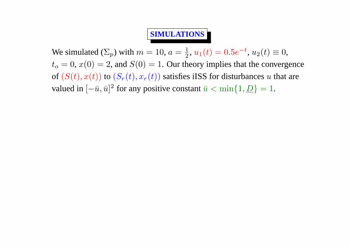
SIMULATIONS
We simulated (Σp) with m = 10, a = 12 , u1(t) = 0.5e−t, u2(t) ≡ 0,
to = 0, x(0) = 2, andS(0) = 1. Our theory implies that the convergence
of (S(t), x(t)) to (Sr(t), xr(t)) satisfies iISS for disturbancesu that are
valued in[−u, u]2 for any positive constantu < min{1, D} = 1.
SIMULATIONS
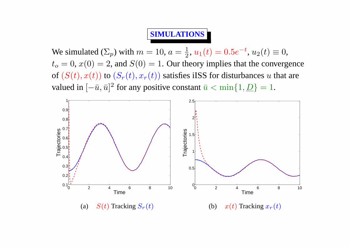
We simulated (Σp) with m = 10, a = 12 , u1(t) = 0.5e−t, u2(t) ≡ 0,
to = 0, x(0) = 2, andS(0) = 1. Our theory implies that the convergenceof (S(t), x(t)) to (Sr(t), xr(t)) satisfies iISS for disturbancesu that arevalued in[−u, u]2 for any positive constantu < min{1, D} = 1.
0 2 4 6 8 100.1
0.2
0.3
0.4
0.5
0.6
0.7
0.8
0.9
1
Time
Tra
ject
orie
s
(a) S(t) TrackingSr(t)
0 2 4 6 8 100
0.5
1
1.5
2
2.5
Time
Tra
ject
orie
s
(b) x(t) Trackingxr(t)

CONCLUSIONS
• Chemostats provide an important framework for modelingspecies
competingfor nutrients. They provide the foundation for much
current research inbioengineering, ecology, andpopulation biology.

CONCLUSIONS
• Chemostats provide an important framework for modelingspecies
competingfor nutrients. They provide the foundation for much
current research inbioengineering, ecology, andpopulation biology.
• For the case of one species competing for one nutrient and a suitable
time-varying dilution rate, we proved the stability of an appropriate
reference trajectoryusingLyapunov function methods.
• The stability is maintained when there are additional species that are
being driven to extinction, ordisturbances of small magnitudeon the
dilution rate and input nutrient concentration.
• Extensions to chemostats withmultiple competing species, time
delays, limited informationabout the current state, andmeasurement
uncertaintywould be desirable and are being studied.

ACKNOWLEDGEMENTS
• Malisoff was supported byNSF/DMS Grant 0424011. De Leenheer
was supported byNSF/DMS Grant 0500861. The authors thankJeff
SheldonandHairui Tu for assisting with the graphics.

ACKNOWLEDGEMENTS
• Malisoff was supported byNSF/DMS Grant 0424011. De Leenheer
was supported byNSF/DMS Grant 0500861. The authors thankJeff
SheldonandHairui Tu for assisting with the graphics.
• A journal version will appear inMathematical Biosciences and
Engineering. The authors thankYang Kuangfor the opportunity to
publish their work in his esteemed journal.
• Part of this work was done while Mazenc and De Leenheer visited
theLouisiana State University (LSU) Department of Mathematics.
They thank LSU for the kind hospitality they enjoyed.
• The authors thank the referees,Madalena Chaves, andEduardo
Sontagfor illuminating comments and discussions at the 45th IEEE
Conference on Decision and Control in San Diego, CA.