On the representation dimension of artin algebras.

Claus Michael Ringel

Abstract. The representation dimension of an artin algebra as introducedby M. Auslander in his Queen Mary Notes is the minimal possible global dimen-sion of the endomorphism ring of a generator-cogenerator. The following reportis based on two texts written in 2008 in connection with a workshop at Bielefeld.The first part presents a full proof that any torsionless-finite artin algebra hasrepresentation dimension at most 3, and provides a long list of classes of algebraswhich are torsionless-finite. In the second part we show that the representationdimension is adjusted very well to forming tensor products of algebras. In this wayone obtains a wealth of examples of artin algebras with large representation di-mension. In particular, we show: The tensor product of n representation-infinitepath algebras of bipartite quivers has representation dimension precisely n+ 2.

Let Λ be an artin algebra. The representation dimension repdimΛ of Λ was introduced1971 by M. Auslander in his Queen Mary Notes [A], it is the minimal possible globaldimension of the endomorphism ring of a generator-cogenerator (a generator-cogenerator

is a Λ-module M such that any indecomposable projective or injective Λ-module is adirect summand of M); a generator-cogenerator M such that the global dimension ofthe endomorphism ring of M is minimal will be said to be an Auslander generator. Allthe classes of algebras where Auslander was able to determine the precise representationdimension turned out to have representation dimension at most 3. Thus, he asked, onthe one hand, whether the representation dimension can be greater than 3, but also, onthe other hand, whether it always has to be finite. These questions have been answeredonly recently: The finiteness of the representation dimension was shown by Iyama [I1] in2003 (for a short proof using the notion of strongly quasi-hereditary algebras see [R4]).For some artin algebras Λ, one knows that repdimΛ ≤ LL(Λ) + 1, where LL(Λ) is theLoewy length of Λ. On the other hand, Rouquier [Rq] has shown that the representationdimension of the exterior algebra of a vector space of dimension n ≥ 1 is n+ 1.

The name representation dimension was coined by Auslander on the basis of his ob-servation that Λ is representation-finite if and only if repdimΛ ≤ 2. Not only Auslander,but later also many other mathematicians were able to prove that the representation di-mension of many well-known classes of artin algebras is bounded by 3. For artin algebraswith representation dimension at most 3, Igusa and Todorov [IT] have shown that thefinitistic dimension of these algebras is finite.

1

Our report is based on two texts written in 2008 in connection with a Bielefeld work-shop on the representation dimension [Bi].

Part I is a modified version of [R3] which was written as an introduction for the work-shop, it aimed at a general scheme for some of the known proofs for the upper bound 3,by providing the assertion 4.2 that any torsionless-finite artin algebra has representation

dimension at most 3. We recall that a Λ-module is said to be torsionless or divisible pro-vided it is a submodule of a projective module, or a factor module of an injective module,respectively. The artin algebra Λ is said to be torsionless-finite provided there are onlyfinitely many isomorphism classes of indecomposable torsionless Λ-modules. Two ingredi-ents are needed for the proof of 4.2, one is the characterization 4.3 of Auslander generatorswhich was used already by Auslander (at least implicitly) in the Queen Mary notes, thesecond is the bijection 3.2 between the isomorphism classes of the indecomposable tor-sionless and the indecomposable divisible modules which can be found in the appendix ofAuslander-Bridger [AB].

In Part II we want to outline that the representation dimension is adjusted verywell to forming tensor products of algebras. It should be stressed that already in 2000,Changchang Xi [X1] was drawing the attention to this relationship by showing that

repdimΛ⊗k Λ′ ≤ repdimΛ + repdimΛ′

for finite-dimensional k-algebras Λ,Λ′, provided k is a perfect field. In 2009, Oppermann[O1] gave a lattice criterion for obtaining a lower bound for the representation dimension(see 6.3) and we show (see 7.1) that this lattice construction is compatible with tensorproducts; this fact was also noted by Oppermann [O4]. In this way one obtains a wealth ofexamples with large representation dimension. These sections 6 and 7 are after-thoughtsto the workshop-lecture of Oppermann and a corresponding text was privately distributedafter the workshop. The last two sections show that sometimes one is able to determine theprecise value of the representation dimension. Namely, we will show in 9.4: Let Λ1, . . .Λn

be representation-infinite path algebras of bipartite quivers. Then the algebra Λ = Λ1 ⊗k

· · ·⊗kΛn has representation dimension precisely n+2. For quivers without multiple arrows,this result was presented at the Abel conference in Balestrand, June 2011, the exampleof the tensor product of two copies of the Kronecker algebra was exhibited already byOppermann at the Bielefeld workshop.

We consider an artin algebra Λ with duality functor D. Usually, we will consider leftΛ-modules of finite length and call them just modules.

Given a classM of modules, we denote by addM the modules which are (isomorphicto) direct summands of direct sums of modules inM. If M is a module, we write addM =addM. We say that M is finite provided there are only finitely many isomorphismclasses of indecomposable modules in addM, thus provided there exists a module M withaddM = addM.

Acknowledgment. The author is indebted to Dieter Happel and Steffen Oppermannfor remarks concerning the presentation of the paper.

2

Part I. Torsionless-finite artin algebras.

1. The torsionless modules for Λ and Λop

Let L = L(Λ) be the class of torsionless Λ-modules and P = P(Λ) the class ofprojective Λ-modules. Then P(Λ) ⊆ L(Λ), and we may consider the factor categoryL(Λ)/P(Λ) obtained from L(Λ) by factoring out the ideal of all maps which factor througha projective module.

(1.1) Theorem. There is a duality

η : L(Λ)/P(Λ) −→ L(Λop)/P(Λop)

with the following property: If U is a torsionless module, and f : P1(U) → P0(U) is a

projective presentation of U , then for η(U) we can take the image of Hom(f,Λ).

In the proof, we will use the following definition: We call an exact sequence P1 →P0 → P−1 with projective modules Pi strongly exact provided it remains exact when weapply Hom(−,Λ). Let E be the category of strongly exact sequences P1 → P0 → P−1 withprojective modules Pi (as a full subcategory of the category of complexes).

(1.2) Lemma. The exact sequence P1f−→ P0

g−→ P−1, with all Pi projective and

epi-mono factorization g = ue is strongly exact if and only if u is a left Λ-approximation.

Proof: Under the functor Hom(−,Λ), we obtain

Hom(P−1,Λ)g∗

−→ Hom(P0,Λ)f∗

−→ Hom(P1,Λ)

with zero composition. Assume that u is a left Λ-approximation. Given α ∈ Hom(P0,Λ)with f∗(α) = 0, we rewrite f∗(α) = αf. Now e is a cokernel of f , thus there is α′ withα = α′e. Since u is a left Λ-approximation, there is α′′ with α′ = α′′u. It follows thatα = α′e = α′′ue = α′′g = g∗(α′′).

Conversely, assume that the sequence (∗) is exact, let U be the image of g, thuse : P0 → U, u : U → P−1. Consider a map β : U → Λ. Then f∗(βe) = βef = 0, thus thereis β′ ∈ Hom(P−1,Λ) with g∗(β′) = βe. But g∗(β) = β′g = β′ue and βe = β′ue impliesβ = β′u, since e is an epimorphism.

Proof of Theorem 1.1. Let U be the full subcategory of E of all sequences whichare direct sums of sequences of the form

P −→ 0 −→ 0, P1−→ P −→ 0, 0 −→ P

1−→ P, 0 −→ 0 −→ P.

In order to define the functor q : E → L, let q(P1f−→ P0

g−→ P−1) be the image of g. Clearly,

q sends U onto P, thus it induces a functor

q : E/U −→ L/P.

3

Claim: This functor q is an equivalence.

First of all, the functor q is dense: starting with U ∈ L, let

P1f−→ P0

e−→ U −→ 0

be a projective presentation of U , let u : U → P−1 be a left Λ-approximation of U , andg = ue.

Second, the functor q is full. This follows from the lifting properties of projectivepresentations and left Λ-approximations.

It remains to show that q is faithful. We will give the proof in detail (and it maylook quite technical), however we should remark that all the arguments are standard; theyare the usual ones dealing with homotopy categories of complexes. Looking at strongly

exact sequences P1f−→ P0

g−→ P−1, one should observe that the image U of g has to be

considered as the essential information: starting from U , one may attach to it a projective

presentation (this means going from U to the left in order to obtain P1f−→ P0) as well as a

left Λ-approximation of U (this means going from U to the right in order to obtain P−1).

In order to show that q is faithful, let us consider the following commutative diagram

P1f

−−−−→ P0g

−−−−→ P−1

h1

y

h0

y

h−1

y

P ′1

f ′

−−−−→ P ′0

g′

−−−−→ P ′−1

with strongly exact rows. We consider epi-mono factorizations g = ue, g′ = u′e′ withe : P0 → U, u : U → P−1, e

′ : P ′0 → U ′, u′ : U ′ → P ′

−1, thus q(P•) = U, q(P ′•) = U ′. Assume

that q(h•) = ba, where a : U → X, b : X → U ′ with X projective. We have to show thath• belongs to U .

The factorizations g = ue, g′ = u′e′, q(h•) = ba provide the following equalities:

bae = e′h0, h−1u = u′ba.

Since u : U → P−1 is a left Λ-approximation and X is projective, there is a′ : P−1 → Xwith a′u = a. Since e′ : P ′

0 → U ′ is surjective and X is projective, there is b′ : X → P ′0

with e′b′ = b.

Finally, we need c : P0 → P ′1 with f ′c = h0 − b′ae. Write f ′ = v′w′ with w′ epi and v′

mono; in particular, v′ is the kernel of g′. Note that g′b′ae = u′e′b′ae = u′bae = u′e′h0 =g′h0, thus g′(h0 − b′ae) = g′h0 − g′b′ae = 0, thus h0 − b′ae factors through the kernel v′

of g′, say h0 − b′ae = v′c′. Since P0 is projective and w′ is surjective, we find c : P0 → P ′1

with w′c = c′, thus f ′c = v′w′c = v′c′ = h0 − b′ae.

4

Altogether, we obtain the following commutative diagram

P1f

−−−−→ P0g

−−−−→ P−1[

1

f

]

y

y

[

1

ae

]

y

[

a′

h−1−u′ba′

]

P1 ⊕ P0

[

0 0

1 0

]

−−−−→ P0 ⊕X

[

0 0

1 0

]

−−−−→ X ⊕ P ′−1

[

h1−cf c

]

y

y

[

h0−b′ae b′

]

y

[

u′b 1]

P ′1

f ′

−−−−→ P ′0

g′

−−−−→ P ′−1

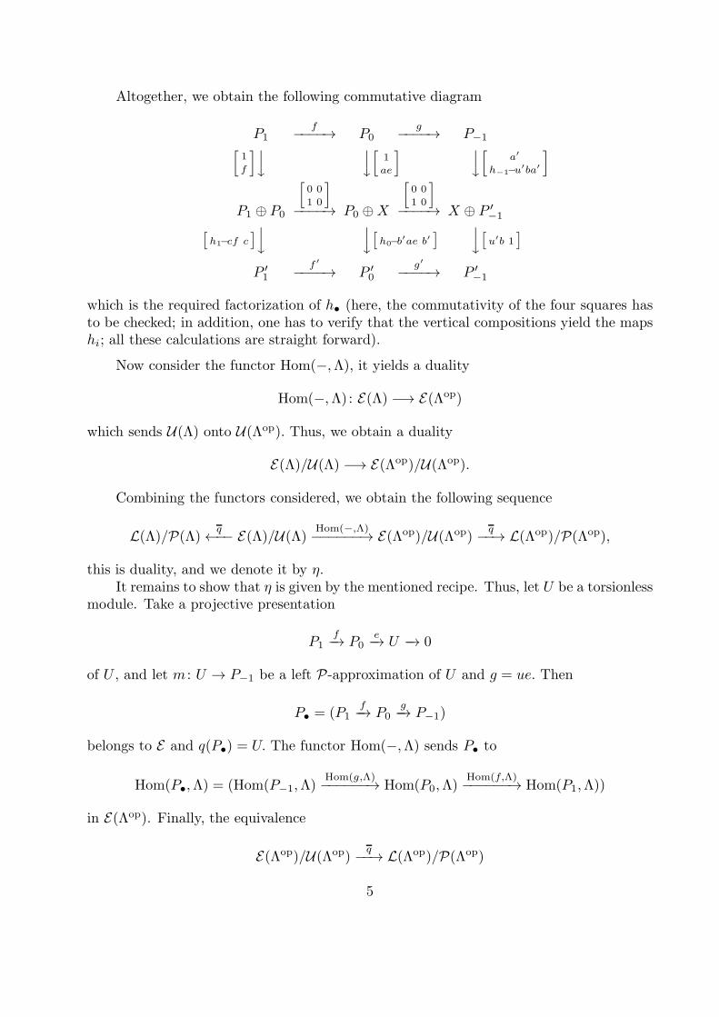
which is the required factorization of h• (here, the commutativity of the four squares hasto be checked; in addition, one has to verify that the vertical compositions yield the mapshi; all these calculations are straight forward).

Now consider the functor Hom(−,Λ), it yields a duality

Hom(−,Λ): E(Λ) −→ E(Λop)

which sends U(Λ) onto U(Λop). Thus, we obtain a duality

E(Λ)/U(Λ) −→ E(Λop)/U(Λop).

Combining the functors considered, we obtain the following sequence

L(Λ)/P(Λ)q←−− E(Λ)/U(Λ)

Hom(−,Λ)−−−−−−→ E(Λop)/U(Λop)

q−−→ L(Λop)/P(Λop),

this is duality, and we denote it by η.It remains to show that η is given by the mentioned recipe. Thus, let U be a torsionless

module. Take a projective presentation

P1f−→ P0

e−→ U −→ 0

of U , and let m : U → P−1 be a left P-approximation of U and g = ue. Then

P• = (P1f−→ P0

g−→ P−1)

belongs to E and q(P•) = U. The functor Hom(−,Λ) sends P• to

Hom(P•,Λ) = (Hom(P−1,Λ)Hom(g,Λ)−−−−−−→ Hom(P0,Λ)

Hom(f,Λ)−−−−−−→ Hom(P1,Λ))

in E(Λop). Finally, the equivalence

E(Λop)/U(Λop)q−−→ L(Λop)/P(Λop)

5

sends Hom(P•,Λ) to the image of Hom(f,Λ).

2. Consequences

(2.1) Corollary. There is a canonical bijection between the isomorphism classes of the

indecomposable torsionless Λ-modules and the isomorphism classes of the indecomposable

torsionless Λop-modules.

Proof: The functor Hom(−,Λ) provides a bijection between the isomorphism classes ofthe indecomposable projective Λ-modules and the isomorphism classes of the indecompos-able projective Λop-modules. For the non-projective indecomposable torsionless modules,we use the duality η given by Theorem 1.

Remark. As we have seen, there are canonical bijections between the indecomposableprojective Λ-modules and the indecomposable projective Λop-modules, as well betweenthe indecomposable non-projective torsionless Λ-modules and the indecomposable non-projective torsionless Λop-modules, both bijections being given by categorical dualities,but these bijections do not combine to a bijection with nice categorical properties. We willexhibit suitable examples below.

(2.2) Corollary. If Λ is torsionless-finite, also Λop is torsionless-finite.

Whereas corollaries 2.1 and 2.2 are of interest only for non-commutative artin algebras,the theorem itself is also of interest for Λ commutative.

(2.3) Corollary. For Λ a commutative artin algebra, the category L/P has a self-

duality.

For example, consider the factor algebra Λ = k[T ]/〈Tn〉 of the polynomial ring k[T ]in one variable, where k is a field. Since Λ is self-injective, all the modules are torsionless.Note that in this case, η coincides with the syzygy functor Ω.

3. The torsionless and the divisible Λ-modules

Let K = K(Λ) be the class of divisible Λ-modules. Of course, the duality functor Dprovides a bijection between the isomorphism classes of divisible modules and the isomor-phism classes of torsionless right modules.

We denote by Q = Q(Λ) the class of injective modules. Clearly, D provides a duality

D : L(Λop)/P(Λop) −→ K(Λ)/Q(Λ).

Thus, we can reformulate theorem 1 as follows: The categories L(Λ)/P(Λ) and K(Λ)/Q(Λ)are equivalent under the functor Dη. It seems to be worthwhile to replace the functor Dηby the functor Στ . Here, τ is the Auslander-Reiten translation and Σ is the suspensionfunctor (defined by Σ(V ) = I(V )/V, where I(V ) is an injective envelope of V ). Namely,

6

in order to calculate τ(U), we start with a minimal projective presentation f : P1 → P0

and take as τ(U) the kernel of

DHom(f,Λ): DHom(P1,Λ) −→ DHom(P0,Λ).

Now the kernel inclusion τ(U) ⊂ DHom(P1,Λ) is an injective envelope of τ(U); thusΣτ(U) is the image of DHom(f,Λ), but this image is Dη(U). Thus we see that Theorem1.1 can be formulated also as follows:

(3.1) Theorem. The categories L(Λ)/P(Λ) and K(Λ)/Q(Λ) are equivalent under

the functor γ = Στ .

(3.2) Corollary. If Λ is torsionless-finite, the number of isomorphism classes of

indecomposable divisible modules is equal to the number of isomorphism classes of inde-

composable torsionless modules.

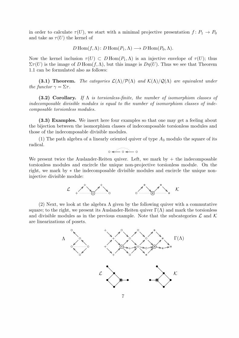
(3.3) Examples. We insert here four examples so that one may get a feeling aboutthe bijection between the isomorphism classes of indecomposable torsionless modules andthose of the indecomposable divisible modules.

(1) The path algebra of a linearly oriented quiver of type A3 modulo the square of itsradical.

................................................................... .........................................................................

.......

We present twice the Auslander-Reiten quiver. Left, we mark by + the indecomposabletorsionless modules and encircle the unique non-projective torsionless module. On theright, we mark by ∗ the indecomposable divisible modules and encircle the unique non-injective divisible module:

+

+

+

+

...........................................................

............................................................. ................................................. ........

................................................................. ................................................. ........

....

......... .........L

∗

∗

∗

∗...........................................................

............................................................. ................................................. ........

................................................................. ................................................. ........

....

......... .........K

(2) Next, we look at the algebra Λ given by the following quiver with a commutativesquare; to the right, we present its Auslander-Reiten quiver Γ(Λ) and mark the torsionlessand divisible modules as in the previous example. Note that the subcategories L and Kare linearizations of posets.

.............................................................

..................

..................

.........................

..................

..................

.....................................................................

.................

..................

..................

.........................

. . . . . . . . .

Λ

+

+

+

+

+ +

∗

∗

∗

∗

∗

∗........................................................... .......

....................................................

.............................................................

.............................................................

.............................................................

.............................................................

.............................................................

.............................................................

.............................................................

.............................................................

.............................................................

.............................................................................................................. ........

....

................................................. ............

................................................. ............

................................................. ............

................................................. ............

................................................. ............

................................................. ............

................................................. ............

................................................. ............

................................................. ............

................................................. ............

....................................... ............ ....................................... ............ ....................................... ................................................... ............

....................................... ............

....................................... ............

Γ(Λ)

•

•

•

•

• •.....................................................................

..................

..................................................................

...........................................................................................................................................................................................

L

• •

•

•

•

•..............................................................................

..................

..........

...............................................

......................................................................................................................................... ..................................................

K

7

(3) The local algebra Λ with generators x, y and relations x2 = y2 and yx = 0. Inorder to present Λ-modules, we use here the following convention: the bullets represent basevectors, the lines marked by x or y show that the multiplication by x or y, respectively,sends the upper base vector to the lower one (all other multiplications by x or y aresupposed to be zero). The upper line shows all the indecomposable modules in L, thelower one those in K.

•

• •

• •

........................................................................................................................................................................................................................................................................................

x

x

y

yx

ΛΛ

• •

•

•........................................................................................................

x y•

•

....................................................x

• •

• •................................................................................................................

............................................

xx

y

•

• •

•

•

........................................................................................................................................................................................................................................

................................................

y

y

x

x

yΛDΛ •

•

•........................................................................................................

x y • •

•

....................................................

y

•

•

•

•

................................................................................................................

............................................

y xy

L

K

Let us stress the following: All the indecomposable modules in L \ P as well as those inK \ Q are Λ′-modules, where Λ′ = k[x, y]/〈x, y〉2. Note that the category of Λ′-modules isstably equivalent to the category of Kronecker modules, thus all its regular components arehomogeneous tubes. In L we find two indecomposable modules which belong to one tube,in K we find two indecomposable modules which belong to another tube. The algebra Λ′

has an automorphism which exchanges these two tubes; this is an outer automorphism,and it cannot be lifted to an automorphism of Λ itself.

(4) In the last example to be presented here, L (and therefore also K) will be infinite.We consider the quiver

.....................................................................................

................................................................................... ............

................................................................................... ............

................................................................................... ............

................................................................................... ............

.....................................................................................

1

2 3

4

α

β

β′

β

β′

α

with the relations αβ = βα and αβ′ = β′α, thus we deal with the tensor product Λ ofthe Kronecker algebra and the path algebra of the quiver of type A2 (note that tensorproducts of algebras will be discussed in the second part of this paper in more detail).For any vertex i, we denote by S(i), P (i), Q(i) the simple, or indecomposable projectiveor indecomposable injective Λ-module corresponding to i, respectively.

The categories L and K can be described very well using the category of Kroneckermodules. By definition, the Kronecker quiver K has two vertices, a source and a sink, andtwo arrows going from the source to the sink. Thus a Kronecker module is a quadruple(U, V, w, w′) consisting of two vector spaces U, V and two linear maps w,w′ : U → V . We

8

define functors η, η′ : mod kK → modΛ, sending M = (U, V, w, w′) to the representations

.................................................................................................

........................................................................................... ............

................................................................................................. ............

........................................................................................... ............

................................................................................................. ............

.................................................................................................

0

V U

V ⊕ V

[

1

0

]

[

0

1

]

[ w

w′

]

η(M) =

.................................................................................................

........................................................................................... ............

..................................................................................... ............

........................................................................................... ............

................................................................................................. ............

.................................................................................................

U ⊕ U

V U

0

[ 1 0 ]

[ 0 1 ][w w′ ]

η′(M) =

these functors η, η′ are full embeddings.Let us denote by I the indecomposable injective Kronecker module of length 3, by T

the indecomposable projective Kronecker module of length 3, then clearly

η(I) = radP (1) and η′(T ) = Q(4)/ soc,

and the dimension vector of η(I) is0

1 22 , that of η′(T ) is

22 10 . If M is an indecomposable

Kronecker module, then either M is simple injective and η(M) = S(3), or else M iscogenerated by I, and η(M) is cogenerated by radP (1), thus η(M) is a torsionless Λ-module. Similarly, either M is simple projective and η′(M) = S(2), or else M is generatedby T and η′(M) is generated by Q(4)/ soc, so that η′(M) is divisible.

On the other hand, nearly all indecomposable torsionless Λ-modules are in the im-age of the functor η, the only exceptions are the indecomposable projective modulesP (1), P (3), P (4). Similarly, nearly all indecomposable divisible Λ-modules are in theimage of the functor η′, the only exceptions are the indecomposable injective modulesQ(1), Q(2), Q(4).

Altogether, one sees that the category L has the following Auslander-Reiten quiver

P (4)

P (2)

P (3)

P (1)

02 14

03 26

04 83

03 46

02 34

01 22

...................................................................

...................................................................

....................................................... ............

....................................................... ............

....................................................... ............

...................................................................

...................................................................

................................................................... ....................................................... ........

....

....................................................... ............

............................................ .........

................................................................................... ....................................................... ........

....

....................................................... ............

...................................................................

...................................................................

...................................................................

tubes

...........................................................................................................................................................................................................................................................................................................................................................................................................................................................

.....................................................................

...........................................................................................

........................................................

..................................

.

....

.

.

.

.

.

.

.

.

.

.

.

.

.

.

.

.

.

.

.

.

.

.

.

.

.

.

.

.

.

.

.

.

.

.

.

.

.

.

.

.

.

.

.

.

.

.

.

.

.

.

.

.

.

.

.

.

.

.

.

.

.

.

.

.

.

.

.

.

.

.

.

.

.

.

.

.

.

.

.

.

.

.

.

.

.

.

.

.

.

.

.

.

.

.

.

.

.

.

.

.

.

.

.

.

.

.

.

.

.

.

.

.

.

.

.

.

.

.

.

.

.

.

.

.

.

.

.

.

.

.

.

.

.

.

.

.

.

.

.

.

.

.

.

.

.

.

.

.

.

.

.

.

.

.

.

.

.

.

.

.

.

.

.

.

.

.

.

.

.

.

.

.

.

.

.

.

.

.

.

.

.

.

.

.

.

.

.

.

.

.

.

.

.

.

.

.

.

.

.

.

.

.

.

.

.

.

.

.

.

.

.

.

.

.

.

.

.

.

.

.

.

.

.

.

.

.

.

.

.

.

.

.

.

.

.

.

.

.

.

.

.

.

.

.

.

.

.

.

.

.

.

.

.

.

.

.

.

.

.

.

.

.

.

.

.

.

.

.

.

.

.

.

.

.

.

.

.

.

.

.

.

.

.

.

.

.

.

.

.

.

.

.

.

.

.

.

.

.

.

.

.

.

.

.

.

.

.

.

.

.

.

.

.

.

.

.

.

.

.

.

.

.

.

.

.

.

.

.

.

.

.

.

.

.

.

.

.

.

.

.

.

.

.

.

.

.

.

.

.

.

.

.

.

.

.

.

.

.

.

.

.

.

.

.

.

.

.

.

.

.

.

.

.

.

.

.

.

.

.

.

.

.

.

.

.

.

.

.

.

.

.

.

.

.

.

.

.

.

.

.

.

.

.

.

.

.

.

.

.

.

.

.

.

.

.

.

.

.

.

.

.

.

.

.

.

.

.

.

.

.

.

.

.

.

.

.

.

.

.

.

.

.

.

.

.

.

.

.

.

.

.

.

.

.

.

.

.

.

.

.

.

.

.

.

.

.

.

.

.

.

.

.

.

.

.

.

.

.

.

.

.

.

.

.

.

.

.

.

.

.

.

.

.

.

.

.

.

.

.

.

.

.

.

.

.

.

.

.

.

.

.

.

.

.

.

.

.

.

.

.

.

.

.

.

.

.

.

.

.

.

.

.

.

.

.

.

.

.

.

.

.

.

.

.

.

.

.

.

.

.

.

.

.

.

.

.

.

.

.

.

.

.

.

.

.

.

.

.

.

.

.

.

.

.

.

.

.

.

.

.

.

.

.

.

.

.

.

.

.

.

.

.

.

.

.

.

.

.

.

.

.

.

.

.

.

.

.

.

.

.

.

.

.

.

.

.

.

.

.

.

.

.

.

.

.

.

.

.

.

.

.

.

.

.

.

.

.

.

.

.

.

.

.

.

.

.

.

.

.

.

.

.

.

.

.

.

.

.

.

.

.

.

.

.

.

.

.

.

.

.

.

.

.

.

.

.

.

.

.

.

.

.

.

.

.

.

.

.

.

.

.

.

.

.

.

.

.

.

.

.

.

.

.

.

.

.

.

.

.

.

.

.

.

.

.

.

.

.

.

.

.

.

.

.

.

.

.

.

.

.

.

.

.

.

.

.

.

.

.

.

.

.

.

.

.

.

.

.

.

.

.

.

.

.

.

.

.

.

.

.

.

.

.

.

.

.

.

.

.

.

.

.

.

.

.

.

.

.

.

.

.

.

.

.

.

.

.

.

.

.

.

.

.

.

.

.

.

.

.

.

.

.

.

.

.

.

.

.

.

.

.

.

.

.

.

.

.

.

.

.

.

.

.

.

.

.

.

.

.

.

.

.

.

.

.

.

.

.

.

.

.

.

.

.

.

.

.

.

.

.

.

.

.

.

.

.

.

.

.

.

.

.

.

.

.

.

.

.

.

.

.

.

.

.

.

.

.

.

.

.

.

.

.

.

.

.

.

.

.

.

.

.

.

.

.

.

.

.

.

.

.

.

.

.

.

.

.

.

.

.

.

.

.

.

.

.

.

.

.

.

.

.

.

.

.

.

.

.

.

.

.

.

.

.

.

.

.

.

.

.

.

.

.

.

.

.

.

.

.

.

.

.

.

.

.

.

.

.

.

.

.

.

.

.

.

.

.

.

.

.

.

.

.

.

.

.

.

.

.

.

.

.

.

.

.

.

.

.

.

.

.

.

.

.

.

.

.

.

.

.

.

.

.

.

.

.

.

.

.

.

.

.

.

.

.

.

.

.

.

.

.

.

.

.

.

.

.

.

.

.

.

.

.

.

.

.

.

.

.

.

.

.

.

.

.

.

.

.

.

.

.

.

.

.

.

.

.

.

.

.

.

.

.

.

.

.

.

.

.

.

.

.

.

.

.

.

.

.

.

.

.

.

.

.

.

.

.

.

.

.

.

.

.

.

.

.

.

.

.

.

.

.

.

.

.

.

.

.

.

.

.

.

.

.

.

.

.

.

.

.

.

.

.

.

.

.

.

.

.

.

.

.

.

.

.

.

.

.

.

.

.

.

.

.

.

.

.

.

.

.

.

.

.

.

.

.

.

.

.

.

.

.

.

.

.

.

.

.

.

.

.

.

.

.

.

.

.

.

.

.

.

.

.

.

.

.

.

.

.

.

.

.

.

.

.

.

.

.

.

.

.

.

.

.

.

.

.

.

.

.

.

.

.

.

.

.

.

.

.

.

.

.

.

.

.

.

.

.

.

.

.

.

.

.

.

.

.

.

.

.

.

.

.

.

.

.

.

.

.

.

.

.

.

.

.

.

.

.

.

.

.

.

.

.

.

.

.

.

.

.

.

.

.

.

.

.

.

.

.

.

.

.

.

.

.

.

.

.

.

.

.

.

.

.

.

.

.

.

.

.

.

.

.

.

.

.

.

.

.

.

.

.

.

.

.

.

.

.

.

.

.

.

.

.

.

.

.

.

.

.

.

.

.

.

.

.

.

.

.

.

.

.

.

.

.

.

.

.

.

.

.

.

.

.

.

.

.

.

.

.

.

.

.

.

.

.

.

.

.

.

.

.

.

.

.

.

.

.

.

.

.

.

.

.

.

.

.

.

.

.

.

.

.

.

.

.

.

.

.

.

.

.

.

.

.

.

.

.

.

.

.

.

.

.

.

.

.

.

.

.

.

.

.

.

.

.

.

.

.

.

.

.

.

.

.

.

.

.

.

.

.

.

.

.

.

.

.

.

.

.

.

.

.

.

.

.

.

.

.

.

.

.

.

.

.

.

.

.

.

.

.

.

.

.

.

.

.

.

.

.

.

.

.

.

.

.

.

.

.

.

.

.

.

.

.

.

.

.

.

.

.

.

.

.

.

.

.

.

.

.

.

.

.

.

.

.

.

.

.

.

.

.

.

.

.

.

.

.

.

.

.

.

.

.

.

.

.

.

.

.

.

.

.

.

.

.

.

.

.

.

.

.

.

.

.

.

.

.

.

.

.

.

.

.

.

.

.

.

.

.

.

.

.

.

.

.

.

.

.

.

.

.

.

.

.

.

.

.

.

.

.

.

.

.

.

.

.

.

.

.

.

.

.

.

.

.

.

.

.

.

.

.

.

.

.

.

.

.

.

.

.

.

.

.

.

.

.

.

.

.

.

.

.

.

.

.

.

.

.

.

.

.

.

.

.

.

.

.

.

.

.

.

.

.

.

.

.

.

.

.

.

.

.

.

.

.

.

.

.

.

.

.

.

.

.

.

.

.

.

.

.

.

.

.

.

.

.

.

.

.

.

.

.

.

.

.

.

.

.

.

.

.

.

.

.

.

.

.

.

.

.

.

.

.

.

.

.

.

.

.

.

.

.

.

.

.

.

.

.

.

.

.

.

.

.

.

.

.

.

.

.

.

.

.

.

.

.

.

.

.

.

.

.

.

.

.

.

.

.

.

.

.

.

.

.

.

.

.

.

.

.

.

.

.

.

.

.

.

.

.

.

.

.

.

.

.

.

.

.

.

.

.

.

.

.

.

.

.

.

.

.

.

.

.

.

.

.

.

.

.

.

.

.

.

.

.

.

.

.

.

.

.

.

.

.

.

.

.

.

.

.

.

.

.

.

.

.

.

.

.

.

.

.

.

.

.

.

.

.

.

.

.

.

.

.

.

.

.

.

.

.

.

.

.

.

.

.

.

.

.

.

.

.

.

.

.

.

.

.

.

.

.

.

.

.

.

.

.

.

.

.

.

.

.

.

.

.

.

.

.

.

.

.

.

.

.

.

.

.

.

.

.

.

.

.

.

.

.

.

.

.

.

.

.

.

.

.

.

.

.

.

.

.

.

.

.

.

.

.

.

.

.

.

.

.

.

.

.

.

.

.

.

.

.

.

.

.

.

.

.

.

.

.

.

.

.

.

.

.

.

.

.

.

.

.

.

.

.

.

.

.

.

.

.

.

.

.

.

.

.

.

.

.

.

.

.

.

.

.

.

.

.

.

.

.

.

.

.

.

.

.

.

.

.

.

.

.

.

.

.

.

.

.

.

.

.

.

.

.

.

.

.

.

.

.

.

.

.

.

.

.

.

.

.

.

.

.

.

.

.

.

.

.

.

.

.

.

.

.

.

.

.

.

.

.

.

.

.

.

.

.

.

.

.

.

.

.

.

.

.

.

.

.

.

.

.

.

.

.

.

.

.

.

.

.

.

.

.

.

.

.

.

.

.

.

.

.

.

.

.

.

.

.

.

.

.

.

.

.

.

.

.

.

.

.

.

.

.

.

.

.

.

.

.

.

.

.

.

.

.

.

.

.

.

.

.

.

.

.

.

.

.

.

.

.

.

.

.

.

.

.

.

.

.

.

.

.

.

.

.

.

.

.

.

.

.

.

.

.

.

.

.

.

.

.

.

.

.

.

.

.

.

.

.

.

.

.

.

.

.

.

.

.

.

.

.

.

.

.

.

.

.

.

.

.

.

.

.

.

.

.

.

.

.

.

.

.

.

.

.

.

.

.

.

.

.

.

.

.

.

.

.

.

.

.

.

.

.

.

.

.

.

.

.

.

.

.

.

.

.

.

.

.

.

.

.

.

.

.

.

.

.

.

.

.

.

.

.

.

.

.

.

.

.

.

.

.

.

.

.

.

.

.

.

.

.

.

.

.

.

.

.

.

.

.

.

.

.

.

.

.

.

.

.

.

.

.

.

.

.

.

.

.

.

.

.

.

.

.

.

.

.

.

.

.

.

.

.

.

.

.

.

.

.

.

.

.

.

.

.

.

.

.

.

.

.

.

.

.

.

.

.

.

.

.

.

.

.

.

.

.

.

.

.

.

.

.

.

.

.

.

.

.

.

.

.

.

.

.

.

.

.

.

.

.

.

.

.

.

.

.

.

.

.

.

.

.

.

.

.

.

.

.

.

.

.

.

.

.

.

.

.

.

.

.

.

.

.

.

.

.

.

.

.

.

.

.

.

.

.

.

.

.

.

.

.

.

.

.

.

.

.

.

.

.

.

.

.

.

.

.

.

.

.

.

.

.

.

.

.

.

.

.

.

.

.

.

.

.

.

.

.

.

.

.

.

.

.

.

.

.

.

.

.

.

.

.

.

.

.

.

.

.

.

.

.

.

.

.

.

.

.

.

.

.

.

.

.

.

.

.

.

.

.

.

.

.

.

.

.

.

.

.

.

.

.

.

.

.

.

.

.

.

.

.

.

.

.

.

.

.

.

.

.

.

.

.

.

.

.

.

.

.

.

.

.

.

.

.

.

.

.

.

.

.

.

.

.

.

.

.

.

.

.

.

.

.

.

.

.

.

.

.

.

.

.

.

.

.

.

.

.

.

.

.

.

.

.

.

.

.

.

.

.

.

.

.

.

.

.

.

.

.

.

.

.

.

.

.

.

.

.

.

.

.

.

.

.

.

.

.

.

.

.

.

.

.

.

.

.

.

.

.

.

.

.

.

.

.

.

.

.

.

.

.

.

.

.

.

.

.

.

.

.

.

.

.

.

.

.

.

.

.

.

.

.

.

.

.

.

.

.

.

.

.

.

.

.

.

.

.

.

.

.

.

.

.

.

.

.

.

.

.

.

.

.

.

.

.

.

.

.

.

.

.

.

.

.

.

.

.

.

.

.

.

.

.

.

.

.

.

.

.

.

.

.

.

.

.

.

.

.

.

.

.

.

.

.

.

.

.

.

.

.

.

.

.

.

.

.

.

.

.

.

.

.

.

.

.

.

.

.

.

.

.

.

.

.

.

.

.

.

.

.

.

.

.

.

.

.

.

.

.

.

.

.

.

.

.

.

.

.

.

.

.

.

.

.

.

.

.

......

where the dotted part are the torsionless modules which are in the image of the functorη. The category L/P is equivalent under η to the category of Kronecker modules withoutsimple direct summands.

Dually, the category K has the following Auslander-Reiten quiver:

Q(4)

Q(2)

Q(3)

Q(1)

22 10

43 20

64 80

83 40

62 30

41 20

...................................................................

...................................................................

................................................................... ....................................................... ........

....

....................................................... ............

............................................ ..........

.................................................................................. ....................................................... ........

....

....................................................... ............

...................................................................

................................................................... ....................................................... ........

....

....................................................... ............

...................................................................

...................................................................

................................................................... ....................................................... ........

....

tubes

...........................................................................................................................................................................................................................................................................................................................................................................................................................................................

.........................

...............................................

...........................................................................................

.............................................................................

.

.

.

.

.

.

.

.

.

.

.

.

.

.

.

.

.

.

.

.

.

.

.

.

.

.

.

.

.

.

.

.

.

.

.

.

.

.

.

.

.

.

.

.

.

.

.

.

.

.

.

.

.

.

.

.

.

.

.

.

.

.

.

.

.

.

.

.

.

.

.

.

.

.

.

.

.

.

.

.

.

.

.

.

.

.

.

.

.

.

.

.

.

.

.

.

.

.

.

.

.

.

.

.

.

.

.

.

.

.

.

.

.

.

.

.

.

.

.

.

.

.

.

.

.

.

.

.

.

.

.

.

.

.

.

.

.

.

.

.

.

.

.

.

.

.

.

.

.

.

.

.

.

.

.

.

.

.

.

.

.

.

.

.

.

.

.

.

.

.

.

.

.

.

.

.

.

.

.

.

.

.

.

.

.

.

.

.

.

.

.

.

.

.

.

.

.

.

.

.

.

.

.

.

.

.

.

.

.

.

.

.

.

.

.

.

.

.

.

.

.

.

.

.

.

.

.

.

.

.

.

.

.

.

.

.

.

.

.

.

.

.

.

.

.

.

.

.

.

.

.

.

.

.

.

.

.

.

.

.

.

.

.

.

.

.

.

.

.

.

.

.

.

.

.

.

.

.

.

.

.

.

.

.

.

.

.

.

.

.

.

.

.

.

.

.

.

.

.

.

.

.

.

.

.

.

.

.

.

.

.

.

.

.

.

.

.

.

.

.

.

.

.

.

.

.

.

.

.

.

.

.

.

.

.

.

.

.

.

.

.

.

.

.

.

.

.

.

.

.

.

.

.

.

.

.

.

.

.

.

.

.

.

.

.

.

.

.

.

.

.

.

.

.

.

.

.

.

.

.

.

.

.

.

.

.

.

.

.

.

.

.

.

.

.

.

.

.

.

.

.

.

.

.

.

.

.

.

.

.

.

.

.

.

.

.

.

.

.

.

.

.

.

.

.

.

.

.

.

.

.

.

.

.

.

.

.

.

.

.

.

.

.

.

.

.

.

.

.

.

.

.

.

.

.

.

.

.

.

.

.

.

.

.

.

.

.

.

.

.

.

.

.

.

.

.

.

.

.

.

.

.

.

.

.

.

.

.

.

.

.

.

.

.

.

.

.

.

.

.

.

.

.

.

.

.

.

.

.

.

.

.

.

.

.

.

.

.

.

.

.

.

.

.

.

.

.

.

.

.

.

.

.

.

.

.

.

.

.

.

.

.

.

.

.

.

.

.

.

.

.

.

.

.

.

.

.

.

.

.

.

.

.

.

.

.

.

.

.

.

.

.

.

.

.

.

.

.

.

.

.

.

.

.

.

.

.

.

.

.

.

.

.

.

.

.

.

.

.

.

.

.

.

.

.

.

.

.

.

.

.

.

.

.

.

.

.

.

.

.

.

.

.

.

.

.

.

.

.

.

.

.

.

.

.

.

.

.

.

.

.

.

.

.

.

.

.

.

.

.

.

.

.

.

.

.

.

.

.

.

.

.

.

.

.

.

.

.

.

.

.

.

.

.

.

.

.

.

.

.

.

.

.

.

.

.

.

.

.

.

.

.

.

.

.

.

.

.

.

.

.

.

.

.

.

.

.

.

.

.

.

.

.

.

.

.

.

.

.

.

.

.

.

.

.

.

.

.

.

.

.

.

.

.

.

.

.

.

.

.

.

.

.

.

.

.

.

.

.

.

.

.

.

.

.

.

.

.

.

.

.

.

.

.

.

.

.

.

.

.

.

.

.

.

.

.

.

.

.

.

.

.

.

.

.

.

.

.

.

.

.

.

.

.

.

.

.

.

.

.

.

.

.

.

.

.

.

.

.

.

.

.

.

.

.

.

.

.

.

.

.

.

.

.

.

.

.

.

.

.

.

.

.

.

.

.

.

.

.

.

.

.

.

.

.

.

.

.

.

.

.

.

.

.

.

.

.

.

.

.

.

.

.

.

.

.

.

.

.

.

.

.

.

.

.

.

.

.

.

.

.

.

.

.

.

.

.

.

.

.

.

.

.

.

.

.

.

.

.

.

.

.

.

.

.

.

.

.

.

.

.

.

.

.

.

.

.

.

.

.

.

.

.

.

.

.

.

.

.

.

.

.

.

.

.

.

.

.

.

.

.

.

.

.

.

.

.

.

.

.

.

.

.

.

.

.

.

.

.

.

.

.

.

.

.

.

.

.

.

.

.

.

.

.

.

.

.

.

.

.

.

.

.

.

.

.

.

.

.

.

.

.

.

.

.

.

.

.

.

.

.

.

.

.

.

.

.

.

.

.

.

.

.

.

.

.

.

.

.

.

.

.

.

.

.

.

.

.

.

.

.

.

.

.

.

.

.

.

.

.

.

.

.

.

.

.

.

.

.

.

.

.

.

.

.

.

.

.

.

.

.

.

.

.

.

.

.

.

.

.

.

.

.

.

.

.

.

.

.

.

.

.

.

.

.

.

.

.

.

.

.

.

.

.

.

.

.

.

.

.

.

.

.

.

.

.

.

.

.

.

.

.

.

.

.

.

.

.

.

.

.

.

.

.

.

.

.

.

.

.

.

.

.

.

.

.

.

.

.

.

.

.

.

.

.

.

.

.

.

.

.

.

.

.

.

.

.

.

.

.

.

.

.

.

.

.

.

.

.

.

.

.

.

.

.

.

.

.

.

.

.

.

.

.

.

.

.

.

.

.

.

.

.

.

.

.

.

.

.

.

.

.

.

.

.

.

.

.

.

.

.

.

.

.

.

.

.

.

.

.

.

.

.

.

.

.

.

.

.

.

.

.

.

.

.

.

.

.

.

.

.

.

.

.

.

.

.

.

.

.

.

.

.

.

.

.

.

.

.

.

.

.

.

.

.

.

.

.

.

.

.

.

.

.

.

.

.

.

.

.

.

.

.

.

.

.

.

.

.

.

.

.

.

.

.

.

.

.

.

.

.

.

.

.

.

.

.

.

.

.

.

.

.

.

.

.

.

.

.

.

.

.

.

.

.

.

.

.

.

.

.

.

.

.

.

.

.

.

.

.

.

.

.

.

.

.

.

.

.

.

.

.

.

.

.

.

.

.

.

.

.

.

.

.

.

.

.

.

.

.

.

.

.

.

.

.

.

.

.

.

.

.

.

.

.

.

.

.

.

.

.

.

.

.

.

.

.

.

.

.

.

.

.

.

.

.

.

.

.

.

.

.

.

.

.

.

.

.

.

.

.

.

.

.

.

.

.

.

.

.

.

.

.

.

.

.

.

.

.

.

.

.

.

.

.

.

.

.

.

.

.

.

.

.

.

.

.

.

.

.

.

.

.

.

.

.

.

.

.

.

.

.

.

.

.

.

.

.

.

.

.

.

.

.

.

.

.

.

.

.

.

.

.

.

.

.

.

.

.

.

.

.

.

.

.

.

.

.

.

.

.

.

.

.

.

.

.

.

.

.

.

.

.

.

.

.

.

.

.

.

.

.

.

.

.

.

.

.

.

.

.

.

.

.

.

.

.

.

.

.

.

.

.

.

.

.

.

.

.

.

.

.

.

.

.

.

.

.

.

.

.

.

.

.

.

.

.

.

.

.

.

.

.

.

.

.

.

.

.

.

.

.

.

.

.

.

.

.

.

.

.

.

.

.

.

.

.

.

.

.

.

.

.

.

.

.

.

.

.

.

.

.

.

.

.

.

.

.

.

.

.

.

.

.

.

.

.

.

.

.

.

.

.

.

.

.

.

.

.

.

.

.

.

.

.

.

.

.

.

.

.

.

.

.

.

.

.

.

.

.

.

.

.

.

.

.

.

.

.

.

.

.

.

.

.

.

.

.

.

.

.

.

.

.

.

.

.

.

.

.

.

.

.

.

.

.

.

.

.

.

.

.

.

.

.

.

.

.

.

.

.

.

.

.

.

.

.

.

.

.

.

.

.

.

.

.

.

.

.

.

.

.

.

.

.

.

.

.

.

.

.

.

.

.

.

.

.

.

.

.

.

.

.

.

.

.

.

.

.

.

.

.

.

.

.

.

.

.

.

.

.

.

.

.

.

.

.

.

.

.

.

.

.

.

.

.

.

.

.

.

.

.

.

.

.

.

.

.

.

.

.

.

.

.

.

.

.

.

.

.

.

.

.

.

.

.

.

.

.

.

.

.

.

.

.

.

.

.

.

.

.

.

.

.

.

.

.

.

.

.

.

.

.

.

.

.

.

.

.

.

.

.

.

.

.

.

.

.

.

.

.

.

.

.

.

.

.

.

.

.

.

.

.

.

.

.

.

.

.

.

.

.

.

.

.

.

.

.

.

.

.

.

.

.

.

.

.

.

.

.

.

.

.

.

.

.

.

.

.

.

.

.

.

.

.

.

.

.

.

.

.

.

.

.

.

.

.

.

.

.

.

.

.

.

.

.

.

.

.

.

.

.

.

.

.

.

.

.

.

.

.

.

.

.

.

.

.

.

.

.

.

.

.

.

.

.

.

.

.

.

.

.

.

.

.

.

.

.

.

.

.

.

.

.

.

.

.

.

.

.

.

.

.

.

.

.

.

.

.

.

.

.

.

.

.

.

.

.

.

.

.

.

.

.

.

.

.

.

.

.

.

.

.

.

.

.

.

.

.

.

.

.

.

.

.

.

.

.

.

.

.

.

.

.

.

.

.

.

.

.

.

.

.

.

.

.

.

.

.

.

.

.

.

.

.

.

.

.

.

.

.

.

.

.

.

.

.

.

.

.

.

.

.

.

.

.

.

.

.

.

.

.

.

.

.

.

.

.

.

.

.

.

.

.

.

.

.

.

.

.

.

.

.

.

.

.

.

.

.

.

.

.

.

.

.

.

.

.

.

.

.

.

.

.

.

.

.

.

.

.

.

.

.

.

.

.

.

.

.

.

.

.

.

.

.

.

.

.

.

.

.

.

.

.

.

.

.

.

.

.

.

.

.

.

.

.

.

.

.

.

.

.

.

.

.

.

.

.

.

.

.

.

.

.

.

.

.

.

.

.

.

.

.

.

.

.

.

.

.

.

.

.

.

.

.

.

.

.

.

.

.

.

.

.

.

.

.

.

.

.

.

.

.

.

.

.

.

.

.

.

.

.

.

.

.

.

.

.

.

.

.

.

.

.

.

.

.

.

.

.

.

.

.

.

.

.

.

.

.

.

.

.

.

.

.

.

.

.

.

.

.

.

.

.

.

.

.

.

.

.

.

.

.

.

.

.

.

.

.

.

.

.

.

.

.

.

.

.

.

.

.

.

.

.

.

.

.

.

.

.

.

.

.

.

.

.

.

.

.

.

.

.

.

.

.

.

.

.

.

.

.

.

.

.

.

.

.

.

.

.

.

.

.

.

.

.

.

.

.

.

.

.

.

.

.

.

.

.

.

.

.

.

.

.

.

.

.

.

.

.

.

.

.

.

.

.

.

.

.

.

.

.

.

.

.

.

.

.

.

.

.

.

.

.

.

.

.

.

.

.

.

.

.

.

.

.

.

.

.

.

.

.

.

.

.

.

.

.

.

.

.

.

.

.

.

.

.

.

.

.

.

.

.

.

.

.

.

.

.

.

.

.

.

.

.

.

.

.

.

.

.

.

.

.

.

.

.

.

.

.

.

.

.

.

.

.

.

.

.

.

.

.

.

.

.

.

.

.

.

.

.

.

.

.

.

.

.

.

.

.

.

.

.

.

.

.

.

.

.

.

.

.

.

.

.

.

.

.

.

.

.

.

.

.

.

.

.

.

.

.

.

.

.

.

.

.

.

.

.

.

.

.

.

.

.

.

.

.

.

.

.

.

.

.

.

.

.

.

.

.

.

.

.

.

.

.

.

.

.

.

.

.

.

.

.

.

.

.

.

.

.

.

.

.

.

.

.

.

.

.

.

.

.

.

.

.

.

.

.

.

.

.

.

.

.

.

.

.

.

.

.

.

.

.

.

.

.

.

.

.

.

.

.

.

.

.

.

.

.

.

.

.

.

.

.

.

.

.

.

.

.

.

.

.

.

.

.

.

.

.

.

.

.

.

.

.

.

.

.

.

.

.

.

.

.

.

.

.

.

.

.

.

.

.

.

.

.

.

.

.

.

.

.

.

.

.

.

.

.

.

.

.

.

.

.

.

.

.

.

.

.

.

.

.

.

.

.

.

.

.

.

.

.

.

.

.

.

.

.

.

.

.

.

.

.

.

.

.

.

.

.

.

.

.

.

.

.

.

.

.

.

.

.

.

.

.

.

.

.

.

.

.

.

.

.

.

.

.

.

.

.

.

.

.

.

.

.

.

.

.

.

.

.

.

.

.

.

.

.

.

.

.

.

.

.

.

.

.

.

.

.

.

.

.

.

.

.

.

.

.

.

.

.

.

.

.

.

.

.

.

.

...

9

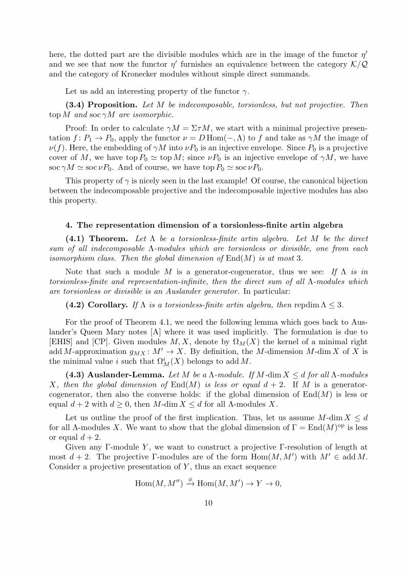
here, the dotted part are the divisible modules which are in the image of the functor η′

and we see that now the functor η′ furnishes an equivalence between the category K/Qand the category of Kronecker modules without simple direct summands.

Let us add an interesting property of the functor γ.

(3.4) Proposition. Let M be indecomposable, torsionless, but not projective. Then

topM and soc γM are isomorphic.

Proof: In order to calculate γM = ΣτM , we start with a minimal projective presen-tation f : P1 → P0, apply the functor ν = DHom(−,Λ) to f and take as γM the image ofν(f). Here, the embedding of γM into νP0 is an injective envelope. Since P0 is a projectivecover of M , we have topP0 ≃ topM ; since νP0 is an injective envelope of γM , we havesoc γM ≃ soc νP0. And of course, we have topP0 ≃ soc νP0.

This property of γ is nicely seen in the last example! Of course, the canonical bijectionbetween the indecomposable projective and the indecomposable injective modules has alsothis property.

4. The representation dimension of a torsionless-finite artin algebra

(4.1) Theorem. Let Λ be a torsionless-finite artin algebra. Let M be the direct

sum of all indecomposable Λ-modules which are torsionless or divisible, one from each

isomorphism class. Then the global dimension of End(M) is at most 3.

Note that such a module M is a generator-cogenerator, thus we see: If Λ is in

torsionless-finite and representation-infinite, then the direct sum of all Λ-modules which

are torsionless or divisible is an Auslander generator. In particular:

(4.2) Corollary. If Λ is a torsionless-finite artin algebra, then repdimΛ ≤ 3.

For the proof of Theorem 4.1, we need the following lemma which goes back to Aus-lander’s Queen Mary notes [A] where it was used implicitly. The formulation is due to[EHIS] and [CP]. Given modules M,X , denote by ΩM (X) the kernel of a minimal rightaddM -approximation gMX : M ′ → X . By definition, the M -dimension M -dimX of X isthe minimal value i such that Ωi

M (X) belongs to addM .

(4.3) Auslander-Lemma. Let M be a Λ-module. If M -dimX ≤ d for all Λ-modules

X, then the global dimension of End(M) is less or equal d + 2. If M is a generator-cogenerator, then also the converse holds: if the global dimension of End(M) is less orequal d+ 2 with d ≥ 0, then M -dimX ≤ d for all Λ-modules X .

Let us outline the proof of the first implication. Thus, let us assume M -dimX ≤ dfor all Λ-modules X . We want to show that the global dimension of Γ = End(M)op is lessor equal d+ 2.

Given any Γ-module Y , we want to construct a projective Γ-resolution of length atmost d + 2. The projective Γ-modules are of the form Hom(M,M ′) with M ′ ∈ addM.Consider a projective presentation of Y , thus an exact sequence

Hom(M,M ′′)φ−→ Hom(M,M ′)→ Y → 0,

10

with M ′,M ′′ ∈ addM . Note that φ = Hom(M, f) for some map f : M ′′ →M ′. Let X bethe kernel of f , thus Hom(M,X) is the kernel of Hom(M, f) = φ. Inductively, we constructminimal right addM -approximations

Migi−→ Ωi

M (X),

starting with Ω0M (X) = X , so that the kernel of gi is just Ωi+1

M , say with inclusion mapui+1 : Ω

i+1M →Mi. Thus, we get a sequence of maps

0→ ΩdM (X)

ud−→Md−1ud−1gd−1−−−−−−→Md−2 −→ · · · −→M1

u1g1−−−→M0

f0−→ X −→ 0

If we apply the functor Hom(M,−) to this sequence, we get an exact sequence

0→ Hom(M,ΩdM (X))→ Hom(M,Md−1)→ · · · → Hom(M,M0)→ Hom(M,X)→ 0

(here we use that we deal with right M -approximations and that Hom(M,−) is left exact).Since we assume that Ωd

M (X) is in addM , we see that we have constructed a projectiveresolution of Hom(M,X) of length d. Combining this with the exact sequence

0→ Hom(M,X)→ Hom(M,M ′′)φ−→ Hom(M,M ′)→ Y → 0,

we obtain a projective resolution of the Γ-module Y of length d + 2. This completes theproof that Γ, and therefore End(M) has global dimension at most d+ 2.

(4.4) Proof of Theorem 4.1. As before, let L be the class of torsionless Λ-modules,and K be the class of divisible Λ-modules. Since Λ is torsionless-finite there are Λ-modulesK,L with addK = K, and addL = L. Let M = K ⊕ L. We use the Auslander Lemma.

Let X be a Λ-module. Let U be the trace of K in X (this is the sum of the imagesof maps K → X). Since K is closed under direct sums and factor modules, U belongsto K (it is the largest submodule of X which belongs to K). Let p : V → X be a rightL-approximation of X (it exists, since we assume that L is finite). Since L contains all theprojective modules, it follows that p is surjective. Now we form the pullback

Vp

−−−−→ X

u′

x

x

u

W −−−−→p′

U

where u : U → X is the inclusion map. Since u is injective, also u′ is injective, thus W isa submodule of V ∈ L. Since L is closed under submodules, we see that W belongs to L.On the other hand, the pullback gives rise to the exact sequence

0 −→W

[

p′

−u′

]

−−−−−→ U ⊕ V[u p ]−−−−−→ X −→ 0

(the right exactness is due to the fact that p is surjective). By construction, the map[u p ] is a right M -approximation, thus ΩM (X) is a direct summand of W and thereforein L ⊆ addM. This completes the proof.

11

5. Classes of torsionless-finite artin algebras

In the following, let Λ be an artin algebra with radical J .

Before we deal with specific classes of torsionless-finite artin algebras, let us mentiontwo characterizations of torsionless-finite artin algebras:

(5.1) Proposition. An artin algebra Λ is torsionless-finite if and only if there exists

a faithful module M such that the subcategory of modules cogenerated by M is finite.

Proof. If Λ is torsionless-finite, we can take M = ΛΛ. Conversely, assume that Mis faithful and that the subcategory of modules cogenerated by M is finite. Since M isfaithful, the regular representation ΛΛ itself is cogenerated by M , thus all the torsionless-finite Λ-modules are cogenerated by M . This shows that Λ is torsionless-finite.

Actually, also non-faithful modules can similarly be used in order to characterizetorsionless-finiteness, for example we can take J (considered as a left Λ-module; note thatfor a non-zero artin algebra Λ, its radical J is never faithful, since it is annihilated by theright socle of Λ):

(5.2) Proposition. An artin algebra Λ is torsionless-finite if and only if the subcat-

egory of modules cogenerated by J is finite.

Proof: On the one hand, modules cogenerated by J are torsionless. Conversely, assumethat there are only finitely many isomorphism classes of indecomposable Λ-modules whichare cogenerated by J . Then Λ is torsionless-finite, according to following lemma.

(5.3) Lemma. Let N be an indecomposable torsionless Λ-module. Then either N is

projective or else N is cogenerated by J.

Proof: Let N be indecomposable and torsionless, but not cogenerated by J . We claimthat N is projective. Since N is torsionless, there is an inclusion map u : N → P =

⊕

Pi

with indecomposable projective modules Pi. Let πi : P → Pi be the canonical projectiononto the direct summand Pi of P and ǫi : Pi → Si the canonical projection of Pi onto itstop. If ǫπiu = 0 for all i, then N is contained in the radical of P , thus cogenerated by J ,a contradiction. Thus there is some index i with ǫπiu 6= 0, but this implies that πiu issurjective. Since this is a surjective map onto a projective module, we see that πiu is asplit epimorphism. But we assume that N is indecomposable, thus πiu is an isomorphism.This shows that N ≃ Pi is projective. Altogether, we see that there are only finitely manyisomorphism classes of indecomposable torsionless Λ-modules, namely those cogeneratedby J , as well as some additional ones which are projective.

Here are now some classes of torsionless-finite artin algebras:

(5.4) Artin algebras Λ with Λ/ soc(ΛΛ) representation-finite. Let N be anindecomposable torsionless Λ-module which is not projective. By Lemma 5.3, there is anembedding u : N → J t for some t. Let I = soc(ΛΛ). Then u(IN) = Iu(N) ⊆ I(J t) =0, thus IN = 0. This shows that N is a Λ/I-module. Thus N belongs to one of thefinitely many isomorphism classes of indecomposable Λ/I-modules. This shows that Λ istorsionless-finite.

12

If Jn = 0 and Λ/Jn−1 is representation-finite, then Λ is torsionless-finite. Namely,Jn−1 ⊆ soc(ΛΛ), thus, if Λ/J

n−1 is representation-finite, also its factor algebra Λ/ soc(ΛΛ)is torsionless-finite. This shows: If Jn = 0 and Λ/Jn−1 is representation-finite, then the

representation dimension of Λ is at most 3. (Auslander [A], Proposition, p.143)

(5.5) Artin algebras with radical square zero. Following Auslander (again [A],Proposition, p.143) This is the special case J2 = 0 of 5.4. Of course, here the proof of thetorsionless-finiteness is very easy: An indecomposable torsionless module is either projec-tive or simple. Similarly, an indecomposable divisible module is either injective or simple,and any simple module is either torsionless or divisible. Thus the module M exhibitedin Theorem 4.1 is the direct sum of all indecomposable projective, all indecomposableinjective, and all simple modules.

(5.6) Minimal representation-infinite algebras. Another special case of 5.4 isof interest: We say that Λ is minimal representation-infinite provided Λ is representation-infinite, but any proper factor algebra is representation-finite. If Λ is minimal representation-infinite, and n is minimal with Jn = 0, then Λ/Jn−1 is a proper factor algebra, thusrepresentation-finite.

(5.7) Hereditary artin algebras. If Λ is hereditary, then the only torsionlessmodules are the projective modules and the only divisible modules are the injective ones,thus the module M of Theorem 4.1 is the direct sum of all indecomposable modules whichare projective or injective. In this way, we recover Auslander’s result ([A], Proposition, p.147).

(5.8) Artin algebras stably equivalent to hereditary algebras. Let Λ be stablyequivalent to a hereditary artin algebra. Then an indecomposable torsionless moduleis either projective or simple ([AR1], Theorem 2.1), thus there are only finitely manyisomorphism classes of torsionless Λ-modules. Dually, an indecomposable divisible moduleis either injective or simple. Thus, again we see the structure of the module M of Theorem4.1 and we recover Proposition 4.7 of Auslander-Reiten [AR2].

(5.9) Right glued algebras (and similarly left glued algebras): An artin algebra Λ issaid to be right glued, provided the functor Hom(DΛ,−) is of finite length, or equivalently,provided almost all indecomposable modules have projective dimension equal to 1. Thecondition that Hom(DΛ,−) is of finite length implies that there are only finitely manyisomorphism classes of divisible Λ-modules. Also, the finiteness of the isomorphism classesof indecomposable modules of projective dimension greater than 1 implies torsionless-finiteness. We see that right glued algebras have representation dimension at most 3 (aresult of Coelho-Platzeck [CP]).

(5.10) Special biserial algebras without indecomposable projective-injectivemodules. In order to show that these artin algebras are torsionless-finite, we need thefollowing Lemma.

Lemma. Let Λ be special biserial and M a Λ-module. The following assertions are

equivalent.

(i) M is a direct sum of local string modules.

13

(ii) αM ∩ βM = 0 for arrows α 6= β.

Proof: (i) =⇒ (ii). We can assume that M is indecomposable, but then it is obviousthat condition (ii) is satisfied.

(ii) =⇒ (i): We can assume that M is indecomposable. For a band module, condition(ii) is clearly not satisfied. And for a string module M , condition (ii) is only satisfied incase M is local.

Proof that special biserial algebras without indecomposable projective-injective mod-ules are torsionless-finite: Assume that Λ is special biserial and that there is no indecom-posable projective-injective module. Then all the indecomposable projective modules arestring modules (and of course local). Thus any projective module satisfies the condition(i) and therefore also the condition (ii). But if a module M satisfies the condition (ii),also every submodule of M has this property. This shows that all torsionless modules sat-isfy the condition (ii). It follows that indecomposable torsionless modules are local stringmodules, and the number of such modules is finite.

It follows from 5.10 that all special biserial algebras have representation dimension at

most 3, as shown in [EHIS]. For the proof one uses the following general observation (dueto [EHIS] in case the representation dimension is 3):

(5.11) Proposition. Let Λ be an artin algebra. Let P be an indecomposable projective-

injective Λ-module. There is a minimal two-sided ideal I such that IP 6= 0. Let Λ′ = Λ/I.Then either Λ′ is semisimple or else repdimΛ ≤ repdimΛ′.

Proof: Note that all the indecomposable Λ-modules not isomorphic to P are annihi-lated by I, thus they are Λ′-modules.

First assume that Λ is representation finite, thus repdimΛ ≤ 2. Now Λ′ is also rep-resentation finite, and by assumption not semisimple, thus repdimΛ′ = 2. This yieldsthe claim. (Actually, Λ cannot be semisimple, since otherwise also Λ′ is semisimple, thusrepdimΛ = 2 and therefore repdimΛ = repdimΛ′.)

Now assume that Λ is not representation finite, with representation dimension d. LetM ′ be an Auslander generator for Λ′, thus, the second assertion of the Auslander-Lemmaasserts that M ′-dimX ≤ d for all Λ′-modules X . Let M = M ′ ⊕ P . This is clearlya generator-cogenerator. We want to show the any indecomposable Λ-module has M -dimension at most d (then End(M) has global dimension at most d and therefore therepresentation dimension of Λ is at most d).

Let X be an indecomposable Λ-module. Now X may be isomorphic to P , then X isin addM , thus its M -dimension is 0.

So let us assume that X is not isomorphic to P , thus a Λ′-module. Let g : M ′′ → Xbe a minimal right M ′-approximation of X . We claim that g is even a minimal right M -

approximation. Now M ′′ is in addM , thus we only have to show that any map f : Mi → Xfactors through g, where Mi is an indecomposable direct summand of M . This is clear incase Mi is a direct summand of M ′, thus we only have to look at the case Mi = P . Butsince X is annihilated by I, the map f : P → X vanishes on IP , thus f factors throughthe projection map p : P → P/IP , say f = f ′p with f ′ : P/IP → X. Since P/IP is an

14

indecomposable projective Λ′-module, it belongs to addM ′, thus f ′ factors through g, sayf ′ = gf ′′ for some f ′′ : P/IP → M ′′. Thus f = f ′p = gf ′′p factors through g. Thisconcludes the proof that g is a minimal right M -approximation.

Now ΩM (X) is the kernel of g, thus ΩM (X) = ΩM ′(X), in particular, this is againa Λ′-module. Thus, inductively we see that Ωi

M (X) = ΩiM ′(X) for all i. But we know

that ΩdM (X) = Ωd

M ′(X) is in addM ′, and addM ′ ⊆ addM . This shows that X hasM -dimension at most d.

There are many other classes of artin algebras studied in the literature which can beshown to be torsionless-finite, thus have representation dimension at most 3 (note that alsoTheorem 5.1 of [X1] deals with artin algebras which are divisible-finite, thus torsionless-finite).

(5.12) Further algebras with representation dimension 3. We have seen thatmany artin algebras of interest are torsionless-finite and thus their representation dimensionis at most 3. But we should note that not all artin algebras with representation dimensionat most 3 are torsionless-finite.

Namely, it is easy to construct special biserial algebras which are not torsionless-finite. And there are also many tilted algebras as well as canonical algebras which arenot torsionless-finite, whereas all tilted and all canonical algebras have representation-dimension at most 3, see Assem-Platzeck-Trepode [APT] and Oppermann [O3]. Actually,as Happel-Unger [HU] have shown, all piecewise hereditary algebras have representationdimension at most 3 (an algebra Λ is said to be piecewise hereditary provided the de-rived category Db(modΛ) is equivalent as a triangulated category to the bounded derivedcategory of some hereditary abelian category), but of course not all are torsionless-finite.

15

Part II. The Oppermann dimensionand tensor products of algebras.

We consider now k-algebras Λ, where k is a field.

6. Oppermann dimension.

(6.1) Let R = k[T1, . . . , Td] be the polynomial ring in d variables with coefficients ink and MaxR its maximal spectrum, this is the set of maximal ideals of R endowed withthe Zariski topology. For example, given α = (α1, . . . , αd) ∈ kd, there is the maximal idealmα = 〈Ti−αi | 1 ≤ i ≤ d〉. In case k is algebraically closed, we may identify in this way kd

with MaxR, otherwise kd yields only part of MaxR. In general, we will denote an elementof MaxR by α (or also by mα, if we want to stress that we consider α as a maximalideal), and Rα will denote the corresponding localization of R, whereas Sα = R/mα is thecorresponding simple R-module (note that all simple R-modules are obtained in this way).For any ring A, let finA be the category of finite length A-modules.

By definition, a Λ ⊗k R-lattice L is a finitely generated Λ ⊗k R-module which isprojective (thus free) as an R-module, we also will say that L is a d-dimensional lattice forΛ. Given a Λ⊗k R-lattice L, we may look at the functor

L⊗R − : finR −→ modΛ.

Since LR is projective, this is an exact functor. This means that given an exact sequenceof R-modules, applying L⊗R− we obtain an exact sequence of Λ-modules. Thus, if M,Nare R-modules, and d is a natural number, then looking at an element of ExtdR(M,N), wemay interpret this element as the equivalence class [ǫ] of a long exact sequence ǫ startingwith N and ending in M , and we may apply L ⊗R − to ǫ. We obtain in this way a longexact sequence L⊗R ǫ starting with L⊗R N and ending with L⊗R M and its equivalenceclass [L⊗R ǫ] in ExtdΛ(L⊗RM,L⊗RN). Since this equivalence class [L⊗R ǫ] only dependson [ǫ], we obtain the following function, also denoted by L⊗R −:

L⊗R − : ExtdR(M,N) −→ ExtdΛ(L⊗R M,L⊗R N), with (L⊗R −)[ǫ] = [L⊗R ǫ].

We say that L is a d-dimensional Oppermann lattice for Λ provided the set of α ∈MaxR such that

(L⊗R −)(

ExtdR(finRα, finRα))

6= 0,

is dense in MaxR; this means that for these α ∈ MaxR, there are modules M,N ∈ finRα

with(L⊗R −)

(

ExtdR(M,N))

6= 0.

Actually, instead of looking at all the modules in finRα, it is sufficient to deal with thesimple module Sα. One knows that the R-module ExtdR(Sα, Sα) is annihilated by mα andis one-dimensional as an R/mα-space; it is generated as an R/mα-space by the equivalenceclass of a long exact sequence of the form

ǫα : 0→ Sα →M1 → · · · →Md → Sα → 0

16

with Rα-modules Mi which are indecomposable and of length 2. If we tensor this exactsequence with L, we obtain an exact sequence

L⊗R ǫα : 0→ L⊗R Sα → L⊗R M1 → · · · → L⊗R Md → L⊗R Sα → 0

which yields an equivalence class [L ⊗R ǫα] in ExtdΛ(L ⊗R Sα, L ⊗R Sα). It is easy to seethat the following conditions are equivalent:

(i) (L⊗R −)(

ExtdR(finRα, finRα))

6= 0,

(ii) [L⊗R ǫα] 6= 0 as an element of ExtdΛ(L⊗R Sα, L⊗R Sα).

Thus we see: The d-dimensional lattice L is an Oppermann lattice for Λ provided the

set of α ∈ MaxR such that [L ⊗R ǫα] is a non-zero element of ExtdR(Sα, Sα) is dense in

MaxR.

By definition, the Oppermann dimension OdimΛ of Λ is the supremum of d such thatthere exists a d-dimensional Oppermann lattice L for Λ.

(6.2) Examples.(a) Let Λ be the path algebra of a representation-infinite quiver. Then OdimΛ = 1.(b) Let Λ be a representation-infinite k-algebra, where k is an algebraically closed field.

Then OdimΛ ≥ 1.

Proof. (a) The usual construction of one-parameter families of indecomposable Λ-modules for a representation-infinite quiver shows that OdimΛ ≥ 1. On the other hand,the path algebra of a quiver is hereditary, thus Ext2Λ = 0. This shows that the Oppermanndimension can be at most 1.

(b) This follows from the proof of the second Brauer-Thrall conjecture by Bautista[Bt] and [Bo], see also [Bo2] and [R5], [R6].

The following result of Oppermann ([O1], Corollary 3.8) shows that OdimΛ is alwaysfinite and that one obtains in this way an interesting lower bound for the representationdimension:

(6.3) Theorem (Oppermann). Let Λ be a finite-dimensional k-algebra which is

not semisimple. Then

OdimΛ + 2 ≤ repdimΛ.

One may ask whether one always has the equality OdimΛ + 2 = repdimΛ, thiscan be considered as a formidable extension of the assertion of the second Brauer-Thrallconjecture.

7. Tensor products of artin algebras.

Quite a long time ago, Changchang Xi [X1] has shown the following inequality: Givenfinite-dimensional k-algebras Λ,Λ′,

repdimΛ⊗k Λ′ ≤ repdimΛ + repdimΛ′,

17

provided k is a perfect field. This provides an upper bound for the representation dimensionof Λ⊗k Λ

′. But there is also a lower bound, which uses the Oppermann dimension. Let usdraw attention to the following fact:

(7.1) Theorem. Let Λ,Λ′ be finite-dimensional k-algebras. Let L be an Oppermann

lattice for Λ and L′ an Oppermann lattice for Λ′. Then L⊗k L′ is an Oppermann lattice

for Λ⊗k Λ′.

Proof: Theorem 7.1 is an immediate consequence of Theorem 3.1 in Chapter XI ofCartan-Eilenberg [CE].

Namely, let L be a d-dimensional Oppermann lattice for Λ and L′ a d′-dimensionalOppermann lattice for Λ′. Thus, L is an R-lattice with R = k[T1, . . . , Td] and say L′ is anR′-lattice, where R′ = k[T ′

1, . . . , T′d′ ] (with new variables T ′

i ). For α ∈ MaxR we choose an

exact sequence ǫα such that its equivalence class [ǫα] generates ExtdR(Sα, Sα); similarly, for

α′ ∈ MaxR′ we choose an exact sequence ǫα′ such that its equivalence class [ǫα′ ] generates

Extd′

R′(Sα′ , Sα′);Since L is an Oppermann lattice for Λ, the set of elements α ∈ MaxR such that

[L ⊗R ǫα] 6= 0 is dense in MaxR. Similarly, since L′ is an Oppermann lattice for Λ′, theset of elements α′ ∈ MaxR′ such that [L′ ⊗R′ ǫα′ ] 6= 0 is dense in MaxR′.

Now L⊗k L′ is a Λ⊗k Λ′ ⊗k R⊗k R′-lattice and we may look at

(L⊗k L′)⊗R⊗R′ (ǫα ∨ ǫα′).

We claim that its equivalence class is non-zero in Extd+d′

Λ⊗Λ′(L⊗L′⊗S(α,α′), L⊗L′⊗S(α,α′)).

This is a special case of Theorem XI.3.1 of Cartan-Eilenberg which asserts the following:Let Λ,Λ′ be left noetherian k-algebras, where k is a semisimple commutative ring. LetM be a finitely generated Λ-module and M ′ a finitely generated Λ′-module. Then thecanonical map

∨ : ExtdΛ(M,N)⊗k Extd′

Λ′(M ′, N ′) −→ Extd+d′

Λ⊗kΛ′(M ⊗k M ′, N ⊗k N ′)

is an isomorphism for any Λ-module N , Λ′-module N ′ and all d, d′ ∈ N.

It remains to note that for dense subsets X of MaxR and X ′ of MaxR′, the productX ×X ′ is of course dense in MaxR⊗k R′.

(7.2) Corollary. Let Λ,Λ′ be finite-dimensional k-algebras. Then

OdimΛ⊗k Λ′ ≥ OdimΛ + OdimΛ′.

Note that it is easy to provide examples where we have strict inequality: just takerepresentation-finite algebras Λ,Λ′ such that the Oppermann dimension of Λ ⊗k Λ′ is atleast 1, for example consider Λ = Λ′ = k[T ]/〈T 2〉, or take Λ,Λ′ path algebra of quivers oftype An with n ≥ 3. Note that the representation type of the tensor product of any twononsimple connected k-algebras with k an algebraically closed field, has been determinedby Leszczynski and A.Skowronski [LS].

18

The combination of the inequalities 6.3 and 7.2 yields:

(7.3) Corollary. Let Λ1, . . . ,Λn be finite-dimensional k-algebras. Then

repdimΛ1 ⊗k · · · ⊗k Λn ≥ 2 +∑n

i=1OdimΛi.

In particular, we see: Let Λ be the tensor product of n k-algebras with Oppermann

dimension greater or equal to 1. Then rep dimΛ ≥ n+ 2. Using 6.2, we see:

(7.4) Corollary.(a) If Λ is the tensor product of n path algebras of representation-infinite quivers, then

repdimΛ ≥ n+ 2.(b) If k is an algebraically closed field and Λ is the tensor product of n representation-

infinite k-algebras, then repdimΛ ≥ n+ 2.

As Happel has pointed out, the following remarkable consequence should be stressed:If Λ1,Λ2 are representation-infinite path algebras, then Λ1 ⊗ Λ2 is never a tilted algebra.After all, tilted algebras have representation dimension at most 3, whereas we have shownthat repdimΛ1 ⊗k Λ2 ≥ 4.

8. Nicely tiered algebras.

Let Q be a finite connected quiver. We say that Q is tiered with n+ 1 tiers providedthere is a surjective function l : Q0 → [0, n] = z ∈ Z | 0 ≤ z ≤ n such that for any arrowx → y one has l(x) = l(y) + 1. Such a function l, if it exists, is uniquely determined andis called the tier function for Q and l(x) is said to be the tier (or the tier number) of thevertex x. We say that Q is nicely tiered with n + 1 tiers provided Q is tiered with n + 1tiers, say with tier function l such that l(x) = 0 for all sinks x, and l(x) = n for all sourcesx. Clearly, Q is nicely tiered if and only if Q has no oriented cyclic paths and any maximalpath has length n. The tier function l of a nicely tiered quiver Q can be characterized asfollows: the tier number l(x) of a vertex x is the length of any maximal path starting in x.

Let Q be a nicely tiered quiver and M a representation of Q. We denote by M |[a, b]the restriction of M to the subquiver of all vertices x with a ≤ l(x) ≤ b. We say thata module lives in the interval [a, b] provided M = M |[a, b]. We say that a module M isgenerated in tier a provided its top lives in [a, a]. Dually, M is said to be cogenerated intier a provided its socle lives in [a, a]. Given a module M , and t ∈ N0, let tM be its t-thsocle (thus, there is the sequence of submodules

0 = 0M ⊆ 1M ⊆ · · · ⊆ tM ⊆M

such that tM/t−1M = soc(M/t−1M) for all t ≥ 1).

We say that an algebra is nicely tiered provided it is given by a nicely tiered quiverand a set of commutativity relations. Let Λ be nicely tiered. Then it follows: local sub-modules of projective modules are projective, colocal factor modules of injective modules

19

are injective. In particular: the socle of any projective module has support at some ofthe sinks, the top of any injective module has support at some of the sources. The Loewylength of a nicely tiered algebra with n + 1 tiers is precisely n + 1. Of special interest isthe following: For a nicely tiered algebra, any indecomposable module which is projective

or injective is solid (an indecomposable module over an artin algebra is said to be solid

provided its socle series coincides with its radical series).

(8.1) Proposition. Let Λ be nicely tiered algebra with n + 1 tiers. Assume that the

following conditions are satisfied for all indecomposable projective modules P, P ′ of Loewy

length at least 3:(P1) The module 2P is a brick (this means that any non-zero endomorphism is an auto-

morphism).(P2) If Hom(2P, 2P

′) 6= 0, then P can be embedded into P ′.

Let M be the direct sum of the modules tP with P indecomposable projective and t ≥ 2as well as the modules tQ with Q indecomposable injective, and t ≥ 1. Then End(M) hasglobal dimension at most n+ 2.

Remark. Note that the module M considered in 8.1 is both a generator and a cogener-ator, thus the number n+2 is an upper bound for the representation dimension of Λ. Herewe encounter again a class of algebras Λ where one now knows that repdimΛ ≤ LL(Λ)+1.

The proof of Proposition 8.1 follows the strategy of Iyama’s proof [I] of the finitenessof the representation dimension, as well as subsequent considerations by Oppermann [O1],Corollary A1 (but see already [A] as well as several joint papers with Dlab). It relies onthe following lemma shown in [R4]:

(8.2) Lemma. Let

∅ =M−1 ⊆M0 ⊆ · · · ⊆ Mn+1 =M

be finite sets of indecomposable Λ-modules. Let M be a Λ-module with addM = addMand Γ = End(M)op.

Assume that for any N ∈ Mi there is a monomorphism u : αN → N with αN ∈addMi−1 such that any radical map φ : N ′ → N with N ′ ∈ Mi factors through u.

Then the global dimension of Γ is at most n+ 2.

Let us outline the proof of 8.2. We consider the indecomposable projective Γ-modulesHom(M,N), where N is indecomposable in M. Assume that N belongs to Mi and nottoMi−1, for some i. Since N is not inMi−1, we see that u is a proper monomorphism.Let ∆(N) be the cokernel of Hom(M,u), thus we deal with the exact sequence

0→ Hom(M,αN)Hom(M,u)−−−−−−−→ Hom(M,N)→ ∆(N)→ 0.

We see that ∆(N) is the factor space of Hom(M,N) modulo those maps M → N whichfactor through u, thus through addMi−1.

The assumption that any radical map φ : N ′ → N with N ′ ∈ Mi factors throughu means the following: if we consider ∆(N) as a Γ-module, then it has one composition

20

factor of the form S(N) = topHom(M,N), all the other composition factors are of theform S(N ′) = topHom(M,N ′) with N ′ an indecomposable module inM which does notbelong toMi.

Since αN belongs to addMi−1, the projective Γ-module Hom(M,αN) is a direct sumof modules Hom(M,N ′) with N ′ inMi−1.

This shows that Γ is left strongly quasi-hereditary with n + 2 layers, thus has globaldimension at most n+ 2, according to [R4].

(8.3) Proof of 8.1. Let Λ be a nicely tiered algebra with n + 1 tiers such that theconditions (P1) and (P2) are satisfied.

The conditions (P1) and (P2) imply that corresponding properties are satisfied for tPwith t > 2.

(P1t) The module tP is a brick.(P2t) If Hom(tP, tP

′) 6= 0, then P can be embedded into P ′.

Proof: Let f : tP → tP′ be a non-zero homomorphism. Then also f |2P is non-zero,

since otherwise f would vanish at the tier 0, but the socle of P lives at the tier 0. Thus,any non-zero endomorphism of tP yields a non-zero endomorphism of 2P , by (P1) thisis an isomorphism; but if f |2P has zero kernel, the same is true for f : 2P → 2P ; thusf is a mono endomorphism, therefore an automorphism. This shows (P1t). Similarly, iff : tP → tP

′ is non-zero, then also f |2P is non-zero, therefore P can be embedded into P ′

by (P2).

We define sets of indecomposable modules Pi,Qi as follows:Let Pi be the set of modules tP , where P is indecomposable projective, t ≥ 2 and

LL(P )−t = i. The modules in Pi are indecomposable, according to condition (P1), see 8.1.The non-empty sets Pi are P0,P1, . . . ,Pn−1; the modules in P0 are the indecomposableprojective modules which are not simple, those in Pn−1 are the modules of the form 2Pwith P generated at tier n.

Let us collect some properties of the modules N in Pi. Such a module is generated attier g with 1 ≤ g ≤ n− i. (Namely, if P is indecomposable projective, then tP is of Loewylength t, thus generated at g = t − 1. Since t ≥ 2, we have g ≥ 1. Since P is of lengthl ≤ n + 1, we have t = l − i ≤ n + 1− i, thus g = t − 1 ≤ n − i.) The module N lives in[0, n− i] (since it is generated at tier g ≤ n− i), its socle lives at the vertices with tier 0,and the Loewy length of such a module N satisfies 2 ≤ LL(N) ≤ n− i+ 1.

Let Qi be the set of non-zero modules iQ with Q indecomposable injective and i ≤LL(Q). If Q is cogenerated at tier j, where 0 ≤ j ≤ n, then LL(Q) = n − j + 1, thus1 ≤ i ≤ n− j+1 implies that 0 ≤ j ≤ n− i+1. The non-empty sets Qi are Q1, . . . ,Qn+1.The modules in Q1 are just all the simple modules.

Since i ≥ 1, the module iQ is a non-zero submodule of Q, thus has simple socleand therefore is indecomposable. And again, we mention some additional properties for amodule N in Qi. It is generated at tier g with i − 1 ≤ g ≤ n, it lives in [i− 1, n] and itsLoewy length is precisely i.

Claim: If N is in Pi, then either radN belongs to Pi+1, or else radN is semisimple

and thus belongs to addQ1. If N in Qi with i ≥ 2, then radN belongs to Qi−1.

21

Proof: Let P be indecomposable projective of length l. If t = l − i ≥ 3, then N = tPbelongs to Pi and radN = t−1P belongs to Pi+1. If t = l− i = 2, then N = tP has Loewylength 2, thus radN = 1P is semisimple, and thus belongs to addQ1.

On the other hand, for N = iQ, we have radN = i−1Q, and n− i+1 < n− (i−1)−1.

Now, letMi be the union of all the sets Pj with j ≥ n+ 2− i as well as the sets Qj

with j ≤ i. Thus,

Mn+2 = P0 ∪Mn+1

Mn+1 = P1 ∪ Qn+1 ∪Mn

Mn = P2 ∪ Qn ∪Mn−1

· · ·

Mi = Pn+2−i ∪Qi ∪Mi−1

· · ·

M3 = Pn−1 ∪ Q3 ∪M2

M2 = Q2 ∪M1

M1 = Q1

M0 = ∅

As we have shown: If N belongs toMi for some i, then radN is in addMi−1. Thus, letαN = radN and u : αN → N the inclusion map. We want to verify that we can applyLemma 8.2.

Thus, we have to show that for N ∈ Mi any non-zero radical map f : N ′ → N withN ′ ∈ Mi maps into radN . We can assume that N /∈ Mi−1, thus N belongs either toPn+2−i or to Qi.

First, let us assume that N ∈ Qi, thus N has Loewy length i. If N ′ ∈ Pn+2−j withj ≤ i, then, N ′ has Loewy length at most n − (n + 2 − j) + 1 = j − 1 ≤ i− 1. Similarly,if N ′ ∈ Qj , with j < i, then the Loewy length of N ′ is at most i − 1. In both cases, wesee that the image of any map f : N ′ → N lies in radN . Thus, it remains to consider thecase that N ′ ∈ Qi, so that N ′ has also Loewy length i. Now N ′ has a simple socle. If fvanishes on the socle, then again the image of f has socle length at most i − 1 and thuslies in radN . If f does not vanish on the socle, then f is a monomorphism. But N ′ isrelative injective in the subcategory of all modules of Loewy length at most i, thus f is asplit monomorphism, thus not a radical morphism.

Second, we assume that N ∈ Pn+2−i. First, consider the case that N ′ ∈ Qj withj ≤ i. Now the socle of N lives at tier 0, thus the image of f (and therefore N ′ itself)must have a composition factor at tier 0. This shows that N ′ = jQ with Q the injectiveenvelope of a simple at tier 0 and that f is injective. Assume that the image of f does notlie in radN , then the Loewy length of N has to be equal to j. But jQ is relative injectivein the subcategory of all modules of Loewy length at most j, thus f : N ′ → N is a splitmono, thus not a radical map.

Finally, there is the case that N ′ ∈ Pn+2−j with j ≤ i. Let N = tP and N ′ = t′P′

with P of Loewy length l and P ′ of Loewy length l′. If t′ < t, then f : t′P′ → tP maps

22

into the radical of tP. If t′ > t, then Hom(t′P

′, tP ) = 0, since t′P′ is generated at the

tier t′, and tP lives at the tiers [0, t]. Thus, we can assume that t′ = t. Since j ≤ i, wesee that LL(P ′) = n + 2 − j + t ≥ n + 2 − i + t = LL(P ). If Hom(tP

′, tP ) 6= 0, then P ′

can be embedded into P , according to condition (P1), thus LL(P ′) ≤ LL(P ) and thereforeLL(P ′) = LL(P ). But if P ′ is isomorphic to a submodule of P and both have the sameLoewy length, then P ′ and P are isomorphic and therefore also tP

′ and tP are isomorphic.But then we use (P1t) in order to see that any non-zero homomorphism tP

′ → tP isan isomorphism. This contradicts the assumption that there is a non-zero radical map

tP′ → tP .

Remark. One should be aware that the classes Pj and Qi are not necessarily disjoint.A typical example is the fully commutative square

......................................................................................................................................

..................

..................

..........................................................................•

•

•

•

(say with arrows pointing downwards). This is a nicely tiered algebra with 3 tiers. Thereis an indecomposable module P which is projective-injective, it belongs both to P0 and toQ3.

(8.4) Let us add some examples of nicely tiered algebras which do not satisfy theconditions (P1), (P2), respectively. Again, we present the quivers by just indicating thecorresponding edges; all the arrows are supposed to point downwards.

.......

.......

.......

......

.......

.......

.............................................................................................................................................•

•

•

•

•

c

...................................................................................................................................................

...................................................................................................................................................

..

•

•

•

•

•

• a′a ........................................................................................................

...........................................•

•

• •a′a

In the example left, 2P (c) is decomposable. In the middle example, we consider the pathalgebra of the quiver with the commutativity relation. Then both 2P (a) and 2P (a′) areindecomposable. We see that Hom(2P (a), 2P (a′)) 6= 0, but P (a) cannot be embeddedinto P (a′). On the right, we see a further example where the condition (P1), but not thecondition (P2) is satisfied.

9. Tensor products of path algebras of bipartite quivers.

Recall that a finite quiver is said to be bipartite if and only if every vertex is a sink ora source. Thus, a quiver Q is bipartite if and only if its path algebra is a finite dimensionalalgebra with radical square zero.

(9.1) Theorem. Let Λ1, . . .Λn be path algebras of bipartite quivers. Then the algebra

Λ = Λ1 ⊗k · · · ⊗k Λn has representation dimension at most n+ 2.

For the proof, we want to use Proposition 8.1. Of course, we can assume that all thealgebras Λi are connected and not simple, thus tiered with precisely 2 tiers. In order toshow that Λ is tiered with n+ 1 tiers, we use induction and the following general result:

23

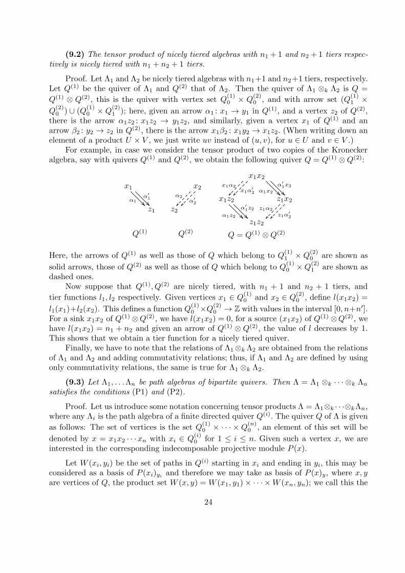
(9.2) The tensor product of nicely tiered algebras with n1 +1 and n2 +1 tiers respec-

tively is nicely tiered with n1 + n2 + 1 tiers.

Proof. Let Λ1 and Λ2 be nicely tiered algebras with n1+1 and n2+1 tiers, respectively.Let Q(1) be the quiver of Λ1 and Q(2) that of Λ2. Then the quiver of Λ1 ⊗k Λ2 is Q =

Q(1) ⊗ Q(2), this is the quiver with vertex set Q(1)0 × Q

(2)0 , and with arrow set (Q

(1)1 ×

Q(2)0 ) ∪ (Q

(1)0 × Q

(2)1 ); here, given an arrow α1 : x1 → y1 in Q(1), and a vertex z2 of Q(2),

there is the arrow α1z2 : x1z2 → y1z2, and similarly, given a vertex x1 of Q(1) and anarrow β2 : y2 → z2 in Q(2), there is the arrow x1β2 : x1y2 → x1z2. (When writing down anelement of a product U × V , we just write uv instead of (u, v), for u ∈ U and v ∈ V .)

For example, in case we consider the tensor product of two copies of the Kroneckeralgebra, say with quivers Q(1) and Q(2), we obtain the following quiver Q = Q(1) ⊗Q(2):

x1

z1

......................................................................... ............

......................................................................... ............α′

1α1

Q(1)

x2

z2

....................................................

....................................................

α2α′

2

Q(2)

x1x2

x1z2 z1x2

z1z2

......................................................................... ............

......................................................................... ............

......................................................................... ............

......................................................................... ............

....................................................

....................................................

....................................................

....................................................

x1α2x1α

′

2 α1x2

α′

1x2

α1z2

α′

1z2 z1α2

z1α′

2

Q = Q(1) ⊗Q(2)

Here, the arrows of Q(1) as well as those of Q which belong to Q(1)1 × Q

(2)0 are shown as

solid arrows, those of Q(2) as well as those of Q which belong to Q(1)0 ×Q

(2)1 are shown as

dashed ones.Now suppose that Q(1), Q(2) are nicely tiered, with n1 + 1 and n2 + 1 tiers, and

tier functions l1, l2 respectively. Given vertices x1 ∈ Q(1)0 and x2 ∈ Q

(2)0 , define l(x1x2) =

l1(x1)+l2(x2). This defines a function Q(1)0 ×Q

(2)0 → Z with values in the interval [0, n+n′].

For a sink x1x2 of Q(1) ⊗Q(2), we have l(x1x2) = 0, for a source (x1x2) of Q(1) ⊗Q(2), we

have l(x1x2) = n1 + n2 and given an arrow of Q(1) ⊗ Q(2), the value of l decreases by 1.This shows that we obtain a tier function for a nicely tiered quiver.

Finally, we have to note that the relations of Λ1⊗k Λ2 are obtained from the relationsof Λ1 and Λ2 and adding commutativity relations; thus, if Λ1 and Λ2 are defined by usingonly commutativity relations, the same is true for Λ1 ⊗k Λ2.

(9.3) Let Λ1, . . .Λn be path algebras of bipartite quivers. Then Λ = Λ1 ⊗k · · · ⊗k Λn

satisfies the conditions (P1) and (P2).

Proof. Let us introduce some notation concerning tensor products Λ = Λ1⊗k · · ·⊗kΛn,where any Λi is the path algebra of a finite directed quiver Q(i). The quiver Q of Λ is given

as follows: The set of vertices is the set Q(1)0 × · · · × Q

(n)0 , an element of this set will be

denoted by x = x1x2 · · ·xn with xi ∈ Q(i)0 for 1 ≤ i ≤ n. Given such a vertex x, we are

interested in the corresponding indecomposable projective module P (x).

Let W (xi, yi) be the set of paths in Q(i) starting in xi and ending in yi, this may beconsidered as a basis of P (xi)yi

and therefore we may take as basis of P (x)y, where x, yare vertices of Q, the product set W (x, y) = W (x1, y1)× · · · ×W (xn, yn); we call this the

24

path basis of P (x). In particular, we see: a vertex y belongs to the support of P (x) if andonly if there are paths starting at xi and ending in yi, for 1 ≤ i ≤ n.

Now assume that Q(i) a bipartite, thus any path in Q(i) is of length at most 1, thuseither a vertex or an arrow. We want to describe the representation 2P (x) for any vertexx = x1 . . . xn of Q. Note that the support quiver of 2P (x) will again be bipartite. We canassume that t of the vertices xi are sources, and the remaining ones sinks. Thus, up toa permutation we can assume that x = x1 · · ·xn with sources xi for 1 ≤ j ≤ t and sinksxj = zj for t + 1 ≤ j ≤ n. The support S of the socle of P (x) consists of the verticesz = z1 · · · zn where zi is a sink in the quiver Q(i) such that there is a path from xi to zi,for any 1 ≤ i ≤ t.

Given an n-tuple u1u2 · · ·un where the ui are elements of some sets (say of ver-tices or arrows of some quivers), and vj is a further element, then we denote by u[vj =u1 . . . uj−ivjuj+1 · · ·un the element obtained from u by replacing its entry at the positionj by vj .

Using this notation, the vertices in the support of 2P (x) with tier number 1 are of theform y = z[xj and the arrows of the support are of the form z[αj , always with z ∈ S, andwith arrows αj : xj → zj , and 1 ≤ j ≤ t.

If we are interested in the structure of P (x), we may assume that all the vertices xj aresources, thus that t = n (namely, if for example xn is a sink, then P (xn) is one-dimensionaland thus P (x) = P (x1 · · ·xn−1)⊗k P (xn) can be identified with the (Λ1 ⊗k · · · ⊗k Λn−1)-module P (x1 · · ·xn−1)).

Given a vertex x of Q, we may look at the coefficient quiver Θ(x) of P (x) withrespect to its path basis (for the definition, see [R2]). If we look at our example of thetensor product of two copies of the Kronecker algebra, and consider the unique sourcex = x1x2 of Q, then the coefficient quiver Θ(x) of P (x) with respect to the path basislooks as shown on the right:

x1x2

z[x1 z[x2

z

......................................................................... ............

......................................................................... ............

.................................................................................... ............

.................................................................................... ............

....................................................

....................................................

.........................................................

.........................................................

x1α2x1α

′

2 α1x2

α′

1x2

z[α1

z[α′

1 z[α2

z[α′

2

Q

x1x2

x1α2 x1α′2 α1x2 α′

1x2

α1α2 α1α′2 α′

1α2 α′1α

′2

............................................................................................................ ............

......................................................................... ............

...................................................................

.................................................................................... ............

.......................................................................................................................................................... ............

........................................................................................................................................................................................................................ ............

....................................................

........................................................................

.....................................................................................................................................

.....................................................................................................................................

........

........

........

.................

........

........

........

.................

Θ(x)

On the left, we present again the quiver of Q = Q(1) ⊗ Q(2), but now using the notationz[? for the vertices with tier number 1 as well as the arrows ending in z.

Now we are going to look at 2P (x) Let z ∈ S and take an arrow αj : xj → zj , lety = z[xj , this is a vertex with tier number 1. The vector spaces P (x)y, P (x)z and thelinear map P (x)z[αj

are given as follows: Since z belongs to S, there is an arrow xi → zifor any i and W (x, z) is a basis of P (x)z (note that here W (xi, zi) is the set of arrowsxi → zi for all i). Similarly, for y = z[xj , the space P (x)y has as a basis the set of elementsof the form α[xj with α ∈ W (x, z), and the linear map z[αj : P (x)y → P (y)z sends α[xj

to α[αj.

25

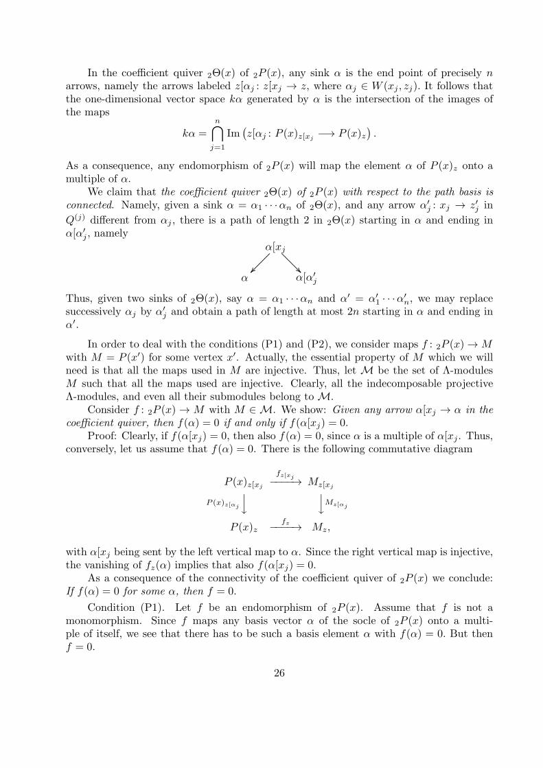
In the coefficient quiver 2Θ(x) of 2P (x), any sink α is the end point of precisely narrows, namely the arrows labeled z[αj : z[xj → z, where αj ∈ W (xj , zj). It follows thatthe one-dimensional vector space kα generated by α is the intersection of the images ofthe maps

kα =n⋂

j=1

Im(

z[αj : P (x)z[xj−→ P (x)z

)

.

As a consequence, any endomorphism of 2P (x) will map the element α of P (x)z onto amultiple of α.

We claim that the coefficient quiver 2Θ(x) of 2P (x) with respect to the path basis is

connected. Namely, given a sink α = α1 · · ·αn of 2Θ(x), and any arrow α′j : xj → z′j in

Q(j) different from αj , there is a path of length 2 in 2Θ(x) starting in α and ending inα[α′

j, namely

α

α[xj

α[α′j

.....................................................................................

......................................................................... ............

Thus, given two sinks of 2Θ(x), say α = α1 · · ·αn and α′ = α′1 · · ·α

′n, we may replace

successively αj by α′j and obtain a path of length at most 2n starting in α and ending in

α′.

In order to deal with the conditions (P1) and (P2), we consider maps f : 2P (x)→Mwith M = P (x′) for some vertex x′. Actually, the essential property of M which we willneed is that all the maps used in M are injective. Thus, let M be the set of Λ-modulesM such that all the maps used are injective. Clearly, all the indecomposable projectiveΛ-modules, and even all their submodules belong toM.

Consider f : 2P (x)→ M with M ∈ M. We show: Given any arrow α[xj → α in the

coefficient quiver, then f(α) = 0 if and only if f(α[xj) = 0.Proof: Clearly, if f(α[xj) = 0, then also f(α) = 0, since α is a multiple of α[xj. Thus,

conversely, let us assume that f(α) = 0. There is the following commutative diagram

P (x)z[xj

fz[xj

−−−−→ Mz[xj

P (x)z[αj

y

y

Mz[αj

P (x)zfz

−−−−→ Mz,

with α[xj being sent by the left vertical map to α. Since the right vertical map is injective,the vanishing of fz(α) implies that also f(α[xj) = 0.

As a consequence of the connectivity of the coefficient quiver of 2P (x) we conclude:If f(α) = 0 for some α, then f = 0.

Condition (P1). Let f be an endomorphism of 2P (x). Assume that f is not amonomorphism. Since f maps any basis vector α of the socle of 2P (x) onto a multi-ple of itself, we see that there has to be such a basis element α with f(α) = 0. But thenf = 0.

26

Condition (P2). Assume there is given a non-zero homomorphism f : 2P (x) → Mwith M ∈ M. Assume that f(P (x)z[xj

) = 0. Of course, then also f(P (x)z) = 0. Thus, itfollows again that f = 0.

Thus we see: if there is a non-zero homomorphism f : 2P (x) → P (x′), then all theelements z[xj with 1 ≤ j ≤ t are in the support of P (x′), and therefore x′

j = xj . It followsthat P (x) is a submodule of P (x′).

Remark: An alternative way for proving Theorem 9.1 is as follows. First, consider thespecial case where none of the quivers Q(i) has multiple arrows. Under this assumptionall the indecomposable projective Λ-modules are thin, thus we do not have to worry aboutbases. The general case can then be obtained from this special case using covering theory.

(9.4) Corollary. Let Λ1, . . .Λn be path algebras of representation-infinite bipartite

quivers. The algebra Λ = Λ1 ⊗k · · · ⊗k Λn has representation dimension precisely n+ 2.

Proof. This follows directly from the inequalities 7.5 and and 9.1.

The special case of the 2-fold tensor power of the Kronecker algebra has been exhibitedby Oppermann in [O2], when he considered one-point extensions of wild algebras. Thisexample was the starting point for our investigation.

References

[APT] Assem, I., Platzek, M.I., Trepode, S.: On the representation dimension of tilted andlaura algebras, J. Algebra 296 (2006), 426-439.

[A] Auslander, M.: The representation dimension of artin algebras. Queen Mary Col-lege Mathematics Notes (1971). Republished in Selected works of Maurice Auslander.

Amer. Math. Soc., Providence 1999.[AB] Auslander, M., Bridger, M.: Stable Module Theory. Memoirs Amer. Math. Soc. 94

(1969).[AR1] M. Auslander, I. Reiten: Stable equivalence of dualizing R-varieties: III. Dualizing

R-varieties stably equivalent to hereditary dualizing R-varieties. Adv. in Math. 17(1975), 122-142.

[AR2] M. Auslander, I. Reiten: Stable equivalence of dualizing R-varieties: V. Artin algebrasstably equivalent to hereditary algebras. Adv. in Math. 17 (1975), 167-195.

[Bs] Bass, H.: Finitistic dimension and homological generalization of semiprimary rings.Trans Amer. Math. Soc. 95 (1960), 466-488.

[Bt] Bautista, R.: On algebras of strongly unbounded representation type. Comment. Math.Helv. 60 (1985), 392-399.

[Bi] BIREP-Workshop 2008: The Representation Dimension of Artin Algebras.http://www.math.uni-bielefeld.de/∼sek/2008/

[Bo] Bongartz, K.: Indecomposables are standard. Comment. Math. Helv. 60 (1985), 400-410.

[Bo2] Bongartz, K.: Indecomposables live in all smaller lengths. Preprint. arXiv:0904.4609[CE] Cartan, H., Eilenberg, S.: Homological Algebra. Princeton University Press, (1956).[CP] F. Coelho, M. I. Platzeck: On the representation dimension of some classes of algebras.

J. Algebra 275 (2004), 615-628.

27

[EHIS] K. Erdmann, Th. Holm, O. Iyama, J. Schroer: Radical embeddings and representationdimension. Adv. in Math. 185 (2004), 159-177.

[G] Gabriel, P.: The universal cover of a representation-finite algebra. In: Representationsof Algebras. Springer LNM 903 (1981), 68-105.

[HU] Happel, D., Unger, L.: Representation dimension and tilting. Journal Pure Appl. Al-gebra 215 (2011), 2315-2321.

[IT] Igusa, K., Todorov, G.: On the finitistic global dimension conjecture for Artin algebras.Fields Institute Communications, vol. 45, 2005, 201-204.

[I] Iyama, O.: Finiteness of representation dimension. Proc. Amer. Math. Soc. 131 (2003),1011-1014.

[J] Jans, J.P.: Rings and Homology. Holt, Rinehart and Winston. New York 1964.[L] Leszczynski, Z.: On the representation type of tensor product algebras, Fund. Math.

144 (1994), 143-161.[LS] Leszczynski, Z., Skowronski, A.: Tame tensor products of algebras, Colloq. Math. 98

(2003), 125-145.[O1] Oppermann, S.: Lower bounds for Auslander’s representation dimension. Duke Math.

J. 148 (2009), 211-249.[O2] Oppermann, S.: Wild algebras have one-point extensions of representation dimension

at least four. J. Pure Appl. Algebra 213 (2009), no. 10, 1945-1960.[O3] Oppermann, S.; Representation dimension of quasi-tilted algebras. J. Lond. Math.

Soc. (2) 81 (2010), 435-456.[O4] Oppermann, S.: Private communication, May 6, 2008.[R1] Ringel, C. M.: Tame algebras and integral quadratic forms. Springer LNM 1099.[R2] Ringel, C.M.: Exceptional modules are tree modules. Lin. Alg. Appl. 275-276 (1998)

471-493[R3] Ringel, C.M.: The torsionless modules of an artin algebra. Selected Topics WS 2007/8.

http://www.math.uni-bielefeld.de/ ringel/opus/torsionless.pdf[R4] Ringel, C.M.: Iyama’s finiteness theorem via strongly quasi-hereditary algebras. Jour-

nal of Pure and Applied Algebra 214 (2010) 1687-1692.[R5] Ringel, C.M.: Indecomposables live in all smaller lengths. Bulletin of the London

Mathematical Society 2011; doi: 10.1112/blms/bdq128[R6] Ringel, C.M.: The minimal representation-infinite algebras which are special biserial.

To appear in: Representations of Algebras and Related Topics, EMS Series of CongressReports, European Math. Soc. Publ. House, Zurich, 2011

[Rq] Rouquier, R.: Representation dimension of exterior algebras, Inventiones Math. 165(2006), 357-367.

[X1] Xi, Ch.: On the representation dimension of finite dimensional algebras. Journal ofAlgebra, 226, (2000), 332-346.

[X2] Xi, Ch.: Representation dimension and quasi-hereditary algebras. Advances in Math.168 (2002), 193-212.

Claus Michael Ringel

Department of Mathematics, Shanghai Jiao Tong University

Shanghai 200240, P. R. China, and

King Abdulaziz University, P O Box 80200, Jeddah, Saudi Arabia.

e-mail: ringel@math.uni-bielefeld.de

28