arX

iv:g

r-qc

/050

8100

v3 2

5 Fe

b 20

06

On the quantum origin of the seeds of cosmic

structure

Alejandro Perez1,2∗, Hanno Sahlmann1,4†, and Daniel Sudarsky1,3‡

1. Institute for Gravitational Physics and Geometry,

Penn State University2. Centre de Physique Theorique, Universite de Marseille

3. Instituto de Ciencias NuclearesUniversidad Nacional Autonoma de Mexico

4. Spinoza Institute, Universiteit Utrecht

March 16, 2018

Abstract

The current understanding of the quantum origin of cosmic struc-ture is discussed critically. We point out that in the existing treat-ments a transition from a symmetric quantum state to an (essentiallyclassical) non-symmetric state is implicitly assumed, but not specifiedor analyzed in any detail. In facing the issue we are led to concludethat new physics is required to explain the apparent predictive powerof the usual schemes. Furthermore we show that the novel way oflooking at the relevant issues opens new windows from where relevantinformation might be extracted regarding cosmological issues and per-haps even clues about aspects of quantum gravity.

∗perez@gravity.psu.edu†h.sahlmann@phys.uu.nl‡sudarsky@nuclecu.unam.mx

1

1 Introduction

The origin and evolution of the large scale structure of the universe consti-tutes a central aspect of cosmology. The widespread view is that our un-derstanding of this aspect has developed dramatically in recent times, boththrough the collection of high precision data in observational cosmology [1],and through better theoretical understanding [2, 3]: The observations arein very good agreement with the theoretical predictions based on the scaleinvariant (Harrison-Zeldovich) spectrum of seed fluctuations and their sub-sequent evolution. Such a scale free spectrum would be hard to explain instandard cosmology because physical processes in the very early universethat might produce it, would have to act on scales larger that the Hubbleradius.This problem is absent if one considers inflationary cosmology, whichseems needed as well in order to deal with well known puzzles arising instandard cosmology [4].

What is more, inflation produces a scale free spectrum of quantum me-chanical fluctuations for the quantized inhomogeneous component of the in-flaton field, and thus seems to give birth to these seeds of structure througha quantum process.

It seems that we have in fact here one of the big successes of theoreti-cal physics in recent times (besides the remarkable, and undisputed achieve-ments that it signifies for observational cosmology), and these facts are widelyviewed as confirmation of an inflationary stage in the very early universe.1

In the present paper, we will be concerned with one specific part of thepicture summarized above, namely the suggestion that inflation not only pro-vides a satisfactory understanding of the evolution of the inhomogeneities,but even an explanation of their origin: The observed similarity between thespectral properties of the (classical) density fluctuations in the early universeand the quantum mechanical fluctuations of the inflaton field after inflationindeed suggest much more than a coincidence. However, we want to drawattention to the fact that a detailed understanding of the process that leadsfrom the quantum mechanical to the classical fluctuations is lacking. Whatis needed to justify the connection between the two spectra is a mechanismthat transforms quantum mechanical uncertainties into classical density fluc-tuations.

1Note however that recent observations indicate an anomalous lack of power at largeangular scales, a fact that has lead to some workers in the field to start questioning theviability of the inflationary model [6]. See also the alternative explanation in [5].

2

This issue has in fact been treated by many authors (see [7, 8, 9, 10, 11,13, 16, 17, 18, 23] for example), most of whom seem to suggest that the sub-ject has been clarified and thus, at least on a fundamental level, possessesno further mystery. Indeed most of the proposals seem to invoke nothingbeyond standard physics to explain the coincidence of the spectra. On theother hand this same body of literature can be considered as an indicationthat underneath all of the reassurances to the contrary, there is a remain-ing degree of discomfort, and certainly the fact that the different authorspoint to slightly different schemes for this quantum to classical transmuta-tion, indicates that each author does not find the schemes espoused by theircolleagues to be fully satisfactory. Indeed we feel that, at least on a funda-mental or conceptual level, the treatments proposed are missing something,and we will try to pinpoint the place where there is a missing step in themost well known ones. This will lead us to argue that in fact somethingbeyond standard physics seems to be required if the essential picture and itssuccessful degree of predictive power is to be preserved. At the same time weunderscore the richness of the physical information that is being overlookedwhen the problem is not addressed head on.

To illustrate the physics behind that missing aspect, we introduce a sim-ple phenomenological model involving a dynamical collapse of the wave func-tion as the mechanism that leads to the transition to inhomogeneity. It isphenomenological in the sense that it does not explain the transition to in-homogeneity by some particular new physical mechanism, but merely givesa rather general parametrization of such a transition. We will briefly discusssome of the characteristics that the new physics would have to include ifwe wanted it to justify our analysis. We also show how the value of someparameters can be studied by comparisons with observational data.

Since one is ultimately dealing with connecting quantum mechanical quan-tities to measurement results, one might be tempted to consider the issuedescribed above as related to old and well known interpretational problemsof Quantum Mechanics, and thus to dismiss it as inconsequential as far asthe physical predictions for observations are concerned. After all, these in-terpretational problems of Quantum Mechanics can be mentioned in everyinstance where use of the theory is made, and we have all grown accustomedto the fact that, in practice, those issues have no incidence whatsoever onour ability to make correct predictions. We will argue that quite to the con-trary, the situation at hand, namely the cosmological setting, is such thatthe way one deals with these issues could have an impact on the predictions

3

for observations. Furthermore, the standard rules that one can rely on, tosettle all practical ambiguities in ordinary quantum mechanical situations,are not available in the present case. The reasons for these differences arethreefold: First the object that is being treated quantum mechanically is theentire universe, and thus the standard separation of the system into subsys-tem of interest, observer, and environment, becomes unjustifiable and wouldbe in fact subject to completely capricious choices. Second, that we haveat our disposal just a single system – our universe –, so the recourse to thestatistical ensemble interpretation of the result of a measurement in quantummechanics is not directly available. And third the fact that not only do theobservations pertain to the very late causal future of the assumed quantumto classical transition, but in fact the existence of the observers themselvesdepends upon the outcome of the measurements. In our view these factsindicate, not only, that this aspect of cosmology offers a rather unique op-portunity to focus on these so called “interpretational aspects of quantumtheory” – and to look for clues that might lead to a better understanding ofthem – but point in fact to the conclusion that any satisfactory treatment ofit requires a step beyond what we currently have as established interpreta-tional models of quantum mechanics. We will refer to this unknown aspectas new physics.

The article is organized as follows: In Section 2 we review the standarddescription of the inflationary scenario for the origin of the seeds of cosmicstructure. In Section 3 we make a general critique of the standard description.In Section 4 we critically discuss the main ideas that have been put forwardregarding the transition to classicality. In Section 5 we point out the natureof the missing element and propose some ideas. In Section 6 we review thedescription of linearized fluctuations maintaining the framework that seemsnecessary to make our proposals in a clear and transparent manner. InSection 7 we proceed to make the quantum mechanical treatment of thefield fluctuations within the setting necessary for implementing our ideas.In Section 8 we show how to implement our proposal within the standarddiscussion of the origin of the seeds of cosmic structure. In Section 9 werecover the predictions that must be compared with observational results.Section 10 contains comments and calculations into some further directions,and we end in Section 11 with a discussion of our conclusions.

Regarding notation we will use signature (-+++) for the metric andWald’s convention for the Riemann tensor. We will use units where c = 1but will keep the gravitational constant and h explicit throughout the paper.

4

2 The standard picture

As mentioned in the introduction there are many treatments of the subjectdiffering in technical as well as conceptual aspects. However, they do sharea “standard core” which we resume here for the benefit of the reader, withno ambition toward completeness or rigor2.

1) Start with the action of a scalar field coupled to gravity.3

S =∫d4x

√−g[ 1

16πGR[g]− 1/2∇aφ∇bφg

ab − V (φ)], (1)

where g is the space-time metric and φ the inflaton scalar field.2) One splits the fields (g, φ) into a homogeneous-isotropic background

plus an arbitrary fluctuation assumed to be small, i.e. g = g0+δg, φ = φ0+δφ.The background geometry g0 is assumed to be the Robertson Walker space-time

ds2 = −dt2 + a(t)2(dx21 + dx22 + dx23), (2)

where a(t) is the scale factor and t is the cosmological time. Note that forsimplicity we have restricted attention to the case of flat spatial slices (k = 0in the usual notation). The homogeneous and isotropic background field φ0

satisfies the equation of motion gab0 ∇a∇bφ0 + ∂φV [φ0] = 0 which due to thesymmetry assumptions becomes

φ′′0 + 3

a′

aφ′0 + ∂φV [φ0] = 0, (3)

where primes indicate derivatives with respect to ordinary cosmic time t. Thesecond term acts as a friction term. One assumes the so-called slow rollingcondition φ′′

0 = 0 (for an analogy think of the motion an object falling withterminal velocity under the influence of gravity in a viscous medium). Theenergy-momentum tensor of the background field is thought to be dominatedby the potential term, so one takes it to be approximated by

T(0)ab [φ0] = V [φ0]gab.

2The reader can use for instance [12] as an up to date review of the subject3That we can assume the universe to be devoid of matter except for the scalar field is

in fact the result of the early inflationary period that is thought to precede the regime weare describing.

5

To achieve slow rolling, the potential has to be sufficiently flat in the regionwhere the initial conditions for φ0 are set. Consequently Einstein’s equationsimply that during the inflationary regime we have:

a(t) = AeHt, φ(t) = φ0(t) = φinitial + φ′0t (4)

where H =√(4/3)πGV0 and V0 = V [φinitial], using the fact that during the

regime of interest the potential is essentially constant.3) Now, turn to the fluctuations, and concentrate on the matter sector:4

The scalar field δφ(x) can be treated as a standard, scalar field on the back-ground (2). It is useful to decompose it into Fourier modes, since they areuncoupled due to the symmetry of the background. For simplicity we intro-duce an infra-red cutoff by assuming the spatial slices to be Σ := [0, L]3, i.e.a box of length L. Then the total Lagrangian for δφ (derived from (1)) canbe written as a sum of mode Lagrangians

Lk =a3

2

[|δφ′

k|2 −k2

a2|δφk|2

](5)

for the modes δφk =∫L3 exp(−ikx)δφ(x) (with kiL/(2π) ∈ Z (i = 1, 2, 3)).

During inflation the equations of motion from (5) become

δφ′′k + 3 H δφ′

k −(k

a

)2

δφk = 0, (6)

where one is using that Einstein’s equations imply a′/a = H in that regime.We remind the reader that at this point one is not indicating that there areinhomogeneities of any definite size in the inflationary universe, but merelyone is considering what would be the dynamics of any such small inhomo-geneity if it existed. The issue of their presence and magnitude is dealt withat the quantum level, where the fluctuation field is just an operator, and theabove mentioned matter is associated with the state of such quantum field.In fact, the next step is the quantization of the field. Note that in terms ofthe Fourier modes, the Hilbert space for the quantum field will be a directproduct of Hilbert spaces – one for each mode.

4A more detailed treatment would also involve discussion of the metric perturbations,and issues of gauge. Note also that in some more recent treatments [13], quantization isapplied directly to a gauge invariant combination of scalar field and metric perturbations.

6

4) For quantization, one needs to chose a vacuum state for the field andassume it represents the initial state at the onset of inflation. This stateis required to be homogeneous (i.e. all n-point functions are invariant undertranslations and rotations in the spatial slice). After all, the point is toexplain the emergence of the inhomogeneities, rather than merely to assumetheir presence at the onset of inflation and to study their evolution. There isan obvious problem in this step, because the choice of a vacuum state is notunique in space-times that do not possess a time-like Killing field. Though adifficult issue in principle, in practice the results do not depend much on thechoice of the initial state as long as it approaches a canonical form for modesδφk with large k. In the literature a sort of “instantaneous vacuum state” ismost often chosen as the initial state. In the way we presented things here,this corresponds to the assumption that at the onset of inflation the wavefunctions for the mode δφk and its canonical momentum πk are Gaussianwith spreads

(∆δφk)2 =

1

2a2k, (∆πk)

2 =ha2k

2. (7)

For k >> aH the friction term in (6) can be neglected and thus the timeevolution of the mode δφk is just that of a harmonic oscillator (with timedependent mass). Then the above choice just amounts to the modes startingout in the ground state of a standard harmonic oscillator.

5) Time evolution of the quantum state: As described above, a modeinitially corresponding to k >> aH is assumed to start out in the groundstate. As a grows larger the proper wave length of the mode will reach theHubble radius (k = aH) and the friction term in (6) will start dominatingthe dynamics. As the wave length grows larger one can approximate thesolution to (6) by an over-damped oscillator and the value of the field can beassumed to be frozen at its value at Hubble radius crossing. At that momenta = k/H so that the fluctuations of δφ and πk can be approximated by

(∆δφk)2 =

H2

2k3, (∆πk)

2 =hk3

2H2. (8)

6) Now the fluctuations (8) are identified with (or, in a more careful for-mulation such as in [14], “taken as indicative of”) the (classical) spectrum ofinhomogeneities. For example, often the fluctuations of the energy densityin co-moving coordinates, δρ, is used as a measure for the classical inhomo-geneities. It is easily verified that δρ ∼ φ′

0a−3πk. Thus one sets

|δρk|2 ∼ a−6(∆πk)2 ∼ k−3 (9)

7

at the time the mode k leaves the Hubble horizon. δρ is understood as aclassical quantity.

7) The classical density fluctuations are now evolved through the end ofinflation and into the regime of standard cosmology. It can be shown thatthe spectrum of the fluctuations at the time they exit the Hubble radiusis proportional to the spectrum at the time they re-enter. Thus one has(δρk)enter ∼ k−3/2 which is the scale free Harrison-Zeldovich spectrum. Theclassical fluctuations are then evolved further to take into account the matterdynamics, leading to the famous acoustic peaks.

8) The resulting evolved spectrum is compared with the observations ofthe CMB. Furthermore, these departures from homogeneity and isotropy arethought to be the seeds for the evolution of the structure that we see in theour universe, and that are in fact necessary for our own existence.

This is in essence the standard account of the process for obtaining theseeds of cosmic structure formation that forms the basis of the analysis ofcosmological data, and in particular of the CMB anisotropies.

3 A critique of the story

The previous analysis is remarkable: The universe starts in a homogeneousstate and ends up with inhomogeneities that fit the experimental data. How-ever, as we will argue in the following sections, this is not fully justifiable by“standard physics”. We should point out from the start that many authorsdo acknowledge the existence of a gap in our understanding, for instance[14, 15], and some do propose ways to deal with the issue in more detail (seeex. [7, 8, 11, 29, 36]). There is also a large literature on issues of quantummechanics in the context of cosmology in general (ex. [10, 16, 24, 27]). Thediscussion that follows is addressed to those colleagues that are not fullyaware of the problem, and to those that believe that there is no problem atall.

The first point that we want to make is that the above analysis can notbe justified through standard quantum mechanical time evolution. If this isnot already obvious from the particulars of step 6, just note that as alreadystated above, the initial quantum state is symmetric5 (i.e., homogeneous and

5The vacuum state defined in step 4 is invariant under the action of the symmetry groupof the background. Even though it can be written as a superposition of states which are

8

isotropic) and the standard time evolution does not break this symmetry,thus it can not explain the observed inhomogeneities. The states obtainedin other natural schemes, such as the one arising from the “No Boundary”boundary condition in quantum cosmology are equally homogeneous andisotropic, as can be seen explicitly in eq 8.6 and 8.9 in [17].

Let us now look at step 6 in more detail: The essence seems to be that aclassical quantity is identified with (the square root of) a quantum mechanicalexpectation value. This suggests that one might be able to view the procedureof step 6 in the framework of a semiclassical theory, i.e. one in which apart of the system is described classically, while another part is describedquantum mechanically. A hallmark feature of such type of descriptions isthat classical quantities are coupled to the quantum sector via expectationvalues. While not satisfactory as fundamental theories, they neverthelessoften have some validity as effective theories. However, we note that twothings are remarkable about the prescription of step 6 and set it apart fromsemiclassical theories such as semiclassical gravity: a) In step 6 a classicalquantity couples to the square-root of the expectation value of the square ofits quantum counterpart. b) The use of Fourier transforms in step 6. Thechoice involved in a) is certainly not the simplest possibility, and not the onechosen in standard semiclassical treatments. Point b) would not be an issue ifthe relation were linear, but raises concern due to the choice made in a). Forinstance, what if instead of plane waves one uses spherical harmonics in themode expansion? The non linear nature of a) implies that this will affect theresult. Note also that both a) and b) must be required to achieve the result ofthe standard view described in the previous section. If we drop any of the twowe do not get the sought-for inhomogeneities. For instance, identifying thesquare root of the expectation value of δφ2(x) with the classical counterpart(i.e. dispensing with b)) leads to a result that is independent of x, and thusit is homogeneous. Identifying the expectation value of φk with its classicalcounterpart (i.e. dispensing with a)), leads to a homogeneous result (zero,in fact) as well.

One quite often reads the following argument to support a) and b): Asimple calculation shows that < φ2

k > is equal to the Fourier transform ofthe auto-correlation of the two-point function of φ(x), and thus quantifies

not symmetric by themselves the superposition does not select any direction and looks thesame at every point on the homogeneous t =constant slices. This is completely analogousto the Poincare invariance of the standard vacuum on Minkowski space-time.

9

correlations of the field at different points. The observations are then arguedto be a measurement of these correlations, because one is measuring thedifferences in the temperature of the CMB between different directions inthe sky. We do not find this convincing however, because although WMAPin fact works as a differential thermometer, it does so in a way that allows oneto obtain a map of the temperatures in the sky, and it is this map which issubjected to a Fourier analysis from which the observational power spectrumis read.6

One may want to interpret step 6 as an effective description of some sortof measurement process or “collapse of the wave function”. This seems tobe plausible, as step 6 involves expectation values of squares of operators,i.e., quantities that measure the spread of measurement results according tostandard quantum mechanics. Furthermore, a measurement can break thesymmetry of the initial state and produce, in our case, inhomogeneities. Thisscenario would be quantum mechanics at its core: The unitary evolution (theU process in [19]) of the quantum state with a symmetry preserving Hamilto-nian will not break the initial symmetry of the state, but a measurement of anobservable whose eigenstates are not symmetric, forces the system (throughthe collapse, called R process in [19]) into one of the possible asymmetricstates. The onset of the asymmetry (in standard interpretations of quan-tum mechanics) occurs only as a result of the measurement, and then, onlywhen the measured observable does not commute with the generators of thesymmetry.

However this scheme, applied to the situation at hand, immediately raisesmany questions: What constitutes the measurement in our cosmological sit-uation? When did it happen? What is the observable that was measured?Perhaps the answer is somehow connected to our own observation of the sky?Are we to believe that until 1992 [20] the CMB was in fact perfectly homo-geneous? Hardly, as we know the conditions for our own existence dependon the departures from homogeneity and isotropy in our universe, and thusour actions could not be their cause.

Moreover, the predictive power of quantum mechanics regarding one sin-gle measurement is rather small (in the EPR case the only absolute prediction

6After all, if it were technically possible to replace the comparison of temperatures attwo different points in the sky with, say, the comparison of the temperature of a singlepoint in the sky with the temperature of a reference body within the satellite, one wouldnot expect the resulting temperature map to change (unless one is prepared to argue theCMB really is a quantum system in a higly non-classical state).

10

for one experiment concerns to the situation in which the two measuring axesare perfectly aligned). How is it, then, that we have such a predictive powerin regards to the single measurement of our sky? One could think that this isdue to the fact that we are measuring many regions in the sky and that eachshould be considered as a different measurement, but this is not the case:The measurement of the amplitude in one single mode requires the Fouriertransform on the whole sky. The fact that the actual measurements involve(for technical reasons) smaller regions than that, is in fact responsible foruncertainties in the measurement of the quantity of interest.

Step 6 might effectively describe some sort of measurement, but importantquestions have to be answered:

1. What is performing the measurement?

2. Precisely, what is the set of quantum observables that is being mea-sured? And what determines them?

3. When is this measurement taking place?

4. Can the above questions be answered in such a way that the ensuingpredictions are in agreement with observations.

One further issue that needs discussion is the nature of the different av-erages, fluctuations and in general statistical issues that are present in theproblem and that are sometimes treated as if no differences even of princi-ple did exist. First we have the quantum mechanical aspect of the problem,reflected for instance, in the evaluation of expectation values of observables.Here the statistical nature is reflected in the usual indeterminacy of futuremeasurements of certain quantities when the state of the system does notcoincide with an eigenstate of the observable. However let us imagine for asecond that we could find an operator that measured the degree of cosmicinhomogeneity of the system. It is clear that the vacuum would correspondto an eigenstate of such operator with zero eigenvalue. If that was the observ-able that is measured, the inescapable result would certainly be problematicfor the standard analysis that is supposed to lead to the observed spectrumof fluctuations. The point is not to discuss whether this operator exists ornot but to note that the statistical aspect associated with the quantum me-chanical picture would emerge only when the particular observable associatedwith a measurement is selected. Next we have the statistics associated with

11

the classical ensemble represented by the stochastic field and the correspond-ing inhomogeneities characterizing the corresponding ensemble of universes.And finally we have the statistical description of the inhomogeneities withinour own universe, which can be thought of as an arbitrary generic realizationwithin the ensemble of universes mentioned before. Here the point is to dis-tinguish in principle, between the statistics in the ensemble of universes, andthe statistics within one (our own). We are used from our experience withstatistical mechanics to identify averages over ensembles with physical expec-tations, however we must recall that these identifications rely on two otheridentifications: The identification of the ensemble averages with the longtime averages (a fact that relies on the validity of the ergodic assumptions),and the identification of long time averages, with the results of physical mea-surements, a fact that relies on equilibrium considerations. Needless to say,that none of these conditions are present in the problem at hand. Some ofthese issues have motivated the considerations in [18].

The claim that there exist a prediction regarding the primordial den-sity anisotropies and inhomogeneities in the universe could not be sustainedwithout addressing these questions.

4 A look at proposed ideas on the transition

to classicality

In this section we give a quick overview of the most popular ideas proposedto address these issues, and attempt to exhibit as clearly as possible theirincompleteness, by signaling the point at which a “missing element” makes adisguised appearance, or at least indicating the place where it should have en-tered in order to justify the subsequent interpretation given to the computedquantities.

Standard Decoherence

Decoherence in its standard interpretation describes the fact that when con-sidering a quantum system with a very large number of degrees of freedom,most of which are ignored (by considering them as “the environment”), thedensity matrix for the subset of the remaining, interesting “observables”,evolves under certain circumstances, and after suitable time averaging, to-wards a diagonal matrix. This is sometimes said to represent the emergence

12

of the classical behavior of the interesting observables. There has been cer-tainly a large amount of work on this field, most of it devoted to evaluatingthe time evolution of the previously mentioned density matrix in varioustypes of situations, or more specifically to studying the decoherence func-tional. There is however much less work devoted to interpretational issuesand it is fair to say that decoherence has not solved the measurement problemin quantum mechanics [21]. In fact, the diagonal character of the resultingdensity matrix point to the disappearing of certain quantum aspect of theproblem. That by itself is certainly not enough to claim that the situationhas become completely classical: A non-interfering set of simultaneous co-existing alternatives is not something that can be thought of as belongingto the realm of classical physics. This sort of criticism regarding such inter-pretations of decoherence have of course been made before, for instance seesection, 2.3.4 of [22]. Moreover the diagonal nature of the density matrixwould disappear if we write it using a different basis for the Hilbert space ofthe quantum system, clearly indicating that even this aspect of the so calledclassicality has a limited validity.

Thus, the main issues that confront the decoherence approach to themeasurement problem in quantum mechanics are the selection of the basis,and the fact that after one has a diagonal density matrix, one is in general,still a big step removed from an interaction specific eigenstate for the desiredobservable. In the standard case one can progress beyond this point byinvoking the measurement apparatus to help select the basis, and by using theensemble interpretation to deal with the density matrix. These two aspectsare clearly absent in the cosmological situation we are considering7. In factthe need for going beyond standard quantum mechanics in this context hasbeen noted before [23, 24] (and we will discuss this line of thought furtherat the end of this subsection). Furthermore, if one wants to claim thatdecoherence solves the problem in the cosmological setting at hand, one mustfind a preferential basis selected by a physical mechanism, and a criterion forthe separation of the degrees of freedom into the “interesting set” and “theenvironment” dictated by the physical problem at hand. In some schemesone might be able to unify these two issues into one by arguing that theenvironment determines the relevant basis to be that in which the system

7As we already mentioned, taking the position that the measurement is in fact ourown series of studies of the CMB, leads to a closed circle of causes and effects, with anexplanatory power that is highly doubtful to say the least.

13

apparatus environment interaction is diagonal [27]. In any case, the resultwould then naturally have the imprint of these two inputs – perhaps unifiedinto one – but so far no universally accepted prescription for such choicesexits, nor can such selection be fully justified, in the standard descriptions ofthe origin of the cosmic density fluctuations. For instance, one might want toargue that one needs to trace over the very large wavelength modes, becausethey are unobservable, as is done for instance in [27], but as the part of theuniverse that is observable by a co-moving observer is certainly dependenton the cosmological epoch, the tracing would depend on the cosmic timeof the observer, but as such it can not be argued, unless we do away withcausality, to play a role in the onset of inhomogeneity and anisotropy in theearly universe. Quite generally, we can not allow our own characteristicsand limitations to come in into the argument, if our hope to explain theasymmetries that give rise to the conditions that make our existence possible.

Actually, in some of the treatments invoking decoherence one finds atsome point of the discussion, an appeal to a “a specific realization” ([7] sec.3, [9] sec. V) of the stochastic variables, in a clear allusion to something thatcan be called the “collapse” from the statistical description of the universe,into one of the elements of the statistical ensemble.8 This is the point, ofcourse, when we transit from a homogeneous and isotropic description toan inhomogeneous and anisotropic one, presumably corresponding to ouruniverse. However nothing is said about when and how the transition occursin our universe.

In fact what seems to be an insurmountable issue in this scheme is the fol-lowing: Even if we go from a perfectly symmetric state (the symmetry beinghomogeneity and isotropy), to a density matrix for a subset of the physicaldegrees of freedom, which is expressed in a basis in which the non-diagonalelements are negligibly small, through a justified selection of the degrees offreedom that should be considered environment, one could not end up withan asymmetric mixed state, as there is nothing in the physical laws or the ini-tial situation that could lead to such breakdown of the symmetry. Thus themixed state described by the density matrix is still perfectly symmetric.Thedensity matrix is then given a statistical interpretation, by which we stopregarding the matrix as representing the state of our universe, and insteadview it as representing a statistical ensemble of universes, among which we

8Note that other schemes are based to some degree on this sort of specific realizations,without calling them by this name – see for instance [28]

14

find our own. The ensemble as a whole is clearly symmetric, but leaves roomfor each of the elements in the ensemble to be asymmetric. This is how weend up with an inhomogeneous and anisotropic universe. However, it is clearthat this does not address at all any of the characteristics of transition ofour universe from an initial symmetric state, to such a resulting asymmetricstate. This problem affects all the schemes based on decoherence, includingthe detailed treatments in [29], and if we seek a realistic understanding of theorigin of inhomogeneity and anisotropy in our universe, this approach wouldclearly be missing something.

After this discussion of the difficulty of applying the standard picture ofdecoherence in the cosmological context, we would like to mention the ideasof Hartle and collaborators. We have placed them here even though they callfor a generalization of Quantum Mechanics. In fact, we view his argumentsfor the need of a generalization of Quantum Mechanics to be applicable notonly to quantum gravity, but also to cosmology ([24, 25], and referenceswithin) as further indications for the need to go beyond standard physics.The particular generalization of Quantum Mechanics that has been suggestedinvolves the assignment of a decoherence functional to allowed sets of coarsegrained histories. One such set of coarse grained histories decoheres whenthere is no quantum mechanical interference among the different alternatives.In that situation we are able to assign definite probabilities to the particularalternatives. In the case at hand this would have to be applied to the historiesstarting during the inflation period in early universe to the formation of largestructures and eventually to ourselves.

We should however mention some problematic aspects of this proposal:To start with, the division of the global set of all fine grained histories intosets of coarse grained histories might be done in various ways, leading todifferent decoherent sets [26]. Second, the coarse graining, and correspondingdecoherence, arises only when we ignore certain degrees of freedom, and thejustification for doing so, relies on what we, as humans living in this particularera, could in principle observe and what we can not. This is fine, except inthe case that what we seek to understand is the emergence of the conditionsthat lead to the possibility of our own coming into existence. It is clear thatin that case we can not call upon some of our own characteristics as a partof the explanation.

15

Decoherence without Decoherence

This can be viewed as a particular realization of the ideas of the previouscase. Its main appeal is that one needs to consider only the scalar field andno other physical system is required to play the role of “environment”. Thepoint is that certain modes of the scalar field vanish asymptotically in timeas a result of the inflationary dynamics of the universe. These modes arethen deemed unobservable, and one is then invited to treat them as such,taking the appropriate trace and obtaining a mixed state from what wasinitially a pure quantum state of the field (ex. [7, 8]). This approach notonly suffers from the same drawbacks that affect the decoherence approachin general, but also from what seems as a further interpretational excess:To have expectation values or higher moments of a mode converge to thezero value is not the same as making it unobservable. Zero is just as gooda value for a scalar field as any other one. Moreover it is clear that evenif one would agree on the non observability of certain degrees of freedom,that does not imply necessarily that the system as a whole needs now to betreated as a mixed state. There could be other reasons that fix the state ofthose degrees of freedom. A proton can, in the appropriate circumstances,be described as a pure quantum state, despite the fact that in these sameconditions its microscopic constituents – quarks and gluons – might be, inpractice, unobservable.

One novel aspect that is sometimes invoked in these treatments is thesqueezing of the vacuum [7, 8]. That is, one notes that during the inflation-ary stage the initial vacuum state for each mode, evolves towards a squeezedstate. We recall that a squeezed state is a state that has the minimal uncer-tainty but not in the standard position and momentum variables but a newpair of “rotated” canonical variables. Thus, in our case, one has an uncer-tainty on the value of field and conjugate momentum which is much largerthan the minimum uncertainty provided by quantum mechanics. Thus oneconcludes this minimal uncertainty (indicated by Q.M.) is negligible com-pared with the actual uncertainty and thus that one can neglect quantummechanics. This is taken as an indication that there has been a transitionfrom the quantum to the classical behavior. This conclusion does not seemto be sufficiently justified, as can be seen by noting that in many concrete sit-uations, such as those studied in Quantum Optics, one deals precisely withstates that have uncertainties in conjugate quantities that are larger thanthe minimal ones provided by Q.M. and nevertheless there are situations

16

– for instance when one is interested in experiments sensitive to quantitiesother than the ones in which the system is seen as squeezed – that one musttake into account that one is dealing with a system that must be treatedquantum-mechanically. 9

We conclude that it is clearly insufficient to have the product of theuncertainties being much larger than h as criterion for classicality. Onecould consider instead as criterion for classicality the requirement that thevolume of phase space occupied by the system, as measured for instance bythe support of the Wigner functional, be much larger than h. This conditionis however not satisfied by a squeezed state. For a critical discussion of theseissues in the context of inflation see also [11]10.

And of course we have the other issues that have been pointed out re-garding the general scheme of decoherence as describing the transition froma quantum, homogeneous, and isotropic state of affairs to a classical (orquasi-classical), inhomogeneous and anisotropic situation.

Alternative to Inflation

In a recent work Wald and Hollands [5] have shown that is possible to recoveridentical predictions as those afforded by inflation, regarding the spectrumof the seeds for cosmic structure formation, without requiring the universeto have gone through an inflationary stage. They start by considering againthe dynamics of a scalar field in a background cosmological setting. In theirmodel, the inhomogeneities in the universe originate while the universe isdominated by radiation or dust so that the scale factor grows as a(t) = ctα

with cosmic time t, where c is a constant and α < 1. Their model justrequires that all modes would have been in their ground state (as in the

9The problem can be seen more clearly if we look at the following example. Take anelectron in a minimal wave packet localized at the origin such that the uncertainty in theposition ∆X = α and that in its momentum is ∆P = h/2α. Now construct a superpositionof such state with an identical state after a translation by a large distance D. The productof the uncertainties is now roughly Dh/2α which can be made as big as desired by takingD sufficiently large. Clearly the system is nevertheless far from being classical.

10It is illustrative to mention, in the context of this example, that one might add tothe electrons their spin degree of freedom and consider the state where the electron at theorigin has its spin up, superposed with the displaced state where the spin is down. Nowconsider the density matrix obtained by ignoring the spin degree of freedom, (and thustracing over it). In that case we would have an essentially diagonal density matrix in theposition basis, but one could not argue that one has a classical situation.

17

standard picture), and that the fluctuations are “born” in the ground stateat an appropriate time which is early enough so that their physical length isvery small compared to the Hubble radius, and then they “freeze out” whenthese two lengths become equal. The presentation of their model actuallyallows one to see clearly the need for some process that would be responsiblefor the so called “birth” of the fluctuations, which can be seen to play a rolesimilar to that of quantum mechanical measurement. In fact the so called“birth of the mode” is the step whereby a quantum mechanical uncertainty isreplaced, in their treatment, by an actual classical fluctuation of the energydensity, and the point at which a particular mode that has been contribut-ing in an absolutely homogeneous and isotropic way to the universe density,becomes a source of the inhomogeneities that presumably are responsible forthe structure in the matter distribution of the early universe. The issuesare then: What physical process is responsible for these “births”, or trans-mutation of the fluctuations? And how is it that such process selects theparticularly appropriate time of such occurrence for each particular mode?

The ‘many universes’ perspective

One view that is apparently very widespread among the community workingin inflation (but much less represented in the corresponding literature), iswhat can be called the Many Universes perspective. According to this pointof view, our universe is one among a large number of universes that constitutean ensemble, and it is this ensemble what is in fact characterized by thequantum state that is homogeneous and isotropic. The standard treatmentis then interpreted as reflecting the most likely aspect our universe can beexpected to have, when considered statistically within such an ensemble.In such an interpretation there appear to be no open issues, no need for acollapse, and certainly not new physics.

Note that this would have to be quite different from the Everett, or ManyWorlds, interpretation of Quantum Mechanics. In the latter, reality is madeof a connected weave of ever splitting worlds, each one realizing one of thealternatives that is opened by what we would call a quantum mechanicalmeasurement. It is thus clear that the points of splitting, the basis in whichthe splitting occurs, and the physical entity associated with the triggeringof the splitting are in one to one correspondence with the aspects we havementioned before which are associated with the collapse of the Copenhageninterpretation (time of measurement, basis, and measuring device). In the

18

Many Universes paradigm there is no splitting, as that would have amountedeffectively to a collapse and would then be subjected to the equivalent set ofquestions: When did the splitting occur? What caused it? And how was thebasis in which it happened, selected? In particular, it should be emphasizedthat from such ”Many Universes” point of view, our universe was neverhomogeneous and isotropic. Let us however examine in more detail whatsuch view entails.

In the most direct interpretation of such posture we would have a collec-tion of universes, each one of which has a definite and concrete realization setof the asymmetries (the symmetry being of course homogeneity + isotropy).However, when this is being said, we clearly imply that each one of these uni-verses would be susceptible to have a description, in particular, a descriptionof its asymmetries. That description must be either classical or quantummechanical.

If we take the first option, we would be taking the position that quantummechanics is a theory applicable to ensembles of systems. In this view, wemust confront two aspects, a) each one of the elements of the ensemble canindeed be described in a classical language, and b) the quantum mechanicaldescription contains information only about the statistics that results fromrepeated experimentation applied to the collection of elements constitutingthe ensemble. Aspect b) of this posture, i.e. the applicability of QM only toensembles, is in itself problematic given the absolute nature of the predictionregarding a single system that can be made in certain special circumstances(like when dealing with eigenstates of the operators to be measured or whenthere are superselection rules totally forbidding certain processes), for moreon this issues see [30]. But even more disquieting is aspect a) of the posture,namely the one where one advocates that each member of the ensemble hasa classical description. This position would revert one to a sort of “hiddenvariable” advocacy, which would say for instance that in an EPR set-upeach electron has a well defined value of its spin components even beforethe measurement is done, a position which is known to be untenable in lightof the Bell Inequalities for correlations (See discussion by in [31] and theirexperimental corroboration [32]).

If we take the second option, we would be saying that our universe is ina quantum state, which is not symmetric, but that, when superposed withthe other asymmetric quantum states that describe a certain ensemble ofuniverses, leads to an homogeneous and isotropic quantum state; the onecorresponding to the inflationary field vacuum for the initial stages of infla-

19

tion. This seems fine at first sight, however, it is far from what QuantumMechanics prescribes: One does not superpose a state describing one system,with the state describing a second system to obtain the collective descriptionof the two systems. A further problem appears when we want to take theargument in the opposite direction. Namely, taking as the initial assumptionthat the state that collectively describes the collection of universes is the onecorresponding to the vacuum state of the field and is thus homogeneous andisotropic, one must end up with a decomposition of that state in a particularbasis (of non-symmetric states) of the Hilbert space in order to associate toeach universe a corresponding quantum state. Now we face two issues. First,the election of such basis, is not given “a priori” by the formalism. One cancertainly think of ways to make the choice, and such choice would correspondto the selection of the quantity that is “measured” in ordinary Quantum Me-chanics. This aspect is missing in the standard descriptions. In fact it wouldcorrespond to whatever selects the basis in which the collapse takes placein our approach. The supra-temporal selection of the basis (supra-temporalin the sense that, from this point of view, each universe is from the onsetin a specific non-symmetric quantum state) has no counterpart in ordinaryQuantum Mechanics. For instance when considering an EPR correlated pairof electrons one could not take the position that there is a multiplicity ofuniverses and that in ours each electron is in a specific state of its spin at alltimes along its path. Similarly, when considering an electron in its groundstate in a hydrogen atom one would not argue that in our world the electronis in an eigenstate of the position and that the ground state correspondsin fact to a description of a corresponding ensemble of universes with fullylocalized electrons. This aspect is therefore novel to the situation at hand,and as such would qualify also as New Physics.

The second problematic aspect is the following: In taking this point ofview, our universe would be considered as always having been in a state thatis anisotropic and inhomogeneous. It would have never corresponded to thevacuum state of the scalar field. Then, one might find uncomfortable theidea that placing our universe within an ensemble together with a large setof unobserved universes, one might be able to make predictions about ourparticular one. In other words, if we do not assert that our universe startedin the scalar field’s vacuum, how could we end up with prediction for itsanisotropy that takes such a state as the starting point? Some readers mightargue that this is an epistemological complaint, and dismiss it, while otherswould sympathize with the uneasiness. In any event it is worth noting that

20

this aspect is there.The final option that seems to be open within this general point of view

asserts that our universe was indeed, together with all the elements in the en-semble in the start corresponding to the homogeneous and isotropic vacuumstate of the scalar field. That all these possibilities thus evolved “simultane-ously” and that in each one of them (or at least in a great many of them)structures such as galaxies and stars formed out of the initial asymmetries,and that observers like ourselves then evolved in some of the solar systems,and that these observers thus carried out the observations that selected thebasis in which a standard type of measurement-induced collapse occurred.The problem of course is that only in very special basis would the galaxiesstars and observers themselves exist to carry out the observations that effectthe measurement-like collapse and concomitant selection of the basis.

Finally, and as a cautionary note against the hope of finding a coherentand orthodox description of the situation, one should keep in mind the factthat the Copenhagen interpretation is inviable without outside observers. Wecan not be part of the system, and our existence can not, thus, be explained insuch scheme. If the purpose of cosmology is to give a picture of the evolutionof our universe that explains the way its present form and content – includingourselves – is arrived at, that particular point of view will be always lacking.

5 The missing element

As we have seen, all the scenarios that have been considered are incom-plete and unsatisfactory in some way or another. A close inspection actuallyreveals that they are all missing some element: The process whereby a per-fectly homogeneous and isotropic state (for the universe is homogeneous andisotropic and so is the vacuum quantum state that one assumes for the scalarfield), transforms into an inhomogeneous and anisotropic state which is whatis described by the density fluctuations. There is clearly no deterministicmechanism that can achieve this without the introduction of some externalsource of asymmetry. Barring such source, we need to recur to quantummechanics. However even when doing so, one is only able to provide forwhat is required as part of the so called R process (measurement, collapse,etc.) but not during the U process (unitary evolution through a Schrodingertype equation). Thus if a measurement-like process is absent there can beno transition. The problem is then the absence of a sensible candidate for

21

such process. This is because in the early universe which is homogeneous andisotropic one can not select a canonical quantity that is the one that wouldbe measured, and much less the measurement agent or mechanism. Afterall, that would require an effective division of the universe into system and ameasuring device, and it is clear that physics, in this case, does not indicatesuch division along any lines we know off.

The main points of this article are, first to indicate that such aspect ismissing and to argue that it requires new physics, and second to show thatby making rather modest suppositions we would be in a position, thanks torecent advances in observational status of cosmology, to actually say some-thing non trivial about the characteristics that this new physical processmust possess. A further speculative discussion about the possible nature ofthis new physics will be included.

The standard view, supplemented by the physical col-

lapse hypothesis.

Our approach here is to explore the necessary ingredients to make the stan-dard picture interpretationally accurate, with a minimal set of assumptions,and to carefully identify where they occur. We will assume that there isindeed a new physical mechanism that is responsible for the transformationof the ground state into a state that contains the fluctuations that are re-sponsible for the departure from homogeneity and anisotropy. We will callthis process the collapse. Apart from this the treatment will be carried outfollowing the standard rules of unitary quantum mechanical evolution. Wewill attempt to extract the conditions that will enable us to recover the stan-dard predictions of the inflationary model for the appearance of the seeds forcosmic structure, while exposing the points where we need to depart fromthat treatment, in the sense that the uncomfortable points will not be hiddenby the formalism.

The idea is then to follow the standard picture up to the point 6 in Section2, and supplement it by the collapse hypothesis. As we mentioned before,we will neglect the hydrodynamic evolution corresponding to point 7, andassume that we have direct access to the unmodified spectrum. That is, wewill discuss the conditions under which we could understand the observationof a scale free Harrison Zeldovich spectrum, directly in the CMB.

The scheme we have in mind is thus:

22

1) We split scalar field and metric into “background” parts and pertur-bations and specify the background.

2) We treat the scalar field perturbation as a quantum field evolving in theclassical space-time background according to the standard unitary evolutiongiven by its dynamics, except at moments when gravity (or something else)triggers a collapse of the quantum state of the field.

3) The collapse itself will be described in a purely phenomenological man-ner, without reference to any particular mechanism.

4) We couple the metric perturbations to expectation values of the scalarfield according to semiclassical Einstein equations

Gab = 8πG < Tab > (10)

As implied by 2), we do however neglect the back-reaction of the metricperturbations on the scalar field evolution because they are suppressed, aswe will show.

We must note that in the moments where collapse does occur, the semi-classical Einstein equations (10) are violated.11 The view we take here isthat in these moments a more fundamental description, possibly a theory ofquantum gravity, would provide the correct equations for the collapse. Thusthis is certainly a very schematic picture that must be further studied, ana-lyzed, and specified, if we want to construct a complete model. At this timewe are interested only in finding out the basic aspects that the model shouldhave in order to actually account for the observational facts. On the otherhand we should point out that the scheme is certainly inspired by the ideasof Penrose [19] regarding the role of quantum gravity in the collapse of thewave function in general circumstances, and that ideas of this sort of mech-anism have been proposed quite independently from any quantum gravityconsideration, in the context of the interpretational problems of QuantumMechanics [33].

We proceed now to give a more detailed analysis. In particular, and inorder to be able to discuss more clearly the ideas related to the collapse pro-posal we will decouple the treatment of the gravitational degrees of freedomfrom those of the true scalar field which will be quantized in a standard way.

11We thank Prof. A. Ashtekar for pointing this out.

23

6 Linearized Einstein’s equations and the evo-

lution of small fluctuations

We will consider here the metric and field perturbations taken as classicaltest fields evolving in the background geometry. As the metric (2) is confor-mally Minkowski, it is convenient (and customary) to go over to a new timecoordinate η (‘conformal time’) that makes this explicit. To make thingsmore definite we set t = 0 and η = 0 to mark the time at which inflationends. Thus we have η ≡ ∫ t

0 a−1(t′)dt′. To finalize fixing our conventions we

set the scale factor to be 1 at the present time t0. The background metric isthen

ds2 = a2(η)[−dη2 + (d~x)2]. (11)

During inflation the scale factor is given by

a(t) = d exp(HI t), (12)

where HI is the Hubble constant during inflation. Thus for t < 0 we have

η(t) =1

HI d(1− e−HIt), a(η) = − 1

HI(η − η0). (13)

where η0 ≡ 1HId

. Let us reparametrize the evolution fixing η0 = 0. The pointis then that inflation would end at some ηIE < 0 and afterwards the universewill proceed to a standard cosmological expansion until at η = 0 a = 1. Wewill ignore this part of the universe evolution in the rest of the paper.

It is customary to decompose the metric fluctuations in terms of its scalar,vector, and tensor components. In the case of our Einstein-inflaton systemonly scalar (generated by density perturbations) and tensor perturbation(gravitational waves) are relevant. Gravitational waves will be ignored forsimplicity and thus, the perturbed metric (in the conformal gauge) can besimply written as

ds2 = a(η)2[−(1 + 2Φ)dη2 + (1− 2Ψ)δijdx

idxj], (14)

where Φ and Ψ are scalar fields, the former is referred to as the Newtonianpotential.

24

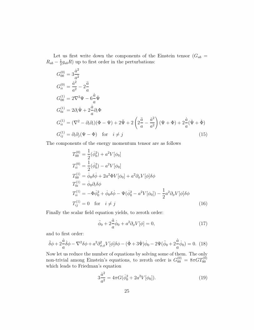
Let us first write down the components of the Einstein tensor (Gab =Rab − 1

2gabR) up to first order in the perturbations:

G(0)00 = 3

a2

a2

G(0)ii =

a2

a2− 2

a

a

G(1)00 = 2∇2Ψ− 6

a

aΨ

G(1)0i = 2∂iΨ + 2

a

a∂iΦ

G(1)ii = (∇2 − ∂i∂i)(Φ−Ψ) + 2Ψ + 2

(2a

a− a2

a2

)(Ψ + Φ) + 2

a

a(Ψ + Φ)

G(1)ij = ∂i∂j(Ψ− Φ) for i 6= j (15)

The components of the energy momentum tensor are as follows

T(0)00 =

1

2(φ2

0) + a2V [φ0]

T(0)ii =

1

2(φ2

0)− a2V [φ0]

T(1)00 = φ0δφ+ 2a2ΦV [φ0] + a2∂φV [φ]δφ

T(1)0i = φ0∂iδφ

T(1)ii = −Φφ2

0 + φ0δφ−Ψ(φ20 − a2V [φ0])−

1

2a2∂φV [φ]δφ

T(1)ij = 0 for i 6= j (16)

Finally the scalar field equation yields, to zeroth order:

φ0 + 2a

aφ0 + a2∂φV [φ] = 0, (17)

and to first order:

δφ+2a

aδφ−∇2δφ+ a2∂2φ,φV [φ]δφ− (Φ + 3Ψ)φ0− 2Ψ(φ0+2

a

aφ0) = 0. (18)

Now let us reduce the number of equations by solving some of them. The onlynon-trivial among Einstein’s equations, to zeroth order is G

(0)00 = 8πGT

(0)00

which leads to Friedman’s equation

3a2

a2= 4πG(φ2

0 + 2a2V [φ0]). (19)

25

In the linear order let us start from G(1)ij = 8πGT

(1)ij which implies Ψ = Φ.

Using the previous result, the vector constraint equations G(1)0i = 8πGT

(1)0i

imply

∂i(Ψ +a

aΨ− 4πGφ0δφ) = 0 (20)

which reduces to12

Ψ = − aaΨ+ 4πGφ0δφ. (21)

The scalar constraint equation G(1)00 = 8πGT

(1)00 becomes

2∇2Ψ− 6a

aΨ = 8πG(φ0δφ+ 2a2ΨV [φ0] + a2∂φV [φ]δφ). (22)

Now, using Einstein’s equations to express the potential

2a2V [φ0] = T(0)00 − T

(0)ii = (8πG)−1(G

(0)00 −G

(0)ii ) = (4πG)−1(

a2

a2+a

a), (23)

and substituting this result and the value of Ψ from (21) in equation (22),we obtain

∇2Ψ = 4πG(3a

aφ0δφ+ φ0δφ+ a2∂φV [φ]δφ) + (

a

a− 2

a

a

2

)Ψ. (24)

We write this equation as

∇2Ψ− µΨ = 4πG(uδφ+ φ0δφ) (25)

where µ ≡ (2 aa

2 − aa), and u ≡ 3 a

aφ0 + a2∂φV [φ], which upon use of the

expression for ∂φV [φ] from (17), gives u = aaφ0 − φ0.

Finally using the expressions for the scale factor during inflation we findµ = 0, while the slow-rolling approximation ∂2φ

∂t2= 0 corresponds in these

coordinates to the condition u = 0. Thus the last equation becomes

∇2Ψ = 4πGφ0δφ. (26)

12This, and some of the following results, follow strictly only for appropriate boundaryconditions. In later parts of the paper we will be working with Fourier decomposition ofthe various equations and the vanishing of the corresponding equations for each of theFourier mode (except the k = 0 mode) do follow independently of any considerationsinvolving boundary conditions.

26

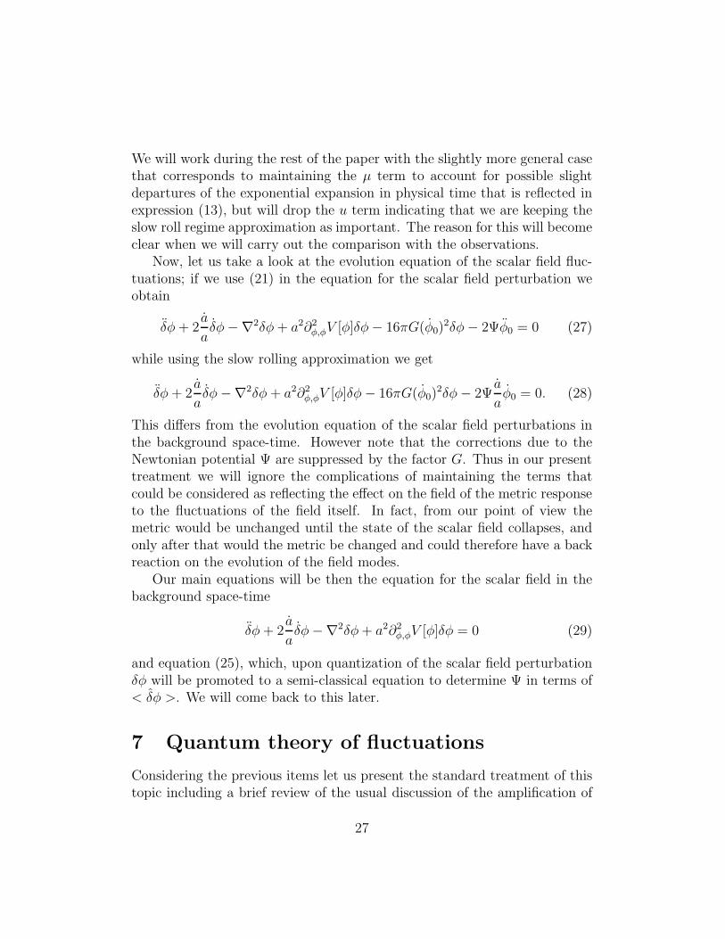
We will work during the rest of the paper with the slightly more general casethat corresponds to maintaining the µ term to account for possible slightdepartures of the exponential expansion in physical time that is reflected inexpression (13), but will drop the u term indicating that we are keeping theslow roll regime approximation as important. The reason for this will becomeclear when we will carry out the comparison with the observations.

Now, let us take a look at the evolution equation of the scalar field fluc-tuations; if we use (21) in the equation for the scalar field perturbation weobtain

δφ+ 2a

aδφ−∇2δφ+ a2∂2φ,φV [φ]δφ− 16πG(φ0)

2δφ− 2Ψφ0 = 0 (27)

while using the slow rolling approximation we get

δφ+ 2a

aδφ−∇2δφ+ a2∂2φ,φV [φ]δφ− 16πG(φ0)

2δφ− 2Ψa

aφ0 = 0. (28)

This differs from the evolution equation of the scalar field perturbations inthe background space-time. However note that the corrections due to theNewtonian potential Ψ are suppressed by the factor G. Thus in our presenttreatment we will ignore the complications of maintaining the terms thatcould be considered as reflecting the effect on the field of the metric responseto the fluctuations of the field itself. In fact, from our point of view themetric would be unchanged until the state of the scalar field collapses, andonly after that would the metric be changed and could therefore have a backreaction on the evolution of the field modes.

Our main equations will be then the equation for the scalar field in thebackground space-time

δφ+ 2a

aδφ−∇2δφ+ a2∂2φ,φV [φ]δφ = 0 (29)

and equation (25), which, upon quantization of the scalar field perturbationδφ will be promoted to a semi-classical equation to determine Ψ in terms of< δφ >. We will come back to this later.

7 Quantum theory of fluctuations

Considering the previous items let us present the standard treatment of thistopic including a brief review of the usual discussion of the amplification of

27

fluctuations by inflation. We follow in some of the discussion mainly [12] and[15].13

The starting point is the assumption is that the dynamics of the universe,during the inflationary period, is dominated by the so called inflaton field.The inflaton field is a scalar field described by the action

S[φ] =∫ [

−1

2∇aφ∇bφg

ab − V [φ]]√−gd4x. (30)

Using the form of the FRW line element the previous action becomes

S[φ] =∫ [

a2

2(−φ∂0∂0φ+ φ∂i∂jφδ

ij)− a4V [φ]

]d4x. (31)

In order for inflation to take place some hypothesis about the initial conditionfor the scalar field and its potential have to be stated. One writes the fieldas φ = φ0 + δφ, where the background field φ0 is described in a completelyclassical fashion while only the fluctuation δφ is quantized.

In these coordinates, the field equation becomes

δφ−∇2δφ+ 2a

aδφ = 0 (32)

where dots denote derivatives with respect to η and ∆ is the Laplacian onEuclidean three space (whose metric is dr2 + r2dΩ2). Note that we have ne-glected a terms proportional to ∂2φ2V [φ] using the slow rolling approximation.

If we expand the fluctuation in its Fourier components the equations ofmotion for the mode δφk becomes

δφk + 2a

aδφk − k2δφk = 0. (33)

It is well known that this equation can be further simplified by going overfrom δφ to an auxiliary field y = aδφ. In the resulting equation for y, thereis no term with a first derivative of the field anymore,

y −(∇2 +

a

a

)y = 0, (34)

13Regarding units we use a convention where the coordinates will have dimensionsof length (c = 1), a(η) is dimensionless so HI has dimensions of inverse length. Thescalar field has units of (Mass/Length)1/2 and Newton’s constant G has dimensions of(Length/Mass).

28

and in the inflationary regime with a(η) = −(HIη)−1 it can be explicitly

solved. Obviously, a quantization y of y, will immediately give a quantizationδφ = a−1y of δφ, so we will now proceed to quantize the auxiliary field y.

In order to avoid infrared problem we introduce a regularization andconsider the field in a box of side L decompose a real classical field y satisfying(34) into plane waves

y(η, ~x) =1

L3Σ~k

(ak(η)e

i~k·~x + ak(η)e−i~k·~x

), (35)

where the sum is over the wave vectors ~k satisfying kiL = 2πni for i = 1, 2, 3with ni integers. The coefficients ak(η) satisfy the equation

ak +(k2 − a

a

)ak = 0. (36)

We quantize y field imposing standard commutation relations between thefield and its canonical conjugate momentum π(y) = y−ya/a (which is equiva-lent to imposing these relations on φ and its conjugate momentum π = a2φ).Thus we write

y(η, ~x) =1

L3Σ~k

(ak(η)e

i~k·~x + a†k(η)e−i~k·~x

), where ak(η) = yk(η)ak, (37)

yk(η) is a solution of (36) and ak is the usual annihilation operator on theone particle Hilbert space H = L2(L3, d3x). Upon choosing the solutionsyk(η), y thus becomes an operator on the Fock space over H. Similarly thecanonical conjugate to y is given by

π(y)(η, ~x) =d

dηy(η, ~x)− a

ay(η, ~x) (38)

can be written as;

π(y)(η, ~x) =1

L3Σ~k,

(akgk(η)e

i~k·~x + a†kgk(η)e−i~k·~x

), (39)

where gk = yk − aayk. To complete the quantization, we have to specify the

classical solutions yk(η). This choice is not completely free: To insure thatcanonical commutation relations between y and π(y) give [ak, a

†k′] = hL3δk,k′,

they must satisfyyk(η)gk(η)− yk(η)gk(η) = −i (40)

29

for all k at some (and hence any) time η. The choice of the yk(η) correspondsto the choice of a vacuum state for the field, which in the present case, as onany non stationary space-time, is not unique. However, we must emphasizethat, at this point any such selection of a vacuum (made through the choiceof the yk(η)’s that we take as positive energy modes), would be a spatiallyhomogeneous and isotropic state of the field, as can be seen by evaluatingdirectly the action of a translation or rotation operators (associated with thehypersurfaces η = constant of the background space-time) on the state. Wewill use a rather natural candidate for such a state, the so called Bunch-Davies vacuum. It is characterized by the choice

y(±)k (η) =

1√2k

(1± i

ηk

)exp(±ikη), (41)

and

g±k (η) = ±i√k

2exp(±ikη) (42)

Note that the form of y+k reduces near η = −∞ to that of the standardpositive frequency solution in flat space. This constitutes our choice of thevacuum of the theory.14

It is convenient to rewrite the field and momentum operators in as

y(η, ~x) =1

L3

∑

~k

ei~k·~xyk(η), π(y)(η, ~x) =

1

L3

∑

~k

ei~k·~xπk(η) (43)

where yk(η) ≡ yk(η)ak + yk(η)a†−k and πk(η) ≡ gk(η)ak + gk(η)a

†−k.

Furthermore we will decompose both yk(η) and πk(η) into their real imag-inary parts yk(η) = yRk (η) + iyIk(η) and πk(η) = πR

k (η) + iπIk(η) where

yRk (η) =1√2

(yk(η)a

Rk + yk(η)a

R†k

), yIk(η) =

1√2

(yk(η)a

Ik + yk(η)a

I†k

)

(44)

πRk (η) =

1√2

(gk(η)a

Rk + gk(η)a

R†k

), πI

k(η) =1√2

(gk(η)a

Ik + gk(η)a

I†k

)

(45)where

aRk ≡ 1√2(ak + a−k), aIk ≡

−i√2(ak − a−k) (46)

14Note that the dimensions implied for ak is (Mass)1/2(Length)2 which is compatible

with the dimensionalized commutator [ak, a†k′ ] = hL3δk,k′ .

30

We note that the operators yR,Ik (η) and πR,I

k (η) are therefore hermitian op-erators. The commutation relations of the real and imaginary creation andannihilation operators are however nonstandard:

[aRk , a

R†k′

]= hL3(δk,k′ + δk,−k′),

[aIk, a

I†k′

]= hL3(δk,k′ − δk,−k′) (47)

with all other commutators vanishing. This is known to indicate that theoperators corresponding to k and −k are identical in the real case (andidentical up to a sign in the imaginary case).

8 Evolution of the fluctuations through col-

lapse

In this section, we will specify our model of collapse, and do the necessarycomputations to follow the field evolution through collapse to the end ofinflation.

The collapsing modes

To describe the collapse of the state the scalar field is in, we will use thedecomposition of the field into modes. It is imperative that these modes are‘independent’, i.e. that they give a corresponding decomposition of the fieldoperator into a sum of commuting ‘mode operators’, an orthogonal decompo-sition of the one-particle Hilbert-space, and a direct-product decompositionfor the Fock space. Furthermore, we require that the initial state of the fieldis not an entangled state with respect to this decomposition, i.e. it can bewritten as a direct product of states for the mode operators. This ensuresthat the notion of “collapse of an individual mode” will make sense.

Although the above requirements place some restrictions, there are dif-ferent possible choices for this decomposition and the corresponding choiceof modes, with possibly observable consequences. Until a less phenomeno-logical description of the collapse becomes available, we can only be guidedby simplicity, and the condition that the end result of our calculation becompatible with astrophysical observations. Throughout the main text, wewill use the modes labeled by the wave vector k and the superscript R/Iin the last section. We will however show that there is a certain degree ofrobustness of predictions under change of the mode decomposition, by re-peating the calculations that will follow below – with a different choice ofdecomposition – in appendix A.

31

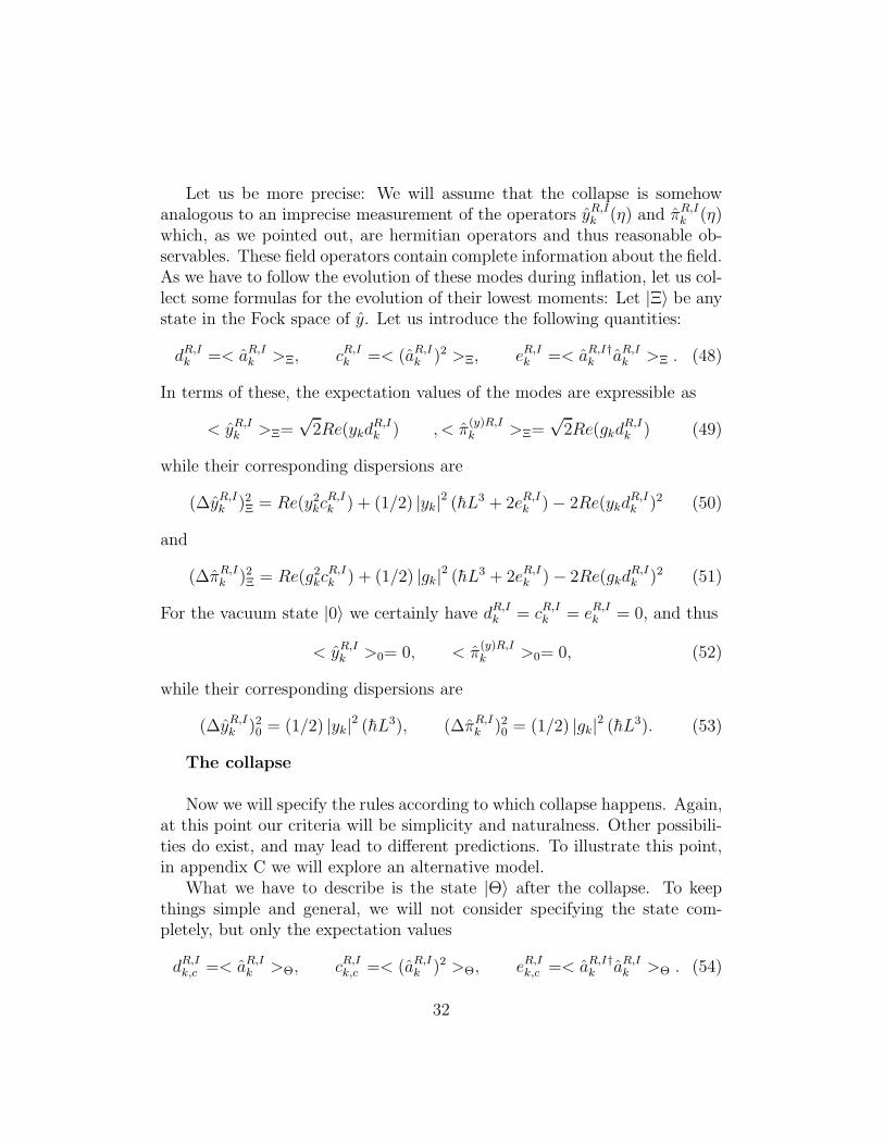
Let us be more precise: We will assume that the collapse is somehowanalogous to an imprecise measurement of the operators yR,I

k (η) and πR,Ik (η)

which, as we pointed out, are hermitian operators and thus reasonable ob-servables. These field operators contain complete information about the field.As we have to follow the evolution of these modes during inflation, let us col-lect some formulas for the evolution of their lowest moments: Let |Ξ〉 be anystate in the Fock space of y. Let us introduce the following quantities:

dR,Ik =< aR,I

k >Ξ, cR,Ik =< (aR,I

k )2 >Ξ, eR,Ik =< aR,I†

k aR,Ik >Ξ . (48)

In terms of these, the expectation values of the modes are expressible as

< yR,Ik >Ξ=

√2Re(ykd

R,Ik ) , < π

(y)R,Ik >Ξ=

√2Re(gkd

R,Ik ) (49)

while their corresponding dispersions are

(∆yR,Ik )2Ξ = Re(y2kc

R,Ik ) + (1/2) |yk|2 (hL3 + 2eR,I

k )− 2Re(ykdR,Ik )2 (50)

and

(∆πR,Ik )2Ξ = Re(g2kc

R,Ik ) + (1/2) |gk|2 (hL3 + 2eR,I

k )− 2Re(gkdR,Ik )2 (51)

For the vacuum state |0〉 we certainly have dR,Ik = cR,I

k = eR,Ik = 0, and thus

< yR,Ik >0= 0, < π

(y)R,Ik >0= 0, (52)

while their corresponding dispersions are

(∆yR,Ik )20 = (1/2) |yk|2 (hL3), (∆πR,I

k )20 = (1/2) |gk|2 (hL3). (53)

The collapse

Now we will specify the rules according to which collapse happens. Again,at this point our criteria will be simplicity and naturalness. Other possibili-ties do exist, and may lead to different predictions. To illustrate this point,in appendix C we will explore an alternative model.

What we have to describe is the state |Θ〉 after the collapse. To keepthings simple and general, we will not consider specifying the state com-pletely, but only the expectation values

dR,Ik,c =< aR,I

k >Θ, cR,Ik,c =< (aR,I

k )2 >Θ, eR,Ik,c =< aR,I†

k aR,Ik >Θ . (54)

32

where the subscript c indicates that we are talking about the post collapsevalues, to distinguish them from their pre collapse values that as we said arezero. We will drop that subscript in the following.

At this point a few remarks on our statistical treatment are in order. Weview the collapsed state of the field corresponding to our universe to be asingle state |Θ〉 and not in any way an ensemble of states. This would seem toresult in a difficulty in principle for the attempts to apply statistical analysisin our situation, and it reflects a previously mentioned difficulty of principlethat arises when dealing with the fact that we need a quantum treatment butwe have just one universe at our disposal. However it is an issue we must faceif we want to have a clear and realistic understanding of the issues at hand.The way we address this issue is related to the fortunate situation that we donot measure directly and separately the modes with specific values of ~k, butrather an aggregate contribution of all such modes to the spherical harmonicdecomposition of the temperature fluctuations on the celestial sphere. Inorder to proceed we construct an imaginary ensemble of universes. Thus wehave an ensemble of universes characterized by the after collapse state |Θ〉iwhere the label i identifies the specific element in the ensemble . Then wewill have an independent random series of numbers q

(i)~k

pertaining to valueof physical quantities in the collapsed state in each element i in the ensemblefor every single ~k (we will be assuming there are no correlations among thevarious harmonic oscillators). Our universe however, corresponds to a single

element i0 in the ensemble, leading to the choice for each ~k of a numberq(i0)~k

from among those random sequences. The point is that the complete

sequence that corresponds to our universe – i.e. the sequence q(i0)~k

of specific

quantities for fixed i0 but for the full set of ~k – will, as a result, also be arandom sequence.

In our specific calculation this approach will be taken with respect tothe quantities cck, d

ck, e

ck after considering the issues of relative overall normal-

ization of the random sequences. In fact in this first treatment we will notconcern ourselves with the quantities cck, e

ck which are related to the spread of

the wave packet after collapse, as this will be the subject of future research.Thus we focus on specifying dck: In the vacuum state, yk and π

(y)k individ-

ually are distributed according to Gaussian distributions centered at 0 withspread (∆yk)

20 and (∆π

(y)k )20 respectively. However, since they are mutually

non-commuting, their distributions are certainly not independent. In ourcollapse model, we do not want to distinguish one over the other, so we will

33

ignore the non-commutativity and make the following assumption about the(distribution of) state(s) |Θ〉 after collapse:

< yR,Ik (ηck) >Θ= XR,I

k,1 , < π(y)R,Ik (ηck) >Θ= XR,I

k,2 (55)

where XR,Ik,1 , X

R,Ik,2 are random variables, distributed according to a Gaussian

distribution centered at zero with spread (∆yR,Ik )20, (∆π

(y)R,Ik )20, respectively.

Another way to express this is

< yR,Ik (ηck) >Θ = xR,I

k,1

√(∆yR,I

k )20 = xR,Ik,1 |yk(ηck)|

√hL3/2, (56)

< π(y)R,Ik (ηck) >Θ = xR,I

k,2

√(∆π

(y)R,Ik )20 = xR,I

k,2 |gk(ηck)|√hL3/2, (57)

where xk,1, xk,2 are now distributed according to a Gaussian distribution cen-tered at zero with spread one.

We now take these equations and solve for dR,Ik . Defining the angles

α, β, γ as αR,Ik = arg(dR,I

k ),βk = arg(yk), γk = arg(gk), where the last tworefer to quantities evaluated at the collapse time ηck, the above equations canbe written

|dR,Ik | cos(αR,I

k + βck) =

1

2xR,Ik,1

√hL3, |dR,I

k | cos(αR,Ik + γck) =

1

2xk,2

√hL3.

(58)The general solution gives:

|dR,Ik | =

√hL3DR,I

k (59)

with

DR,Ik = (1/2)

(1 + z2k)1/2

zk(xR,I

k,1

2+ xR,I

k,2

2 − 2xR,Ik,1 x

R,Ik,2 (1 + z2k)

−1/2)1/2 (60)

where zk ≡ kηck, and

cos(αR,Ik + zk − π/2) = xR,I

k,2 /(2DR,Ik ) (61)

In order to more fully specify the state |Θ〉 we would need also to considerthe quantities

δ(yR,I)k = (∆yR,Ik )2Θ(η

ck), δ(π(y)R,I)k = (∆π

(y)R,Ik )2Θ(η

ck) (62)

34

To specify these, and their time evolution, we would have to specify theremaining six parameters Re(cR,I

k ), Im(cR,Ik ), and eR,I

k . However, the limitedset of results that are the concern of this paper are independent of suchchoice, and we will not further discuss the higher moments of |Θ > in whatfollows.

We need to concentrate on the expectation value of the quantum operatorwhich appears in our basic formula

∇2Ψ− µΨ = sΓ (63)

(where we introduced the abbreviation s = 4πGφ0) and the quantity Γ asthe aspect of the field that acts as a source of the Newtonian potential. In a

general situation Γ = δφ + ( aa− φ0

φ0)δφ, while in the slow roll approximation

we have Γ = δφ = a−1πy. We want to say that, upon quantization, the aboveequation turns into

∇2Ψ− µΨ = s〈Γ〉. (64)

Before the collapse occurs, the expectation value on the right hand side iszero. Let us now determine what happens after the collapse: To this end,take the Fourier transform of (64) and rewrite it as

Ψk(η) =s

k2 + µ〈Γk〉Θ. (65)

Let us focus now on the slow roll approximation and compute the right handside, we note that δφ = a−1π(y) and hence

δφk =1

a√2[gk(η)(a

Rk + iaIk) + gk(η)(a

R†k + iaI†k )] (66)

For the expectation value we find

〈Γk〉Θ =

√hL3

a√2[gk(η)(D

Rk e

iαRk + iDR

k eiαI

k)

+ gk(η)(DRk e

−iαRk + iDR,I

k e−iαIk)] (67)

=√hL3k

1

2a×

(DR

k cos(αRk + kη − π/2) + iDI

k cos(αIk + kη − π/2)

)(68)

=:√hL3k

1

2aF (k). (69)

35

We note that we can write

cos(αk + kη − π/2) = cos(αk + γck +∆k) (70)

where ∆k = k(η− ηck) = kη− zk. Then, using the expressions (58), and aftera longer calculation, we find

F (k) = (1/2)[Ak(xRk,1 + ixIk,1) +Bk(x

Rk,2 + ixIk,2)] (71)

where

Ak =

√1 + z2k

zksin(∆k); Bk = cos(∆k) + (1/zk) sin(∆k). (72)

9 Recovering the observational quantities.

Now we must compare with the experimental results. We will only do thisto a certain approximation since we will disregard the changes to dynamicsthat happen after reheating due to the transition to standard (radiationdominated) evolution.

A crucial observation for what follows is to recognize the fact that we cannot measure Ψk for each individual value of k. What we measure in fact isthe “Newtonian potential” on the surface of last scattering: Ψ(ηD, ~xD) whichis a function of the coordinates on the celestial two-sphere, i.e a function oftwo angles. From this we extract

αlm =∫

Ψ(ηD, ~xD)Y∗lmd

2Ω (73)

In fact the quantity that is measured is ∆TT(θ, ϕ) which is expressed as∑

lm αlmYl,m(θ, ϕ). The angular variations of the temperature is then iden-tified with the corresponding variations in the “Newtonian Potential” Ψ, bythe understanding that they are the result of gravitational red-shift in the

CMB photon frequency ν so δTT

= δνν

=δ(√g00)√g00

≈ δΨ. Thus we identify

the theoretical expectation αlm with the observed quantity αobslm The quan-

tity that is presented as the result of observations is OBl = l(l + 1)Cl whereCl = (2l + 1)−1∑

m |αobslm |2. The observations indicate that (ignoring the

acoustic oscillations, which is anyway an aspect that is not being considered

36

in this work) the quantity OBl is essentially independent of l, and this is in-terpreted as a reflection of the “scale invariance” of the primordial spectrumof fluctuations.

To evaluate the quantity of interest we use (65) and (69) to write

Ψ(η, ~x) =∑

~k

sU(k)

k2 + µ

√hk

L3

1

2aF (~k)ei

~k·~x, (74)

where we have added the factor U(k) to represent the aspects of the evolutionof the quantity of interest associated with the physics of period from reheat-ing to decoupling, which includes among others the acoustic oscillations ofthe plasma. It is in this expression that the justification for the use of statis-tics becomes clear. The quantity we are in fact considering is the result ofan ensemble of harmonic oscillators each one contributing with a complexnumber to the sum, leading to what is in effect a 2 dimensional randomwalk whose total displacement corresponds to the observational quantity. Toproceed further we must evaluate the most likely value for such total dis-placement. This we do with the help of the imaginary ensemble of universes,and the identification of the most likely value with the ensemble mean value.These two quantities are reasonably close in normal circumstances, where theprobability distribution has a single local maximum (the global maximum),and is not pathological in some other respect. Let us see how does this workin detail:

Using ~x = RD(sin(θ) sin(ϕ), sin(θ) cos(ϕ), cos(θ)) and standard resultsconnecting Fourier and spherical expansions we obtain

αlm = s

√h

L3

1

2a

∑

~k

U(k)√k

k2 + µ

∫F (~k)ei

~k·~xYlm(θ, ϕ)d2Ω (75)

= s

√h

L3

1

2a

∑

~k

U(k)√k

k2 + µF (~k)4πiljl((|~k|RD)Ylm(k) (76)

where k indicates the direction of the vector ~k. Now we compute the expectedmagnitude of this quantity. As a first step we take the square of the quantityof interest:

|αlm|2 = s24π2h

L3

1

a2∑

~k,~k′

U(k)√k

k2 + µ

U(k′)√k′

k′2 + µF (~k)F (~k′)jl(kRD)jl(k

′RD)Ylm(k)Ylm(k′).

(77)

37

Now we take its ensemble mean value. The calculation of such mean valuewill be simplified due to the fact that, as usual, the average over the randomvariables will lead to an cancellation of the cross terms. In our case we find

〈F (~k)F (~k′)〉 = AkAk′(〈xRk,1xRk′,1〉+ 〈xIk,1xIk′,1〉)+ BkBk′(〈xRk,2xRk′,2〉+ 〈xIk,2xIk′,2〉) (78)

where we have made use of the independence among the four sets of randomvariables xRk,1, x

Ik,1, x

Rk,2, x

Ik,2. However we need to recall that within each set

the variables corresponding to ~k and −~k are not independent. This will bereflected by setting 〈xRk , xRk 〉 = δk,k′ + δk,−k′ and 〈xIk, xIk〉 = δk,k′ − δk,−k′ inaccordance with the discussion below equation (47). Thus

〈F (~k)F (~k′)〉 = (A2k +B2

k)δk,k′ (79)

Thus we arrive to the expression for the ensemble mean value which as wesaid we will consider as a good approximation of the most likely (M.L.) value:

|αlm|2M.L. = s24π2h

L3

1

a2∑

~k

(A2k +B2

k)U(k)2k

(k2 + µ)2j2l ((|~k|RD)|Ylm(k)|2 (80)

Now we write the sum as an integral by noting that the allowed values of thecomponents of ~k are separated by ∆ki = 2π/L, thus

|αlm|2M.L. =s24π2h

a2L3(L/2π)3

∑

~k

(A2k +B2

k)kU(k)2

(k2 + µ)2j2l ((|~k|RD)|Ylm(k)|2(∆ki)3

(81)

=s2h

2πa2

∫ U(k)2C(k)k

(k2 + µ)2j2l ((|~k|RD)|Ylm(k)|2d3k (82)

where C(k) = A2k +B2

k is in fact a function of k, zk, and η.

=s2h

2πa2

∫U(k)2C(k)

(k2 + µ)2j2l ((|~k|RD)k

3dk (83)

where in the last equation we have made use of the normalization of thespherical harmonics. The last expression can be made more useful by chang-ing the variables of integration to x = kRD leading to

|αlm|2M.L. =s2h

2πa2

∫U(x/RD)

2C(x/RD)

(x2 + µR2D)

2j2l (x)x

3dx (84)

38

In the exponential expansion regime where µ vanishes, and in the limit zk →−∞ where C = 1, and taking for simplicity U(k) = U0 to be independent ofk, (neglecting for instance the physics that gives rise to the acoustic peaks),we find:

|αlm|2M.L. =s2U2

0 h

2πa2I1(l) (85)

where In(l) =∫x−nj2l (x)dx. For n = 1 we have I1(l) =

πl(l+1)

so

|αlm|2M.L. =s2U2

0 h

2a21

l(l + 1). (86)

Now, since this does not depend on m it is clear that the expectation ofCl = (2l + 1)−1∑

m |αlm|2 is just |αlm|2 and thus the observational quantity

OBl = l(l + 1)Cl =s2U2

0 h

2a2independent of l and in agreement with the scale

invariant spectrum obtained in ordinary treatments and in the observationalstudies. Now let us look at the predicted value for the observational quantityOBl. Using the expression s = 4πGφ0, the equation of motion for the scalarfield in the background in the slow roll approximation (φ = −a3

3aV ′ where

V ′ = ∂V∂φ

), and the first of Einstein’s equations, in the background which

gives 3(a)2 = 8πGa4V (φ0), we find,

OBl = (π/6)Gh(V ′)2

VU20 = (π/3)ǫ(V/M4

P l)U20 (87)

where in the last equality we have used the standard definition of the slowroll parameter ǫ = (1/2)M2

P l(V′/V )2, and Gh =M−2

P l . Note that if one couldavoid U from becoming too large during reheating, which is another aspectof the problem where the complications of the relevant physics might leaveroom for a departure from the standard results, the quantity of interest wouldbe proportional to the small number ǫ, a possibility that is not discussed inthe standard treatments, so in this case we could get rid of the ”fine tuningproblem” for the inflationary potential (i.e. even if V ∼M4

P l, the temperaturefluctuations in the CMB would be expected to be small).

Furthermore we note, as can be seen from inspection of (84), that if theevolution of the scale factor deviates slightly from the one given in (13) insuch a way that µ > 0, the effect would be to decrease the value of OBl

relative to the standard prediction of the scale invariant spectrum, for the

39

small values of l. Such effect15 has been reported [6], as we mentioned in theintroduction, and has been the subject of quite some interest lately. Moredetails about these data can be found in [1]. Moreover we note that by adetailed analysis of this sort, one could in principle extract information aboutthe deviations form the standard exponential expansion normally associatedwith inflation from the observational data.

Now let us focus on the effect of the finite value of time of collapse ηck,that is we consider the general functional form of C(k):

C(k) = 1 + (2/z2k) sin(∆k)2 + (1/zk) sin(2∆k) (88)

where we recall that ∆k = kη − zk with zk = ηckk. The first thing we note isthat in order to get a reasonable spectrum there seems to be only one simpleoption: That zk is essentially independent of k – that is the time of collapseof the different modes should depend on the mode’s frequency according toηck = z/k. Recall that the standard answer would correspond to C(k) = 1.This can be obtained here in the limit of very early collapsezk → −∞, or ifone takes the time of collapse equal to the moment of observation16. Suchpossibility will not be considered further at this point. In the case of a finitevalue for the time of collapse what we seek is for C(k) to be independentof k. In such case, the collapse would need be associated with a mechanismthat affects each mode at the appropriate time. This is a remarkable con-clusion which provides relevant information about whatever the mechanismof collapse is. This is however not enough to ensure that the resultingspectrum coincides exactly with the one obtained in the observations. Forthat we need to ensure that the other relevant parameter ηk does not in-troduce a significant k dependence. However in this case η which refers tothe conformal observation time (the time at which the observed photons areemitted, corresponding in the realistic case to the time of decoupling), is of

15It is however important to recall that, as we have indicated, all that can be extractedfrom the theory is an estimate of the “most likely” value” of αlm, as it results from a sortof random walk of the individual collapses. What is more, the likelihood of a deviationhas to do with the number of steps – i.e. individual collapsing modes – that effectivelycontribute to the random walk. This number in turn would be depend, as can be clearlyseen in the discussion above (128) of Appendix A – on global features of the universe. Itis clear that the likelihood of a deviation grows with the lowering of the values of l.

16One possibility that seems to emerge from the analysis this far is for such single eventto occur at the time of decoupling so ∆k = 0. For a possible interpretation of this seenext section.

40

course the same for all modes. Then unless the effect of the quantity ηk be-comes negligible we will not be able to account for an exactly scale invariantspectrum.

10 Further ideas

In this section we have collected some further ideas relating to the transitionto classicality and inhomogeneity: In the following subsection we present apoint of view that is to a large extent inspired in the spirit of the ManyUniverses point of view (see Sec. 4), together with the idea that missingingredient would be provided by Quantum Gravity. In Subsection 10.2 wediscuss how a mechanism that triggers collapse based on the gravitationalinteraction energy of quantum mechanical alternatives – as envisioned byPenrose – can be incorporated within the present formalism.

10.1 A special role of gravity in the Many Universes

interpretation?

A possible view contemplates a quantum evolution all the way up to thetime of observation, today. In this view the gravitational field is all thetime related to the matter through the field equation (28) which is imposedas an operator equation (no need to any semiclassical approximation in thelinearized regime).

Consider, for an analogy, a Stern-Gerlach experiment where we have anincoming electron propagating along the x-direction in a state |y,+> (spinup in the y-direction) with the magnetic field of the apparatus oriented in thez-direction (corresponding to a specific quantum state of the apparatus). Wealso introduce an observer which is treated quantum mechanically. In thiscase, the state of the apparatus selects a preferred basis where we can describethe quantum evolution. The Schrodinger evolution of the electron-apparatus-observer quantum system is such that, after the electron goes though theapparatus, the state of the system evolves into

|ψ >= (|z,+> ⊗|x+> ⊗|obs.+>) + (|z,−> ⊗|x−> ⊗|obs.−>),

where |x±> represent the two possible trajectories (up and down) of theelectron passing through the Stern-Gerlach apparatus, and |obs.±> the as-sociated two states of the observer’s mind. The choice of this basis allows the

41

interpretation of this final state where two alternative “worlds” are describedby the state vector. In each one of these worlds the observer sees the electrongoing up or the electron going down respectively. This interpretation seemsunambiguous due to the special role of the apparatus in selecting a preferredbasis in the Hilbert space of the joint system.

If we what to interpret the result of the quantum evolution of the inflatonfield during inflation we are confronted with what seems to be a similarsituation. On the one hand, the observations of the CMB are directly relatedto the fluctuations of the geometry at the time of decoupling. Let us forthe moment assume that the analog of x± is the value of the Newtonianpotential ψ. To linearized order quantum Einstein’s equations are given bythe operator version of (28) which becomes:

∇2ψ =4πGφ0

aπ(y),

It is clear that this equation connects the eigenbasis of the Newtonian po-tential with the eigenbasis of the momentum of the scalar field. At eachinstant of time η the wave function of the Newtonian potential Ψ(ψk) of eachmode is related by the previous constraint to the (squeezed) state resultingfrom the evolution of the vacuum wave function of Ψ(π(y)) associated to thescalar field. The state of the universe is thus given by Ψ(ψk)⊗Ψ(π(y)) whichcan be written as a linear superposition of eigenstates of the Newtonian po-tential and the scalar field momentum. Due to the linearity of quantummechanics, the evolution of the full state (which is always homogeneous andisotropic) can be analyzed by evolving each component separately. Everyone of these alternatives will unitarily evolve in such a way that inhomo-geneities grow, form structure, produce galaxies, and finally observers, yetthe full state remains homogeneous and isotropic. In analogy to the Stern-Gerlach experiment we can express the final quantum state of the universeas a superposition of states with its own observers. One then takes the view,that what quantum mechanics predicts about the universe is the probabilis-tic distribution of these alternatives. We can use the above formalism tomake predictions about the inhomogeneities in our own observed world byusing definition (76) in order to estimate the most likely value of |αlm| as√< α2

lm > which also leads to (93) with C(k) = 1.Of course there are certain issues with this viewpoint:

What selects the basis? Unlike the Stern-Gerlach situation there does notseem to be an obvious physical input that would lead to a preferred basis

42

where to make the decomposition. One could take the view that the basisis the one of the eigenstates of the gravitational field. After all when weobserve the CMB we do measure ψ; therefore, as in standard situations inQM we select the basis when we decide what to measure. For example if onemeasures the spin of a particle in the z-direction one should write the statein its eigenbasis to make any prediction. This fails to address the questionof how we are there to make the measurement in the first place. Only in avery specific basis would matter evolve to form observers. It seems that herewe are again confronted to some unknown mechanism selecting this basis.Gravity plays a central role in the mechanisms that allows structure to growand produce the conditions that lead to the existence of observers. Thissuggests that the gravitational realm is perhaps the place where this newelement should be found.What are the limits to which this position can be taken? We should start bynoting that in the position exposed above the full quantum state representsa set of coexistent possibilities. First of all the separation of alternativescannot be made in a strict eigenbasis of any field as the conjugate quantitywould produce large departures from what we would call the near classicalevolution. The exact nature of the states that constitute such set of noninterfering alternatives should be provided by the new element we are call-ing upon. Furthermore this element should not prevent normal quantummechanical interference in standard situations. Some sort of threshold isneeded. Presumably at the very early stages of the evolution such thresh-old would not have been reached, and thus the situation would have beendescribed as a fully interfering quantum state, the one corresponding to thescalar field vacuum. This seems to take us back to a similar sort of scenarioas the one investigated in this paper.

10.2 A ‘Penrose mechanism’ for collapse

Penrose has for a long time advocated that the collapse of quantum mechani-cal wave functions might be a dynamical process independent of observation,and that the underlying mechanism might be related to gravitational inter-action. More precisely, according to this suggestion, collapse into one of twoquantum mechanical alternatives would take place when the gravitationalinteraction energy between the alternatives exceeds a certain threshold. Infact, much of the initial motivation for the present work came from Penrose’sideas and his questions regarding the quantum history of the universe.

43

A very naive realization of Penrose’s ideas in the present setting could beobtained as follows: Each mode would collapse by the action of the gravita-tional interaction between its own possible realization. In our case one couldestimate the interaction energy EI(k, η) by considering two representativesof the possible collapsed states on opposite sides of the Gaussian associatedwith the vacuum. Let us interpret Ψ literally as the Newtonian potential andconsequently the right hand side of equation (26) as the associated matterdensity. Then we would have

EI(η) =∫

Ψ(1)(x, η)ρ(2)(x, η)dV = a3∫Ψ(1)(x, η)ρ(2)(x, η)d3x (89)

which when applied to a single mode becomes:

E(η) = (a3/L6)Ψ(1)k (η)ρ

(2)k (η)

∫d3x = (a3/L3)Ψ

(1)k (η)ρ

(2)k (η) (90)

where (1), (2) refer to the two different realizations chosen, and ρk = φ0Γk,Ψk = (s/k2)Γk, where Γk = πy

k/a and s = 4πGφ0. From equation (53) weget | < Γk > |2 = hkL3(1/2a)2. Then

EI(k, η) = (π/4)(a/k)hG(φ0)2. (91)

In accordance to Penrose’s ideas the collapse would take place when thisenergy reaches the ‘one-graviton’ level, namely when

EI(k, η) =Mp,

where Mp is the Planck mass. Using equations (65) and (53) one gets

zk =πhGφ2

0

HIMp. (92)

So zk is independent of k which according to equation (88) leads to a roughlyscale invariant spectrum of fluctuations in accordance with observations.

A more detailed exposition of this scenario and its ramifications is howeverbeyond the scope of the present paper and will be taken up elsewhere.

11 Discussion

We have discussed the problematic part of the standard analysis that issupposed to predict the primordial spectrum of fluctuations responsible for

44

the deviation of our universe from perfect homogeneity and isotropy and inparticular for the eventual evolution of galaxies, stars, and our own. Wehave argued that there is an essential element that is missing in existingproposals. We have argued that the missing element must contain somenew physics. We have considered this issue following the line of thoughtexposed by Penrose, that such new physics might be tied to some quantumaspect of gravitation, and we have employed this idea in what we calledthe collapse hypothesis, which is reflected concretely in our model in thefact that we take the Newtonian potential to couple to expectation values ofthe quantum matter degrees of freedom, and have allowed such expectationvalues to “jump” in association with the collapse process in a particular setof states. It should thus be emphasized that this can be justified only if wedeclare that gravitation is, at the quantum level, profoundly different fromother degrees of freedom as only such posture would justify the differenttreatment awarded to the gravitational and the scalar sectors in the presentwork. We have shown that a relatively simple proposal concerning a collapseof the wave function induced by some unknown mechanism, possibly tied toQuantum Gravity, can account in a transparent way for the scale invariantspectrum that seems to fit very well with the observations.

In Appendix A we have shown a degree of robustness of our approach byredoing the analysis starting from the onset with a spherical mode expan-sion of fields, and assuming that the collapse directly affects these sphericalmodes. This fact is not entirely trivial, because as we have argued before,the outcome of a collapse is associated with the quantity that is selected bythe “measurement”. Thus the exact nature of the ensemble of collapsed har-monic oscillators that constitute our field depends on the modes one choosesto define the collapsed state. However the specific statistical properties ofthe ensemble that one is examining turn out to be the same in the two situa-tions that we have considered. It is not unnatural to expect this result to begeneric if one thinks of it in analogy with an EPR type of situation: The sta-tistical properties determined by an experimentalist on one end of the set upare independent of the axis of collapse selected by the choice of polarizationused by the experimentalist in the other end, whose measurements could bethought to trigger the collapse in that case. However in our situation thepossibility of some differences in other more subtle statistical aspects of theensemble can not be so easily ruled out as we do have access to the systemon which the measurements must have occurred (i.e. in contrast with thestandard considerations for an experimentalist on one end of the EPR setup,

45

we are not denied, in principle, access to regions of the universe that mightcontain relevant information about correlations). Note on the other handthat access to such correlations might be ruled out using arguments similarto those employed by Peres to conclude that one can not experimentally de-termine the quantum state of a single photon, if one does not have accessto the information of how it was prepared [34]. One place differences canconceivably arise is in the correlations among the αlm for different m andfixed l. These issues are of course in need of further investigation.

Furthermore we have shown that, in this scheme, the resulting amplitudefor the fluctuations could become naturally small provided the physics atand after reheating does not introduce unwanted amplifications, a possibilitythat could not be easily uncovered in the standard treatments, probably dueto the fact that they do not allow for a transparent picture of the time atwhich the departure from homogeneity and isotropy starts, and is subjectedto different physical regimes of evolution. Thus our proposal opens the doorfor a study dedicated to eliminating the extreme fine tuning that is neces-sary in previous treatments. Given that our motivation had nothing to dowith this quantitative issues we view this result as another indicative of thepromising value of our approach. Furthermore we have indicated how a smalldeparture from the exponential expansion usually associated with inflationcould explain the observed decrease in the amplitude of fluctuations on largeangular scales.

It is clear the scheme is in principle susceptible to experimental exploration

as is shown by the non trivial form of the function C(k) ( equation (88)) whichcontains information about the collapse times and modes, and which is aninput to equation (84), which gives the quantities that are to be comparedwith experiment. In particular in appendix C we show explicitly that a smallchange in the collapse scheme leads to differences in the form of this function.Recall that the “standard answer” would correspond to C ≡ 1, a result thatis not trivial to obtain in this scheme as discussed in the end of section 9.

In addition our treatment reveals the various different statistical aspectsthat are at hand: First there is the statistical averaging over the modes k thatcontributes to a specific alm. Then one has the statistics that is associatedwith their average over m which leads to the observational quantity Cl orOBl in terms of which the experimental results are often exhibited. Thisclear disentanglement opens the door for more elaborated statistical analysisof the data. In particular we note that the disappearance of all informationconcerning the size of the sphere of last scattering and the effective region of

46

the universe that contains the modes that contribute to the observations isparticular to the examined values of the angular momentum and to the slowrole approximation. That is, the cancellations of the quantities RD, and L,from our final results would not occur if either we do not neglect the termsproportional to µ in (84), or if we consider small deviations from slow rollapproximation. This would lead to the appearance of δφ in (65), and thusthe source term Γ for the Newtonian potential Ψ would contain not only theterm proportional to

√k that comes from gk(η) but also terms proportional

to k−1/2 and k−3/2 coming from yk(η). This would result in the appearanceof different powers of k in equations (69), (74), (76), and (83) which wouldlead to a scale dependent contribution to the spectrum. If the observationscould be improved substantially it might be possible to see these effects.One potential source of information in this respect is in some sense alreadyavailable: One could look at the observed values of the different αlm for eachfixed value of l instead of concentrating in their average Cl and thus extractfrom the scatter in these quantities information about the effective numberof steps in the two dimensional random walks, that is the effective numberof ~k’s that contribute to their value. This in turn would provide informationabout the “effective size of the Universe”.

Finally we acknowledge we have said almost nothing about the physicalprocess that triggers the collapse of the wave function (except the exampleconsidered briefly in section 10.2 that we take at this point to be a simpleillustrative model). We have done this consciously because our aim in thiswork was to point out the difficulties with the standard views on the issue,and to illustrate the kind of effect we need the new physics to bring about.It is clear for instance, that during the collapse process the semi-classicalEinstein equations (10) can not be satisfied. We have in mind however thatthis is some approximation to a more complete description including termstied to quantum gravity and to the mechanism that triggers the collapse.Instead of equation (10), we would be considering

Gab +Qab = 8πG < Tab >, (93)

where Qab represents the back reaction of the geometry to the changes ofthe expectation values of the energy momentum tensor associated with thecollapse of the quantum state of the field. This mechanism must thereforebe such that the manipulation made within the semi-classical treatment ofEinstein’s gravity would be justified, except when the collapse takes place,the points at which the new terms would become important. In other words

47

we need Einstein’s equation to be modified by a term, that reflects the mech-anism of collapse and that is responsible for important changes only duringthe collapse itself. It is our hope that the examination of this and the otherrequirements we have found so far for the collapse mechanism would be use-ful guides in constructing specific models of the new physics behind it. Weshould stress again that our ideas in this regard are strongly influenced byPenrose’s proposals that some unknown aspect of Quantum Gravity mightbe at play. We have briefly considered one simple example of these ideas in10.2, and clearly much more detailed analysis of these issues is required. Inthis regard, and following a different line of thought, it is worth pointing outthat the quantum uncertainties in the sources of the Newtonian potentialcould be thought as inducing the kind of quantum superposition of differentgeometries that Penrose associates with the mechanism that triggers the col-lapse. In this context we note that the quantum uncertainty in δφ –which isthe one that leads to observed spectrum – behaves as 1/a while the quantumuncertainty in δφ decreases at a much slower rate. The volume over whichthese uncertainties would in principle affect the Newtonian Potential growsas a3 so their effect would in principle grow with the universe’s size, and thusin the spirit of Penrose’s ideas, the universe would, as it evolves, be approach-ing from below the threshold where the superposition of geometries wouldlead to a spontaneous collapse of the wave function. On the other hand wepoint out that δφ disappeared in our treatment as a source of the Newtonianpotential due to the slow roll approximation. Thus, one might be tempted tothink that higher order perturbative gravitational effects associated with thelatter could be the trigger, in the spirit of Penrose’s ideas, of the quantumgravitationally induced collapse. These issues will be the subject of furtherinvestigations.

We end by noting a paradoxical aspect of the situation in our field ofstudy: On the one hand there is an almost frenetic search for any form ofexperimental manifestations of any conceivable aspect of quantum gravity,while on the other hand, when faced with as clear an arena for these studies,as the one we have treated in this work, the prevailing attitude seems to beto hide the mysteries under the rug and declare that everything is fine. It isour hope that this paper contributes to changing this situation.

48

Acknowledgments

We gratefully acknowledge very useful discussions with Roger Penrose, AbhayAshtekar, James Bjorken, Carlo Rovelli, Michael Reisenberger.

This work was supported in part by DGAPA-UNAM IN108103 and CONA-CyT 43914-F grants, by NSF grant PHY-00-90091, and by the Eberly re-search funds of Penn State. HS gratefully acknowledges funding by the Max-Planck Society through the MPI for Gravitational Physics.

Appendix

A Spherical expansion

The symmetry of the situation and the physical application makes it morenatural to use spherical coordinates on the spatial slices, and spherical har-monics as a basis for the one particle space. We start again with the equationsfor the field y = aδφ,

y −(∇2 +

a

a

)y = 0, (94)

where we now write the Laplacian on Euclidean three space as

∇2φ = r−2∂r(r2∂rφ)− r−2J2φ, (95)

where J stands for the angular momentum differential operator. In order toquantize the auxiliary field y, we consider now the field in a spherical boxof radius R and require the field to vanish at its boundary. The standardseparation of variables leads us to write the field in terms of the modes

Uklm = yk(η)fkl(r)Ylm(θϕ) (96)

where the Ylm are the standard spherical harmonics and where the combina-tion fkl(r)Ylm(θϕ) are eigenmodes of the Laplacian with eigenvalue −k2. Inparticular we have fkl = ckljl(kr), where jl are the spherical Bessel functions,and the normalization is such that

∫ R

0r2dr

∫dΩ|fkl(r)Ylm(θϕ)|2 = 1. (97)

That is ckl = k3/2[∫ x(l)

i

0 (xjl(x))2)dx]−1/2 where x

(l)i corresponds to the ith zero

of jl(x), and where the allowed values of k for a given l are those that satisfy

49

kR = x(l)i . The yk(η) have to satisfy the same equation as before, and thus

we can quantize the field y as

y(η, r, θ, ϕ) =∑

k,l,m

[ak,l,myk(η)fkl(r)Ylm(θϕ) + a†k,l,myk(η)fkl(r)Ylm(θϕ)

],

(98)where the sum is over the allowed values of k for each l and as usual m ∈−l, ..., l, and we have again chosen the positive frequency solutions givenby (41) for the yk. The canonical conjugate to y can be written in a similarfashion, with gk taking the place of yk. The standard commutation relationsare equivalent to

[ak,l,m, a†k′,l′,m′ ] = hδk,k′δl,l′δm,m′ . (99)

Our definition of the components of a function F in terms of the sphericalharmonics will be Fk,l,m :=

∫d3x(fklYlm)

∗F . For the field modes we find

yk,l,m(η) = yk(η)ak,l,m + yk(η)a†k,l,−m, (100)

and express their real and imaginary parts as

yk,l,m(η)R := (1/2)[yk,l,m(η)+yk,l,m(η)

†] =1√2[yk(η)a

Rk,l,m+yk(η)a

R†k,l,m] (101)

yk,l,m(η)I := (1/2i)[yk,l,m(η) + yk,l,m(η)

†] =−i√2[yk(η)a

Ik,l,m − yk(η)a

I†k,l,m].

(102)The real and imaginary components of the annihilation operators are definedby

aRk,l,m :=1√2[ak,l,m + ak,l,m] a

Ik,l,m :=

−i√2[ak,l,m − ak,l,m] (103)

and conjugation. Consequently

[aRk,l,m, aR†k′,l′,m′] = hδk,k′δl,l′(δm,m′ + δm,m′) (104)

[aIk,l,m, aI†k′,l′,m′ ] = hδk,k′δl,l′(δm,m′ − δm,m′) (105)

[aRk,l,m, aI†k′,l′,m′] = [aIk,l,m, a

R†k′,l′,m′] = 0. (106)

The modes of π(y) can be decomposed in the same way. The only thing thatchanges in comparison to (101,102) is that yk gets replaced by gk. Now weconsider the quantity of interest that is determined by the following quantity,

dR,Ik,l,m =< aR,I

k,l,m >Θ:=√hDR,I

k,l,meiαR,I

k,l,m (107)

50

These quantities which as before associated with the collapsed state expec-tation value of the field and momentum, which in our model for the collapseare determined by the relation at the time of collapse

< yR,Ik,l,m(η

ck) >Θ = xR,I

k,l,m,1

√(∆yR,I

k,l,m)20 = xR,I

k,l,m,1|yk(ηck)|√h/2, (108)

< π(y)R,Ik,l,m (ηck) >Θ = xR,I

k,l,m,2

√(∆π

(y)R,Ik,l,m )20 = xR,I

k,l,m,2|gk(ηck)|√h/2, (109)

where as before we have for any time at or after the collapse,

< yR,Ik,l,m(ηk) >Θ =

√2ℜ(yk(ηk)dR,I

k,l,m), (110)

< π(y)R,Ik,l,m (ηck) >Θ =

√2ℜ(gk(ηk)dR,I

k,l,m) (111)

Again in terms of the phases βk = arg(yk), γk = arg(gk), where the last tworefer to quantities evaluated at the collapse time ηck, the above equations canbe written

DR,Ik,l,m cos(αR,I

k +βck) =

1

2xR,Ik,l,m,1, DR,I

k,l,m cos(αR,Ik + γck) =

1

2xR,Ik,l,m,2. (112)

To connect to observations, we again use the relation ∇2Ψ − µΨ = sΓ.Decomposing both sides into spherical harmonics, we find

Ψklm(η) = − sU(k)

(k2 + µ)Γklm(η) (113)

where, once more, the factor U(k) accounts for the physical evolution fromreheating to decoupling. The right hand side is connected to the scalar fieldvia, Γ = 1

aπ, so in our context

Γk,l,m(η) =1

a< π

(y)k,l,m(η) >Θ . (114)

The observational quantity αlm can be expressed as

αlm =∫

Ψ(ηD, ~xD)Y∗lmd

2Ω =∑

k

Ψklm(ηD)fkl(RD). (115)

Again we see that this quantity is a sum of the complex quantities associatedwith the collapse and thus can be viewed as a two dimensional random walkwith variable step size. We resort once more to the mathematical trick of

51

identifying the most likely value of the this magnitude with the mean value ofan ensemble of identical instances. This corresponds to identifying the mostlikely value of the total displacement of the random walk with its ensembleaverage. Thus we write

|αlm|2MostLikely =<< |αlm|2 >>=<< |∑

k

Ψklm(ηD)|2 >>, (116)

=∑

k,k′

s2U(k)U(k′)

(k2 + µ)(k′2 + µ)<< Γklm(ηD)Γk′lm(ηD) >> fkl(RD)fk′l(RD) (117)

Now we evaluate this ensemble average noting that

Γklm(η) = (1/a)< π(y)Ik,l,m(η) >Θ +i < π

(y)Ik,l,m(η) >Θ (118)

= (√2/a)ℜ(gk(η)dRk,l,m) + iℜ(gk(η)dIk,l,m) (119)

= (√2/a)|gk(η)|

√hDR

k,l,m cos(αRk,l,m + γk) (120)

+ iDIk,l,m cos(αI

k,l,m + γk) (121)

so that writing αR,Ik,l,m+ γ = αR,I

k,l,m+ γck+∆k where ∆k = k(η− ηck), and using(112), we find

Γklm(η) = (√2/a)|gk(η)|

√h(1/2)[xRk,l,m,1

√1 + 1/z2kSin(∆k) (122)

+ xRk,l,m,2(cos(∆k) + (1/zk)Sin(∆k))] (123)

+ i[xIk,l,m,1

√1 + 1/z2kSin(∆k) (124)

+ xIk,l,m,2(cos(∆k) + (1/zk)Sin(∆k))] (125)

Thus upon taking the ensemble average, and using << xAk,l,m,NxA′

k′,m,l,N ′ >>=δk,k′δA,A′δN,N ′ (where A,A′ stand for R or I and N,N ′ stand for 1 or 2) wefind:

<< Γklm(η)Γk′lm(η) >>= δk,k′(h/2a2)|gk(η)|2C(k) (126)

with C(k) given by (88). We thus have obtained a useful expression for thedesired quantity:

<< |αlm|2 >>=∑

k

s2U(k)2

(k2 + µ)2(h/2a2)|gk(η)|2C(k)|fkl(RD)|2 (127)

Now we evaluate this sum. To proceed we recall that the sum is over thevalues of k such that kR = x

(l)i , the zeros of the function jl(x). Next we

52

write fkl(RD) = ckljl(kRD) where ckl = k3/2[∫ x(l)

i

0 (xjl(x))2)dx]−1/2. Thus

fkil(RD) = ciljl(x(l)i RD/R). Now using eq 11.170 of [35] we find

∫ x(l)i

0 (xjl(x))2)dx =

(x(l)i )3j2l+1(x

(l)i )/2. Now the approximate expression ( valid for large x) for

the spherical Bessel functions jl(x) = (1/x) sin(x − lπ/2) ( eq. 11.161a of

[35]) we see that the ith zero of jl(x) is x(l)i = (i + l/2)π, thus (jl+1(x

(l)i ) =

(x(l)i )−1 = [(i+ l/2)π]−1. Therefore ckl = k3/2[(x

(l)i )/2]−1/2 = (k

√2/R) where

in the last step we used the fact that the allowed values of ki must satisfykiR = x

(l)i . We also use the fact that |gk(η)|2 = k/2, and thus we find

<< |αlm|2 >>=∑

k

s2U(k)2

(k2 + µ)2(h/2a2)(k/2)(2k2/R)|j2l (kRD)|2C(k) (128)

which we write as

<< |αlm|2 >>=hs2

2a2R

∑

k

E(k), E(k) :=U(k)2k3

(k2 + µ)2|j2l (kRD)|2C(k).

(129)Now we use the uniform continuity of the function F , choose ǫ > 0 and findthe δ > 0 such that for |k− k′| < δ the corresponding |E(l)(k)−E(l)(k

′)| < ǫ,and then write

∑

k

E(k) = δ−1∞∑

n=0

∑

k∈[nδ,(n+1)δ]

E(l)(nδ)δ (130)

Now the number of allowed values of k = (1/R)xl)i = (i + l/2)π/R in the

interval [nδ, (n + 1)δ] is N = Rδ/π. Then we can write

∑

k

E(k) = δ−1∞∑

n=0

NE(l)(nδ)δ = (R/π)∫ ∞

0E(l)(k)dk (131)

where in the last step we have taken the limit ǫ→ 0. Thus we finally obtain,

<< |αlm|2 >> =hs2

2a2R(R/π)

∫ ∞

0E(l)(k)dk (132)

=hs2

2a2π

∫ ∞

0

U(k)2k3

(k2 + µ)2|j2l (kRD)|2C(k)dk (133)

which is the same result that was obtained in the analysis of Section 9.

53

B On the meaning of the Newtonian poten-

tial

Let us consider the space-time given by the perturbed metric:

ds2 = a(η)2[−(1 + 2Ψ)dη2 + (1− 2Ψ)δijdx

idxj]

(134)

In this space-time light will travel according to

dη = ±[(1− 2Ψ)

(1 + 2Ψ)

]1/2dx ≈ ±(1− 2Ψ)dx (135)

We want to consider light signals being emitted from the surface of lastscattering at a given ηD and arriving to us from all angular directions. Wewill assume that we and the CMB radiation emitting plasma are at rest inthe background space-time so that both we and the plasma fluid follow worldlines of fixed x.

Thus a light signal that starts at η(1)e at a given position xe and arrivesto the origin at x = 0 at η(1)o , will satisfy

η(1)o − η(1)e =∫ xe

0(1− 2Ψ)dx (136)

Consider a second signal emitted an extremely short time after the first one(we are thinking of fractions of a second), and from the given position xe atη(2)e = η(1)e + δηe and its arrival to the origin at x = 0 at η(1)o = η(1)o + δηo. Itis clear then that

η(2)o − η(2)e =∫ xe

0(1− 2Ψ)dx (137)

and therefore δηe = δηo. Now let us consider the actual proper times mea-sured by observers at rest between the two emission events δτe and betweenthe two detection events δτo. It is clear that δτ = a(η)[1 + 2Ψ](1/2)δη ≈a(η)[1 + Ψ]δη so

δτe = a(ηe)[1 + Ψe]δηe, δτo = a(ηo)[1 + Ψe]δη0 (138)

Thus we findδτoδτe

=a(ηo)

a(ηe)(1−Ψo)[1 + Ψe] (139)

where it is clear that all the angular dependence is in the factor [1+Ψe], whilea(ηo)a(ηe)

(1 + Ψo) represents the combine effect of the overall cosmic expansion

54

and the gravitational potential at our location. The quantity δτoδτe

is clearlyencoding the standard gravitational red-shift and is equal to the frequencyratio νo/νe which in turn is associated with the temperature of the observedCMB. Note that the whole angular dependence is in Ψe, so it is clear thatwhat we have been computing is indeed an observable quantity, and in thatsense it is gauge invariant.

C Alternative Collapse Scheme

Here we want to consider an additional natural possibility for the collapse.The main motivation is to explicitly show how observational data could beuse to shed light into the details of the collapse mechanism. The idea weconsider here is that as it is only the field’s momentum which acts as asource, at leading order, for the Newtonian potential, it should be only thisquantity that would be subjected to a change in the expectation value duringthe collapse. This view seems to be close in spirit to the ideas of Pen roseregarding the quantum uncertainties that the gravitational potential wouldbe inheriting from the matter fields quantum uncertainties, as fundamentalfactors triggering the collapse. In such a situation we would have a collapsedstate for which for |Θ〉 after collapse:

< yR,Ik (ηck) >Θ= 0, < π

(y)R,Ik (ηck) >Θ= XR,I

k (140)

where XR,Ik are random variables, distributed according to a Gaussian dis-

tribution centered at zero with spread (∆π(y)R,Ik )20, respectively. Thus

< π(y)R,Ik (ηck) >Θ = xR,I

k

√(∆π

(y)k )20 = xR,I

k |gk(ηck)|√hL3, (141)

where xk are now distributed according to a Gaussian distribution centeredat zero with spread one. In this situation the whole analysis of Section 9goes through, with the only difference being that now we have:

F (k) = (xRk + ixIk)[cos(∆k)− (1/zk) sin(∆k)] (142)

so that

〈F (~k)F (~k′)〉 = δk,k′[I + (1− (1/z2k)) sin2(∆k)− (1/zk) sin(2∆k)] (143)

55

And therefore

|αlm|2MostLikely =s2h

2πa2

∫U2(x/RD)C

′(x/RD)

(x2 + µR2D)

2j2l (x)x

3dx (144)

where now the function C is slightly different from the one found in thedemocratic collapse model, and is given by

C ′(k) = [1 + sin2(∆k)(1− (1/z2k))− (1/zk) sin(2∆k)] (145)

We see that in principle the observations could help distinguish between thedifferent collapse models, and therefore it is clear that the question of theexact mechanism for the origin of the primordial fluctuations is both affectedand can help shed light on a fundamental issue in our understanding ofquantum mechanics as applied to the universe as a whole.

References

[1] “Cosmological parameters From First results of Boomerang” BoomerangCollaboration (A.E. Lange et al.) Phys. Rev. D,63, 042001,(2001); G.Hinshaw et. al., Astrophys. J. Supp. , 148, 135 (2003); “Power Spec-trum of Primordial Inhomogeneity Determined from four Year COBEDMR SKY Maps”, K.M. Gorski , A.J. Banday , C.L. Bennett(NASA,Goddard), G. Hinshaw, A. Kogut , G.F. Smoot , E.L. Wright , Astro-phys. J. 464, L11, (1996); “First Year Wilkinson Micorowave AnisotropyProbe (WMAP) Observations: Preliminary Results” C.L. Bennett et al.Astrophys. J. Suppl. 148, 1,(2003); “First Year Wilkinson MicorwaveAnisotropy Probe (WMAP) Observations: Foreground Emission”, C.Bennett et al. Astrophys. J. Suppl. 148, 97,(2003).

[2] “Quantum Mechanics of the scalar field in the new inflationary Uni-verse”, A. Guth and S.-Y. Pi Phys. Rev. D 32, 1899, (1985).

[3] “Fluctuations in the Inflationary Universe”, S. W. Hawking Nucl. Phys.

B 224, 180, (1983).

[4] See for instance discussion in “The Early Universe”, E.W. Kolb andM.S. Turner, Frontiers in Physics Lecture Note Series (Addison WesleyPublishing Company 1990).

56

[5] “An Alternative to Inflation”, S. Hollands and R.M. Wald,Gen.Rel.Grav. 34, 2043,(2002) [arXive: gr-qc/0205058].

[6] “Is the Universe out of Tune”, G.D. Starkman and D. J. Schwartz,Scientific American, Vol 293, No 2, 48, (2005).

[7] “Semiclassicality and decoherence of Cosmological perturbations”, D.Polarski and A.A. Starobinsky,Class. Quant. Grav. 13, 377 (1996) [arX-ive: gr-qc/9504030]

[8] “Origin of Classical Structure From Inflation”, C. Kiefer Nucl. Phys.

Proc. Suppl. 88, 255 (2000) [arXiv:astro-ph/0006252], and referencestherein.

[9] “Space-time correlations in Inflationary Spectra”, D. del Campo, andR. Parentani, Phys. Rev. D 70, 105020 (2004) [arXiv:gr-qc/0312055]

[10] “Environment Induced Superselection In Cosmology”, W.H. Zurek, inMoscow 1990, Proceedings, Quantum gravity (QC178:S4:1990), 456-472.(see High Energy Physics Index 30 (1992) No. 624)

[11] “Decoherence Functional and Inhomogeneities in the Early Universe”,R. Laflamme and A. Matacz, Int. J. Mod. Phys. D 2, 171 (1993)[arXiv:gr-qc/9303036]

[12] “Lectures on the Theory of Cosmological Perturbations”, R.H. Bran-denberger,Lect. Notes Phys. 646, 127 (2004) [arXiv:hep-th/0306071]

[13] “Gauge Invariant Cosmological Perturbations” R. Branderberger H.Feldman and V. Mukhavov, Preprint Brown HET 845 (1992); Phys.Rep. 215, 203, (1992)

[14] “Cosmology and Astrophysics Through Problems”, T. Padmanabhan(Cambridge University Press 1996).

[15] “ Cosmological Inflation and Large Scale Structure”, A.R. Liddle andD.H. Lyth (Cambridge University Press 2000).

[16] “The self-induced approach to decoherence in cosmology,” M.Castagnino and O. Lombardi,Int. J. Theor. Phys. 42, 1281 (2003)[arXiv:quant-ph/0211163].

57

[17] “Origin of Structure in the Universe” J.J. Halliwell and S. W. Hawking,Phys. Rev. D, 31, 1777,(1985).

[18] “Inflationary Cosmological Perturbations of Quantum Mechani-cal Origin” J. Martin, Lect. Notes Phys. 669, 199 (2005)[arXiv:hep-th/0406011]; “ Best Unbiased Estimates for Microwave back-ground Anisotropies”, L.P. Grishchuk and J. Martin, Phys. Rev. D 56,1924 (1997) [arXiv:gr-qc/9702018]

[19] “The Emperor’s New Mind”, R. Penrose ( Oxford University Press1989).

[20] “Structure in the COBE DMR first year maps” G.F. Smoot et. al.,

Astrophys. J., 396, L1 (1992).

[21] S. Adler, (Princeton) Private Communication.

[22] “Nonlocality in Quantum Physics”, A. Anaoljevich Grib and W. AlvesRodrigues Jr. (Kluwer Academic / Plenum Publishers 1999).

[23] “Quantum Cosmology Problems for the 21st Century”, J. B. Hartle,arXive: gr-qc/9701022.

[24] “Generalized Quantum mechanics for Quantum Gravity”,J. B. Hartle,arXive: gr-qc/0510126.

[25] “The Reduction of the State Vector and Limitations on Measurementin Quantum Mechanics of Closed Systems, J. B. Hartle, in “Directionsin Relativity. Vol. 2: Proceedings”, B.L. Hu and T.A. Jacobson (eds.),Cambridge University Press, Cambridge, 1993. [arXive: gr-qc/9301011]

[26] “Consistent Sets Yield Contrary Inferences in Quantum Theory”, A.Kent, Phys. Rev. Lett. 78, 28749 (1997); “Comments on “ConsistentSets Yield Contrary Inferences in Quantum Theory”, R. Griffiths andJ.B. Hartle,Phys. Rev. Lett. 81, 1981 (1998) [arXiv:gr-qc/9710025]

[27] “Decoherence in Quantum Cosmology”, J.J. Halliwell, Phys. Rev. D,39, 2912,(1989)

[28] “Recent Advances in Stochastic Gravity Theory and Issues”, B. L. Huand E. Verdaguer, arXive: gr-qc/0110092.

58

[29] “Decoherence in Quantum Cosmology at the onset of Inflation”, A.O.Barvinsky, A.Y. Kamenshchik, C. Kiefer, and I.V. Mishakov, Nucl.

Phys. B 551, 374 (1999) [arXiv:gr-qc/9812043]

[30] “Speakable and Unspeakable in Quantum Mechanics”, J. S. Bell (Cam-bridge University Press 1987).

[31] “Is the Moon There when nobody Looks?” D. Mermin Physics Today

32, 38, (1985).

[32] “Experimental realization of Einstein-Podolsky-Rosen-Bohm Gedanken-experiment: A New violation of Bell’s inequalities” A. Aspect, P. Grang-ier, G. Roger, Phys. Rev. Lett. 49, 91, (1982).

[33] “A Unified Dynamics For Micro And Macro Systems”, G. C. Ghirardi,A. Rimini, and T. Weber,Phys. Rev. D 34, 470, (1986).

[34] Quantum Theory: Concepts and Methods, A. Peres (Kluwer, AcademicPublishers, 1993).

[35] Mathematical Methods for Physicists, G. Arfken, (Academic Press NewYork 1970).

[36] “Decoherence during inflation: The generation of classical inhomo-geneities,” F. C. Lombardo and D. Lopez Nacir, Phys. Rev. D 72, 063506(2005) [arXiv:gr-qc/0506051].

59