1

On the Principles/Importance of Thermodynamics

Dr. A. Özer Arnas Professor of Mechanical Engineering United States Military Academy at West Point West Point, NY 10996 Introduction

Precise thermodynamics education is a requirement to discuss issues that one faces in thermodynamics and re-sulting studies in global warming, energy conversion and other energy related topics that affect sustainability of the environment in the global sense. For this reason, learning, understanding and meaningful and relevant ap-plication of topics in thermodynamics are required. To accomplish this, educating students at the undergraduate and graduate levels in classical, statistical and non-equilibrium thermodynamics becomes important. Here a short synopsis of fundamentals of classical thermodynamics are discussed with the intent of bringing clarity to the laws of thermodynamics and their application in design of experiments, applications in other fields such as heat transfer, and physical interpretation of the mathematical relations that are so useful in explaining why cer-tain things happen in thermodynamics and nature. Nature is the ultimate customer.

For all scientist and engineers, the courses that end in –ics must be studied and understood well with their cor-rect and precise application, such as mathematics, physics, chemical kinetics, mechanics as well as ethics and economics. Of course, thermodynamics is one portion of mechanics that is very important in the education of all engineers.. It relates natural phenomena to some order and disorder. From a thermal energy point of view therefore, thermodynamics is the science that dictates what happens in nature and what not and why. Thus to better understand nature, the implications of energy usage on the environment and sustainability of what we en-joy today, we need to study precise thermodynamics.

Definitions

Definitions in thermodynamics must be precise to make everything that follows correct. Thus, in nature, there are only three types of systems. The closed system is one for which the mass within the boundaries remain a constant, such as a tank or a piston-cylinder arrangement. The filling/emptying system is the one that a tank with a valve characterizes where mass can either enter or leave the tank. Both cannot occur simultaneously. If a system has mass entering and leaving the boundaries, then it is called open. There are only eight thermodynamic properties. The measurable ones are pressure, p, volume, V, and tempera-ture, T. As a consequence of the first law of thermodynamics, internal energy, U, is introduced followed by the second law of thermodynamics and the introduction of entropy, S. Then three convenience properties are de-fined in terms of the five above: enthalpy H = U+pV, the Gibbs’ function G = H-TS, and the Helmholtz poten-tial F = U-TS. The rest should be called physical properties of a system, such as the mass m. In thermodynamics equilibrium is required to solve a problem. By definition, when two systems reach the same temperature T, they are called to be in thermal equilibrium. When they reach the same pressure p, they have mechanical equilibrium, and when they have the same electrochemical potential μi , they have chemical equilib-rium. When all three happen simultaneously, then thermodynamic equilibrium exists. One of the more important statements in thermodynamics is the state principle. This principle is important not only in thermodynamic analyses but in applied areas like heat transfer. This principle states that any two inde-pendent and intensive thermodynamic properties would define any of the others and fix a thermodynamic state and the situation is unique no matter which choice is made. A lack of understanding of this principle may lead into published work which has no meaning at all, Chawla (1978). Thus once a thermodynamic state is defined then a characteristic line that connects any two such states is called a thermodynamic process. A sequence of thermodynamic processes ending up at the initial thermodynamic state is called a thermodynamic cycle.

Conservation equations

These equations that apply may be obtained using the Reynolds’ Transport Theorem. Its use is common to all of these conservation laws and will be done systematically for each one of them. Considering at time t, Bsystem(t) = BCV(t) and at time t+Δt, Bsystem(t+Δt) = [BCV(t+Δt) + Bout – Bin] where the amount of B that exited the control

volume is given as Bout = b(mout) = b[(ρ)(V

out)(Aout)(Δt)] and Bin= b(min) = b[(ρ)(V

in)(Ain)(Δt)] is the amount of B that entered the control volume. Subtracting the first term from the second and dividing by Δt results in

t

tVbtVb

t

tBttB

t

tBttBininoutoutCVCVsystemsystem

-[(-(-( . Taking the limit of this

equation as Δt approaches 0 yields the simplified equation

ininoutoutCVsys AVAVb

dt

dB

dt

dB . Rewriting

the outflow and inflow terms for the entire control surface in this equation gives CS

CVsys dAnVbdt

dB

dt

dB

where the dot product, nV , is defined as (V n cosθ)� where θ is the angle between nV

to . The total amount

of extensive property B, (B=m b), in the control volume is determined by integrating over the entire control vol-

ume as CVCV bdB V . Upon substitution and combination, the Reynolds Transport Theorem is obtained as

CSCV

sys dAnVbbdVdt

d

dt

dB)(

where the left hand term is the time rate of change of extensive property

(B) in the system, the first term on the right hand side of the equation is the time rate of change of intensive property (b) in the control volume, and the second term on the right hand side of the equation is the net flow of intensive property (b) across the control surface. A positive value indicates net flow across the control surface is out of the control volume while a negative value indicates net flow across the control surface is into the control volume. There are two conservation equations, that of mass and energy – the first law of thermodynamics. For the case of conservation of mass,

Closed system: constant.m

Open system: ..

mmoutin

Filling system: finalin

initial mmm

Emptying system: finalout

initial mmm .

Applying the Reynolds’ Transport Theorem to the first law of thermodynamics, the result be-

comes

CV CS

system dAnVeedVdt

d

dt

dE)( . This statement is very similar to money and banking; the differ-

ence is that nature does not permit overdraw of funds, namely one cannot use what is not there, whereas the

bank just charges us money for overdraft. At steady state, therefore, dUWQ . For a cycle, WQ

resulting in the fact that 0)( propertyddU . This is a very important result which will be used later. Ap-

plication of the above theorem to various systems in nature results in the first law of thermodynamics as

Closed system: ieieie UUWQ

Open system: )2

()2

(

2

.

2

...

gzV

hmgzV

hmWQie

ieie

Filling system: 11

2

22 )2

( umgzV

hmumWQi

ieie

Emptying system: 1122

2

)2

( umumgzV

hmWQe

ieie

Sign convention in thermodynamics

We cannot overemphasize the importance of this since most, if not all, textbooks do not strictly follow the con-vention. What convention is followed is not important, the consistent use of it is. For example, Callen (1960) says that all energy in is positive and all energy out is negative, and in that text this is followed consistently whereas most commonly used undergraduate and graduate textbooks do not, as is shown in the Bibliography and References of Arnas, et al (2003). Precision is very important, as is mentioned in Obert (1960) In most textbooks, all energy transfer due to a difference of temperature only called heat, in is positive and heat out is negative, and all energy transfers due to a potential difference other than temperature called work, in is negative and work out is positive giving us HIP to WIN. In all that we will do, this convention will be followed due to its universal and more common usage. For the equivalence of heat to absolute temperature, consider a Carnot cycle, Fig.1. It is made of two reversible adiabatic lines and two constant temperature heat reservoirs. If the working fluid is considered to be an ideal gas, for simplicity of algebra, then the energy added at TH is given by, for an

ideal gas,

b

cHbc V

VT

M

mQ ln .

Figure 1. The Carnot cycle

Similarly for the process (d-a),

d

aLda V

VT

M

mQ ln ; thus the ratio becomes

b

c

d

a

H

L

bc

da

V

V

V

V

T

T

Q

Q

ln

ln

. Since the

process (a-b) is reversible and adiabatic, then [- m cv dT = p dV] =

V

dVT

M

m. This integrates to give for

process (a-b) the result of

a

b

T

T

v V

V

T

dTc

M H

L

ln . For the process (c-d), a similar results is obtained as

c

d

T

T

v V

V

T

dTc

M L

H

ln . Therefore, since the limits of integration are reversed, the equivalence

gives

c

d

b

a

V

V

V

Vlnln or {-[ln Vc – ln Vb]} = [ln Va – ln Vd] resulting in 1ln/ln

d

a

b

c

V

V

V

V . This upon sub-

stitution yields the expected result of

H

L

H

L

T

T

Q

Q. This relation permits one to substitute temperatures for

heat quantities in the determination of Carnot performance criteria which quickly give extremum values for the actual efficiencies for engines, η, as well as coefficient of performances for refrigerators, β, and heat pumps, γ. It must be remembered that one of the heat quantities is negative, out of a system, as it should be since the ratio of absolute temperatures is always positive. With reference to Arnas, et al (2003), we can examine the various

P

v

d

c

a

b

TH, isothermal

TL, isothermal

adiabatic

adiabatic

All processes are reversible

QH

-QL

details of this result particularly with respect to engine efficiency and refrigerator and heat pump coefficient of performances. For this demonstration, we will use the sign convention of Callen (1960) that all energy transfers into a system are positive and all out of the system are negative.

Performance characteristics of devices

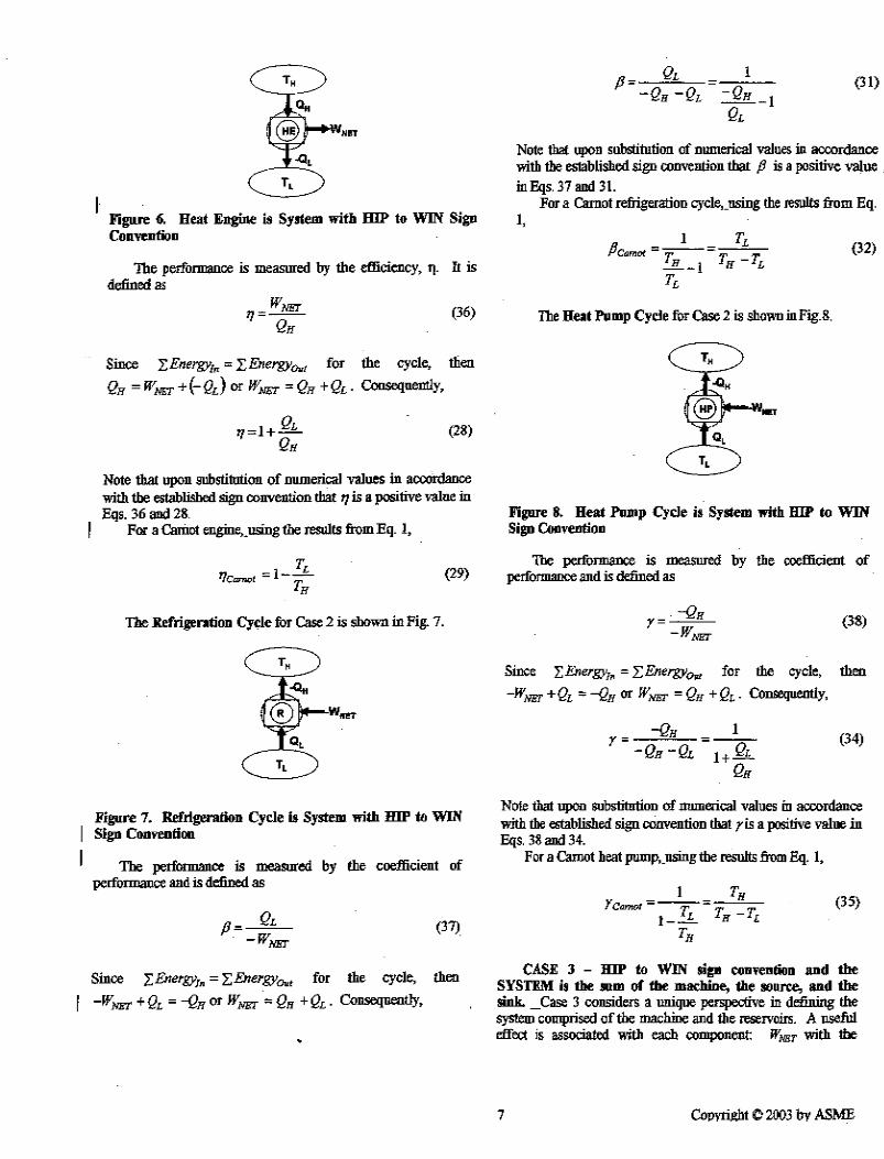
Consider a heat engine that receives energy (QH) from a reservoir at (TH) and produces work (–Wnet) while re-jecting energy (–QL) to a reservoir at (TL). Since the performance of any device is measured by the ratio of the

net useful effect to the total cost to obtain that effect, then

H

net

Q

W . Also we have outin EE giving

)( LnetH QWQ . Solving for netW and substituting into the efficiency equation, the result becomes

H

L

H

LH

Q

Q

Q

QQ1 . Using the equivalence equation, the efficiency of a Carnot engine reduces to

H

L

T

T1 .

For a refrigerator, the net effect is the cooling that we get, (QL), from a cold reservoir at (TL). The work re-quired to pump this energy is (Wnet), and the energy given off to the environment at a temperature (TH) is (-QH). Therefore, the performance parameter, coefficient of performance for a refrigerator becomes

1

1

)(

L

HLH

L

net

L

QQQQ

Q

W

Q which reduces to

LH

L

TT

T for a Carnot refrigerator.

For a heat pump, the net effect is the heating that we get, (-QH) into a reservoir at a temperature of (TH). The work required to pump this energy is (Wnet), and the energy that is taken out of the environment at a temperature (TL) is (QL). Therefore, the coefficient of performance for a heat pump becomes

H

LLH

H

net

H

Q

QQQ

Q

W

Q

1

1

)( which reduces to

LH

H

TT

T for a Carnot heat pump. It is also

easy to prove that )}1({ using the results obtained above.

Second law of thermodynamics

The second law of thermodynamics denies a system the possibility of utilizing energy in a particular or arbitrary way. There are two basic definitions of the second law which were stated at different times by different people, historically speaking.

Kelvin-Planck statement It is impossible to construct an engine which is operating in a cycle that will produce no effect other

than the extraction of energy from a reservoir and the performance of an equivalent amount of work. Thus an efficiency of 100% is not a possibility.

Clausius statement It is impossible to construct a device which while operating in a cycle will produce no effect other than

the transfer of energy from a colder to a hotter body. Thus a refrigeration unit requires energy input as work; otherwise it cannot function. These two statements are equivalent and the assumption of the validity of one leads to the situation given by the other. Consider that the Kelvin-Planck statement is valid. If now one constructs a refrigerator running with the work of the engine and extracting energy [-Qc] from the cold reservoir, then the engine-refrigerator system is one which absorbs energy from a cold reservoir and transfers it to the hot reservoir without any external work, a situation which the Clausius statement refutes. If this were possible, the energy in the oceans at a low and cold temperature could be utilized to run all kinds of equipment without any external work; an impossible situation known to all.

If now the Clausius statement is considered to be valid, then the refrigerator functions without any external work. At the same time, an engine placed between the same two reservoirs produces work. The refrigerator-

engine system leads to a situation where an amount of energy is absorbed from a hot reservoir and an equivalent amount of work is performed, a situation that the Kelvin-Planck statement refutes. If this were valid, all the fuel consumed in the engine of a car would be used in the form of work without any losses whatsoever; another im-possible situation that is well known to all. All physical systems must function in such a way as not to violate ei-ther one of these statements. Otherwise a perpetual motion machine of the second kind will result.

The CARNOT Principle

This is one of the fundamental principles of thermodynamics. It says that there is no heat engine oper-

ating between two given reservoirs that can be more efficient than a Carnot heat engine operating between the same two reservoirs. To prove this statement, assume that the reverse is true. Then since the Carnot engine is reversible, it can be reversed to operate as a refrigerator. Therefore, if the engine E is more efficient than the Carnot engine CE, the result becomes (ηE > ηCE).

Figure 2. The graphical explanation of the Kelvin-Planck and Clausius statements of the second law.

This can also be written as

CH Q

W

Q

W giving as the final result HC QQ . If this is the case, then there is a

net flow of energy in the form of heat from the cold to the hot reservoir without any consumption of work or other external effects. Such a result is impossible since it leads to the contradiction of the Clausius statement of the second law of thermodynamics. Thus the original assumption was wrong which says that the efficiency of an engine cannot be larger than that of a Carnot engine operating between the same two reservoirs. A corollary to the Carnot principle is that all Carnot engines operating between the same two temperature reservoirs TH and TL have the same efficiency. The proof of this statement follows from the above. Assume that the first one is more efficient than the other. A contradiction will be observed. Then assume the other way around. The same contradiction will be obtained. The only possibility remaining, therefore, is naturally the equivalence of the two efficiencies. Entropy

Entropy is a thermodynamic property which comes about as a result of the second law of thermodynamics. To demonstrate its existence, following Zemansky (1943) and Mooney (1953), consider a reversible process from an initial state i to a final state f and use the first law to give ififif UUWQ , Fig. 3. From i and f draw

two reversible adiabatic lines. Then construct a reversible isotherm (a-b) so that the area above and below the isotherm and between the original process ( i-f) and the adiabatic lines are equal. Thus we obtain that iabfif WW . Therefore, now the heat terms give iabfif QQ since (Uf – Ui) does not change because of the

general character of a thermodynamic property. Also iaQ and bfQ are equal to zero since they are adiabatic

E RWHL= QH

TH

TL

QH

-QC

-QC

QH+(-QC)

R E

TH

TL

QH+(-QC)

-QC

WHL=QH+(-QC)

QH+(-QC)

QC

-QC QH

processes resulting in bfabiaiabfif WWWWW . Therefore, the result becomes ififab UUWQ

giving the final result that ifab QQ . In general, therefore, an arbitrary reversible process can always be re-

placed by a zigzag path between the same state points consisting of a reversible adiabatic line, a reversible iso-therm, and another reversible adiabatic line, such that isothermocessoriginalpr QQ .

Figure 3. Development of the Carnot cycle. now the heat terms give iabfif QQ since (Uf – Ui) does not change because of the general character of a ther-

modynamic property. Also iaQ and bfQ are equal to zero since they are adiabatic processes resulting in

bfabiaiabfif WWWWW . Therefore, the result becomes ififab UUWQ giving the final result

that ifab QQ . In general, therefore, an arbitrary reversible process can always be replaced by a zigzag path

between the same state points consisting of a reversible adiabatic line, a reversible isotherm, and another re-versible adiabatic line, such that isothermocessoriginalpr QQ .

Figure 4. Development of Clausius’ statement and entropy. Now, to reach the definition of thermodynamic quantity entropy, consider a smooth reversible cycle as shown in Fig. 4. On it inscribe reversible adiabatic lines of thickness Δ. For each slice or arc, which is a reversible pro-cess, inscribe an isotherm so that the condition given above is satisfied. The cycles thus formed are all Carnot cycles with the characteristic relationship obtained between heat transfer and absolute temperature ratios. Thus

for the first cycle drawn,

1

1

1

1

L

H

L

H

T

T

Q

Q or .0

1

1

1

1

L

L

H

H

T

Q

T

Q In a similar fashion, for the second cycle we

have .02

2

2

2

L

L

H

H

T

Q

T

Q Adding these two results and generalizing for the sum of all such cycles,

P

a

rev, isothermal

rev, adiabatic

rev,isothermal

irev

f

b

v

then

0i i

i

T

Q. In the limit as Δ → 0, the adiabatic lines come closer thus making the heat quantities infini-

tesimal resulting in

0rev

T

Q which is the important Clausius theorem.

Figure 5. A reversible cycle. Now consider two reversible processes R1 and R2 starting from the initial state i and ending at the final state f, Fig. 5. Since they are reversible, it is possible to change the sense of R2. Since R1 and R2 now form a reversible

cycle, then

0

21RRT

Qand

0

21

i

f

f

i RR

T

Q

T

Q . This results in the most general relation for the integral in a

reversible process

f

iR

T

Q

1

=

f

iR

T

Q

2

=…=

f

iR

T

Q which says that if a reversible path is chosen, the path itself

is not important so long as the process starts at i and ends at f. The quantity is, therefore, given by the end states

and not the path. As is the case in the first law of thermodynamics, dUWQ and 0 dU since

internal energy is a thermodynamic property, then

0rev

T

Q is a thermodynamic property and is called en-

tropy, S. Therefore,

if

f

i

SSdSREV

or for an infinitesimal process,

dS

T

δQrev that forms the mathemat-

ical formulation of the second law of thermodynamics. It is, therefore, seen that there is a similarity between the two laws of thermodynamics and their definition of internal energy and entropy. To further extend this discus-sion to the inequality of Clausius, consider the fact that all heat engines operating between a given high temper-ature source, TH, and a lower temperature sink of TL, none can have a higher efficiency than the Carnot engine. Thus using the figure above, but this time having the process at HT to be irreversible, then the result obtained is

REVH

L

H

L

Q

Q

Q

Q

IRREV

REV

11 . Using the fact that

H

L

H

L

T

T

Q

Qis for reversible energy transfers, then

H

L

H

L

T

T

Q

Q

IRREV

REV 1 . Transposing and keeping in mind that there is a negative sign, the result becomes

H

H

L

L

T

Q

T

QIRREVREV

.

Using the definition of entropy as given above,

H

H

T

QdS IRREV

or

IRREVT

QdS

which states that in all real processes entropy increases and the equality is only for the re-

versible process. This further reduces the result to what is expected, the inequality of Clausius, the fact that

0

IRREVT

Q.

If the entropy changes of the system are added to the entropy changes occurring in the surroundings as a result of the changes in the system, the sum represents the total changes of the system and the surroundings and is called the entropy change of the universe or entropy generation, σ. For a reversible process, let δQrev amount of

energy be absorbed by the system. Then

T

QdS rev

system

> 0 since it has been put into the system. Since this

energy has to be given up by the surroundings, then

T

QdS rev

gssurroundin

<0. As a result, the entropy genera-

tion is 0 ddSuniverse . Thus, when a reversible process is performed, the entropy of the universe remains

unchanged.

The second law representation of the systems that we are interested in is as follows:

Closed system: 1212 )()(j

j

j T

Qssm

Open system: iej

j

jie T

Qsmsm )()()(

....

Filling system: iej

j

ji T

Qsmmssm )()( 1122

Emptying system: iej

j

je T

Qsmsmms )()( 1122

The product of the environment temperature 0T with is called the irreversibility, ieI of the process. There-

fore, either entropy generation or irreversibility can be used to discuss the given situation. It is not important which choice is made. It is this irreversibility that gives rise to pollution and degradation of the environment leading to unsustainability of the present quality of life in nature. Exergy

Exergy or available energy is the capacity to perform useful work with a given amount of energy. This can also be considered as the taxation of energy by nature. What nature is saying that although we may have an amount of energy that we should be able to use, the portion of that energy between the lowest available temperature T0[K] and 0[K] is the amount that is taken out by nature before any useful work can be obtained, ST 0 . Un-

like the government’s share of our income as taxes, this amount is not negotiable. Therefore, this amount goes back to nature, unfortunately in the form of pollution. This result also states that if we want to produce useful products, such as electricity or transportation, we agree to pollute the environment. Thus to be conscious of our responsibilities to our and future generations, better conversion technologies and conservation seem to be the only immediate solutions since any power generation MUST produce pollution of some sort that we may not be able to accept. Intelligent use of resources, therefore, must happen; otherwise the consequences are not very de-sirable.

The exergy formulation for the systems that we are interested in are given below without a detailed derivation. However, the principles presented above suffice to obtain them.

Closed system:

0210210210

12 )()()()1( TSSTVVpUUT

TQA

jj

j

Open system:

0

_2

0

.

_2

0

.0

..

]2

)[(]2

)[()1( TgzV

sThmgzV

sThmT

TQA

eij

jj

ie

Filling system:

0202022101011

_2

00 )()(]

2)[()1( TsTvpumsTvpumgz

VsThm

T

TQA

ij

jj

ie

Emptying system:

0202022101011

_2

00 )()(]

2)[()1( TsTvpumsTvpumgz

VsThm

T

TQA

ej

jj

ie

Use of these equations will give us the availability of energy, or exergy, for maximum obtainable work in any given system. Nonmeasurable thermodynamic properties

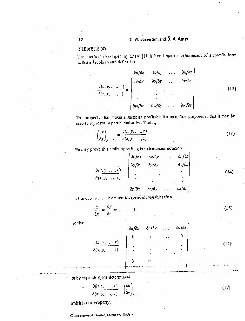
The classical method of eliminating non-measurable thermodynamic properties is successive use of the Maxwell relations. However, this method is very time consuming at times since one does not know exactly in which di-rection the elimination must take place. Sometimes, due to this uncertainty, it does not work There is a method, however, called the method of Jacobians which accomplish the same result in a very systematic way without any guess work, Somerton and Arnas (1985). Although the method was first introduced fifty years prior to this, the only text known that discuss these is that of Callen (1960). This methodology has been used extensively to explain certain thermodynamic phenomena, to design experi-ments, and to eliminate the non-measurable thermodynamic properties, Arnas (2000). The measurable thermo-dynamic properties are p, T, V. Also the specific heats at constant pressure and volume, respectively,

pp T

sTc

and v

v T

sTc

, the coefficient of thermal expansion, pT

v

v

1 , and the isothermal com-

pressibility, T

T p

v

v

1 of substances can be measured. Using these parameters and since thermodynamic

properties are mathematically well behaved functions, namely the order of differentiation does not make any

difference, i.e.

X

Z

YY

Z

Xthe elimination of the non-measurable properties becomes simple.

In general, the Maxwell relations are obtained from {dZ=M dX + N dY} as .YX X

N

Y

M

Since U =

U(S,V) then SV V

UdS

S

UdU

. Comparing this equation to the Gibbs’ equation, {dU=T dS – p dV}, it

is seen that TS

U

V

and pV

U

S

. Additionally, using the above property, we can get the equali-

tyVS S

p

V

T

.

Similar equalities can be obtained using the other Gibbs equations that relate other properties, i.e. enthalpy, H = H (S, p) and {dH = T dS + V dp}, the Gibbs function G = G(T,p) and {dG = - S dT + V dp}, and the Helmholtz potential F = F(T,V) and {dF = -S dT – p dV}. These are also useful in elimination of some of the non-measurable terms and thermodynamic properties.

In Somerton and Arnas (1985), the theory as well as the use of the method is given. For the general equation of {dZ = M dY + N dX}, the Jacobian formulation can be written as {[Z,ξ] = M[Y,ξ] + N[X,ξ]} where ξ is any

other thermodynamic property. Also, the equalities [Z,Z] 0 , [Z,ξ]=-[ξ,Z], and

),(

),(

YX

YX=1 are very useful.

From fundamentals of mathematics we have

X

Y

X

Y

. Using the first law of thermodynamics for a

cycle, we get WQ since 0 dU . In Gibbs form, {dU=TdS – pdV} giving for a cycle [T ds = p

dV] which in Jacobian form becomes [T,S] = [p,V]. The systematic use of these will permit one to convert nonmeasurable terms into measurable ones including p, V, T, cp, cv, α, and κT.

The general methodology, therefore, is:

1. Write down the given in terms of Jacobians. 2. Reduce by Maxwell equations using the various Gibbs equations. 3. Use the definition of cp, cv, α, and κT to further reduce the given equation. 4. If everything is done correctly, the result should only contain p, v, T, cp, cv, α, and κT. If not, an er-

ror has been made; you need to go back and redo everything.

If this methodology is not used, then one goes around and around until a solution is obtained and one does not know if the route taken is the correct one. The advantage of the method of Jacobians is that the result shows if a mistake has been made.

The examples given in Somerton and Arnas (1985) are for learning the methodology. We will also look at other relations and get the physical significance of some other important thermodynamic phenomena, for example

throttling,

VT

VT

cp

T

pph

1 and the speed of sound in any medium,

Tv

p

S

Sv

pv

c

c

v

ppc 22

1.

As an example, start withv

v T

sTc

. Therefore, following the methodology given,

STEP 1.

),(

),(/

),(

),(

),(

),(

),(

),(

Tp

Tv

Tp

vs

Tp

Tp

vT

vs

T

s

v

STEP 2: However, the denominator is by definition {-v κT}. Therefore,

TppTTv

pT

pT

TTv

p

v

T

s

T

v

p

s

vT

s

T

v

p

v

T

s

p

s

vTp

vs

vT

s

1

1

),(

),(1

Using the Maxwell relation, pT

T

v

p

s

which comes from the Gibbs form of the Gibbs’ function equa-

tion, and the definitions of cp, α, and κT,

)((

1 22T

p

T

v vT

cv

vT

c

. Rearranging,

Tvp Tvcc

2

)( .

For an ideal gas, this general result reduces toM

cc vp

)( , where is the Universal gas constant and M is

the molecular mass of the ideal gas, a well known relationship. It is also possible to show that for an incom-pressible substance, i.e. liquid water, 0)( vp cc which says that for those we must just use c as the specific

heat without any subscripts. For those substances for which we have tables, enthalpies must be used and not Tch , another common mistake in literature, Çengel and Boles (2008). In analyzing other derivatives of

interest, these methodologies become very useful as well when we go through those quantities, for example

TV

U

and T

p

H

, and their values for an ideal gas. In Arnas (2000), these along with other characteristics

are further studied. The slope of various functions on the Mollier chart, an (h-s) diagram,

i.e.

pT v

TvT

s

h,

ps

h

, vs

h

, and other thermodynamic diagrams, such as the (p-h) for refrig-

erants, i.e.

T

v

p

s v

p

p

c

c

h

p, is also explained to clarify the physics involved; for an ideal gas, this re-

duces to v

k

v

c

c

h

p v

p

s

, where k is the ratio of the specific heats,

v

p

c

ck .

To obtain pressure-temperature relation for an ideal gas under reversible adiabatic conditions, we start with

sT

ps

sT

sp

T

p

s ,

,

,

,. Substituting for the numerator and the denominator from Jacobian properties, then

we get p

p

p

s v

T

T

c

vp

pTT

c

T

p

],[

],[ which is a general result. Using the ideal gas equation, the partial de-

rivative on the right can be evaluated. Using the difference between the two specific heats for an ideal gas, as

was shown above, the result becomes

1k

k

T

p

MT

pc

T

p p

s

. Therefore, 1/

/

k

k

TdT

pdp which upon

integration gives the well known result

k

k

pT1

. This result is only valid if we have an ideal gas which un-

dergoes a reversible and adiabatic, constant entropy, process. Again, this fact is not trivial and must be kept in

mind before this result can be used. Similar results can be obtained for v

v

s p

T

T

c

T

v

, in general, and

applied to an ideal gas would give,

1

1

/

/

kTdT

vdvor kvT 1 . For

sv

p

we get the result, in gen-

eral, .Ts v

pk

v

p

This equals for an ideal gas kvdv

pdp

/

/ giving kvp .

The total intent in all this was to verify the physics of the situation using mathematics. Mathematics is just a tool to totally explain these physical phenomena that characterize nature. Nature is what physics is; mathemat-ics is the explanation mechanism and nothing more. Design of Experiments

In engineering, experimental verification of analysis or computational results is extremely important. For that, it is necessary to design experiments. Experiments can only be designed for those parameters for which we can make measurements. As was discussed before, the measurable parameters in thermodynamics are p, T, V, cp, cv, α, and κT. Therefore, the designed experiment can only involve these parameters.

As an example of this important issue, consider the Clausius’ equation which is

12

12

vvT

Q

dT

dp

saturation

.

By considering the T-s diagram, it is obvious that the heat transferred is equal to 1212 ssTQ . From the

Gibbs’ equation for enthalpy, {dh = T ds + v dp}, and since at saturation the pressure and temperature are con-

stants, then {dh = T ds} giving .)()( 1212 ssThh Upon substitution,

12

12

vvT

hh

dT

dp

saturation

, where 2

refers to the saturated vapor state, g, and 1 to the saturated liquid state, f. Therefore, the Clausius equation be-

comes, .fg

fg

saturation Tv

h

dT

dp

Clapeyron modified this equation by making certain assumptions. The first assumption is that fg vv which

is an acceptable one since the vapor specific volume is much greater numerically than the liquid specific vol-ume, as can be seen in the Steam Tables, Çengel and Boles (2008). The second assumption is that of an ideal

gas for the vapor, i.e.

p

T

Mvvg which, upon substitution, makes the Clausius’ equation

2T

p

M

h

dT

dp fg

saturation

. Collecting like terms, this equation reduces to

M

h

T

dT

p

dp

fg

2

. Considering

that fgh is a constant, an assumption that needs to be verified for the design of the experiment, and integrating

and simplifying, the Clausius-Clapeyron equation is obtained as

M

h

Td

pd fg

1

ln which is only valid if

fg vv and we have an ideal gas for constant fgh . All of these three assumptions must be satisfied before the

results of the experiment can have any significance. Therefore in the design of the experiment we must consider these facts very carefully.

In designing an experiment, the first assumption for the Clausius-Clapeyron equation is satisfied when one looks in the Steam Tables, Çengel and Boles (2008), to compare the numerical values of the specific volume as a va-por and a liquid. The second assumption, an ideal gas, requires some more discussion. When we look at the compressibility diagram for substances, we see that the compressibility for all substances approach unity, mean-ing they approach the characteristics of an ideal gas, as the reduced pressure of the substance approaches zero,

i.e 1Z as .0Reduced criticalp

pp This result signifies that the experiment must take place at low real pres-

sures, i.e. below atmospheric, since the critical pressure for steam is 22.09[MPa] to make sure that we are ap-proaching zero for the reduced pressure to guarantee ideal gas situation. Finally, constant fgh assumption re-

quires that the measurements must take place at a pressure an increment above and an increment below the saturation pressure under investigation. By taking this increment small and splitting it up for as many precise

measurements as possible, all that is needed to do is to plot (ln p) versus

T

1 using the absolute temperature.

The slope of the line is negative, as the Clausius-Clapeyron equation requires, and will give the value fgh once

the molecular mass of water is used. Other fluids can also be used in this experiment; the only requirement is to

make sure that 1Z and 0Reduced criticalp

pp for the liquid that is used.

For the speed of sound or the Joule-Thomson coefficient similar experiments can be designed, constructed, and experimental results can be obtained once their measurable forms are derived, as was done above. This meth-odology is good for any quantity for which an experiment is to be designed; the important thing to keep in mind

is the assumptions under which the result is obtained. If any one of the assumptions is not met, then the experi-ment will not give the expected results.

This, of course, is not different from any scientific/engineering analysis or experiment. The results obtained are only as good as the assumptions made and that the results are only valid under those assumptions. This may sound trivial but we will show that it is a mistake made quiet commonly by researchers and/or authors of text-books. Errors made in literature

When one studies the literature carefully, one does find fundamental errors made due to the fact that simple un-derstanding of thermodynamics is lacking. As we have already discussed very early on the state principle and the fact that any two independent intensive thermodynamic properties are sufficient to define a thermodynamic state, it is really of no consequence which two are selected since the final result has to be unique. Chawla (1978) selects three different combinations of properties to determine the speed of sound. In the first case, the variables selected are the velocity, the pressure, and the enthalpy. The result for the speed of sound turns out to be

phhp

c

1

12

where ρ is the density, inverse of v. The second case is for the velocity, the density, and the pressure. This time the result obtained becomes

1

2

p

h

h

c p .

The third case is for the velocity, the pressure and the temperature. The result obtained is,

TTp

p

pp

h

c

T

c

1

12 .

However, from the definition of the speed of sound, s

pc

2 and using the methodology given above, it is

indeed very simple to show that the analytical result is Tv

p

s v

p

c

cv

sv

spv

v

pvc

2222

,

,.

No matter which two properties along with the velocity is chosen, this is the result that must be obtained. Re-sults are obtained in terms of nonmeasurable properties which are consequently solved numerically, Chawla (1978). Since the series variation of these properties do not have the same character, numerical truncation errors result in different forms for the answers. The author then tries to justify why they are different. However, we have seen that the result has got to be unique, the state principle, and it is demonstrated once again by Arnas (2000). All three results above analytically are the same, as it should be. Numerically, they are not! Therefore, a fundamental understanding of thermodynamics is very important to explain physical phenomena.

Shortcomings of textbooks

Apart from the shortcomings of books on Thermodynamics, and there are many, similar shortcomings that exist in other textbooks because of lack of being precise that discuss, for example, Heat Transfer which is an applied course heavily dependent on thermodynamic principles. The student is learning from the textbooks; therefore, they trust the contents as they must. However, if the topics are not precisely covered, then they learn the wrong material. As an example, we will consider condensation phenomena since it is an important process in thermodynamics, as we have discussed above in the case of the Clausius-Clapeyron equation and the steam experiment, and since we must design condensers for technological purposes, using heat transfer. When one considers the condensa-tion phenomenon as discussed in textbooks, also as was done by Arnas et. al (2004), there are many assumptions that are made to be able to analyze the physical situation. Unfortunately in all of these, the assumptions that are made are not justified for the final result. The final result is the same in all of the references, the only thing dif-ferent are the symbols used. However, the student does not know if a given situation actually satisfies all the as-sumptions made. Therefore, for all situations, the only design equation is the one found in the texts and that one is used blindly. It is indeed possible to find situations where anyone of these conditions is not met which would make the equation useless. In Arnas et.al (2004) not only is the result obtained very rigorously and in a very clear and analytical fashion, the conditions under which the result is valid are also very clearly given so that the user, the student, researcher or the design engineer is able to ascertain if the problem actually fits the final de-sign equation for convection in condensation.

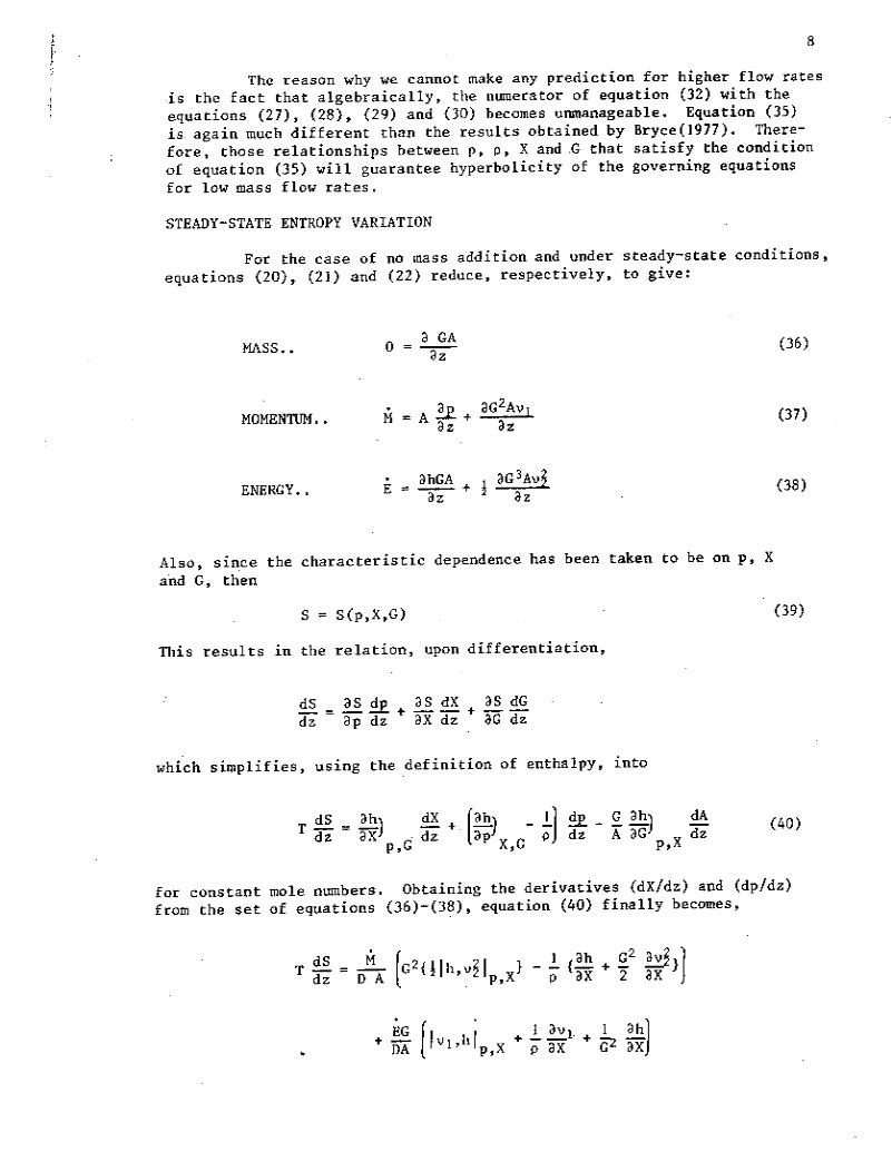
In another study by Arnas et. al (1980), it was shown that the two-phase flow design equations are not usable under all conditions since they tend to decrease the entropy generation for certain combinations of flow rates and geometries; a condition that violates the second law of thermodynamics. Naturally, under those conditions the equations cannot be used for design purposes and other correlations must be searched.

What has been attempted here is to show the importance of correct use of precise thermodynamics in teaching of thermodynamics as well as in all other fields of science and technology. If it is not used precisely, errors are made that could affect the designed equipment or lead to disastrous situations in extreme cases. In engineering we cannot make mistakes since, unlike the doctor, we do not kill one person at a time! Our failures are watched and seen by the whole world, for example the Space Shuttle disaster. We must teach well, in a correct way, and precisely and demand of our students at all levels the same precision in their work, Arnas (2005). Only in that fashion can be sure that the next generation of engineers/scientists understands the critical ramifications of what is at stake. This is more important than anything else that we can teach our students; their understanding and appreciation of the importance of their precise work.

Conclusions In this paper, the precise teaching of thermodynamics has been emphasized since these topics are used in other fields of science and technology. The textbooks must be correct giving the precise description of systems, equa-tions and conclusions. Otherwise the students learn the wrong information and apply it in the same fashion. It has also been shown that methodologies exist for physical interpretation of mathematical expressions in thermo-dynamics by eliminating nonmeasurable quantities such as entropy, designing thermodynamic experiments and investigating various applications in other fields of science and technology that use thermodynamic principles. The emphasis has been in correct and precise work, a quality that we must impose on our students. This type of instruction would ultimately affect students who are aware of the nature, the effect of everyday usage of energy on the environment, and what needs to be done within the restrictions of nature to be sustainable at least at the levels that we enjoy today. Of course, these must be done in all aspects of education not only in the education of engineers, in general, and thermodynamics education, in particular. Success in this will make life better now and forever. The previous pages have emphasized undergraduate work. It is indeed very important to extend this into statis-tical and nonequilibrium thermodynamics for graduate students. The challenges of energy use, pollution and sustainability all depend on clear, precise and correct study of these and appropriate applications. It can and should be pursued very aggressively throughout.

Acknowledgement

The view expressed herein are those of the author and do not purport to reflect the position of the Unites States Military Academy, the Department of the Army, or the Department of Defense.

Nomenclature

A Area [m2]

B Any extensive thermodynamic property

b Any intensive thermodynamic property, b=B/m

c Specific heat [kJ/(kg-K)]; also speed of sound [m/s]

E Energy [kJ]

e specific energy [kJ/kg]

F Helmholtz potential [kJ]

G Gibbs free energy [kJ]

H Enthalpy [kJ]

h Specific enthalpy [kJ/kg]

k Ratio of specific heats, k=(cp/cv)

M Molecular mass [kmol]; also arbitrary function

m Mass [kg]

.

m Mass flow rate [kg/s]

N Arbitrary function

n Unit vector

p Pressure [kPa]

Q Heat [kJ]

Universal gas constant [kJ/(kmol-K)]

S Entropy [kJ/K]

s Specific entropy [kJ/(kg-K)]

T Temperature [K]

t Time [s]

U Internal energy [kJ]

u Specific internal energy [kJ/kg[

V Volume [m3]

v Specific volume [m3/kg]

V Velocity [m/s]

W Work [kJ]

X Arbitrary function

Y Arbitrary function

Z Arbitrary function; also compressibility factor [-]

z Elevation [m]

Greek symbols

α Coefficient of thermal expansion [1/K]

β Coefficient of performance for a refrigerator

γ Coefficient of performance for a heat pump

Δ Difference

δ Increment

η Efficiency for an engine

Θ Angle [o]

κT Isothermal compressibility [1/kPa]

μ Joule-Thomson coefficient [ K/kPa]

ξ Arbitrary thermodynamics property

ρ Density [kg/m3]

σ Entropy generation [kJ/K]

Subscripts

E Engine

CE Carnot engine

CV Control volume

f Liquid phase

fg Phase change from liquid to vapor

g Vapor phase

H High

L Low

v Volume

p Pressure

o Atmospheric

References

[1] Arnas AÖ (2000) On the Physical Interpretation of the Mathematics of Thermodynamics. International Journal of Thermal Sciences 39: 551-555 [2] Arnas AÖ (2005) Education, Energy, Exergy, Environment – Teaching Teachers to Teach Thermodynamics, Proceed-ings, Second International Exergy, Energy and Environment Sysmposium-IEEES2, Kos, Greece, #167. [3] Arnas AÖ, Hendrikson HAM, van Koppen CWJ (1980) Thermodynamic Explanation of Some Numerical Difficulties in Multiphase Flow Analyses, Proceedings, European Two-Phase Flow Group Meeting, Glasgow, Scotland, F4. [4] Arnas AÖ, Boettner DD, Bailey MB (2003) On the Sign Convention in Thermodynamics-An Asset or an Evil, Proceed-ings, ASME-IMECE2003, IMECE2003-41048. Also, Boettner DD, Bailey MB, Arnas AÖ (2006) On the Consistent Use of Sign Convention in Thermodynamics, International Journal of Mechanical Engineering Education 34/4: 330-348 [5] Arnas AÖ, Boettner DD, Benson MJ, van Poppel BP (2004) On the Teaching of Condensation Heat Transfer, Proceed-ings, ASME-IMECE2004, IMECE2004-50277. Also, Tamm G, Boettner DD, van Poppel BP, Benson MJ, Arnas AÖ (2009) On the Similarity Solution for Condensation Heat Transfer, ASME Journal of Heat Transfer 131: 111501-1/5 [6] Callen HB (1960) Thermodynamics, Wiley. [7] Çengel YA, Boles ME (2008) Thermodynamics-An Engineering Approach, 6th Edition, McGraw-Hill. [8] Chawla TC (1978) On Equivalency of the Various Expressions for Speed of Wave Propagation for Compressible Liquid Flows with Heat Transfer, International Journal of Heat and Mass Transfer 21: 1431-1435. [9] Mooney DA (1953) Mechanical Engineering Thermodynamics, Prentice-Hall. [10] Obert EF (1960) Concepts of Thermodynamics, Wiley. [11] Somerton CW, Arnas AÖ (1985) On the Use of Jacobians to Reduce Thermodynamic Derivatives, International Jour-nal of Mechanical Engineering Education 13-1: 9-18. [12] Zemansky MW (1943) Heat and Thermodynamics, Wiley.

Int. J. Therm. Sci. (2000) 39, 551–555 2000 Éditions scientifiques et médicales Elsevier SAS. All rights reservedS1290-0729(00)00249-0/FLA

On the physical interpretation of the mathematicsof thermodynamics 1

A. Özer Arnas *Mechanical Engineering Department, Bogaziçi University, Bebek 80815 Istanbul, Turkey

(Received 26 October 1999, accepted 3 November 1999)

Abstract —The use of mathematical relations is discussed with the idea of enhancing the teaching–learning process inthermodynamics. It is emphasized that the physical interpretation of mathematical relations is of importance in explainingthermodynamic phenomena, showing how thermodynamic tables are made, the physical interpretation of thermodynamic diagrams,the design of experiments, and research in fields that require thermodynamics, particularly for quantities that involve nonmeasurablethermodynamic properties. It is believed that the appropriate use of these relationships contributes to the clear understanding ofthermodynamic concepts, processes and systems. 2000 Éditions scientifiques et médicales Elsevier SAS

thermodynamics / relations / phenomena / tables / diagrams / experiments / research

Nomenclature

c speed of sound . . . . . . . . . . . . . . m·s−1

cp specific heat at constant pressure . . . . kJ·kg−1·K−1

cv specific heat at constant volume . . . . . kJ·kg−1·K−1

h specific enthalpy . . . . . . . . . . . . . kJ·kg−1

k ratio of specific heats,cp/cvp pressure . . . . . . . . . . . . . . . . . . kPa

s specific entropy . . . . . . . . . . . . . . kJ·kg−1·K−1

T temperature . . . . . . . . . . . . . . . . K

V flow velocity . . . . . . . . . . . . . . . m·s−1

v specific volume . . . . . . . . . . . . . . m3·kg−1

X any other thermodynamic property

Greek symbols

ρ density . . . . . . . . . . . . . . . . . . kg·m−3

* Current address: Department of Civil and Mechanical Engineering,United States Military Academy, West Point, NY 10996, USA.io7597@trotter.usma.edu

1 This article is a follow up to a communication presented by theauthor at the ECOS ’98 Seminar held in Nancy (France) in July 1998.

1. INTRODUCTION

In almost all books ofThermodynamics, there is achapter on the “Thermodynamic relations for simplecompressible substances” [1], “Thermodynamic propertyrelations” [2], or “Thermodynamics of a simple com-pressible substance” [3]. This is included, it seems, asan afterthought without following through the physicalinterpretation of the results. The reasons why certainprocesses result in given relations, or why the slopes oflines have the form that they do on certain thermody-namic diagrams can easily be explained by simple phys-ical interpretation of the mathematical analysis of ther-modynamics. Often, the Maxwell equations are obtainedas a consequence of mathematical reasoning rather thanthe physical value of such relations. It is never discussed,however, how thermodynamic experiments can be de-signed, how thermodynamic assumptions must be satis-fied, and how the results may be used.

Research in thermal hydraulics requires the analysesto include various thermodynamic properties and rela-tions [6]. If these are of the nonmeasurable type, then thenumerical integration of these relations lead to differentresults due to the accumulation of errors. Nevertheless,fundamental thermodynamics teaches us that the choiceof these parameters are arbitrary as long as they are inde-

551

A.Ö. Arnas

pendent [1–3]. It is indeed easy, but interesting, to showthat the end result is the same, as it should be, and a sim-ple analysis does prove it very elegantly [7]. In one ofthe examples given below, this is proven. As a matter offact, similar concepts were used to clarify the numericaldifficulties of two-phase flow situations that commonlyarise in nuclear thermal hydraulics as well as two-phasecorrelations that are used for design [8].

There are different ways to solve for or discuss theseuseful relations. Here the method of Jacobians [4] is used.This is a personal preference and other methods may beused equally successfully depending on one’s choice. Themethod is not discussed here; rather it is used to show theresults of some thermodynamic situations of interest.

1.1. Example 1

In this example, the slope of a constant volume linein the superheated region of the Mollier diagram will beinvestigated. The result will be applied to an ideal gas,since steam at elevated temperatures acts as one, and itsfunctional form, in general, will be determined.

The quantity that is to be investigated is(∂h/∂s)vsince theh–s diagram is the Mollier diagram. As a firststep, this relation is written in terms of Jacobians as(

∂h

∂s

)v

= [h,v][s, v] (1)

Then, the terms that involveu, h, g andf , specific in-ternal energy, enthalpy, the Gibbs and Helmholtz poten-tials, respectively, are eliminated by using equations ofthe form

dh= T ds + v dp (2)

written in the form of Jacobians as

[h,X] = T [s,X] + v[p,X] (3)

whereX is any other thermodynamic property. Thus inthis case,

[h,v] = T [s, v] + v[p,v] (4)

Since in a cycle, from the first law,

[T , s] = [p,v] (5)

and since the definition of the specific heat at constantvolume is

cv

T= [s, v][T ,v] (6)

then the combination of equations (1), (4), (5) and (6)gives (

∂h

∂s

)v

= T{

1+ v

cv

(∂p

∂T

)v

}(7)

This result shows that the constant volume line onthe Mollier diagram is that of temperature along with acorrection term. For an ideal gas,(

∂p

∂T

)v

= cp − cvv

(8)

which upon substitution into (7) gives(∂h

∂s

)v

= kT (9)

This, therefore, shows that the slope of the constantvolume line of an ideal gas on the Mollier diagramfollows that of the temperature increased by the factorof the ratio of specific heats. For a given situation, thevalidity of the ideal gas assumption must be investigatedbefore equation (9) can be used. Equation (7), however,is the generalized result and is applicable to steam at anystate.

Other slopes on the Mollier diagram can also beinvestigated to better explain and clarify the physicalinterpretation of the diagram. Similarly, other diagramscan be investigated. The undergraduate and graduatestudents find this approach very useful and learn on theirown the mathematics of the Jacobians in its mathematicalcontext since the physical significance can be betterunderstood.

1.2. Example 2

The relation between the pressure,p, and temperature,T , in a reversible adiabatic process is useful in solvingmany important and interesting problems. The applica-tion of the result to a special case of an ideal gas withconstant specific heats is also very useful in solving manyproblems of significance. Therefore, the relation that isto be investigated can be written as(∂p/∂T )s which be-comes in terms of Jacobians(

∂p

∂T

)s

= [p, s][T , s] (10)

With the use of equation (5) and the definition of specificheat at constant pressure,

cp

T= [s,p][T ,p] (11)

552

On the physical interpretation of the mathematics of thermodynamics

equation (10) reduces to(∂p

∂T

)s

= cpT

(∂T

∂v

)p

(12)

For the case of an ideal gas,(∂T

∂v

)p

= p

cp − cv (13)

Upon substitution into equation (12),(∂p

∂T

)s

= pT

k

k − 1(14)

For the case of an isentropic process, which is the case ofinterest, then

dp/p

dT/T= k

k − 1(15)

results in a relation given as

T = p(k−1)/k (16)

which is valid for an isentropic process of an ideal gaswith constant specific heats. Equation (16) is not onlywell known but also used extensively. Similar resultsbetweenp and v, and T and v can also be obtainedfollowing through a similar procedure.

1.3. Example 3

Maxwell relations can be found from the Jacobiansthemselves and need not be introduced separately. In-deed, the relations are only yet another way of expressingthe integrability condition of a property. Thus for a cyclicprocess in a simple system, the area in ap–v diagram,representing reversible net work out, will transform to thesame area in aT –s diagram, representing reversible netheat in, as in equation (5). In mathematical representa-tion,

∂(p, v)

∂(T , s)= 1 (17)

For example, (∂s

∂p

)T

={∂(s, T )

∂(p,T )

}which when multiplied by equation (17) becomes

(∂s

∂p

)T

={∂(s, T )

∂(p,T )

}{∂(p, v)

∂(T , s)

}={∂(s, T )

∂(T , s)

}{∂(p, v)

∂(p,T )

}reducing to the well known Maxwell relation(

∂s

∂p

)T

=−(∂v

∂T

)p

(18)

It seems to be desirable to introduce Maxwell rela-tions this way since it refers to the fundamental law bywhich energy and its Legendre transformations are in-deed properties or potential functions subject to Maxwellrelations [5].

1.4. Example 4

As an example of design of experiments, consider themeasurement of the speed of sound, which is defined as

c2=(∂p

∂ρ

)s

(19)

whereρ is the density of the medium and is equal tothe inverse of the specific volume. In view of the factthat the entropy is a nonmeasurable quantity, it must beeliminated in favor of those that are measurable. Usingequations (6) and (11), the speed of sound becomes

c2=−k(∂p

∂ρ

)T

(20)

which now is totally measurable. Therefore, an isother-mal experiment must be designed in which the variationin pressure with respect to density must be measured.

Although it is a well known fact that the choice of ther-modynamic properties that characterize a physical situa-tion is arbitrary as long as those properties are indepen-dent, one finds in the literature situations where this factis overlooked in some thermal hydraulics research [6–8].

Assuming that the variables areV, p, andh, whereVis the flow velocity, the speed of sound reduces to [6]

c2= 1

(∂ρ/∂p)h + (1/ρ)(∂ρ/∂h)p (21)

The first term is obtained as(∂ρ

∂p

)h

=−(ρ2)

(∂v

∂p

)h

=−(ρ2)[h,v][h,p] (22)

553

A.Ö. Arnas

With the use of equations (4), (6) and (11), it can beshown that equation (22) reduces to(

∂ρ

∂p

)h

=−(ρ2)

{1

k

(∂v

∂p

)T

− 1

ρcp

(∂v

∂T

)p

}(23)

From equations (4) and (11), it follows that the secondterm of equation (23) can be expressed as

1

ρ

(∂ρ

∂h

)p

=− ρcp

(∂v

∂T

)p

(24)

When equations (21), (23) and (24) are combined, equa-tion (20) is obtained.

Assuming the variables areV, ρ, andp, the speed ofsound reduces to [6]

c2= −ρ(∂h/∂ρ)pρ(∂h/∂p)ρ − 1

(25)

The numerator is the inverse of equation (24). Since(∂T

∂p

)ρ

(∂p

∂ρ

)T

(∂ρ

∂T

)p

=−1 (26)

the denominator of equation (25) can be written as

ρ

(∂h

∂p

)ρ

− 1= ρ [h,ρ][p,ρ] − 1= cvρ(∂T

∂p

)ρ

(27)

where equations (4) and (6) are used. When equations(24), (25) and (27) are combined, equation (20) isobtained.

Assuming the variables asV, p, andT , the speed ofsound reduces to [6]

c2={[−(∂ρ/∂T )p

ρcp

][ρ

(∂h

∂p

)T

− 1

]+(∂ρ

∂p

)T

}−1

(28)

The only term to analyze is[ρ(∂h/∂p)T − 1] whichsimplifies to[

ρ

(∂h

∂p

)T

− 1

]=−(Tρ)

(∂v

∂T

)p

(29)

where equations (4) and (17) are used. From the iden-tity [3]

(cp − cv)= T(∂v

∂T

)p

(∂p

∂T

)v

(30)

and the equations (28) and (29), equation (20) follows.

It is, therefore, obvious that no matter what propertiesare chosen, the final result is unique because of the funda-mental concepts of thermodynamics [7]. However, if theresults in [6] were not reduced in this fashion, they wouldhave to be evaluated numerically. Since the series repre-sentation of enthalpy, entropy and other nonmeasurableterms are not similar, the numerical solutions of equa-tions (21), (25) and (28) will give different results. Thejustification for it was attempted [6]. It is now proven thatthat attempt is really a communication that has absolutelyno thermodynamic basis [7].

It is, therefore, seen that the method of Jacobians isindeed a very powerful one to simplify the various math-ematical relations encountered in the study of thermody-namics and gives them physical significance. It is thisphysical significance that further increases the appreci-ation that the students have for thermodynamic reason-ing and, as a result, they can better relate, understand andlearn thermodynamics [10–12] and makes the teaching ofthe subject more pleasurable.

Other experiments can also be designed using thetechniques and methodologies developed above and inthe literature. In the past, along with the speed of sound,experiments have been designed for the Joule–Thomsoncoefficient and the Clausius–Clapeyron equation withgreat success and enthusiasm.

2. CONCLUDING REMARKS

It is indeed obvious that the applications of these tech-niques are very meaningful and give even further in-sight to why and how things happen. When the student istaught these methodologies, the learning should improve.If the mathematical topics are approached in this fashion,the thermodynamic concepts and equations make moresense [9].

These concepts and methodologies have been usedfor undergraduates, and graduate students, with extremesuccess in the United States, Belgium, the Netherlands,Italy and Turkey. The students have been able to relate tothermodynamics better once they see and understand thereasons behind the natural happenings.

REFERENCES

[1] Moran M.J., Shapiro H.N., Fundamentals of Engi-neering Thermodynamics, 4th Edition, Wiley, 2000.

[2] Çengel Y.A., Boles M.A., Thermodynamics: An Engi-neering Approach, 3rd Edition, WCB/McGraw-Hill, 1998.

554

On the physical interpretation of the mathematics of thermodynamics

[3] Huang F.F., Engineering Thermodynamics: Funda-mentals and Applications, 2nd Edition, Macmillan Publish-ing Company, 1988.

[4] Somerton C.W., Arnas A.Ö., On the use of Jacobiansto reduce Thermodynamic derivatives, Int. J. Mech. Eng.Educ. 13 (1985) 9–18.

[5] Lewins J.D., Jacobians in Thermodynamics, Letterto the Editor, Int. J. Mech. Eng. Educ. 14 (1986) 74–75.

[6] Chawla T.C., On equivalency of the various expres-sions for speed of wave propagation for compressible liq-uid flows with heat transfer, Int. J. Heat Mass Tran. 21(1978) 1431–1435.

[7] Arnas A.Ö., On the thermodynamic uniqueness ofthe choice of coordinates for compressible liquid flow withheat transfer, in: Actes des 5èmes Journées Européennes

de Thermodynamique Contemporaine, Toulouse, France,1997, pp. 27–32.

[8] Arnas A.Ö., Hendriksen H.A.M., van Koppen C.W.J.,Thermodynamic explanation of some numerical difficultiesin multiphase flow analyses, in: Proceedings of EuropeanTwo-Phase Flow Group Meeting, Glasgow, Scotland, 1980,F4.

[9] Tuttle E.R., A simple method for presenting Ther-modynamic partial derivatives to undergraduates, Int. J.Mech. Eng. Educ. 25 (1997) 137–146.

[10] Callen H.B., Thermodynamics, Wiley, 1960.[11] Bejan A., Advanced Engineering Thermodynamics,

Wiley, 1997.[12] Carrington G., Basic Thermodynamics, Oxford Uni-

versity Press, 1994.

555

lna. J. lieat Mass Tm&r. Vol. 21, pp. 1431-1435 Pergamon Press Ltd. 1978. Printed in Great Britain

ON EQUIVALENCY OF VARIOUS EXPRESSIONS FOR SPEED OF WAVE PROPAGATION FOR

COMPRESSIBLE LIQUID FLOWS WITH HEAT TRANSFER

T. C. CHAWLA

Reactor Analysis and Safety Division, Argonne National Laboratory, Argonne, IL 60439, U.S.A.

(Received 22 March 1978 and in revised form 31 March 1978)

Abstract-It is demonstrated that for a compressible flow model with heat transfer, the introduction of a specific state equation to supplem~t the ~ntin~ty, rnorn~t~ and enthalpy equations, leads to a very specific form of an expression for a speed of wave propagation. Consequently, the numerous expressions obtained for various choices of state equations are not easily identifiable and, therefore, can not be evaluated directly in terms of measurable properties. By utilizing the various thermodynamic relationships, we have shown that these expressions are all equivalent and are identifiable as isentropic sonic velocity. As a corotlary to this demonstration, we have also obtained expressions in terms of measurable properties for various ~e~od~~ic-site variables occurring in the coefficients of the gov~ing equations. These expressions are required ifloss in accuracy owing to noise introduced in the direct numerical differentiation of

the derivatives that these state-variables represent is to be avoided.

NOMENCLATURE

flow cross-sectional area ; speed wave propagation defined by equation (11); = (dh,@T),, specific heat at constant pressure; = (&J/~T),, specific heat at constant volume ; speed of wave propagation defined by equation (15); acceleration due to gravity; specific enthalpy ; pressure ; = qwS,lA ; heat flux ;

heated or wetted perimeter ; specific entropy ; temperature of a liquid coolant ; time ; specific internal energy; fluid velocity ; coordinate in the vertical direction.

Greek symbols

UP’ - (dpJaT),/p, coefficient of thermal expansion ;

B F, (~~/~~)=/~, isothe~al coefhcient of bulk compressibility;

P S9 (ap/8P),/p, adiabatic coefficient of bulk compressibility;

Y”? (@PT),, thermal pressure coefbcient ;

A T ? (a~/ap~= ;

1 P’ f/R,;

I P’ ww), ;

P1 fluid density;

z WI wall shear stress;

@ W? vr,,S,fA ; 4 speed of wave propagation as

defined by equation (22).

INTRODUCTION

THE COMPRESS~E liquid flow with heat transfer occurs in numerous nuclear reactor applications. For example, loss of flow resulting from pipe rupture both in the case of boiling water and pressurized water reactors, and also in the ease of liquid metal cooled fast breeder reactors (LMFBRs) requires the modeling of compressible liquid flow with heat transfer. The dy- namics of the coolant, subsequently to the release of molten fuel in the coolant channels during a power transient in an LMFBR, are generally analyzed in terms of compressible coolant flow with heat transfer. The governing equations are solved either by the use of finite-difference methods or by the method of charac- teristics. In both schemes, one needs to determine the speed of wave propagation as a function of tabulated properties of the liquids. In the explicit form of flnite- difference methods (such as Lax method, two step Lo-W~droff difference method, donor-cell type dif- ferent method), one needs speed of wave propagation to determine the size of time steps that satisfies stability criterion [I]. In the case of method of characteristics, the speed of wave propagation is required to determine the slopes of the characteristics. In this latter appli- cation, the form of the expression for the speed of wave propagation varies with the exact form of governing equations chosen for solution. Very frequently, these expressions have very diverse form and do not permit direct numerical evaluation in terms of the properties tabulated in the standard tables. In addition, the algebraic manipulation involved to obtain the govem-

1431

1432 T.C. CHAWLA

ing equations in a form suitable for application of a given numerical method (such as the method of ch~a~te~stics) leads to very compIex forms of coef- ficients of the various terms of the resultant gove~ing equations. These coefficients, generally, are both func- tion of flow parameters and of the physical properties of the coolant. The purpose of the present note is to demonstrate various expressions arrived at in most common formulations of the governing equations for compressible liquid flow with heat transfer are equiva- lent and are identifiable with very famifiar expression, namely a 2 = @P/L@), = I/p& (see Nomenclature for definition of symbols) for the speed of sound defined for the isentropic process of state change and fluid Row. As a corollary to this demonstration, we will show how the various ~oe~~ents which depend only on the properties, can be expressed in a form suitable for direct numerical evaluation by the use of tabulated or measured properties.

FORMULATION

The most common form of the basic governing equations, which are utilized to describe flow through a coolant channel of constant cross-sectional area during a transient such as initiated by loss of flow due to pipe rupture, is [2-41:

P = P(h, PI3 (da)

or

P = p(T, P), (4b)

h = Mp, P), (k)

or

h = h(T, P). (4d)

If we utilize the first equation of state (4a), we can make equations (l)-(3) explicit in variables v, P, h. The use of third state equation (4c) will render equations (l)-(3) explicit in p, u and P. Depending upon the choice of a specific form of state equation as we will illustrate below, we arrive at different expressions for the speed of wave propagation.

Explicit in UAr~Ab~~ v, P, h The use of first state equation (4a) in equation (I)

gives

where

(6)

The use of equation (1) into equations (2) and (3) yields,

where

Combining equations (5) and (8) first to eliminate h between them and second to diminate P between them :

(9)

ah dh 2 dv R,a2 z+v(;z-+a ~~=~-tQ,+@,), (10)

where

1

a = jR,fR,/p)‘:2.

We will show, subsequently, that the above ex- pression defines the isentropic sonic velocity cor- responding to the system of equations (7), (9) and (10) which are explicit in U, P and h. We may note, here, that properties R, and R, as defined by equation (6) are not directly measurable properties. It is clear that the numerical evaluation of these properties is required not only for the determination of quantity a but also for determining coefficients in the governing equations (9) and (30).

Explicit in ua~~ables p, v, P. From the state equation (4c), we have

dh = I,dp+E.,dP.

The use of equation (12) into equation (8) yields

Wf

= Q,+Q,. (13)

Eliminating the terms involving p in equation (13) by using equation (l), we obtain

where

The above expression also defines isentropic sonic velocity, although the form of the expression is not a very familiar one. In the subsequent analysis, we demonstrate that the above is indeed isentropic sonic velocity. Once again, properties i, and A, are not directly measurable quantities, therefore, unless we can demonstrate that expression (15) indeed repre-

Equivalency of wave propagation with heat transfer

sents an isentropic sonic velocity, we will not be able to calculate satisfactorily the numerical values for the quantity c. Thus, if one wants to utilize the system of equations (1 ), (7) and (14) which are explicit in p, u and P, one must numerically evaluate the quantity c as defined by expression (15).

1433

equation (6) and from the definitions of ap and C,, we can write

Explicit in variables v, P, T From state equation (4b), we can write

dp = -pa,dT+p&-dP. (16)

The use of equation (16) into equation (1) yields

(17)

From state equation (4d), we have

dh = C,dT+A,dP. (18)

The use of equation (18) into equation (8) gives

The t julbination of equations (17) and (19) gives

a0 a a2 g+“;+pLyP C (Q,+%), (20)

P a7 az- P&---l *25B,n2 -(Q,+W, (21) at YG- c, aZ c,

where

1 R=

(

p&-l . (22)

m%+~s 1’2 P >

Equations (20), (21) together with equation (7) repre- sents a system of equations that are explicit in P, Tand u. This system has necessitated the introduction of parameter R as defined by equation (22). Although not recognizable as it is defined in the form (22), but it will be shown subsequently that R is the isentropic sonic velocity. We, also, further recognize in view of the third term of equation (21) the need for numerical evalu- ation of quantity Ar.

EVALUATION OF VARIOUS PARAMETERS IN TERMS OF

MEASURABLE PROPERTIES

Various thermodynamic-state variables such as a, c, Q, R,, A,, A,, AT, and R, as introduced previously must be expressed in terms of measurable or derived proper- ties for their evaluation.

Parameters R, and 1,

The relationships (30) and (31) will enable us to evaluate L, and R,, respectively, in terms of either directly measurable properties or properties that can

From the definition of the narameter R. as aiven bv ,. - I be derived from other measured properties (see for

RI=(g)ig)r= -7. (234

From equation (23a), we obtain

1, = -c,. pa,

Equation (23) will permit us to determine Rk and 1, since p, C, and ap are either tabulated in properties tables (see for example Padilla [SJ) or can be derived from other measurable properties [S, 63.

Parameters R, and 1, From equations (4a) and (12), we can obtain

R= !!. P 0 ap h

The use of thermodynamic relationship

h = u+P/p

yields

ah 0 - ap p = 5,‘.

Y, P

(24)

(25)

(26)

From the state equations (4), one can readily derive.

(27)

Substituting for yv from equation (27) and for C, = Cp&//?T (see [6] for the derivation of this re- lationship) into equation (26) we have

ah 0 - ap p

=c &+L Pa, p’ (28)

The use of the following relationship whose derivation can be found in [6] and [7]

BT-B,=z (29) P

into equation (28) yields finally

(30)

Substituting equations (23), (30) and (29) into equation (24) gives

R, = p/9,+$. P

(31)

1434 T. C. CHAWLA

example [S]). For example, /I, is directly measurable or can be determined from the measurements of sonic velocity [5,6].

Theuseofequation (3l)and (23a~into~uation (II) gives

1 1 i?P 10 a=

( > It,+: l/2 =(pps)lla= dp s ! ) . (321

fore, can be evaluated in terms of measurable proper- ties. We have also derived expressions for various thermodynamic-state variables occurring in the coef- Ercients of the governing equation, in terms of measur- able and/or derived properties. The need for such expressions can hardly be overemphasize in view of the fact that direct numerical calculations of the derivatives that these state variables represent will introduce noise and, therefore, their accuracy will be suspect. The substitution of equations (23b), (30) and (29) into

equation (IS) yields

1 -pl, If2 ( ) dP ?-I2 C=

P&J-l =0”‘2= dp $ ( > ’ (33)

Clearly, expressions (1 f ) and (15) have become iden- tifiable namely, each of them defines isentropic sonic velocity.

~~kn~~,led~~rne~ts-~y special thanks are to Mamoru lshi: for his comments on the manuscript. Some useful discussions with Adrian Tentner are greatly appreciated. The work was performed under the auspices of the U.S. Department of Energy.

Substituting the folIo~ng relation for A, whose derivation can be found in f6], 1. I _

A,= g ( > (34) T = f (1 - TGL*), 2.

and equation (29) into equation (22) gives

1 SP Ii2 8=@8,)“2= ap s ( > (35)

3 _.

The expression (22), for Q, thus, becomes recognizable. 4.

5. CONCLUSIONS

By utilizing various the~odynamic relations, we have been able to demonstrate that the various 6.

expressions for the speed of wave propagation intro- 7. duced due to specific choices of a state equation, are identi~able with isentropic sonic velocity and, there-

G. K Leaf and T. C. Chawfa, A survey of numerical methods for hydraulic transients, ANL-77-81, Argonne National Laboratory (1977). J. E. Meyer, Hydrodynamic models for the treatment of reactor thermal transients, ivucl. Sci. ~ngng 10, 269 (1961). A. M. Tenter, An improved numerical analysis of transient two-phase phenomena using a slip model. Ph.D. Thesis, University of Cincinnati (1977). T. C. Chawla and M. Ishii, Equations of motion for two- phase tlow in a pin bundle of a nuclear reactor, fnc. J. Neat Mass Transfir, to be published. A. Padilla, Jr., High-tem~rature thermodynamic prop- erties of sodium, ANL-8095, Argonne National Lab- oratory (1974). J. S. Rowlinson, Liquids UM~ Liquid Mixtures. 2nd Edn, pp. 1 l-17. Plenum Press, New York (1969). W. C. Reynolds and 11. C. Perkins, ~ngin~~ri~g Thermodynamics, 2nd Edn, pp. 262-269. McGraw-Hill, New York (1977).

SUR L’EQUIVALENCE DE PLUSIEURS EXPRESSIONS DE LA VITESSE DE PROPAGATION DUNE ONDE POUR DES ECOULEM~NTS DE LIQUIDES COMPR~SSI~L

ES AVEC TRANSFERT DE CHALEUR

R&urn&--On montre que pour un modtle d’ecoulement compressible avec transfert de chaleur, l’in~oduct~on dune equation d’etat specifique en supplement des equations de continuite, de quantit de mouvement et d’enthalpie, conduit a une forme trb spQifique d’expression pour la vitesse de propagation dune onde. En consequence, les nombreuses expressions obtenues Pour di%rents choix d’cquations d’etat ne sont pas aisement identifiables et ne peuvent itre CvaIuees directement en fonction des proprittes mesurables. En utihsant les relations de la thermodynamique, iI est montre que ces expressions sont to&es ~u~valentes et identifiably g la vitesse du son isentropique. Comme corrolaire a cette demonstration, des expressions sont obtenues en termes de proprietiis mesurables Pour plusieurs variables the~~ynam~ques d’etat intervenant darts tes coefficients des equations du probltme. Ces expressions sont n&.zessaires si l’on veut iviter la perte de precision introduite dam la diffbrentiation numerique

directe de grandeurs derivees que les variables d’etat representent.

ZUR GLEICHWER~GK~IT VERSCHIEDENER AUSDRUCKE FiiR DIE GESCHWINDIGKEIT DER WELLENAUSBREITUNG BEI KIMPRESSIBLEN

FL~SSIGKEITSSTR~~UNGEN MIT W~RM~~BERGANG

Zwmnfnssung-Es wird gezeigt, daR die Einfiihrung einer spezifischen Zustandsgleichung zur Ergiinzung der Kontinuitiits-, Impuls- und ~nthalpiegleichungen bei dem Model1 einer kompressibien St&mung mit Warmeiibergang zu einer sehr spezifischen Gleichungsform fur die Welenausbreitung- sg~ch~n~gk~t fiihrt. Folglich lassen sich die zahlreichen Ausdriicke, die man bei Verwenduug der unterschiedlichen Zustandsgleichungen erhiift, nicht einfach als gleich erkennen und konnen de&& such

Equivalency of wave propagation with heat transfer

nicht direkt nach megbaren Gr6Ben aufgeliist werden. Durch die Anwendung der verschiedenen thermodynamischen Beziehungen haben wir gezeigt, dag alle diese Ausdriicke gleichwertig sind und als isentrope Schallgeschwindigkeit gedeutet werden konnen. Als Folge dieser Darstellung erhielten wir such Ausdriicke aus megbaren Eigenschaften fur verschiedene thermodynamische Zustandsvariablen, die in den Koeffizienten der maBgebenden Gleichungen auftreten. Diese Ausdriicke werden benotigt, wenn GenauigkeitseinbuBen vermieden werden sollen, die auf das Auftreten von Instabilitlten bei der direkten numerischen Differentiation der Ableitungen, die diese Zustandsvariablen darstallen, zuruckzufiihren

1435

sind.

06 3KBIIBAJIEHTHOM XAPAKTEPE BbIPAJKEHIlfi )JJIJI CKOPOCTII PAUIPOCTPAHEHBJI BOJIHbI B IIOTOKE CTMMAEMOZi WIJIKOCTI?

l-IPkI HAJIWIMM TEIIJIOOBMEHA

iklHOTiWWJ - nOKa3aH0, ‘IT0 npEi OnJiCaHJiH TeYeHHR CXGiMaeMOi XGJnKOCTJi C TenJI006MeHOM

flO6aBJJeHHe KOHJCpeTHOrO ypaBHeHJiR COCTOflHEiR K ypaBHeHHRM COXpaHeHBR MaCCbI, JiMJTy~bCa H

3JieprJiEJ np&JBOZViT K OYeHb CneLWjJJiYeCKOfi CfJOpM.2 BblpUeHHJJ &‘JJJ CKOpOCTH paCJJpOCTpaHeHHJJ

BOJIHbI. BcJJeilCTBtie 3TOJ.O MHOrOYJiC~eHHbIe Bblpa~eHJfR, nOJIyYeHHbIe npH WCnOJIb30BaHWB pas-

JlWYHbJX ypaBHeHHfi COCTOIIHWJI, OKa3bIBaJOTCR TpynHO Ji~eHTEJ@WipyeMbIMJJ H HenpHrOAHbIMJf BJJJJ

npO~lJeJiJiJI paCYCTOB B TepMJJHaX HenOCpeeFTBeHHO H3MepXeMbIX BeJIWYJiH. kiCnOJJb3yR pa3nJiYJJbIe

TepMOAJiHaMJiYeCKHe COOTHOIIIeHHR, aBTOpb1 JIOKa3anH, ‘JTO BCe 3TU BbIpaXEHAI RBIIIIEOTCR 3KBH-

BaJIeHTHbJMW Ji OnpeneJJSIJOT 83 3HTpOIJkJYEKykO CKOpOCTb 3ByKa. &JR nOnTBepZ%neHHJJ AaHHOrO

BbIBOAa nOJJyYeHb1 BbIpameHBR B TepMHHaX HeI’IOCpeWTBeHHO Ji3MepJJeMbIX BeJIHWiH mJI pa3nHYHbIX

TepMOAEiHaMJiYeCKHX napaMeTpOB, BXOAJJJIJJIX B K03@&iUHeHTbI WCXOAHbJX ypaBHeHHi. 3TIL BbIpa-

W(eHHII Tpe6ytoTCa B TeX CnyYaJJX, KOrna HeO6XOnJiMO H36encaTb nOTepH TOYHOCTH H3-3a B‘,3H”Ka-

JOIJIHX norpeIIJHoCTek npn npRMOM YWCneHHOM LW@~epeHUHpOBaHEIH npOJi3BOpHbIX, npeACTaB,JeHHbIX

yKa3aHHbJMli napaMeTpaMIi COCTOIIHAJJ.