on the origin of diverse aftershock mechanisms …dkilb/papers/kilb_etal_1997.pdfon the origin of...

Geophys. J . Int. (1997) 128,557-570

On the origin of diverse aftershock mechanisms 1989 Loma Prieta earthquake

following the

D. Kilb,' M. Ellis,' J. Gomberg2 and S. Davis3 Center for Earthquake Research and Information, The University ofMemphis, Memphis, TN, USA. E-mail: [email protected] U S Geological Survey, Memphis, T N , USA CIRESINOAAINGDC, University of Colorado, Boulder, CO, U S A

Accepted 1996 October 16. Received 1996 July 23; in original form 1996 February 15

SUMMARY We test the hypothesis that the origin of the diverse suite of aftershock mechanisms following the 1989 M 7.1 Loma Prieta, California, earthquake is related to the post- main-shock static stress field. We use a 3-D boundary-element algorithm to calculate static stresses, combined with a Coulomb failure criterion to calculate conjugate failure planes at aftershock locations. The post-main-shock static stress field is taken as the sum of a pre-existing stress field and changes in stress due to the heterogeneous slip across the Loma Prieta rupture plane. The background stress field is assumed to be either a simple shear parallel to the regional trend of the San Andreas fault or approximately fault-normal compression. A suite of synthetic aftershock mechanisms from the conjugate failure planes is generated and quantitatively compared (allowing for uncertainties in both mechanism parameters and earthquake locations) to well- constrained mechanisms reported in the US Geological Survey Northern California Seismic Network catalogue. We also compare calculated rakes with those observed by resolving the calculated stress tensor onto observed focal mechanism nodal planes, assuming either plane to be a likely rupture plane.

Various permutations of the assumed background stress field, frictional coefficients of aftershock fault planes, methods of comparisons, etc. explain between 52 and 92 per cent of the aftershock mechanisms. We can explain a similar proportion of mechanisms, however, by comparing a randomly reordered catalogue with the various suites of synthetic aftershocks. The inability to duplicate aftershock mechanisms reliably on a one-to-one basis is probably a function of the combined uncertainties in models of main-shock slip distribution, the background stress field, and aftershock locations. In particular, we show theoretically that any specific main-shock slip distribution and a reasonable background stress field are able to generate a highly variable suite of failure planes such that quite different aftershock mechanisms may be expected to occur within a kilometre or less of each other. This scale of variability is less than the probable location error of aftershock earthquakes in the Loma Prieta region.

We successfully duplicate a measure of the variability in the mechanisms of the entire suite of aftershocks. If static stress changes are responsible for the generation of aftershock mechanisms, we are able to place quantitative constraints on the level of stress that must have existed in the upper crust prior to the Loma Prieta rupture. This stress level appears to be too low to generate the average slip across the main- shock rupture plane. Possible reasons for this result range from incorrect initial assumptions of homogeneity in the background stress field, friction and fault geometry to driving stresses that arise from deeper in the crust or upper mantle. Alternatively, aftershock focal mechanisms may be determined by processes other than, or in addition to, static stress changes, such as pore-pressure changes or dynamic stresses.

Key words: aftershocks, Loma Prieta.

0 1997 RAS 557

558 D. Kilb et al.

INTRODUCTION

The cause of the diverse suite of aftershock focal mechanisms of the 1989 M7.1 Loma Prieta earthquake has not been uniquely resolved (Michael, Elsworth & Oppenheimer 1990; Beroza & Zoback 1993; Zoback & Beroza 1993; Savage, Lisowski & Svarc 1994; Kilb, Ellis & Gomberg 1994). Aftershock locations are frequently related to static stress changes associated with the slip distribution on the main rupture (e.g. Oppenheimer, Reasenberg & Simpson 1988; Mendoza & Hartzell 1988; Beroza 1991; Stein, King & Lin 1992; King, Stein & Lin 1994; Lay & Wallace 1995). The origin of aftershock faulting mechanisms, however, is less well understood. Aftershock mechanisms show significant diversity both temporally and spatially (Oppenheimer 1990; Dietz & Ellsworth 1990; Beck & Patton 1991), a characteristic shared by aftershocks of many large earthquakes, e.g. 1992 M7.3 Landers (King et al. 1994), 1987 ML5.9 Whittier (Hauksson & Jones 1989; Michael 1991), 1985 M6.1 Kettleman Hills (Ekstrom et al. 1992), 1984 M 6.2 Morgan Hill (Oppenheimer et al. 1988), 1984 ML5.8 Round Valley (Priestley, Smith & Cockerham 1988), 1983 M,7.3 Borah Peak (Richins et al. 1987) and 1983 ML6.7 Coalinga (Michael 1987).

Beroza & Zoback (1993) have argued that the slip distribution of the Loma Prieta earthquake cannot explain the mixed suite of aftershock mechanisms, and that they are related instead to an approximately fault-normal, uniform, post-main-shock stress field (Beroza & Zoback 1993; Zoback & Beroza 1993). It has also been suggested that aftershock mechanisms of the 1989 Loma Prieta earthquake were related predominantly to the main-shock slip distribution (Oppenheimer 1990; Michael et al. 1990), and those of the 1992 Landers earthquake to the main- shock slip distribution in combination with the background stress field (Stein et al. 1992; King et al. 1994).

Each of these analyses made different assumptions and applied different criteria to demonstrate quantitatively the origin of aftershock mechanisms. Michael et al. (1990) showed the existence of a heterogeneous stress field but did not tie its origin to the main-shock slip distribution. Examination of the Landers aftershocks (Stein et al. 1992; King et al. 1994) was restricted to a planform (essentially 2-D) analysis. In their study of Loma Prieta aftershocks, Beroza & Zoback (1993) and Zoback & Beroza (1993) posed a simpler hypothesis with less stringent test criteria, and their analysis did not explicitly specify a background stress field.

We evaluate the hypothesis that aftershock mechanisms reflect the sum of pre-existing background stress and static stress changes caused by the main-shock slip. In particular, we examine the extent to which heterogeneity of main-rupture slip within a specific background stress field can explain the diverse mechanisms observed in the aftershock sequence of the M 7.1 Loma Prieta earthquake. The important assumptions we make include: (1) aftershocks occur independently of each other; (2) dynamic processes (such as fluid flow, seismic wave propagation, etc.) do not exert a significant control on the diversity of aftershock mechanisms; and (3) the background stress field and friction on all faults are uniform.

THE 1989 LOMA PRIETA, CALIFORNIA, EARTHQUAKE AND ITS AFTERSHOCKS

The M7.1 Loma Prieta earthquake initiated at a depth of - 18 km under the Santa Cruz Mountains (37.04"N, 121.88"W)

on 1989 October 18th at 00:04 UT and ruptured a plane striking at - 130" and dipping steeply 70" towards the south- west (Hanks & Krawinkler 1991, and references therein). A variety of slip distributions based on inversion of strong ground motions and geodetic data have been proposed (Hartzell, Stewart & Mendoza 1991; Wald, Helmberger & Heaton 1991; Steidl, Archuleta & Hartzell 1991; Beroza 1991; Arnadottir & Segall 1994; Horton, Anderson & Mendez 1995). All of these suggest that slip was extremely heterogeneous and was restricted to a depth range of - 4 to - 18 km.

Our data set includes approximately six months of well- constrained aftershock mechanisms, dating from the main shock to June 1990, taken from the US Geological Survey Northern California Seismic Network (NCSN) catalogue. Mechanisms in the NCSN catalogue are derived from P-wave first motions using the FPFIT algorithm of Reasenberg & Oppenheimer ( 1985). We consider only those aftershocks whose fault parameters (strike, dip and rake of slip vector) were determined to within +30" at a 90 per cent confidence level. Vertical and horizontal formal hypocentral errors are of the order of 0.6 and 0.3 km, respectively. We examine aftershocks within a rectangular region enveloping the fault 40 km along and 20 km perpendicular to strike (Fig. 1). Of a possible 4623 events that fell within the region, 552 satisfied the 90 per cent confidence criterion.

NUMERICAL EXPERIMENTS

To investigate the aftershock response to perturbations in the static stress field induced by the Loma Prieta main shock, we first calculate a net stress field that combines the influence of heterogeneous slip and a uniform background stress field. We then compare the net stress field with aftershock mechanisms in two ways. First, we generate a synthetic aftershock mechanism catalogue based on the theoretical orientation of failure planes within the net stress field assuming a Coulomb failure criterion. The Coulomb failure criterion is used only as a means of calculating the geometrical aftershock parameters (strike, dip and rake of slip vector) and not as a test of whether failure will occur. Synthetic mechanisms are quantitatively compared to those in the observed mechanism catalogue. Second, we attempt to explain the observed mechanisms directly by resolving the net stress field on each of the observed nodal planes and by comparing the predicted and observed rakes. In these comparisons, we consider either nodal plane of the observed focal mechanism to be a likely candidate for the rupture plane. Faulting patterns in strike-slip environments are well known to be complex, and there is no reason to prefer a priori either nodal plane (e.g. Tchalenko 1970; Price & Cosgrove 1990; Savage 1994).

We assume a uniform rather than a heterogeneous background stress field and justify this on two counts. First, the strains and stresses in the Loma Prieta region have accumulated uniformly since the 1906 San Francisco earthquake (Lisowski, Savage & Prescott 1991; Bodin & Bilham 1994). Second, it is debatable whether the 1906 earthquake entirely relaxed the elastic strain field in the Loma Prieta region (Marshall, Thatcher & Lisowski 1994) or left a strain deficit (Bodin & Bilham 1994). Given this uncertainty, we reasonably begin with the simplest set of plausible assumptions, namely, a uniform background stress field.

Each numerical experiment requires the specification of (1) a uniform background stress field representing the regional

0 1997 RAS, GJI 128, 557-570

Loma Prieta's diverse aftershock mechanisms 559

37" 30'

37" 00'

36" 30 122" 3 0 122' 00 121" 3 0

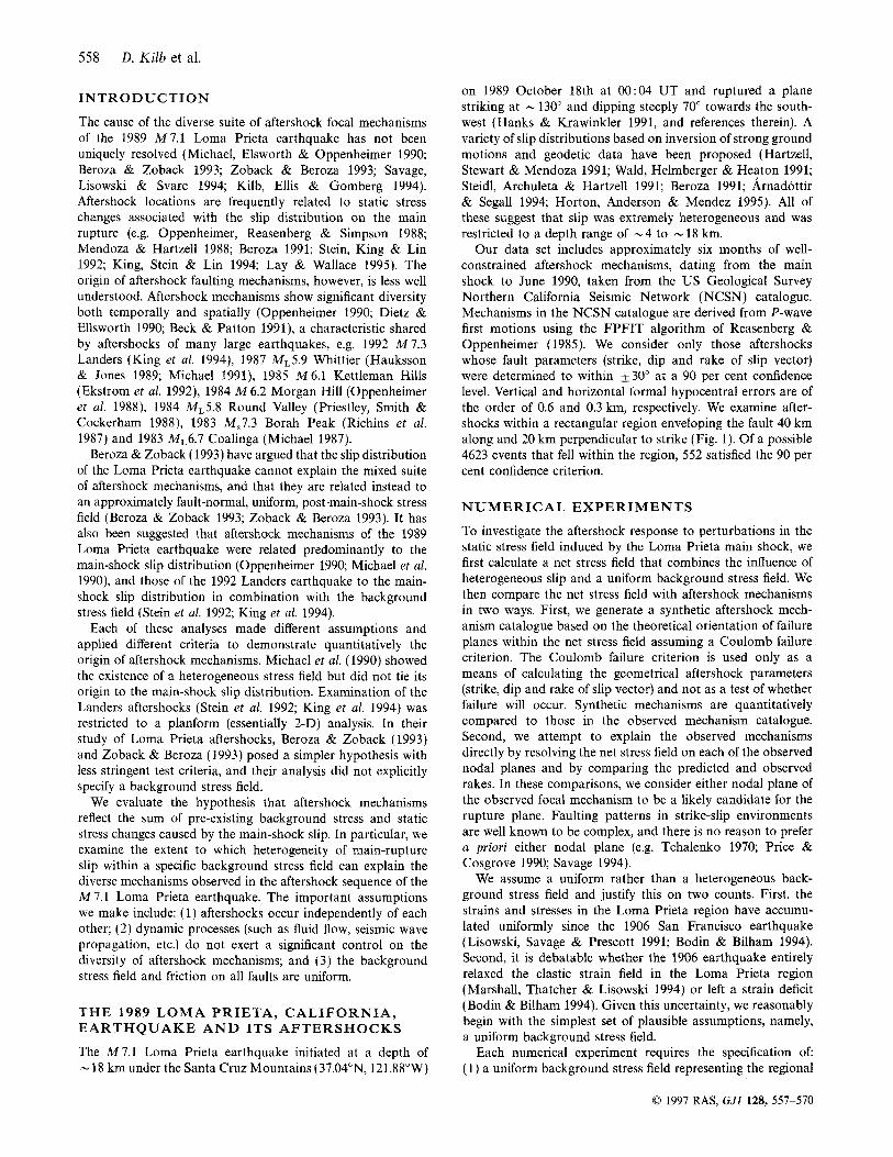
Figure 1. Map of the epicentral region of the California Loma Prieta earthquake showing the main-shock epicentre (star) and the 552 aftershock epicentres (circles) studied. A map view of the study area at the surface spans 60 km by 20 km (solid box) and a map view at 18 km depth (dashed box) are included to emphasize the effect of the 70" dip of the rupture plane.

stress field immediately prior to the main shock; (2) a main- shock rupture plane discretized into subfaults, each with an assigned slip vector obtained from a slip model; (3) aftershock locations; and (4) a constant frictional coefficient for all aftershock faults.

The numerical procedure includes the following steps. The stress field at a given aftershock location is calculated as the sum of the stress generated by the main-shock slip and the background stress field. We use a 3-D boundary-element algorithm (Gomberg & Ellis 1994) to calculate stress fields. Two possible conjugate failure planes are determined at each location consistent with a Coulomb failure criterion and a given frictional coefficient. If the frictional coefficient is zero, failure planes will correspond to the nodal planes of a single focal mechanism; otherwise, the failure planes correspond to two different focal mechanisms (Fig. 2). These synthetic mechanisms represent optimally oriented fault planes.

Synthetic and observed mechanisms are compared quantitatively using the normalized seismic consistency of Frohlich & Apperson (1992):

(1) II n = l cs= N

1 IIMij(n) II " = l

where Mij(n) in the nth normalized (geometric) moment tensor. A Cs value can be determined for two moment tensors

(a)

one focal mechanism

p=O

two possible

(b) conjugate failure planes

Figure 2. The generation of synthetic aftershock mechanisms involves the calculation of conjugate failure planes with a given frictional coefficient. (a) When the frictional coefficient is zero ( p = 0) conjugate failure planes and focal-mechanism nodal planes coincide, corresponding to one possible focal mechanism. (b) When the frictional coefficient is greater than zero ( p > O ) the predicted conjugate failure planes correspond to two possible focal mechanisms.

(N = 2) or a suite of mechanisms (N =number of tensors in the suite). Cs tends to zero in populations of diverse focal mechanisms and to one as mechanisms become similar to each other.

When using the Cs value to compare a single pair of synthetic and observed mechanisms, we choose the synthetic conjugate plane that best matches the datum. We assume that two focal mechanisms are indistinguishable from one another (a 'good'

0 1997 RAS, GJI 128, 557-510

560 D. Kilb et al.

fit) if Cs > 0.85. This value corresponds to a mismatch in strike, dip and rake of -30” (the maximum allowed uncertainty in our data set). In the direct comparison of the predicted and observed rakes, when stresses are resolved onto observed nodal planes, we regard a fit as successful if the match is within the rake uncertainty reported in the NCSN catalogue.

It is important to determine criteria for meaningful predictions to distinguish good fits from those obtained from a random sample. To accomplish this we determine how the percentage of successfully predicted aftershock mechanisms (Cs > 0.85) changes when using a temporally and spatially reordered observation catalogue (Appendix A). If the reordered results do not differ from the base results by more than 10 per cent, we infer that our results are not statistically significant.

B A C K G R O U N D D E F O R M A T I O N FIELDS

We use three different uniform background deformation fields. The first, D,, assumes right-lateral simple shear with a maximum shear orientation of 139”, parallel to the regional strike of the San Andreas fault but slightly clockwise of the 130” strike of the Loma Prieta section. This corresponds to a field in which the Loma Prieta section is a restraining bend, consistent with the local geomorphology (Anderson 1990) and structural geology (Aydin & Page 1984). We take the shear-strain rate to be 4 x yr-’ (Lisowski et al. 1991), giving a total fault-parallel shear since 1906 of 3.32 x The resultant displacement gradient tensor in a right-handed Cartesian coordinate system, X (north), Y (west), Z (up) is

1.64 1.43 0.00

D, = -1.89 -1.64 0.00 . ( 2 4 [ 0.00 0.00 o.oJ

[ 0.00 0.00

If we assume the Loma Prieta region shear velocity and density model of Beroza (1991; Table 2) and a Poisson’s ratio of 0.25, the corresponding Young’s modulus ranges between - 50 and 110 GPa. For our calculations we use a Young’s modulus of 70GPa and Poisson’s ratio of 0.25. The corresponding deviatoric stress tensor (MPa) is

0.92 -0.13 0.00

S1 = -0.13 -0.92 0.00 . ( 2b)

The second set of background deformation fields, DIB and D,,, is the same as the first but is scaled to induce average slips across the model Loma Prieta rupture plane of 1.1 and 0.93 m, equivalent to those inferred by Beroza (1991) and Horton et al. (1995), respectively. Thus, D,, = 3.6D1 and

D,, = 3.2D1. From the stress tensors corresponding to this larger-magnitude deformation field we estimate the maximum stress drop to be at most 3.3 MPa.

The third background deformation field, D,, based on the work of Zoback & Beroza (1993), assumes the maximum compressive stress is almost fault-normal, implying a frictional coefficient close to zero in order to induce slip on the main fault. The displacement gradient tensor and deviatoric stress tensor are, respectively,

0.513 -1.58 0.00

D, = [ -:::: 0.513 0.001 ,

[ 0.00 0.00 o.oJ ( 2 4

0.00 0.00

0.29 -0.88 0.00

S3 = -0.88 -0.29 0.00 . (2d)

D I S T R I B U T E D SLIP MODELS

We test the dependence of aftershock mechanisms on main- shock slip using two slip models with very different maximum slip amplitudes and slip gradients, those of Beroza (1991) and Horton (1995). Although the two slip models vary considerably in detail, the rupture geometries vary only slightly (Table 1, Figs 3a-b). Beroza (1991) derived his slip model from 20 strong-motion seismograms and a back-projection technique. Most of the slip occurs between 9 and 16 km depth (Fig. 3a). Horton’s (1995) model (Fig. 3b) was derived from geodetic and strong-motion data using a frequency-domain inversion technique (Mendez, Olson & Anderson 1990).

We also derive two free-slip models by letting the rupture plane slip as a stress-free boundary in response to the simple- shear background deformation fields, D, and D,. In each case, slip is distributed smoothly across the model rupture plane (Figs 3c-d). The corresponding stress fields differ only in their magnitude of maximum shear stress. One reflects a constant strain accumulation since 1906, a Young’s modulus of 70 GPa and Poisson’s ratio of 0.25. The other is larger and sufficient to induce the average observed slip across the Loma Prieta rupture, which implies a larger strain rate, a non-zero stress field in 1906, or a larger Young’s modulus.

For our study, the important differences between the Beroza and the Horton slip models include the location of the main- shock rupture plane and the amplitudes of slip and slip gradients. The fault planes defined by Beroza and Horton are not coincident (Table l), which alters the relative position of the aftershocks to the rupture plane. For each test we use the fault parameters that are consistent with the slip model being

Table 1. Rupture geometry’s of Beroza’s (1991) model and Horton’s (1995) model. The NW corner of the fault is with respect to the main-shock epicentre at (0,O).

0 1997 RAS, GJI 128, 557-570

Loma Prietak diverse aftershock mechanisms 561

Slip Model

Table 2. Slip model characteristics of Beroza's (1991) model, Horton's (1995) model and free-slip models driven with a background deformation proportional to the strain accumulation since 1906 (D1) and free slip but with a larger background deformation (DJ. We use M , = ~ A u . We computed the average slip (u) by first computing the average strike-slip and dip-slip displacements for the entire grid. We computed the total slip by taking the square root of the sum of the squares of these two average values. Hence, our values for M o are slightly lower than those reported by Beroza and Horton, who computed the total slip by adding each subfault total slip.

Average Maximum Maximum MO* Mw Total Slip Dip-Slip (m) Strike-Slip x1026

Beroza Horton

Free Slip (S 1) Free Slip (S2)

(m) (m) (dyne-cm) 1.1 4.4 5.5 2.0 6.8

0.93 1.3 1.3 2.0 6.8 0.29 0.17 0.42 0.54 6.4 1.0 0.15 I .4 2.0 6.8

Strike-slip Displacement (cm) Dip-slip Displacement (cm)

Nw SE NW SE (a)

(Max: 554, Min: -18) (Max: 437, Min: -15)

@fax: 131, Min: 6) (Max: 132, Min: -12)

(Max: 2. Min: -2) !Eza (Max: 15, Min: -1)

Figure 3. The dip (right) and strike (left) components of various slip models. Numbers indicate the range of slip magnitudes: positive is right- lateral and reverse motion for strike- and dip-slip respectively. (a) Beroza's (1991) model (strike-slip and dip-slip contour intervals are As = 100 and Ad = 50 respectively). (b) Horton's (1995) model (As = 10, Ad = 20). (c) A free-slip model driven with a background stress proportional to the strain accumulation since 1906 (As = 10, Ad = 0.5). (d) Same as (c) but larger background stress to induce the same average slip as Horton's (1995) and Beroza's (1991) models (As = 20, Ad = 2). The dip-slip component is not symmetrical for these free-slip models because of the 70" dip of the rupture plane in combination with the non-alignment between the orientation of the principal axes of the regional background stress field (139") and the strike of the rupture plane (130").

used. Although both models have approximately the same average slip (Table 2), the maximum slip amplitudes vary from 1.50 m (Horton) to 5.87 m (Beroza).

TEST OF ASSUMPTIONS

We assume that aftershock mechanisms are independent; that is, one aftershock does not influence another. To investigate this assumption, we pose the following questions. Do stress field perturbations from aftershocks contribute to the diversity in aftershock mechanisms? How large a volume does each

aftershock influence? If an aftershock significantly influences subsequent aftershock mechanisms, then a functional dependence between magnitude and mechanism diversity should be apparent. We address these questions by performing the three tests described below. A fourth test addresses the assumption that static stress dominates over time-varying processes.

Test 1: inclusion of aftershock rupture planes

We address these questions by making comparisons to reference calculations in which only the main-shock rupture

0 1997 RAS, GJI 128, 557-570

562 D. Kilb et al.

perturbs the background stress field. We then introduce 100 additional freely slipping faults placed at the first 100 aftershock locations. These locations are spatially well distributed throughout the region of aftershocks. We fix the strike and dip according to a randomly chosen nodal plane of the 100 observed focal mechanisms and assign a rupture dimension calculated for an assumed magnitude of 3.6 (0.42 km by 0.42 km; see below). The induced slip is as large as or larger than expected for the assumed magnitude. Also note that most aftershocks in our data set have a magnitude smaller than 3.6, thereby resulting in a conservative test. The change of the predicted fault parameters at the remaining 452 aftershock locations with and without the 100 additional faults provides a measure of their influence.

The resultant changes in strike, dip and slip-vector rake exceed their uncertainties only for event locations within 1 km of one of the 100 freely slipping faults. Recall, there are two conjugate planes corresponding to two possible mechanisms at each aftershock location. Of the two possible mechanisms, both conjugate planes show a significant change in the fault parameters for only 6 per cent of the aftershocks despite the exaggerated rupture dimension of the additional free-slipping faults. Because there is no a priori reason to choose one conjugate plane over the other, we conclude that aftershocks are independent, at least within the resolution of our data and analyses.

Test 2: dependence defined by influence zones and temporal sequence

If mechanism diversity reflects predominantly the interaction between aftershocks, we expect the mechanism diversity of independent aftershocks to differ from that of dependent aftershocks. We test this hypothesis by assuming a spherical zone of influence with radius R that is proportional to the rupture dimension, r. We classify an aftershock as independent if its influence zone is not overlapped by that of an earlier aftershock, regardless of the classification of the earlier aftershock (Fig.4). An aftershock that is overlapped by one or more influence zones of prior aftershocks is deemed to be dependent.

The seismic moment, M,, provides a measure of the rupture dimension and is estimated from catalogue local magnitudes, M,, according to the following relationships (Bakun, King & Cockerham 1986):

log(M,) = 1.2 M , + 17.0

log(Mo) = 1.5 M , + 16.0

for M , < 3.5,

for M , 2 3.5.

( 3 4

( 3b)

We estimate the rupture dimension, r, from M o , noting that M,=pAu (Aki & Richards 1980), in which the fault area (assumed circular) is A = nr'. The average rupture displacement, u, equals Aer (Ae is the failure strain or strain drop), and the rigidity is p = 3 x 1O'O Pa. Taking b e - 2 x we solve for the rupture dimension:

(4)

Cs values calculated for suites of mechanisms of independent or dependent aftershocks assuming an influence radius of R = r and R = 2 r (Table 3) indicate somewhat less diversity among dependent aftershocks than independent ones, although

Dependent

(b) f l o A i i i j ..:::::. 3 i i i i ;j , ili :.: , .::: :::::::..

Figure 4. Illustration of scheme to classify aftershocks as dependent (white) or independent (shaded). The numeric values indicate the time sequence, and circle radii are proportional to influence-zone dimen- sions. Thus in (a) only aftershocks 1 and 5 are independent, but in (b) aftershocks 1, 2 and 3 are independent.

by an amount that is within two standard deviations of the mean for a corresponding suite size (see Appendix A). Thus, this simple test supports the assumption that the interaction between aftershocks is not a dominant cause of the diversity among mechanisms.

Test 3: magnitude dependence

Another test of independence of aftershocks is based on the hypothesis that small-magnitude aftershocks are triggered by larger aftershocks (Mendoza & Hartzell 1988; King et al. 1994). We hypothesize that smaller, more numerous aftershocks have a greater probability of sampling varied stress fields than do larger aftershocks. If so, we should expect greater similarity in the mechanisms of large-magnitude aftershocks than for the small ones. We divide the mechanisms into magnitude bins, each containing 40 events, and determine a Cs value for each bin (Fig. 5a). We find no prominent magnitude dependence, which agrees with Michael et al. (1990).

Test 4: dynamic influences

Finally, we test the assumption that dynamic processes (such as fluid flow, post-seismic relaxation and seismic wave propagation) do not play a significant role in the diversity in aftershock mechanisms. If such processes are transient, com- mence with the main shock, and have time constants much shorter than the time span of our data, mechanism diversity might diminish with time. To test this hypothesis, we divide the mechanisms into temporal chronological bins of 40 events each and examine the Cs values for each bin. No time dependence in mechanism diversity is evident (Fig. 5b).

RESULTS OF NUMERICAL ANALYSES OF MECHANISM DIVERSITY

We show the ability of numerical experiments to predict, on a one-to-one basis, the observed focal mechanisms. First, we

0 1997 RAS, GJI 128, 557-570

Loma Prieta’s diverse aftershock mechanisms 563

Table 3. Consistency values for dependent and independent aftershocks.

(4 3.5 to 7.0 2.7 to 3.5 2.4 to 2.1

1.8 to 1.9 1.7 to 1.8 1.6 to 1.7

1.6 1.4 to 1.6 1.3 to 1.4 1.2 to 1.3

0 .o to 1.2

0 0.25

(b) Apr-Jun

APr Mar-Apr Dee-Mar Nov-Dec

Nov Oct29-Nov

E Oct 26-29 Oct 24-26 Oct 21-24 Oct 20-21 Oct 19-20 Oct 18-19

Oct 18

0 0.25 I I

0.5 0.75 1

cs

I

0.5

cs I I

0.75 1

Figure 5. (a) Consistency values, Cs, determined for magnitude bins containing -40 events each. (b) Consistency values, Cs, determined for increasing time intervals. There are approximately 40 mechanisms within each interval. No time dependence in mechanism diversity is evident.

compute a Cs value for each pair of observed and predicted mechanisms using the conjugate plane of the predicted mechanism that best matches the observation. Using Beroza’s slip model, background deformation D, , and a frictional coefficient of 0.6 for aftershock faults, 52 per cent of the predicted optimally oriented mechanisms agree (Cs > 0.85) with the observations (Fig. 6a, Method 1). Second, by directly resolving the stress field onto the aftershock plane, 41 per cent of the observed rakes agree (within the catalogue uncertainty) with predicted rakes (Fig. 6a, Method 2) . These two categories are not mutually exclusive and exhibit an overlap group consisting of aftershocks that are explained by both methods (i.e. aftershocks with optimally oriented observed nodal planes and rakes that are predicted from the resolved stress fields). By including this overlap, we are able to explain 61 per cent of aftershock mechanisms as a result of changes in the static stress field. Similar results hold for Horton’s slip model and the free-slip model regardless of the assumed background deformation model (Table 4). At best we are able to explain 69 per cent of the aftershocks (Horton’s slip model with background stress field &). The proportion of correctly predicted mechanisms is insignificantly different from selecting mechanisms from a randomly reordered catalogue (Fig. 6a, Method 1). (This randomization process is only appropriate for Method 1. It is not possible to do a similar randomization analysis for Method 2 due to the nodal-plane ambiguity and fixed strike and dip.)

It appears that individual mechanisms cannot be predicted correctly at a high level of significance. This result may reflect the uncertainty in the location of the aftershock. Our calculations show that regions exist where four different mechanism

types are possible within a 1 km3 volume. This same variability is exhibited in the observed mechanisms (Beroza & Zoback 1993; Oppenheimer 1990). Because the probable location error is - 1 km (Oppenheimer 1990), this mechanism variability must be investigated.

We attempt to incorporate location uncertainty by calculating synthetic mechanisms at six additional equally spaced positions within a 1 km3 volume surrounding the catalogue location. Of the 14 possible synthetic mechanisms (two mechanisms at each of the seven positions) for each aftershock location, we choose the mechanism that best matches the observation. Accounting for location uncertainty in this manner enables us to predict 92 per cent of the aftershock mechanisms (Fig. 6b). However, a comparison with a Cs value calculated for randomly reordered catalogues of observed mechanisms shows that our predictions are still no better than choosing mechanisms at random.

The uncertainty in predicted mechanisms associated with location uncertainty is compounded by their sensitivity to the assumed main-shock slip-distribution (Figs 7a-c). We show calculated horizontal grid maps of predicted slip vectors on conjugate failure planes at a depth of 11 km. Each of the two predicted conjugate slip vectors at a specific point corresponds to a different focal mechanism. The details of the resulting slip-vector patterns for each slip model are less important than are the clear differences between them. Similar differences are observed at other depths and in other fault parameters. The influence of the main-shock slip is clearly visible by the distinctly different pattern of predicted slip vectors each model shows near (within - 5 km of) the main-shock rupture where most of the aftershocks are located.

0 1997 RAS, GJI 128, 557-570

564 D. Kilb et al.

(a) Method 1

7 80 100

Method 1 and 2 .......... .......... B (DI) :_:;:;:;:;::;::::::: ..... ......,___

Percentage

100 0 20 40 60 80

Percentage

Method 1 and 2 (+1 km)

B (Dl)

H (01)

c] Method 1

2 B(D2) Overlap (Method 1 & 2)

H (D2)

F (W

B (D3)

0 20 40 60 80 100

100

Percentage

0 1997 RAS, GJI 128, 557-570

Loma Prieta's diverse aftershock mechanisms 565

Table 4. Percentage of aftershocks explained using different slip models and background stress fields. Method 1 tests for faults that are optimally oriented. Method 2 directly resolves the stress field onto the aftershock plane, and Method 1 & 2 represents faults that satisfied both methods.

Although useful prediction of individual focal mechanisms does not appear possible, we hypothesize that we may still learn something about the background stress field and main- shock slip distribution from a more gross-scale characteristic of the entire data set. In particular, we examine the diversity of the entire suite of 552 aftershock mechanisms. We measure the suite diversity by calculating a composite a value. For the observed suite of aftershock mechanisms, it is 0.459. a values for various slip and background stress field models range from 0.393 to 0.764 (Table 5, Fig. 8).

The suite diversity, a, for a given background stress field and treatment of location uncertainties is greatest for Beroza's slip model and smallest for the free-slip model. As we might expect, the heterogeneity of main-shock slip clearly influences the diversity of predicted aftershock mechanisms. The observed suite diversity agrees most closely with the synthetic suites generated using the lower-magnitude background stress field S, in conjunction with the slip models of Beroza and Horton. We discuss the implications of this in the next section.

Variation of the coefficient of friction, assuming it is identical for all faults, does not significantly alter the above results. Varying the frictional coefficients from 0.2 to 0.8 alters the predicted strikes, dips and slip vectors by less than 30" (which is within the bounds of the data uncertainty) and changes the Cs value from 0.426 (friction = 0.2) to 0.373 (friction = 0.8). Based on this research, we eliminate friction as a controlling parameter in the cause of mechanism diversity. Likewise, no systematic variation in focal mechanism diversity with depth or position along strike was apparent.

-

DISCUSSION

It is apparent that individual Loma Prieta aftershock mechanisms cannot be predicted successfully through a straight- forward analysis of static stress changes, because a similar degree of diversity can be obtained using a randomly temporally reordered aftershock catalogue. The combined uncertainties attached to the assumed main-shock slip distribution, locations of aftershocks, and the aftershock fault parameters are sufficient to explain this result. The sensitivity

of the resultant stress field to the slip distribution (Fig. 7) should be, by itself, a sufficient deterrent to attempt one-to- one comparisons of predicted and observed mechanisms. We note that these uncertainties are probably considerably smaller than for most earthquakes, since the Loma Prieta sequence is undoubtedly one of the most well constrained to date.

Another plausible contributing factor to our inability to make meaningful predictions (i.e. better than random) of individual mechanisms is that the background stress field is non-homogeneous, as might be expected in the tip-zone of the M,8.25 1906 earthquake (Bodin & Bilham 1994) and as suggested for the 1992 Landers earthquake (e.g. Stein et al. 1992; King et al. 1994). This is consistent with the requirement for a relatively large background stress field to induce sufficient average slip across a frictionless model Loma Prieta rupture plane. That is, it appears that the 1906 rupture did not completely relax elastic strains in this region so that the Loma Prieta rupture plane was pre-stressed, perhaps non-uniformly, to levels exceeding those expected, if we assume 83 years of strain accumulation.

Our results indicate that there may be more to learn from the diversity of the suite of well-constrained aftershock mechanisms than from individual mechanisms. The model that best predicts the observed suite diversity {Fig. 8) implies either a relatively low background stress field (corresponding to a complete stress drop in the Loma Prieta area after the 1906 earthquake), a heterogeneous slip distribution, or a suitable combination of the two. The former may imply a paradox, however, since the low background stress field cannot generate the observed average slip on a frictionless model fault plane. There are several possible explanations.

First, slip may not be driven by a uniform static stress field in the brittle crust. Stresses within the upper crust that ultimately drive displacement across the rupture may instead be generated by continuous plate motion across a shear zone within the lower crust or upper mantle (e.g. Savage & Burford 1970; Bilham & Bodin 1992; Molnar 1992). This process will yield a non-uniform distribution of stress in the upper crust, so that high levels of stress at lower-crustal depths manifest themselves as low levels of stress in the upper half of the upper

Figure 6. (a) The percentage of observed aftershock mechanisms consistent with those predicted. Top left, Method 1: the predicted strike, dip and rake correspond to optimally oriented faults consistent with the stress field. The vertical line denotes the percentage of aftershock mechanisms consistent with predicted optimally oriented faults based on a randomly reordered catalogue. Top right, Method 2: rakes are predicted according to the stress field resolved onto an observed nodal plane. Bottom, Methods 1 & 2 Aftershocks that are predicted by either or both methods 1 and 2. Regardless of slip model [B, H and F are the results for Beroza's (1991), Horton's (1995) and the free-slip models, respectively] and background deformation field (D1. D,, D3), we can only explain -61 per cent of the observed mechanism of interest. (b) As in (a), but accounting for location error (k 1 km).

Q 1997 RAS, GJI 128, 557-570

566 D. Kilb et al.

30 I I

I I 20

10

- 10

-20

--

(a) -20 0 20

Kilometers

30 1

20

10 E 3 g o 3 -10

-20 -: I

-30 ‘ I I f -20 0 !20

(c> Kilometers

crust (see also Bruhn & Schultz 1996). Thus, aftershocks within our study region may be sampling shear-stress levels that are nominal compared to the magnitude of deeper shear stresses that are ultimately responsible for driving most of the displacement across the main rupture.

Other possible explanations for the paradox include inappro- priate assumptions of main-shock fault orientation or homogeneity in both the initial background stress field and in fault properties. It is also feasible that the paradox can partially be explained by assuming a larger Young’s modulus. However, even the upper limit (1 10 GPa) will bring about only one-third of the necessary increase at best. Alternatively, this apparent paradox may imply that aftershocks are not simply controlled by static stress.

Another consideration is the validity of the 2-D Coulomb failure criterion, which is an empirical criterion based almost completely on uniaxial or triaxial laboratory experiments. At almost every point enveloping the Loma Prieta rupture, the

30

20

10

0

- 10

-20

-30 -20

(b) 0 20

Kilometers

Figure 7. (a) Predicted slip vectors using Beroza’s (1991) slip model in combination with a background stress field. Rakes of both predicted optimally oriented conjugate planes on horizontal inspection planes at a depth of 11 km. The line indicates the intersection of the rupture plane with the inspection plane. Most aftershocks at this depth are located within 5 km of the indicated rupture plane. Grid points are spaced at 2 km intervals. As distance from the fault increases, the slip vectors become quite uniform (look like continuous lines) and are consistent with the background stress field. (b) As is (a), but predicted using Horton’s (1995) slip model. (c) As is (a), but predicted for a free-slip model.

net change in stress is derived from 3-D deformation. Currently, no failure criterion predicts 3-D patterns, leaving us to incorporate a 2-D failure criterion. It is well known that faulting patterns in 3-D strains are more complex than in 2-D fields (Oertel 1965; Reches 1978; Reches & Dieterich 1983). It is thus possible that the inability to explain the aftershock mechanisms reflects the limitations of a 2-D failure criterion rather than the inadequacy of the static-stress hypothesis.

We also speculate that, as locations and mechanisms of aftershocks become better constrained, it may be possible to use these data as further constraints in the derivation of main- shock slip distribution. This is predicated, however, on our initial hypothesis that changes in the static stress field are responsible for the generation of aftershocks. It is possible that dynamic stresses or other time-dependent processes, rather than or in addition to static stresses, are responsible for the generation of aftershocks (Spudich et al. 1995).

Our results differ from those of Beroza & Zoback (1993)

0 1991 RAS, GJI 128, 551-570


Table 5. Cs values computed for a suite of 552 mechanisms. Background deformation D, is proportional to a strain accumulation since 1906; for background deformation DZ we increase the background stress to induce the observed average slip. Background deformation D3 assumes the maximum compressive stress is almost fault-normal.

and Zoback & Beroza (1993), which show that the aftershock mechanisms may be explained by an approximately fault- normal uniform stress field that represents the residual field after the main-shock rupture. They concluded that the main- shock rupture was an almost complete stress-drop event. Beroza & Zoback ( 1993) examined the traction change induced by the main shock across either of the two possible fault planes and determined whether or not it was of the correct sign to trigger the aftershocks (e.g. had a component in the same direction as the observed slip). A background stress field was

not explicitly specified. In our study, which differs from those of Zoback & Beroza (1993) and Beroza & Zoback (1993), the stress field prior to the main shock (e.g. Stein et al. 1992; King et al. 1994) and the stress produced by the main shock are explicitly specified. We illustrate the potential influence on the types of faulting mechanisms in the presence or absence of a background stress field (Figs 9a-b), and we also adopt more stringent criteria for judging the goodness of fit between predicted and observed mechanisms.

CONCLUSIONS

We have found that it is unproductive to make individual comparisons of observed focal mechanisms from the 1989 M 7.1 Loma Prieta earthquake with synthetic focal mechanisms derived from static-stress calculations and a Coulomb failure criterion (i.e. we obtain a comparable success in matching mechanisms using catalogues in which the aftershocks have been randomly reordered). This is probably due to the cumulative uncertainties in aftershock parameters, main-shock slip distribution, and assumed background stress field. We have shown that the post-main-shock static stress field is sensitive to the main-shock slip distribution on the rupture plane, so that significantly different focal mechanisms may be generated at a length scale shorter than reasonable aftershock location errors.

We are able to duplicate and explain the gross-scale mechanism diversity of the entire suite of aftershocks as a function of heterogeneous slip across the main-shock rupture and a relatively low-magnitude background stress field. This has the interesting consequence that the level of deviatoric stress in

H(D2j--)-I #??>,#,,,, ,//,/,,,,,,/,,/,/,,,,/, ,/,,/,,& I b 2

I 1

0 0.2 0.4 0.6 0.8 1

cs Figure 8. Cs values for a suite of 552 aftershock mechanisms for various slip models and background stress magnitudes. B, H and F are results for Beroza’s (1991), Horton’s (1995) and the free-slip models, respectively. Background deformation fields D,, Dz, D, correspond respectively to right-lateral simple shear accumulated since 1906, larger right-lateral simple shear scaled to induce an average total slip on the rupture plane, and an approximate fault-normal background stress field. The Cs values calculated for the observed mechanisms are shown by the solid bar (One standard deviation of +0.015). The vertical line represents the Cs value of the data.

0 1997 RAS, GJI 128, 557-570

568 D. Kilb et al.

30 1 1

"V

-20 20 A Kilometers

30

20

10

4- 6

3 E O

-10

-20

-30

-30 -20 -10 0 10 20 30 B Kilometers

Figure 9. (a) As is (7a), but predicted using Beroza's slip model with D, background deformation field. (b) As is (7a), but predicted using Beroza's slip model with no background stress field.

the upper crust prior to the main shock is insufficient to drive the main shock. We conclude by proposing that the origin of the variable aftershock mechanisms following the 1989 Loma Prieta earthquake is related to a combination of heterogeneous slip across the main rupture and a relatively low-level background stress.

ACKNOWLEDGMENTS

We are grateful for insightful comments by Andy Michael, David Oppenheimer and Steven Ward. Thanks also to Greg Beroza for his close reading, and very informative suggestions. We also thank our colleagues at the Center for Earthquake Research and Information for many critical discussions.

DK was supported by a US Geological Survey Graduate Fellowship. Additional support was provided by NSF award EAR-9219676 to ME. CERI Contribution number 292.

REFERENCES

Aki, K & Richards, P.G., 1980. Quantitative Seismology, W.H. Freeman & Co., New York, NY.

Anderson, R.S., 1990. Evolution of the northern Santa Cruz mountains by advection of crust past a San Andreas fault bend, Science,

Arnadbttir, T. & Segall, P., 1994. The 1989 Loma Prieta earthquake imaged from inversion of geodetic data, J . geophys. Res., 99,

Aydin, A. & Page, M.B., 1984. Diverse Pliocene-Quaternary tectonics in a transform environment, San Francisco Bay region, California, Geol. SOC. Am. Bull., 95, 1303-1317.

Bakun, W.H., King, G.C.P. & Cockerham, R.S., 1986. Seismic slip, aseismic slip, and the mechanics of repeating earthquakes on the Calaveras fault, California, in Earthquake Source Mechanics, pp. 195-207, Am. Geophys. Un, Washington, DC.

Beck, S.L. & Patton, H.J., 1991. Inversion of regional surface-wave spectra for source parameters of aftershocks from the Loma Prieta earthquake, Bull. seism. Soc. Am., 81, 1726-1736.

Beroza, G.C., 1991. Near-source modeling of the Loma Prieta earthquake: Evidence for heterogeneous slip and implications for earthquake hazards, Bull. seism. SOC. Am., 81, 1603-1621.

Beroza, G.C. & Zoback, M.D., 1993. Mechanism diversity of the Loma Prieta aftershocks and the mechanics of mainshock-aftershock interaction, Science, 259, 210-213.

Bilham, R. & Bodin, P., 1992. Fault zone connectivity; Slip rates on faults in the San Francisco Bay area, Science, 258, 281-284.

Bodin, P. & Bilham, R., 1994. Cumulative slip along the peninsular section of the San Andreas fault, California, estimated from two- dimensional boundary-element models of historical rupture, in US geol. Survey Professional Paper 1550-F, pp. F91LF101, ed. Simpson, R.W., Washington, DC.

Bruhn, R.L. & Schultz, R.A., 1996. Geometry and slip distribution in normal fault systems: Implications for mechanics and fault-related hazards, J. geophys. Res., 101, 3401-3412.

Dietz, L.D. & Ellsworth, W.L., 1990. The October 17, 1989, Loma Prieta, California earthquake and its aftershocks: geometry of the sequence from high-resolution locations, Geophys. Res. Lett., 17,

Ekstrom, G., Stein, R.S., Eaton, J.P. & Eberhart-Phillips, D., 1992. Seismicity and geometry of a 110-km-long blind thrust fault 1. The 1985 Kettleman Hills, California, earthquake, J . geophys. Res., 97,

Frohlich, C. & Apperson, D.K., 1992. Earthquake focal mechanisms, moment tensors, and the consistency of seismic activity near plate boundaries, Tectonics, 11, 279-296.

Gomberg, J. & Ellis, M., 1994. Topography and tectonics of the central New Madrid seismic zone: Results of numerical experiments using a three-dimensional boundary element program, J. geophys. Res.,

Hanks, T.C. & Krawinkler, H., 1991. The 1989 Loma Prieta Earthquake and its effects: introduction to the special issue, Bull. seism. Soc. Am., 81, 1415-1423.

Hartzell, S.H., Stewart, G.S. & Mendoza, C., 1991. Comparison of L1 and L2 norms in a teleseismic waveform inversion for the slip history of the Loma Prieta, California, Earthquake, Bull. seism. SOC. Am., 81, 1518-1539.

Hauksson, E. & Jones, L.M., 1989. The 1987 Whittier Narrows earthquake sequence in Los Angeles, Southern California: seismo- logical and tectonic analysis, J . geophys. Res., 94, 9569-9589.

Horton, S., Anderson, J.G. & Mendez, A,, 1995. Frequency-domain

249, 397-401.

21 835-21 855.

1417-1420.

4843-4864.

99, 20 299-20 310.

0 1997 RAS, GJI 128, 557-570


inversion for the character of rupture during the 1989 Loma Prieta, California earthquake using strong motion and geodetic observations, in U S geol. Survey Professional Paper 1550-A, ed. Spudich, P., Washington, DC.

Kilb, D., Ellis, M.A. & Gomberg, J., 1994. What induces the heterogeneous mechanisms of the 1989 Loma Prieta Earthquake?, EOS, Trans. Am. geophys. Un., 75, 439.

King, G.C.P., Stein, R.S. & Lin, J., 1994. Static stress changes and the triggering of earthquakes, Bull. seism. SOC. Am., 84, 935-953.

Lay, T. & Wallace, T.C., 1995. Modern Global Seismology, Academic Press, San Diego, CA.

Lisowski, M., Savage, J.C. & Prescott, W.H., 1991. The velocity field along the San Andreas fault in central and southern California, J. geophys. Res., 96, 8369-8389.

Marshall, G.A., Thatcher, W. & Lisowski, M., 1994. Resolution of fault slip along the 450-km-long rupture of the great 1906 San Francisco Earthquake, EOS, Trans. Am. geophys. Un., 75, 180.

Mendoza, C. & Hartzel, S.H., 1988. Aftershock patterns and main shock faulting, Bull. seism. SOC. Am., 78, 1438-1449.

Mendez, A.J., Olson, A.H. & Anderson, J.G., 1990. A norm mini- mization criterion for the inversion of earthquake ground motion, Geophys. J. Int., 102, 287-298.

Michael, A.J., 1987. Stress rotation during the Coalinga aftershock sequence, J. geophys. Res., 92, 7963-7979.

Michael, A.J., 1991. Spatial variations in stress within the 1987 Whittier Narrows, California, aftershock sequence: new techniques and results, J. geophys. Res., 96, 6303-6319.

Michael, A.J., Ellsworth, W.L. & Oppenheimer, D.H., 1990. Coseismic stress changes induced by the 1989 Loma Prieta, California earthquake, Geophys. Res. Lerr., 17, 1441-1444.

Molnar, P., 1992. Brace-Goetze strength profiles, the partitioning of strike-slip and thrust faulting at zones of oblique convergence, and the stress-heat flow paradox of the San Andreas Fault, in Fault Mechanics and Transport Properties of Rocks, pp. 435-459, eds Evans, B. & Wong, T.F., Academic Press Inc., San Diego, CA.

Oertel, G., 1965. The mechanism of faulting in clay experiments, Tectonophysics, 2, 343-393.

Oppenheimer, D., 1990. Aftershock slip behavior of the 1989 Loma Prieta, California Earthquake, Geophys. Res. Lett., 17, 1199-1202.

Oppenheimer, D.H., Reasenberg, P.A. & Simpson, R.W., 1988. Fault plane solutions for the 1984 Morgan Hill, California, earthquake sequence: Evidence for the state of stress on the Calaveras fault, J. geophys. Res.. 93, 9007-9026.

Price, N.J. & Cosgrove, J.W., 1990. Analysis of Geological Structures, Cambridge University Press, Cambridge.

Priestley, K.F., Smith, K.D. & Cockerham, R.S., 1988. The 1984 Round Valley, California earthquake sequence, J . Geophys., 95, 215-235.

Reasenberg, P. & Oppenheimer, D., 1985. FPFIT, FPPLOT and FPPAGE: FORTRAN computer programs for calculating and displaying earthquake fault-plane solutions, USGS Open-file report,

Reches, Z., 1978. Analysis of faulting in three-dimensional strain field, Tectonophysics, 47, 109-129.

Reches, Z. & Dieterich, J.H., 1983. Faulting of rocks in three- dimensional strain fields I. Failure of rocks in polyaxial, servo- control experiments, Tectonophysics, 95, 11 1-132.

Richins, W.D., Pechmann, J.C., Smith, R.B., Langer, C.J., Goter, S.K., Zollweg, J.E. & King, J.J., 1987. The 1983 Borah Peak, Idaho, earthquake and its aftershocks, Bull. seism. Sac. Am., 77, 694-723.

Savage, J.C., 1994. Evidence for near-frictionless faulting in the 1989 (M 6.9) Loma Prieta, California, earthquake and its aftershocks: Comment and Reply, Geology, 22, 278-280.

Savage, J.C. & Burford, R.O., 1970. Accumulation of tectonic strain in California, Bull. seism. SOC. Am., 60, 1877-1896.

Savage, J.C., Lisowski, M. & Svarc, J.L., 1994. Postseismic deformation following the 1989 (M = 7.1) Loma Prieta, California, earthquake, J. geophys. Res., 99, 13 757-13 765.

85-739, 109.

Spudich, P., Steck, L.K., Hellweg, M., Fletcher, J.B. & Baker, L.M., 1995. Transient stresses at Parkfield, California, produced by the M 7.4 Landers earthquake of June 28, 1992 Observations from the UPSAR dense seismograph array, J. geophys. Res., 100, 675-690.

Steidl, J.H., Archuleta, R.J. & Hartzell, S.H., 1991. Rupture history of the 1989 Loma Prieta, California, Earthquake, Bull. seism. SOC. Am.,

Stein, R.S., King, G.C.P. & Lin, J., 1992. Change in failure stress on the southern San Andreas fault system caused by the 1992 magnitude = 7.4 Landers earthquake, Science, 258, 1328-1332.

Tchalenko, J.S., 1970. Similarities between shear zones of different magnitudes, Geol. SOC. Am. Bull., 81, 1625-1640.

Wald, D.J., Helmberger, D.V. & Heaton, T.H., 1991. Rupture model of the 1989 Loma Prieta earthquake from the inversion of strong- motion and broadband teleseismic data, Bull. seism. SOC. Am., 81,

Zoback, M.D. & Beroza, G.C., 1993. Evidence for near-frictionless faulting in the 1989 (M 6.9) Loma Prieta, California, earthquake and its aftershocks, Geology, 21, 181-185.

81, 1573-1602.

1540-1572.

APPENDIX A: RANDOMIZATION TECHNIQUE A N D SUITE SIZE EFFECT ON Cs VALUES

To investigate the significance of fits between observed focal mechanisms and the corresponding synthetic focal mechanisms at a given aftershock location, we use a randomization technique. A synthetic reference mechanism based on Beroza’s 1991 slip model, background stress field S, and a frictional coefficient of 0.6 is estimated. A reference diversity value, Csref, is calculated for this synthetic mechanism and the observed focal mechanism. The percentage of aftershock mechanisms that are successfully predicted (Cs,, > 0.85) is determined. Next, at each aftershock location, a random diversity value is calculated using the reference synthetic mechanism and a randomly chosen observation. We repeat this randomization process 1000 times (1 104 mechanisms are possible assuming either plane of the 552 aftershocks to be a likely rupture plane) and at each aftershock location calculate an average randomized diversity value. This average Cs value is compared to the corresponding reference value Csref at each aftershock location. A difference exceeding one standard deviation between the two values at a majority of aftershock locations indicates that the similarity between the model prediction and observation could not be obtained by chance. As a more global check, we compare the overall percentage of aftershock mechanisms successfully predicted by the synthetic reference mechanisms with the overall percentage successfully predicted from the randomized set of observations. If these percentages are within one standard deviation ( < l o per cent) of each other, we infer that one-to-one comparisons of synthetic aftershock focal mechanisms with observed focal mechanisms are no better than random.

The Cs value is dependent on suite size. For example, with more independent events, it is likely that moment-tensor components will cancel, and thus a larger suite size results in a smaller Cs value. The expected value of Cs for two independent double-couple mechanisms is 0.68 i 0.18, whereas the distribution of Cs values for random suites of 552 mechanisms has a mean of 0.040 and a standard deviation of 0.014. The equation that approximately governs this behaviour is Cs z N - 0 . 5 ,

where N is the suite size. For the majority of the work presented in this paper, we

0 1997 RAS, GJI 128, 557-570

570 D. Kilb et al.

compare Cs values for suites of the same size. Only in our test of the interaction between aftershocks (Test 2) do we need to compare Cs values from two substantially different suite sizes. To do this we examine how much each value deviates from the mean Cs value (computed from different subsets of the

data set) for a similar suite size. For example, if suite size N1 is less than the mean by one standard deviation and suite size N 2 is greater than the mean two standard deviations, we infer that the second group contains a more similar group of mechanisms than the first group.

on the origin of diverse aftershock mechanisms …dkilb/papers/kilb_etal_1997.pdfon the origin of...

Documents