on the optimality of bank runs: comment on allen and gale1022143831151.pdf · on the optimality of...

The Geneva Papers on Risk and Insurance Theory, 28: 33–57, 2003c© 2003 The Geneva Association

On the Optimality of Bank Runs:Comment on Allen and Gale

MARGARITA SAMARTIN [email protected] Carlos III de Madrid, Departamento de Economıa de la Empresa, Calle Madrid 126,28903 Getafe, Spain

Received December 1, 1999; Revised February 28, 2002

Abstract

This paper presents a model consistent with the business cycle view of the origins of banking panics. As in Allenand Gale (1998), bank runs arise endogenously as a consequence of the standard deposit contract in a world withaggregate uncertainty about asset returns. The purpose of the paper is to show that Allen and Gale’s result aboutthe optimality of bank runs depends on individuals’s preferences. In a more general framework, considered in thepresent work, a laissez-faire policy can never be optimal, and therefore, regulation is always needed in order toachieve the first best. This result supports the traditional view that bank runs are costly and should be preventedwith regulation.

Key words: bank regulation, bank runs, deposit contracts, optimal risk sharing, suspension of convertibility

JEL Classification No.: G21, G28, D8

1. Introduction

The banking system has traditionally been vulnerable to the problem of bank runs, in whichmany or all depositors at a bank attempt to withdraw their funds simultaneously. If thesewithdrawals at a particular bank then spread across banks in the same region or countrythey may generate a banking panic. These financial crises are costly and are prevented withdifferent intervention measures.

Banking panics were common in the US and Europe prior to the 20th century. Suspensionof convertibility or central bank intervention were the usual tools to deal with panics.However, most of the regulatory systems that prevailed in the US and Europe until the1980s, evolved as a consequence of the financial crisis of the 1930s.1 The Great Depression(1929–1933) had an important impact on the financial system of the US2 and led to thecreation of the Federal Deposit Insurance Corporation. This institution insured deposits upto $2500. Deposit insurance3 was an excellent measure to eliminate runs and there was acalmer period after World War II. However, the market induced desintermediation of the1970s, in the face of inflation and nominal rigid interest rate ceilings, and the BankingDirectives in Europe generated a deregulation of the banking systems in the US and Europein the 1980s. The experience with bank deregulation has not been entirely pleasant. Many USSavings and Loans failed in the 1980s and some European countries have also experienced

34 SAMARTIN

problems in the 1990s. Furthermore, many emerging countries have had severe problemsin their banking systems in recent years. All this has led to a rethinking of the frameworkof banking regulation.

Theoretical research on banking theory has focused on analyzing the microeconomic roleof banks in the economy (e.g. Bryant [1980], Diamond and Dybvig [1983], Bhattacharyaand Gale [1987], Jacklin and Bhattacharya [1988], Chari and Jagannathan [1988], andAllen and Gale [1998]). This stream of research has approached banking panics throughtwo different types of models.

First, the models of pure panic runs comprise those models in which bank runs occuras random phenomena, with no correlation with other economic variables. Bryant [1980],followed by Diamond and Dybvig [1983], made a significant contribution by modeling thedemand for liquidity and the transformation service provided by banks. They demonstratedthat demand deposit contracts, which enable the transformation of illiquid assets into moreliquid liabilities, provide a rationale both for the existence of banks and for their vulner-ability to runs. The optimal contract yields a higher level of consumption for those whowithdraw early than the technological return. Bank runs, thus, take place when the idea ofdeposit withdrawals spills over economic agents (an essential point is that banks satisfy asequential service constraint, see Wallace [1988]). The model concludes that with no aggre-gate uncertainty, a suspension of convertibility policy eliminates the bank run equilibrium.Otherwise, a deposit insurance policy would be more effective. Diamond and Dybvig’smodel attracted severe criticisms (e.g., Gorton [1988]) for assuming that bank runs arerandom phenomena, and thus, uncorrelated with other economic variables. Gorton [1988],in an empirical study of bank runs in the US during the National Banking Era (1863–1913),found support for the notion that bank runs tended to occur after business cycle peaks.

Second, models of information-induced runs assert that bank runs occur due to the diffu-sion of negative information among depositors about a bank’s solvency, and therefore arenot the result of sunspots. These type of models is consistent with the business cycle view ofthe origin of panics (e.g., Jacklin and Bhattacharya [1988], Chari and Jagannathan [1988],and Allen and Gale [1998] among others). Jacklin and Bhattacharya [1988] examined therelative degrees of risk-sharing provided by bank deposit and traded equity contracts. Theyfocused on the relationship between the riskness of and information on the stream of returns,and the desirability of equity versus deposit contracts. They found that deposit contractstended to the better for financing low risk assets. Chari and Jagannathan [1988] drew onboth information-induced and pure panic runs models4 to study the effects of extra marketconstraints, such as suspension of convertibility on bank runs. They concluded that suchconstraints prevent bank runs and result in superior allocations. Despite the importance ofthis contribution, it raised considerable criticisms due to: (i) the ambiguous role of banks orany other financial intermediary in the model, (ii) assuming that individuals were risk neu-tral. An interesting addition to this literature is the recent paper by Allen and Gale [1998].In constrast to previous literature,5 which has focused mainly on modeling bank runs, thispaper analyzes the optimal intervention policy that should be implemented, if any, to dealwith panics. As in Diamond and Dybvig, individuals have corner preferences, that is, at date1, agents have realized utility for date 1 or date 2 consumption only. However, in this modelthe bank invests in a risky technology and individuals receive information about returns at

ON THE OPTIMALITY OF BANK RUNS 35

date 1. Bad information has then the power to precipitate a crisis. The paper shows thatunder certain circumstances, bank runs can achieve the first best outcome, as they allowefficient risk sharing among depositors and they allow banks to hold efficient portfolios.This result seems to contradict the traditional history of regulation, based on the premisethat banking panics are bad and should be eliminated. However, if there are liquidation costsor markets for risky assets are introduced, laissez-faire is no longer optimal, and centralbank intervention is needed to achieve the first best.

In the present paper it will be shown that even if there are no liquidation costs, a laissez-faire policy is not optimal, provided individuals’ preferences are smooth. The model pre-sented here is consistent with the business cycle view of the origins of banking panics. As inAllen and Gale [1998], banks operate in a competitive environment and so they offer depositcontracts that maximize the expected utility of the consumers. The behavior of the bankingindustry is thus represented by an optimal risk sharing problem. The paper considers twodifferent risk sharing problems: it is first assumed that banks can write contracts where theamounts individuals withdraw at each date can be made contingent on the return on the riskyasset. This problem provides a benchmark for optimal risk sharing. Secondly, and in linewith Allen and Gale’s paper, we consider a standard contract, which offers individuals fixedpayments at each date, and which is therefore by definition “non contingent”. In this secondcase, bank runs arise endogenously as a result of the negative signal which is observed bysome depositors in the interim period. However, the key difference with Allen and Gale[1998] is that in this paper individuals’ preferences are describable as smooth, that is, atdate 1 agents derive utility for consumption in both periods of their lives (although type-1agents derive relatively more utility for consumption in period 1 than type-2 agents). 6 Thisframework allows for total bank runs, as opposed to Allen and Gale [1998] where runs werealways partial. In their case, as type-1 agents derive only utility for consumption at date 1,being the only type-2 to stay the course would give the investor infinite returns when thelong-term asset return is close to zero. By contrast, in this model, as both types of agentsconsume in the two periods, the lone type-2 simply obtains a somewhat larger share of avery small pie. Type-2 agents are then better off by running on the bank. However, if alltype-2 agents run, they would consume too much at date 1 relatively to the first best. Thebank can then restrict payments at date 1 if the bank’s return is very low, and this will reducethe amount of first period cash that type-2 individuals obtain by imitating type-1s to thepoint to which they are willing to follow the type-2 plan.

The contribution of the present paper is in this sense to show that Allen and Gale’s resultabout the optimality of bank runs depends on individuals’ preferences. In a more generalframework, considered in the present work, standard contracts and bank runs can neverachieve the first best outcome, unless payments are restricted at date 1. This result supportsthe traditional view that bank runs are costly and should be prevented with regulation.

The structure of the paper is as follows: The basic framework of the model is presented inSection 2. As mentioned above the behavior of the banking industry is characterized by theoptimal, incentive compatible risk sharing problem. Two different risk sharing problems areconsidered. In Subsection 2.1 we assume that the optimal allocation can be made contingenton the return on the risky asset, and is considered as the benchmark case. In Subsection 2.2we consider the case in which banks offer standard contracts, that are not contingent on

36 SAMARTIN

the return on the risky asset. However, individuals can observe this return and make theirwithdrawal decision conditional on it. It is shown that when individuals’ preferences aresmooth, standard contracts and bank runs can never achieve optimal risk sharing unless asuspension of payments policy is implemented. Finally, Section 3 concludes the paper.

2. The model

There is an economy going through a sequence of three periods (T = 0, 1, 2) and onegood per period. There are two types of assets: a safe asset and a risky one. The safe assettransforms one unit of the consumption good at T into one unit of the consumption good atT +1. It can be thought of as a storage technology. The risky asset transforms one unit of theconsumption good at T = 0 into R units of the consumption good at T = 2, and where Ris a nonnegative random variable with a probability density function f (R). For simplicity,it is assumed that the long-term technology cannot be liquidated early, or equivalently, nocosts for early withdrawals are assumed.

On the household side of the economy there is a continuum of ex-ante identical agents,who are endowed with k0 units of the good at T = 0 and that maximize expected utility ofconsumption. They are subject at T = 1 to a privately observed uninsurable risk of being ofeither of two types. They can be of type-1 with probability t1 or of type-2 with probabilityt2. The difference between types is that type-1 agents derive relatively more utility fromconsumption in the first period with respect to type-2 agents. The following form for theutility function is assumed:

U j (c1 j , c2 j , ρ j ) = ρ j ln c1 j + (1 − ρ j ) ln c2 j (1)

where j = type = 1, 2. For simplicity, the following values for the parameter ρ j will beconsidered: ρ1 = ρ > 0.5, ρ2 = 1 − ρ < 0.5 and 0 ≤ ρ2 ≤ ρ1 ≤ 1. Note that Allen andGale’s results can simply be derived as extreme cases corresponding to ρ1 = 1 and ρ2 = 0.

At T = 1 depositors observe a signal, which predicts with perfect accuracy the value ofR that will be realized at date 2.

It is finally assumed no aggregate uncertainty so that with probability 1 a fraction t1 ofconsumers are of type-1 and a fraction t2 of type-2 and also the expected return is greaterthan one (E[R] > 1), that is, the risky asset is more productive than the safe one.

The following notation will be used throughout the paper:

µ = 1 − ρ

ρ, t1m = t1 + t2µ

1 + µ, t2m = t2 + t1µ

1 + µ(2)

and where 0 < µ < 1 and t1m + t2m = t1 + t2 = 1.

2.1. The optimal incentive-compatible risk sharing problem

As a benchmark case, it is first assumed that banks can write contracts where the amountthat is withdrawn at each date can be made contingent on the random return (R). Thedeposit contract can be represented by the functions c1 j (R),c2 j (R)(i = 1, 2), which specifyconsumption at dates 1 and 2 for a type j consumer.


The optimal risk sharing problem can be written as follows:

maxci j ,k1,k2

{ER

[t1U 1(c11(R), c21(R), ρ1) + t2U 2(c12(R), c22(R), ρ2)

]}(3)

s.t. k1 + k2 ≤ k0

t1c11(R) + t2c12(R) ≤ k1 (4)

t1[c21(R) + c11(R)] + t2[c22(R) + c12(R)] ≤ k1 + k2 R

U j (c1 j (R), c2 j (R), ρ j ) ≥ [U j (δ j c1i (R), (1 − δ j )c1i (R) + c2i (R), ρ j )](5)

for i �= j ; i, j = 1, 2; 0 ≤ δ j ≤ 1

where c1 j (R) represents consumption at time T = 1 for a type j agent, c2 j (R) consumptionat time T = 2 for a type j agent, k1 is the investment in the safe asset at T = 0 and k2 isthe investment in the risky asset at T = 0. The first constraint states that the total amountinvested must be less or equal to the amount deposited. The second constraint says that theinvestment in the safe asset should be enough to cover consumption at date 1. The third onerepresents the fact that the investment in the risky asset plus the amount of the safe one thatis left over from period one should be enough to cover consumption at date 2, that is:7

t1c21(R) + t2c22(R) ≤ k2 R + [k1 − t1c11(R) − t2c12(R)] (6)

The last two constraints are incentive compatibility constraints. In the case of a type-2 agent, incentive compatibility requires that the utility obtained from the consumptionbundle the individual receives if he is honest (c12(R), c22(R)), should be at least as largeas the utility obtained by lying and behaving like a type-1 agent, that is, obtaining theconsumption bundle (c11(R), c21(R)) and then reinvesting his first period consumption inthe storage technology in the optimal way for him. This means consuming δ2c11(R) in thefirst period and (1 − δ2)c11(R) + c21(R) in the second period. The same for type-1 agents.8

However, in solving the optimal risk sharing problem, the incentive compatibility con-straints can be dispensed with.9 The problem is solved subject to the three constraints andit can be shown that the incentive constraints are always satisfied. The following result isobtained:

Theorem 1: The solution [k1, k2, ci j (R)], to the optimal risk sharing problem is charac-terized by the following conditions:

if r ≤ 1 (case 1)

c11(R) = c22(R) = 1

1 + µ

k1

t1m[t1m + r t2m]

(7)c21(R) = c12(R) = µc11(R)

if r > 1 (case 2)

c11(R) = 1

1 + µ

k1

t1mc12(R) = µc11(R)

(8)c22(R) = rc11(R) c21(R) = µc22(R)

38 SAMARTIN

and k1, k2, the values that maximize the following expression:

maxk1,k2

[ ∫ 1

0U ∗(1) f (r ) dr

t2m

t1m

k1

k2+

∫ ∞

1U ∗(2) f (r ) dr

t2m

t1m

k1

k2

](9)

s.t. k1 + k2 = k0 (10)

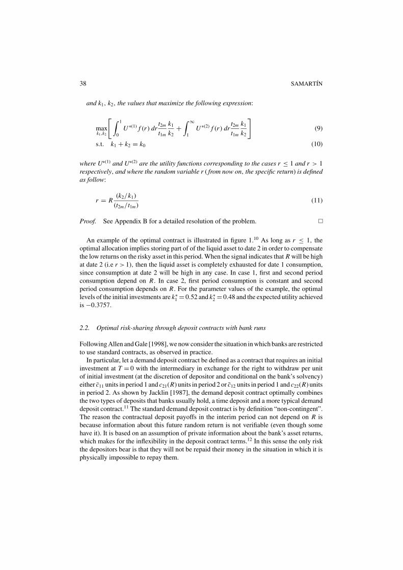
where U∗(1) and U∗(2) are the utility functions corresponding to the cases r ≤ 1 and r > 1respectively, and where the random variable r ( from now on, the specific return) is definedas follow:

r = R(k2/k1)

(t2m/t1m)(11)

Proof. See Appendix B for a detailed resolution of the problem.

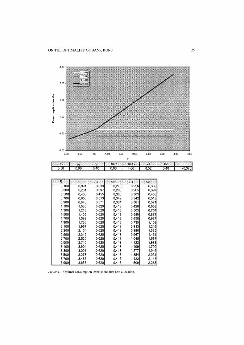
An example of the optimal contract is illustrated in figure 1.10 As long as r ≤ 1, theoptimal allocation implies storing part of of the liquid asset to date 2 in order to compensatethe low returns on the risky asset in this period. When the signal indicates that R will be highat date 2 (i.e r > 1), then the liquid asset is completely exhausted for date 1 consumption,since consumption at date 2 will be high in any case. In case 1, first and second periodconsumption depend on R. In case 2, first period consumption is constant and secondperiod consumption depends on R. For the parameter values of the example, the optimallevels of the initial investments are k∗

1 = 0.52 and k∗2 = 0.48 and the expected utility achieved

is −0.3757.

2.2. Optimal risk-sharing through deposit contracts with bank runs

Following Allen and Gale [1998], we now consider the situation in which banks are restrictedto use standard contracts, as observed in practice.

In particular, let a demand deposit contract be defined as a contract that requires an initialinvestment at T = 0 with the intermediary in exchange for the right to withdraw per unitof initial investment (at the discretion of depositor and conditional on the bank’s solvency)either c11 units in period 1 and c21(R) units in period 2 or c12 units in period 1 and c22(R) unitsin period 2. As shown by Jacklin [1987], the demand deposit contract optimally combinesthe two types of deposits that banks usually hold, a time deposit and a more typical demanddeposit contract.11 The standard demand deposit contract is by definition “non-contingent”.The reason the contractual deposit payoffs in the interim period can not depend on R isbecause information about this future random return is not verifiable (even though somehave it). It is based on an assumption of private information about the bank’s asset returns,which makes for the inflexibility in the deposit contract terms.12 In this sense the only riskthe depositors bear is that they will not be repaid their money in the situation in which it isphysically impossible to repay them.


Figure 1. Optimal consumption levels in the first best allocation.

40 SAMARTIN

That is, at T = 0 or ex-ante period, individuals deposit their k0 units of endowment inthe bank and are offered a menu of contracts, where they receive a fixed payment at date 1and a random one at date 2. The second period random payment will depend on the randomreturn R. This uncertain second period return reflects the fact that having invested in a riskyasset the bank may not be able to make its promised payments at date 2. In this situation,when the bank is restricted to use a standard contract, bank runs will become a possibility.It will be denoted by 0 ≤ α(R) ≤ t2 the fraction of type-2 agents that choose to run, orequivalently, that demand the type-1 contract when the value of R becomes sufficientlysmall (that is, when their incentive compatibility constraint is no longer satisfied). Let α(R)be defined as follows:

α(R)

= 0 if (1 − ρ) ln c12(R) + ρ ln c22(R) ≥ (1 − ρ) ln [δ2c11(R)]

+ ρ ln [(1 − δ2)c11(R) + c21(R)]

> 0 otherwise

(12)

Whenever a run occurs all available funds will be divided pro rata in proportion to claims(as in Allen and Gale [1998], we do not assume a sequential service constraint).

The bank chooses a portfolio k1, k2, the consumption functions c1 j (R), c2 j (R)( j = 1, 2),the deposit parameters c1 j , c2 j and the withdrawal function α(R) that maximizes the fol-lowing expression:

max{

ER

[t1U 1(c11(R), c21(R), ρ1) + t2U 2(c12(R), c22(R), ρ2)

]}(13)

s.t. k1 + k2 ≤ k0 (a)

[t1 + α(R)]c11(R) + [t2 − α(R)]c12(R) ≤ k1 (b)

[t1 + α(R)](c21(R) + c11(R)) + [t2 − α(R)][c22(R) + c12(R)] (c)

≤ k1 + k2 R

∀ 0 ≤ δ2 ≤ 1

(1 − ρ) ln c12(R) + ρ ln c22(R) ≥ (1 − ρ) ln [δ2c11(R)]

+ ρ ln [(1 − δ2)c11(R) + c21(R)] (d)

∀ 0 ≤ δ1 ≤ 1

ρ ln c11(R) + (1 − ρ) ln c21(R)

≥ ρ ln [δ1c12(R)] + (1 − ρ) ln [(1 − δ1)c12(R) + c22(R)] (e)

if 0 < α(R) < t2(1 − ρ) ln c12(R) + ρ ln c22(R)

= (1 − ρ) ln [δ2c11(R)] + ρ ln [(1 − δ2)c11(R) + c21(R)] (f)

if c11(R) < c11

[t1 + α(R)]c11(R) + [t2 − α(R)]c12(R) ≤ k1 (g)

c1 j (R) ≤ c1 j (h)

0 ≤ α(R) ≤ t2 (i)

(14)


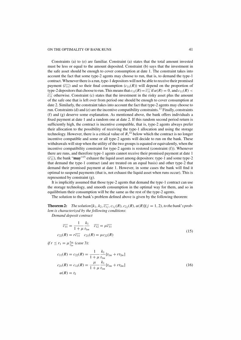
Constraints (a) to (e) are familiar. Constraint (a) states that the total amount investedmust be less or equal to the amount deposited. Constraint (b) says that the investment inthe safe asset should be enough to cover consumption at date 1. The constraint takes intoaccount the fact that some type-2 agents may choose to run, that is, to demand the type-1contract. Whenever there is a run, type-1 depositors will not be able to receive their promisedpayment (c11) and so their final consumption (c11(R)) will depend on the proportion oftype-2 depositors that choose to run. This means that c11(R) = c11 if α(R) = 0, and c11(R) <

c11 otherwise. Constraint (c) states that the investment in the risky asset plus the amountof the safe one that is left over from period one should be enough to cover consumption atdate 2. Similarly, the constraint takes into account the fact that type-2 agents may choose torun. Constraints (d) and (e) are the incentive compatibility constraints.13 Finally, constraints(f) and (g) deserve some explanation. As mentioned above, the bank offers individuals afixed payment at date 1 and a random one at date 2. If this random second period return issufficiently high, the contract is incentive compatible, that is, type-2 agents always prefertheir allocation to the possibility of receiving the type-1 allocation and using the storagetechnology. However, there is a critical value of R,14 below which the contract is no longerincentive compatible and some or all type-2 agents will decide to run on the bank. Thesewithdrawals will stop when the utility of the two groups is equated or equivalently, when theincentive compatibility constraint for type-2 agents is restored (constraint (f)). Wheneverthere are runs, and therefore type-1 agents cannot receive their promised payment at date 1(c11), the bank “may”15 exhaust the liquid asset among depositors: type-1 and some type-2that demand the type-1 contract (and are treated on an equal basis) and other type-2 thatdemand their promised payment at date 1. However, in some cases the bank will find itoptimal to suspend payments (that is, not exhaust the liquid asset when runs occur). This isrepresented by constraint (g).

It is implicitly assumed that those type-2 agents that demand the type-1 contract can usethe storage technology, and smooth consumption in the optimal way for them, and so inequilibrium their consumption will be the same as the rest of the type-2 agents.

The solution to the bank’s problem defined above is given by the following theorem:

Theorem 2: The solution [k1, k2, c1 j , c1 j (R), c2 j (R), α(R)]( j = 1, 2), to the bank’s prob-lem is characterized by the following conditions:

Demand deposit contract

c11 = 1

1 + µ

k1

t1mc12 = µc11

(15)c22(R) = rc11 c21(R) = µc22(R)

if r ≤ r1 = µ t1mt2m

(case 3):

c11(R) = c22(R) = 1

1 + µ

k1

t1m[t1m + r t2m]

c21(R) = c12(R) = µ

1 + µ

k1

t1m[t1m + r t2m] (16)

α(R) = t2

42 SAMARTIN

if r1 < r < 1 (case 2):

c11(R) = c22(R) = k1

t1 + α(R) + (t2 − α(R))µc12(R) = c21(R) = µc11(R) (17)

α(R) = 1

2

1 + µ

1 − µ

[t2m − t1m + t1m − t2mr

t1m + t2mr

]< t2

if r ≥ 1 (case 1):

c11(R) = c11 c12(R) = c12

c22(R) = rc11 c21(R) = rc22 (18)

α(R) = 0

and k1, k2, the values that maximize the following expression:

maxk1,k2

[ ∫ r1

0U ∗(1) f (r ) dr

t2m

t1m

k1

k2+

∫ 1

r1U ∗(2) f (r ) dr

t1m

t2m

k1

k2

+∫ ∞

1U ∗(3) f (r ) dr

t1m

t2m

k1

k2

](19)

s.t k1 + k2 = k0 (20)

Proof. See Appendix C for a detailed resolution of the problem.

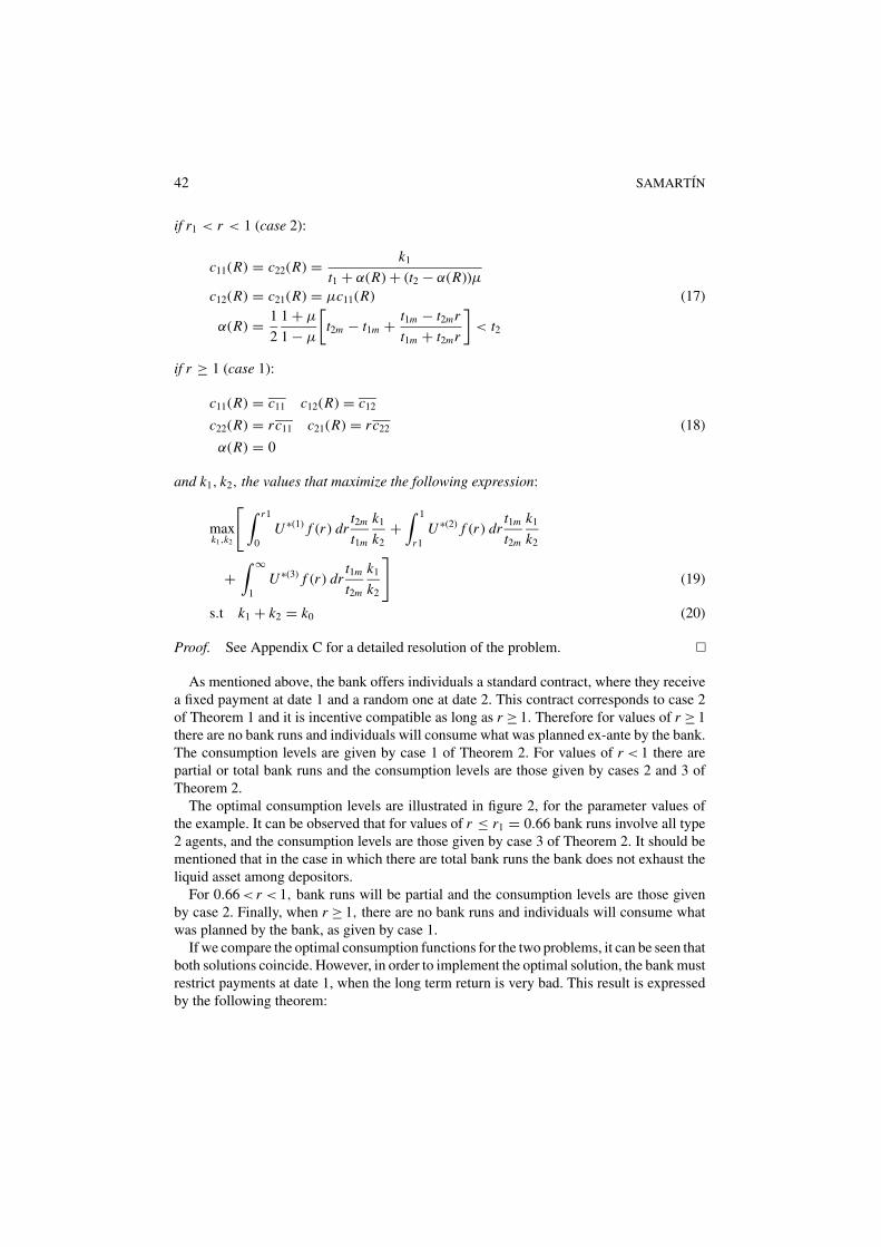
As mentioned above, the bank offers individuals a standard contract, where they receivea fixed payment at date 1 and a random one at date 2. This contract corresponds to case 2of Theorem 1 and it is incentive compatible as long as r ≥ 1. Therefore for values of r ≥ 1there are no bank runs and individuals will consume what was planned ex-ante by the bank.The consumption levels are given by case 1 of Theorem 2. For values of r < 1 there arepartial or total bank runs and the consumption levels are those given by cases 2 and 3 ofTheorem 2.

The optimal consumption levels are illustrated in figure 2, for the parameter values ofthe example. It can be observed that for values of r ≤ r1 = 0.66 bank runs involve all type2 agents, and the consumption levels are those given by case 3 of Theorem 2. It should bementioned that in the case in which there are total bank runs the bank does not exhaust theliquid asset among depositors.

For 0.66 < r < 1, bank runs will be partial and the consumption levels are those givenby case 2. Finally, when r ≥ 1, there are no bank runs and individuals will consume whatwas planned by the bank, as given by case 1.

If we compare the optimal consumption functions for the two problems, it can be seen thatboth solutions coincide. However, in order to implement the optimal solution, the bank mustrestrict payments at date 1, when the long term return is very bad. This result is expressedby the following theorem:


Figure 2. Optimal consumption levels with the standard contract.

44 SAMARTIN

Theorem 3: Assuming the support of R contains zero, then a banking system subject toruns cannot achieve first-best efficiency using a standard contract unless a suspension ofconvertibility policy is adopted.

Proof. As mentioned above, the bank offers individuals a standard contract which cannotbe made contingent on the risky return. For values of the specific return higher or equalto one (r ≥ 1), the contract is incentive compatible and there are no runs (α(R) = 0). Inthis case, the consumption functions coincide with those obtained in the first best case(case 2 of Theorem 1). For values of the specific return r1 < r < 1, the contract is no longerincentive compatible and there would be partial bank runs, involving only a fraction oftype-2 consumers (0 < α(R) < t2). It can be shown that substituting this value α(R), in theexpression for c11(R) corresponding to this case, it is obtained that c11(R) = 1

1+µk1t1m

[t1m +r t2m] and again these consumption functions coincide with the ones obtained in the first bestcase (case 1 of Theorem 1). Finally, for very low values of the specific return, r ≤ r1, alltype-2 agents will decide to run on the bank (α(R) = t2). In this case, the bank can implementthe first best allocation by suspending payments at date 1. This is the main difference withrespect to Allen and Gale’s results. In their case, due to the corner preference assumption,bank runs were always partial. As long as there is a positive value of the risky asset, theremust be a positive fraction of late consumers who wait until the last period, (p. 1259).16

In the numerical example the optimal levels of the initial investments are k∗1 = 0.52 and

k∗2 = 0.48 and the expected utility achieved with a standard contract is −0.3757.

The above result shows that Theorem 2 of Allen and Gale’s paper is not robust, andtherefore, it provides a rationale for banking regulation. In this sense, a suspension of con-vertibility policy, that restricts payments at date 1, would implement the first-best. Paymentsin the first period would be restricted to a level of k < k1, where k = 1

1+µk1t1m

[t1m + r t2m].17

3. Concluding remarks

The motivation of this paper has been to show that Allen and Gale’s result is not robust:In Theorem 2 of their paper they show that a standard demand deposit contract, which willlead to bank runs in some states of the world, achieves optimal risk sharing. However, ifthere are liquidation costs or markets for risky assets are introduced, then bank runs are nolonger optimal. Allen and Gale consider a particular characterization of preferences, wherethe so called type-1 depositors derive only utility for consumption in period 1 and type-2depositors derive utility for consumption in period 2. This paper extends the above model byconsidering a more general, and realistic, preference structure, in which individuals deriveutility for consumption in both periods of their lives, although type-1 agents derive relativelymore utility for consumption in period 1 with respect to type-2 agents. It is shown that inthis more general framework, even if there are no liquidation costs, standard contracts andbank runs can never achieve the first best outcome, unless a suspension of convertibilitypolicy is implemented.

The more general preference structure considered in the present work allows for totalbank runs and this is the main difference with respect to Allen and Gale’s model, where bank


runs were always partial. In their case, as type-1 agents received nothing at date 2, being theonly type-2 to stay the course would give the investor infinite returns when the long-termasset return is close to zero. By contrast, in this model, as type-1 agents are supposed toreceive some cash at date 2, the lone type-2 simply obtains a somewhat larger share of avery small pie. Type-2 agents are then better off by running on the bank. However, if alltype-2 agents run, they would consume too much at date 1 relatively to the first best. Thebank can then suspend convertibility if the bank’s return is very low, and this will reducethe amount of first period cash that type-2 individuals obtain by imitating type-1s to thepoint to which they are willing to follow the type-2 plan.

The contribution of the paper is in this sense to show that there are no positive aspects toa crisis, that is, bank runs are always costly and should be prevented with regulation.

Appendix A: Incentive compatibility constraints

In the optimal incentive risk-sharing problem defined in Subsection 2.1, it is assumedthat the realization of the timing of the consumption needs is private information of theconsumer. Given this information asymmetry, an allocation can only be implemented if itis incentive compatible, that is, if it gives no consumer an incentive to lie or deviate aboutwhat he actually wants to consume. In the case of a type 2 agent, incentive compatibilityrequires that the utility obtained from the consumption bundle he receives if he is honest(c12(R), c22(R)), should be at least as large as the utility obtained by lying and behavinglike a type 1 agent, that is, obtaining the consumption bundle (c11(R), c21(R)) and thenreinvesting his first period consumption in the storage technology in the optimal way forhim. If he reinvested part of his first period allocation (c11(R)) in this storage technology, hisoptimal consumption levels in both periods c∗2

1 (R), c∗22 (R) are the solution to the following

problem:

maxc1(R)·c2(R)

{(1 − ρ) ln c1(R) + ρ ln c2(R)} (21)

s.t. c1(R) ≤ c11(R) (22)

c2(R) = (c11(R) − c1(R)) + c21(R)

which yields:

(a) c∗21 (R) = c11(R) c∗2

2 (R) = c22(R) if µ > c11(R)c21(R)

(b) c∗1µ

1 (R) = (c11(R)+c21(R))µ1+µ

c∗22 (R) = c11(R)+c21(R)

1+µif µ ≤ c11(R)

c21(R)

(23)

The incentive compatibility constraint for a type-2 agent is then:

(1 − ρ) ln c12(R) + ρ ln c22(R) ≥ (1 − ρ) ln c∗21 (R) + ρ ln c∗2

2 (R) (24)

The incentive compatibility constraint for a type-1 agent is obtained in a similar way, andwould be:

ρ ln c11(R) + (1 − ρ) ln c21(R) ≥ ρ ln c∗11 (R) + (1 − ρ) ln c∗1

2 (R) (25)

46 SAMARTIN

where

(a) c∗11 (R) = c12(R) c∗1

2 (R) = c22(R) if µ < c22(R)c12(R)

(b) c∗11 (R) = c12(R)+c22(R)

1+µc∗1

2 (R) = (c12(R)+c22(R))µ1+µ

if µ ≥ c22(R)c12(R)

(26)

Appendix B: Optimal incentive compatible risk-sharing problem

The first best allocation is obtained as a solution to the following problem:

maxci j ,k1k2

{ER

[t1U 1(c11(R), c21(R), ρ1) + t2U 2(c12(R), c22(R), ρ2)

]}(27)

s.t. k1 + k2 ≤ k0

t1c11(R) + t2c12(R) ≤ k1 (28)

t1[c21(R) + c11(R)] + t2[c22(R) + c12(R)] ≤ k1 + k2 R


2 (R)(29)


2 (R)

and where c∗ ji , (i, j = 1, 2) were defined in the previous section. However, in solving the

optimal risk-sharing problem the incentive compatibility constraints can be dispensed with.The problem is solved subject to the three constraints and it can be shown that the first-bestsolution is always incentive compatible. For each value of R the consumption levels ci j (R)solve the problem:

maxci j ,k1k2

{ER

[t1U 1(c11(R), c21(R), ρ1) + t2U 2(c12(R), c22(R), ρ2)

]}(30)

s.t. t1c11(R) + t2c12(R) ≤ k1

t1[c21(R) + c11(R)] + t2[c22(R) + c12(R)] ≤ k1 + k2 R (31)

The Lagrangian is formed by using the lagrangian multipliers λ1 and λ2 of the first tworesource constraints.

The Kuhn-Tucker conditions are:

t1ρ1

c11(R) − λ1t1 − t1λ2 = 0 if c11(R) > 0 (a)

t1(1 − ρ) 1c21(R) − t1λ2 = 0 if c21(R) > 0 (b)

t2(1 − ρ) 1c12(R) − λ1t2 − t2λ2 = 0 if c12(R) > 0 (c)

t2ρ1

c22(R) − t2λ2 = 0 if c22(R) > 0 (d)

k1 − t1c11(R) − t2c12(R) = 0 if λ1 > 0 (e)

k1 + k2 R − t1[c11(R) + c21(R)] − t2[c12(R)

+ c22(R)] = 0 if λ2 > 0 (f)

(32)


Let

µ = 1 − ρ

ρ; t1m = t1 + t2µ

1 + µ; t2m = t2 + t1µ

1 + µ(33)

and

r = R(k2/k1)

(t2m/t1m)(34)

This random variable r is essential in defining the ex ante risk-sharing problem.The following cases may be considered:

Case 1: (λ1 = 0)From Eqs. (32a) and (32c):

c12(R) = µc11(R) (35)

From Eqs. (32b) and (32d):

c21(R) = µc22(R) (36)

From Eqs. (32a) and (32d):

c11(R) = c22(R) (37)

Substituting Eqs. (35)–(37) in Eq. (32f) the value of c∗11(R) is obtained. The optimal solution

to this problem is then:

c∗11(R) = c∗

22(R) = 1

1 + µ

k1

t1m[t1m + r t2m]

(38)c∗

21(R) = c∗12(R) = µc∗

11(R)

In this case it is assumed that λ1 = 0, or equivalently:

t1c∗11(R) + t2c∗

12(R) ≤ k1 (39)

Substituting c∗11(R) and c∗

12(R) in the above expression, the following condition for thiscase to hold is obtained, that is, t1m + r t2m ≤ 1 or equivalently r ≤ 1.

Case 2: (λ1 > 0)

From Eqs. (32a) and (32c):

c12(R) = µc11(R) (40)

48 SAMARTIN


c21(R) = µc22(R) (41)

Substituting Eq. (40) in (32e), the value of c∗11(R) is obtained.

Substituting Eq. (41) in (32f), the value of c∗22(R) is obtained.

The optimal solution is then:

c11(R) = 1

1 + µ

k1

t1mc12(R) = µc11(R)

(42)c22(R) = rc11(R) c21(R) = µc22(R)

In this case it is assumed λ1 > 0, from [a] and [b]:

λ1 = ρ1

c∗11(R)

− (1 − ρ)1

c∗11(R)

> 0 (43)

Substituting the optimal consumption levels in the above expression we would obtainthat this case holds for r > 1.

Finally, it remains to be shown that the optimal solution is incentive compatible.

Case 1 (r ≤ 1): The incentive constraints are those given by Eqs. (24) and (25), wherec∗ j

i (R)(i, j = 1, 2) correspond to those given by Eqs. (23b) and (26a).18

The incentive constraint for type-2 agents is then:

(1 − ρ) ln c∗12(R) + ρ ln c∗

22(R) ≥ (1 − ρ) ln µc∗11(R) + ρ ln c∗

11(R) (44)

or equivalently, substituting the optimal consumption levels in the above equation:

ln c∗11(R) + (1 − ρ) ln µ ≥ ln c∗

11(R) + (1 − ρ) ln µ (45)

The incentive constraint for type-1 agents is:

ρ ln c∗11(R) + (1 − ρ) ln c∗

21(R) ≥ ρ ln µc∗11(R) + (1 − ρ) ln c∗

11(R) (46)

or equivalently,

ln c∗11(R) + (1 − ρ) ln µ ≥ ln c∗

11(R) + ρ ln µ (47)

i.e.

(1 − ρ) ≤ ρ (48)

And so in case 1 the optimal allocation is always incentive compatible.


Case 2 (r > 1): The incentive compatibility constraints are again (24) and (25). In thiscase, c∗ j

i correspond to those given by Eq. (23a) if r > 1/µ2 and (23b) if r ≤ 1/µ2 and(26a).19

The incentive constraint for type-2 agents, with (23a):

(1 − ρ) ln c∗12(R) + ρ ln c∗

22(R) ≥ (1 − ρ) ln c∗11(R) + ρ ln µrc∗

11(R) (49)

substituting the optimal consumption levels in this case we obtain:

(1 − ρ) ln µc∗11(R) + ρ ln rc∗

11(R) ≥ (1 − ρ) ln c∗11(R) + ρ ln µrc∗

11(R) (50)

or equivalently,

ln c∗11(R) + (1 − ρ) ln µ + ρ ln r ≥ ln c∗

11(R) + ρ ln µr (51)

i.e.

1 − ρ ≤ ρ (52)

The incentive constraint for type-2 agents, with (23b) is:

(1 − ρ) ln c∗12(R) + ρ ln c∗

22(R) ≥ (1 − ρ) ln1 + µr

1 + µµc∗

11(R) + ρ ln1 + µr

1 + µc∗

11(R)

(53)

substituting the optimal consumption levels in the above equation we obtain:

(1 − ρ) ln µc∗11(R) + ρ ln rc∗

11(R) ≥ (1 − ρ) ln1 + µr

1 + µµc∗

11(R) + ρ ln1 + µr

1 + µc∗

11(R)

(54)

or equivalently,

ln c∗11(R) + (1 − ρ) ln µ + ρ ln r ≥ (1 − ρ) ln µ + ln

1 + µr

1 + µ+ ln c∗

11(R) (55)

i.e.

rρ ≥ 1 + µr

1 + µ(56)

The above inequality is strictly satisfied if r = 1 and is completely fulfilled for r > 1.This implies that r should be ≥1.

Finally, the incentive constraint for type-1 agents:

ρ ln c∗11(R) + (1 − ρ) ln c∗

21(R) ≥ ρ ln µc∗11(R) + (1 − ρ) ln rc∗

11(R) (57)

or equivalently,

ρ ln c∗11(R) + (1 − ρ) ln µrc∗

11(R) ≥ ln c∗11(R) + ρ ln µ + (1 − ρ) ln r (58)

50 SAMARTIN

i.e.

(1 − ρ) ≤ ρ (59)

In a second step the values k1, k2, are obtained by maximizing the following expression:

maxk1,k2

{ ∫ 1

0U ∗(1) f (r ) dr

t2m

t1m

k1

k2+

∫ ∞

1U ∗(2) f (r ) dr

t2m

t1m

k1

k2

}(60)

s.t. k1 + k2 = k0 (61)

where U ∗(1) and U ∗(2) are the utility functions corresponding to the cases r ≤ 1 and r > 1respectively.

Appendix C: Optimal risk-sharing through deposit contracts with bank runs

The bank chooses a portfolio k1, k2, the consumption functions c1 j (R), c2 j (R)( j = 1, 2),the demand deposit contract and the withdrawal function α(R) that maximizes the followingexpression:

max{

ER

[t1U 1(c11(R), c21(R), ρ1) + t2U 2(c12(R), c22(R), ρ2)

]}(62)

s.t. k1 + k2 ≤ k0 (a)

[t1 + α(R)]c11(R) + [t2 − α(R)]c12(R) ≤ k1 (b)

[t1 + α(R)](c21(R) + c11(R)) + [t2 − α(R)][c22(R) + c12(R)]

≤ k1 + k2 R (c)


2 (R) (d)


2 (R) (e)

if α(R) > 0

(1 − ρ) ln c12(R) + ρ ln c22(R)= (1 − ρ) ln c∗2

1 (R) + ρ ln c∗22 (R) (f)

if c11(R) < c11

[t1 + α(R)]c11(R) + [t2 − α(R)]c12(R) ≤ k1 (g)

c1 j (R) ≤ c1 j (h)

0 ≤ α(R) ≤ t2 (i)

(63)

and where c∗ ji , (i, j = 1, 2) were defined in Appendix A.

We solve the problem by parts:(i) if there are no bank runs, that is, α(R) = 0, the individuals would consume what wasplanned ex ante by the bank. In this case, ci j (R) = ci j and c2 j (R) = c2 j (R) ( j = 1, 2). Thedemand deposit contract is obtained by maximizing the expected utility of depositors subject


to the following constraints:

t1c11 + t2c12 = k1(64)

t1c21(R) + t2c22(R) = k2 R

and incentive compatibility (constraints (63d) and (63e)).This problem corresponds to the one given by case 2 in Appendix B, with solution:

c11(R) = 1

1 + µ

k1

t1mc12(R) = µc11(R)

(65)c22(R) = rc11(R) c21(R) = µc22(R)

We know that this solutions is incentive compatible for type-2 agents as long as r ≥ 1, andtherefore if r ≥ 1 individuals consume what planned by the bank and therefore α(R) = 0.

(ii) Partial bank runs: If r1 < r < 1, there will be partial bank runs, as some type-2 agentswill claim the type-1 contract. As mentioned in the text, whenever there are runs, andtype-1 individuals cannot receive their promised payment c11, the bank exhausts the liquidasset among depositors. This is represented by constraint (g). Also, these withdrawals willstop when the incentive compatibility constraint of type-2 agents is restored again. Thisis represented by constraint (f). Consumption of individuals in each period would then beobtained by maximizing the expected utility (62) subject to the constraints:

[t1 + α(R)]c11(R) + [t2 − α(R)]c12(R) = k1(66)

[t1 + α(R)]c21(R) + [t2 − α(R)]c22(R) = k2 R

and incentive compatibility constraints (63e) and (63f).20

The Kuhn-Tucker conditions are:

t11

c11(R) + λ1(t1 + α(R)) − λ31+µ

c11(R)+c21(R) = 0 if c11(R) > 0 (a)

t1µ1

c21(R) + λ2(t1 + α(R)) − λ31+µ

c11(R)+c21(R) = 0 if c21(R) > 0 (b)

t2µ1

c12(R) + λ1(t2 − α) + λ3µ

c12= 0 if c12(R) > 0 (c)

t21

c22(R) + (t2 − α(R))λ2 + λ31

c22(R) = 0 if c22(R) > 0 (d)

λ1((c11(R) − c12(R)) + λ2((c21(R) − c22(R) = 0 if α(R) > 0 (e)

(t1 + α(R))c11(R) + (t2 − α(R))c12(R) − k1 = 0 if λ1 > 0 (f)

(t1 + α(R))c21(R) + (t2 − α(R))c22(R) − k1 − k2 R = 0 if λ2 > 0 (g)

µ ln c12(R) + ln c22(R) − µ ln[ (c11(R)+c21(R))µ

1+µ

]− ln

[ (c11(R)+c21(R))1+µ

] = 0 if λ3 > 0 (h)

(67)

52 SAMARTIN

From Eqs. (67a) and (67c):

t1t1 + α(R)

1

c11(R)− t2

t2 − α(R)

µ

c12(R)

− λ3

[1 + µ

t1 + α(R)

1

c11(R) + c21(R)+ µ

t2 − α

1

c12(R)

]= 0 (68)


t2t2 − α(R)

1

c22(R)− t1

t1 + α(R)

µ

c21(R)

+ λ3

[1 + µ

t1 + α(R)

1

c11(R) + c21(R)+ 1

t2 − α

1

c22(R)

]= 0 (69)

Eliminating λ3 from the above equations:[t1

t1 + α(R)

1

c11(R)− t2

t2 − α(R)

µ

c12(R)

]

×[

1 + µ

t1 + α(R)

1

c11(R) + c21(R)+ 1

t2 − α(R)

1

c22(R)

]

+[

t2t2 − α(R)

1

c22(R)− t1

t1 + α(R)

µ

c21(R)

]

×[

1 + µ

t1 + α(R)

1

c11(R) + c21(R)+ µ

t2 − α(R)

1

c12(R)

]= 0 (70)

From Eqs. (67a) and (67b):

t1t1 + α(R)

[1

c11(R)− µ

c21(R)

]+ λ1 − λ2 = 0 (71)

From Eqs. (67c) and (67d):

λ1c12(R) − λ2µc22(R) = 0 (72)

Equations (71), (72) and (67e) imply:∣∣∣∣∣∣∣c11 − c12 c21 − c22 0

1 −1 t1t1+α

[1

c11− µ

c21

]c12 −µc22 0

∣∣∣∣∣∣∣ = 0 (73)

with solution:[1

c11(R)− µ

c21(R)

]{[c11(R) − c12(R)]µc22(R) + c12(R)[c21(R) − c22(R)}] = 0

(74)


Two possibilities may be considered:

c21 = µc11 (75)

(c11(R) − c12(R))µc22(R) + c12(R)(c21(R) − c22(R)) = 0 (76)

(a) c21 = µc11

The following change of variables will be adopted: c1(R) = c12(R)c11 R and c2(R) = c21(R)

c22(R) .Equations (67f)–(67h), and (70), would become:

c11(R) = k1

t1 + α(R) + (t2 − α(R))c1(R)(77)

c22(R) = k2 R

(t1 + α(R))c2(R) + t2 − α(R)(78)

c1(R)µc22(R) = c11(R)µµ (79)[t1

t1 + α(R)− t2

t2 − α(R)

µ

c1(R)

][1

t1 + α(R)

1

c11(R)+ 1

t2 − α(R)

1

c22(R)

]

+[

t2t2 − α(R)

1

c22(R)− 1

t1 + α(R)

1

c11(R)

][1

t1 + α(R)+ µ

t2 − α(R)

1

c1(R)

]= 0

(80)

On the other hand, taking into account Eqs. (77)–(80) can be rewritten as follows:

c1(R)µrt2m

t1m

[t1 + α + (t2 − α)c1(R)

(t1 + α(R))c2(R) + t2 − α

]= µµ (81)

[t1

t1 + α(R)− t2

t2 − α(R)

µ

c1(R)

][1

k1

t1 + α(R) + (t2 − α(R))c1(R)

t1 + α(R)

+ 1

k2 R

(t1 + α(R))c2(R) + t2 − α(R)

t2 − α(R)

]

+[

t2t2 − α(R)

(t1 + α(R))c2(R) + t2 − α(R)

k2 R

− t1t1 + α(R)

t1 + α(R) + (t2 − α(R))c1(R)

k1

][1

t1 + α(R)+ µ

t2 − α(R)

1

c1(R)

]= 0

(82)

Let a = t2−α(R)t1+α(R) . Equations (81) and (82) can be rewritten as follows:[

t1 − t2µ

ac1(R)

][1 + ac1(R)

k1+ 1

k2 R

(1 + c2(R)

a

)]

+[

1 + µ1

ac1(R)

][t2

k2 R

(c2(R)

a+ 1

)− t1

k1(1 + ac1(R))

]= 0 (83)

c1(R)µrt2m

t1m

[1 + ac1(R)

c2(R) + a

]= µµ (84)

54 SAMARTIN

or equivalently, the value of a from the above equation is:

a =c1(R)µr t2m

t1m− c2µ

µ

µµ − r t2mt1m

c1(R)1+µ(85)

Finally from Eq. (79) and the relationship c21 = µc11 it is obtained:

c2(R) = c1(R)µ

µµ−1(86)

Equations (85) and (86) can be substituted in Eq. (83), in order to have a non linearequation in c1(R).

It can be easily verified that the solution to the non linear equation yields c1(R) = µ.From Eq. (86) the value of c2(R) is also obtained, that is, c2(R) = µ.c1(R) = µ = c12

c11or equivalently c12 = µc11. On the other hand c21 = µc12. This implies

that c21 = c12.c2(R) = µ = c21

c22or equivalently c21 = µc22. This also implies that c22 = c11.

The value of α(R) is obtained from the expression: a = t2−α(R)t1+α(R) . That is, α(R) = t2−at1

1+a .Given that c1(R) = c2(R) = µ, the value of a in Eq. (85) is expressed as follows:

a =r t2m

t1m− µ

1 − µr t2mt1m

(87)

Substituting the value of a given by Eq. (87) in the above expression for α(R) it is obtained:

α(R) = 1

2

1 + µ

1 − µ

[t2m − t1m + t1m − t2mr

t1m + t2mr

]< t2 (88)

From Eq. (77) the value of c11 was:

c11(R) = k1

t1 + α(R) + (t2 − α(R))c1(R)(89)

or equivalently,

c11(R) = k1(1 + a)

1 + aµ(90)

Substituting the value of a given by Eq. (87) in the above expression it is obtained:

c11(R) = 1

1 + µ

k1

t1m[t1m + r t2m] (91)

and c22(R) = c11(R), c12(R) = c21(R) = µc11(R)


This solution coincides with the first best solution (Case 1) given by Eq. (42). Thereforethe other possibility given by Eq. (76) does not have to be considered.

In this case it is assumed that 0 < α(R) < t2. This means that if α = t2−at11+a = t2, there

are total bank runs and all type 2 agents will claim the type-1 contract. This will occur whena = 0, or substituting the value of a given by Eq. (87) when r = µ t1m

t2m= r1.21

(iii) If r ≤ r1 all agents will run on the bank (α(R) = t2) and so in this case the constraintswould become:

c11(R) ≤ k1(92)

c11(R) + c21(R) ≤ k1 + k2 R

that with the incentive compatibility constraints (63d) and (63e) yield the optimal solutionin this case:

c11(R) = c22(R) = 1

1 + µ

k1

t1m[t1m + r t2m]

(93)c21(R) = c12(R) = µ

1 + µ

k1

t1m[t1m + r t2m]

as in the first best case.In this case, the bank does not exhaust the liquid asset and so the suspension level would

be k = 11+µ

k1t1m

[t1m + r t2m].In a second step, the optimal levels of the initial investments (k1, k2) are the values that

maximize the following expression:

maxk1,k2

{∫ r1

0U ∗(1) f (r ) dr

t2m

t1m

k1

k2+

∫ 1

r1

U ∗(2) f (r ) drt2m

t1m

k1

k2+

∫ ∞

1U ∗(3) f (r ) dr

t2m

t1m

k1

k2

}

(94)

s.t. k1 + k2 = k0 (95)

Acknowledgments

This research is partially funded by the Spanish Ministry of Education and Culture, projects:PB97-0089 DGES and SEC 2001-1169. The author owes special thanks to SudiptoBhattacharya, her PhD advisor at CORE, Sandro Brusco and seminar participants at theIX International Tor Vergata Financial Conference (Rome, 2000) and at the Workshop ofBanking and Finance (University Miguel Hernandez in Alicante, 2000). Finally, the helpand comments of the editor and of two anonymous referees are also acknowledged.

Notes

1. See Samartın [1997] for a detailed description of bank regulation in the US and Europe in the 20th century.2. From 1930 to 1933 the number of bank failures in the US averaged over 2000 per year (see Miskhin [1995]).3. It should be noticed that most deposit insurance systems in Europe were created in 1970s.

56 SAMARTIN

4. In the model, panics runs may occur due to the fact that uninformed individuals condition their beliefs aboutthe bank’s long-term technology on the size of the withdrawal queue at the bank. If this size is large (due to ahigh liquidity shock only) they may nevertheless infer sufficiently adverse information to precipitate a bankrun.

5. Another exception is Bhattacharya and Gale [1987] or a few other references mentioned in Allen and Gale[1998].

6. Allen and Gale [1998] follow the Diamond and Dybvig [1983] specification of preferences, in which indi-viduals derive utility for consumption either in period 1 or period 2. However, as Jacklin [1987] has noted,this assumption on preferences has the feature that banks and equity contracts are equivalent risk sharinginstruments, and therefore this rules out a positive role for a financial intermediary in the economy.

7. Notice that if the safe asset is completely exhausted for date 1 consumption the second and third constraintswould become: t1c11(R) + t2c12(R) = k1 and t1c21(R) + t2c22(R) = k2 R, respectively.

8. The incentive compatibility constraints are derived in more detail in Appendix A.9. Logarithmic additive utility functions are shown to have the feature that the first best allocation is always

incentive compatible. As described in Appendix B, Case 1 of Theorem 1 is always incentive compatible andCase 2 is incentive compatible as long as r = R (k2/k1)

(t2m/t1m ) ≥ 1.

10. In the numerical example, a triangular distribution for the variable R, between the two extreme values(Rmin, Rmax), has been assumed.

11. See also Jacklin and Bhattacharya [1988] or Alonso [1996].12. As already mentioned in the introduction, the main purpose of this paper is to show that Allen and Gale’s

result is not robust, that is, bank runs can never achieve optimal risk sharing if a more general preferencestructure is introduced in their paper. For this purpose, all the assumptions of their model (except for the cornerpreference one) are maintained, and in particular, the same specification for the bank’s contract is considered:a standard contract that gives depositors fixed payments at each date.

13. See Appendix A for a detailed calculation of these constraints.14. It is shown in Appendix C that the critical value is when r < 1.

15. Unlike Allen and Gale [1998], who exhaust the liquid asset among depositors, whenever a run takes place,we leave open the possibility of not exhausting first period resources, even if a run occurs. This could beinterpreted as a suspension of convertibility policy.

16. It should be noticed that in Allen and Gale’s case r1 = t1mt2m

= 0 as µ = 1−ρρ

= 0 and therefore bank runs arealways partial.

17. It should be mentioned that the suspension policy is state contingent, as it relies on the realization of R.18. Notice that as 0 ≤ µ < 1, we have that µ ≤ c∗

11(R)c∗

21(R) = 1µ

and µ ≤ c∗22(R)

c∗12(R) = 1

µ. This means that: c∗2

1 (R) =µc∗

11(R)and c∗22 = c∗

11(R). Similarly, c∗11 (R) = µc∗

11(R)and c∗12 (R) = c∗

11(R).19. This means that: c∗2

1 (R) = 1+µr1+µ

c∗11(R)µ and c∗2

2 (R) = 1+µr1+µ

c∗11(R) if r ≤ 1/µ2. Otherwise, c∗2

1 (R) = c∗11(R)

and c∗22 (R) = µrc∗

11(R). Similarly, as r > 1 we have that µ <c22c12

= rµ

c∗11 (R) = µc∗

11(R) and c∗111(R) =

rc∗11(R).

20. In solving this maximization problem, the expected utility and the incentive constraints have been dividedby ρ.

21. The above solution could be obtained straightforward by assuming that in this case the utilities of bothtypes of agents are equal, and therefore Eq. (62) can be substituted by the following one: max {ER[(t1 +α)U 1(c11(R), c21(R), ρ1) + (t2 − α)U 2(c12(R)), c22(R), ρ2)]} that together with constraints (66) and theincentive compatibility conditions (63e) and (63f) represents the first best problem (Case 2), where t1 andt2 have been substituted by t1 + α and t2 − α, respectively. The solution to this case is given by Eq. (42),modifying t1m , t2m and r by the new values tα1m , tα2m and rα, as given by formulae (33) and (34). In order for

this solution to fulfill the incentive compatibility conditions rα = 1, i.e., rα = R (k2/k1)(tα2m/tα1m ) = 1 and from this

equation the value of α(R) is derived and coincides with the one given by Eq. (88). Also the consumptionlevels coincide with the first best case.

References

ALLEN, F. and GALE, D. [1998]: “Optimal Financial Crises,” Journal of Finance, 53, 1245–1284.


ALONSO, I. [1996]: “On Avoiding Bank Runs,” Journal of Monetary Economics, 37, 73–87.BHATTACHARYA, S. and GALE, D. [1987]: “Preference Shocks, Liquidity and Central Bank Policy,” in New

Approaches to Monetary Economics, W.A. Barnett and K.J. Singletons (Eds.), Cambridge University Press,Cambridge, UK, 69–88.

BRYANT, J. [1980]: “A Model of Reserves, Bank Runs and Deposit Insurance,” Journal of Banking and Finance,4, 335–344.

CHARI, V. and JAGANNATHAN, R. [1988]: “Banking Panics, Information and Rational Expectations Equilib-rium,” Journal of Finance, 43(3), 749–761.

DIAMOND, D. and DYBVIG, P. [1983]: “Bank Runs, Deposit Insurance and Liquidity,” Journal of PoliticalEconomy, 91(3), 401–419.

GORTON, G. [1988]: Banking Panics and Business Cycles. Oxford, UK: Oxford University Press.JACKLIN, C. [1987]: “Demand Deposits, Trading Restrictions and Risk Sharing,” in Contractual Arrangements

for Intertemporal Trade, E.C. Prescott and N. Wallace (Eds.), University of Minnesota Press, 26–47.JACKLIN, C. and BHATTACHARYA, S. [1988]: “Distinguishing Panics and Information-Based Bank Runs:

Welfare and Policy Implications,” Journal of Political Economy, 96, 568–592.MISHKIN, F. [1995]: The Economics of Money, Banking and Financial Markets. HarperCollins College Publishers.SAMARTIN, M. [1997]: “Financial Intermediation and Public Intervention,” Ph.D. Thesis, Core, Universite

Catholique de Louvain.WALLACE, N. [1988]: “Another Attempt to Explain an Illiqid Banking System: The Diamond Dybvig Model

with Sequential Service Taken Seriously,” Quaterly Review of the Federal Reserve Bank of Minneapolis, 3–16.

on the optimality of bank runs: comment on allen and gale1022143831151.pdf · on the optimality of...

Documents