on the learning of rule uncertainties and their integration into probabilistic knowledge bases

Journal of Intelligent Information Systems, 2, 245-264 (1993) 1993 Kluwer Academic Publishers, Boston. Manufactured in The Netherlands.

On the Learning of Rule and their Integration into Knowledge Bases

BEAT WI]THRICH ECRC, Arabellastr. 17, 81925 Munich, Germany

Uncertainties Probabilistic

[email protected]

Abstract. We present a natural and realistic knowledge acquisition and processing scenario. In the first phase a domain expert identifies deduction rules that he thinks are good indicators of whether a specific target concept is likely to occur. In a second knowledge acquisition phase, a learning algorithm automatically adjusts, corrects and optimizes the deterministic rule hypothesis given by the domain expert by selecting an appropriate subset of the rule hypothesis and by attaching uncertainties to them. Then, in the running phase of the knowledge base we can arbitrarily combine the learned uncertainties of the rules with uncertain factual information.

Formally, we introduce the natural class of disjunctive probabilistic concepts and prove that this class is efficiently distribution-free learnable. The distribution-free learning model of probabilistic concepts was introduced by Kearns and Schapire and generalizes Valiant's probably approximately correct learning model. We show how to simulate the learned concepts in probabilistic knowledge bases which satisfy the laws of axiomatic probability theory. Finally, we combine the rule uncertainties with uncertain facts and prove the correctness of the combination under an independence assumption.

Keywords: computational learning, probability theory, stratified Datalog, uncertainty

1. Introduction

The aim of this study is twofold. First, we show how the learning techniques for propositional concepts given by Kearns and Schapire (1990) can be used to learn probabilities of not necessarily propositional deduction rules. Second, we show how to integrate or simulate these learned probabilities in a rule-based calculus which deals quantitatively with vague rule premises (W/ithrich, 1992). Together, this gives a knowledge representation tool for uncertain rule-based reasoning.

We start by saying why we think that a combination of rule-based reasoning and probabilities is a promising and needed approach to capture the knowledge of domain experts into a knowledge base system. First of all, as Valiant (1985) pointed out, humans like to think in terms of disjunctions of conjunction or in terms of rules like

has_cancer(x) ~ person(x)/X smoker(x) (1)

has_cancer(z) ~ person(x) A drinks_alcohol(x) A Vy(sports(y) ~ ~exercises(x, y)) (2)

has_cancer(x) ~ person(x)/X ancestor(y, x) A has_cancer(y) (3)

246 WI~ITHRICH

However, in many situations to get from a domain expert such rules is not the end of the knowledge acquisition task since these rules do not express precisely enough the reality. For instance, the rules (1), (2), and (3) are only true to a certain degree. This raises the need to have a means to deal with "degreeness" of truth. There are two sources of vagueness. The rule (1) itself holds only to a certain degree, and, the premise smoker(x) needed to deduce the conclusion has_cancer(x) can also be more or less true. For instance, smoker(hans) : O, smoker(hans) : 0.5, and smoker(hans) : 1 can model respectively that hans is a nonsmoker, smokes one package of cigarettes a day and smokes more than two packages a day. So in many situations the rule-based paradigm alone is not sufficient. We need a way to express uncertainty. Also, Rich (1983) shows how a combination of rules and uncertainties can be used to simulate default reasoning in rule-based systems. Note that an uncertainty can be interpreted in different ways. The fact smoker(hans) : 0.5 can either express that hans is a medium strong smoker, or that he is a smoker or a nonsmoker but we have absolutely no hint which of the two possibilities is the right one.

There are basically two ways of dealing with vagueness, either quantitatively or qualitatively. We will adopt the former one and try to formalize and handle the knowledge quantitatively. However, quantitative methods have a serious drawback versus qualitative approaches like the one proposed in Halpern and Rabin (1983). As stated there, the main problem with probabilistic reasoning is that people are unwilling to give precise numerical probabilities to outcomes. Therefore, Halpern and Rabin proposed in the former study a qualitative, propositional logic of likelihood to deal with the intuitively appealing notion of "likely" without using explicit numbers or probabilities. On the other hand, probabilistic reasoning overcomes many precision limitations of other reasoning techniques. Taking the example blood_group(x, a) A blood_group(x, o) parent(x, yl, y2) A blood_group(y1, a)Ablood_group(y2, o) given in Brass (1992), it might be the case that instead we would prefer to have the two rules

bl.gr(x, y) ~--- person(z) A all_bl.gr(y) A equal(y, a) A par(x, Yl, Y2) A bl_gr(yl, a) A bl_gr(y2, o)

bl_gr(z, y) ~ person(z) A all_bl_gr(y) A equal(y, o) A par(z, yl, y~) A bl.sr(yl, a) A bl,gr(y2, o)

with truth degree "/1 = 0.6 and ~/2 = 0.4 respectively for the first and second rule, and with probability 712 = 0 that both rules trigger. This state of affairs can not be expressed by means of disjunctive information but it can be expressed in the framework introduced here. In other words, the rule based reasoning facilities discussed here lead to more expressive query languages (Schfiuble and Wfithrich, 1993).

Since people are unwilling to give precise values to outcomes, it is exceedingly important to show how to eliminate the need that people have to estimate probabilities of deduction rules; especially when the task is also complicated by

THE LEARNING OF RULE UNCERTAINTIES 247

the fact that one has to give numerical values for the eight different cases that has_cancer(x) holds if only the rule body of (1) is true, if exactly the bodies of (1) and (2) are true, and so on. While the heuristic estimation of probabilities of rules seems indeed to overtax the human capabilities, an appropriate setting of the truth degree of individual facts or ground atoms seems to be manageable by domain experts. For instance, to attach a number to exercises(hans, soccer) expressing the degree of truth for this fact is not more or less difficult than to judge whether exercises(hans, soccer) necessarily holds, does not necessarily hold, likely holds, possibly holds and so o n - t o speak in terms of the language introduced in Halpern and Rabin (1983).

We will overcome the problem of probability estimation by giving a learning algorithm for probabilities of rules. Furthermore we will show how these numbers can be dealt with in a rule-based system also dealing with uncertain premises. Together this results in a framework where people can think in terms of (not necessarily propositional) deduction rules and where the reasoning is more precise than in the framework proposed in Halpern and Rabin (1983). Our framework allows preciser information because event dependencies cannot only be "likely" or "conceivable" as in Halpern's and Rabin's f r amework-p occurs likely or conceivablely respectively if q occur s -bu t p ~ q : ~, can express any degree of dependence between "p holds" if "q holds". The degree of dependence is expressed by 7 E [0, 1]. The use of explicit numbers circumvents also a serious problem occurring in Halpern's and Rabin's likelihood logic. Let us interpret "likely" as being greater or equal to 0.5. Now consider a situation where we toss a fair coin twice, and let p represent "the coin lands heads both times", while q represents "the coin lands tails both times". Then from the likelihood logic follows that since p V q is likely either p is likely or q is likely, which is not the case. On the other hand, using our approach this problem is avoided. In terms of rules and facts, the former situation is p .-- head(l)/~ head(2), q ~ -,head(l) Ix -,head(2), head(l) : 0.5 and head(2) : 0.5. Then using the rule-base calculus proposed in W/ithrich (1992) we get the probability of event p and that of event q to be 0.25, the probability of p v q to be 0.5, the probability of both events occurring, i.e., p/~ q, to be zero, and the probability of -,q v p, p v --,q, --,q and also --,p to be 0.75.

We come to the delicate task of making some realistic assumptions on the real world. Suppose a domain expert identifies a set of relevant rules, like (1) to (3) in order to define when a concept like has_cancer(x) occurs for a particular person x. Then we distinguish eight cases: either none of the three rule bodies is true for this person, or only the rule body of (1) is true, ..., or only the rule bodies of (1) and (2) are true, or all three rule bodies are true. In either case, there is a specific probability for this person having cancer. Hence, in this example, we assume that there are probabilities 71, 3'2, 73,712, "h3,723, 712a satisfying the following. Whenever we investigate in future a randomly drawn person like hans where all premises like exercises(hans, soccer) or smoker(hans) are either true or false then has_cancer(hans) has probability 0 if none of the rule bodies of (1)

248 WI~ITHRICH

to (3) is true wrt the substitution {x/hans}; it has probability 71 if exactly rule body (1) is true wrt {x/hans}; it has probability 723 if precisely the body of (2) and (3) is true wrt {x/hans}, and so on. When saying that, for instance, the body of (3) is true wrt {x/hans} we mean that the existential closure of (3) {x/hans} is true, i.e., that 3y(person(hans)A ancestor(y, hans)Ahas_cancer(y)) is true. Note that the assumption of the existence of the numbers 7~ seems to be realistic since if we add the additional rule

has_cancer(x) ~ person( x ) (4)

then we will also capture those persons having cancer but for which none of the rule bodies is true. However, in this case we then assume the existence of the fifteen numbers 71, . . . , 71234 with their straightforward meaning.

Three possible knowledge acquisition scenarios deserve our special attention. Suppose that a domain expert identifies two rule bodies, dl(~) and d2(5), as being relevant indicators of whether a concept does occur. The formulas di(5) are existentially closed except for the variables 5. Assume further that the concept c(~) is actually c(~) ~ dl(~)/X d2(x) with the single probability 7 saying that e(5) occurs with probability 7 if dl(~)Ad2(x) is true and that the concept does not occur otherwise. To express this we take the two rules c(5) ~ dl(~) and c(5) ~ d2(~), set 71 = 72 = 0 and define 3'12 to be 7. The second scenario deals with a too assiduous domain expert. Suppose to be given the indicators d l (~) , . . . , dn(~) for a concept to occur, but the target concept is indeed represented by the two indicators di(~) and dj(~)/x dk(~). Then, to take it beforehand, our learning algorithm will then approximately infer with high probability 7~ = 0 except for 3'~ and 7jk. A concrete instantiation of this scenario is that we are given the two rules

sibling(x, y) ~ person(x) A person(y) A parent(z, y) A parent(z, x) (5)

sibling(x, y) ~ person(x) A person(y) h live_in_the_same.house(x, y) (6)

Although the deterministic target concept sibling(x, y) is determined by the rule (5) and 7 = 1, the truth of rule (6) is still a weak indicator of whether the concept will occur. But also this case is handled as wished by our learning technique. The third and final scenario tells us what happens if we rely on a lazy domain expert. Assume that we are told that rule (4) is the only indicator of the concept has_cancer(x). Consequently we will determine 7 to be the probability with which a, according to an arbitrary and unknown distribution, randomly drawn person has cancer.

The rest of this paper is organized as follows. In Section 2 we introduce the learning model of propositional concepts introduced in Kearns and Schapire (1990). This model is a generalization of Valiant's popular probably approximately correct machine learning model (Valiant, 1984). The latter one can be used to learn deterministic rules (Valiant, 1985; Kearns, 1990; Muggleton, 1990; Natarajan, 1991), whereas we will use the former one to learn probabilities of


rules where the rules have been determined in advance by a domain expert to reflect a target concept best possible. We give some slight extensions of this machine learning model to cope with non-propositional concepts even potentially involving uncertain premises. Furthermore, we will precisely define the class of disjunctive probabilistic concepts(dp-concepts) with regard to a given rule set. For instance, has_cancer(hans)(x) is a dp-concept with regard to {(1), (2), (3), (4)}. In Section 3 we give the efficient distribution-free learning algorithm for @-concepts. We show how to integrate dp-concepts into a particular rule- based calculus after having briefly introduced the main features of this calculus in Section 4. In Section 5 we combine the probabilities of rules and the probabilities of the premises. This results in a promising knowledge representation tool. We conclude this study in Section 6 giving an overview on the proposed knowledge acquisition and processing scenario. Finally, we mention that the recent work (Wfithrich, 1993) shows how to learn probabilistic rules themselves and not only their probabilities.

2. Preliminaries

We define the model of efficient distribution-free learning of probabilistic concepts as it was introduced in Kearns and Schapire (1990). This model is a natural and important extension to Valiant's probably approximately correct learning model for (deterministic) concepts (Valiant, 1984; Natarajan, 1991). Kearn's and Schapire's model overcomes the unrealistic deterministic and noise-free view of Valiant's model for which the latter one has been criticized. The deterministic view of Valiant's model is also the source of its computational hardness (Pitt and Valiant, 1988).

Aprobabilistic concept, abbreviated by p-concept, over a domain set (or instance space) X is simply a mapping e : X --* [0, 1]. For each a ~ X, we interpret c(a) as the probability that a is a positive example of the p-concept c. A learning algorithm is attempting to infer something about the underlying target p-concept c solely on the basis of labeled examples (a, b), where b 6 {0, 1} is a bit generated randomly according to the conditional probability c(a). Thus, examples are of the form (a, 0) or (a, 1), not (a, c(a)).

A p-concept class C is a family of p-concepts. On any execution, a learning algorithm is attempting to learn a distinguished target p-concept c ~ C with respect to a fixed but unknown and arbitrary target distribution D over X. The learning algorithm is given access to an oracle E X that behaves as follows: E X first draws a point a E X randomly according to the distribution D. Then with probability c(a), E X returns the labeled example (a, 1) and with probability 1 - c(a) it returns (a, 0).

Now in this setting we are interested in inferring a good model of probability with respect to the target distribution. We say that a p-concept h is an e-good model of probability of ewith respect to D if we have PraeD[lh(a)-c(a)l < e] _> 1-e.

250 WIATHRICH

Hence the value of h must be near that of c on almost all points a. Let C be a p-concept class over domain X. We say that C is learnable with a

model of probability if there is an algorithm A such that for any target p-concept c ~ C, for any target distribution D over X, for any inputs e, 6 > 0, algorithm A, given access to E X , halts and with probability 1 - 6 outputs a p-concept h that is an e-good model of probability for c with respect to D. We say that 6' is polynomially learnable if A runs in time poly(1/6, l/E), i.e., in time polynomial in 1/e and 1/6.

We need an additional assumption in order to be able to use Kearn's and Schapire's machine learning model also for nonpropositional concepts. Assume to have some rule bodies d1(5), . . . , dm(~). Then oracle E X returns not only a randomly drawn example ~ E X1 x . . . x Xn for some n > 0 together with the bit b E {0, 1), but the oracle will also tell us whether di(~) for 1 < i < m is true or not. The closed formula di(-5), 5 = al, . . . , an, is obtained from d1(5), 5 = Xl, . . . , xn, by applying the ground substitution {x l /a l , . . . , x,Jan). Thus, the oracle E X returns the labeled example (~,bl, . . . , bin, b), where bl, . . . , bin, b E {1, 0}. This extension implies that if a domain expert gives an indicator d~(~) then someone (the oracle or a set of background information in the form of facts and rules respectively) has to be able to tell us whether di(5) is true or not for some point ~ E X1 x . . . • Xn. So if we draw for instance hans during the learning phase the oracle decides whether hans is a smoker or not. However, this does not imply that later on when having learned the concept we may not value persons of having cancer where we are not 100% sure whether these persons are now nonsmokers or smokers. Or in other words, although we will cope later on with uncertain premises, we assume certain premises during the learning phase. As we will see, the truth value of the premises is not estimated directly but indirectly giving numbers to ground atoms only. The assumption that the oracle has to decide during the learning phase whether a premise is true or not can be justified as follows. Whenever we have a training example and we (the oracle or the background information in the database respectively) cannot decide on the truth of the premises then we simply skip this example and try another one. This implies that if we would need poly(1/6, l /e) training examples to learn a particular concept and if we can decide only on /3 of them whether the premises are satisfied or not then we actually have to draw poly(1/6, 1/e)fi3 training examples. Consequently, we will learn the uncertainties of the rules on a subset X I of the domain X and assume that the examples from X' behave as the examples from X. So we extrapolate from X 1 to X. But for the mathematical analysis of the learning algorithm, we will assume that the training examples are randomly drawn from X according to the unknown and arbitrary distribution D. Note that we do not allow an additional length parameter like the number of relevant indicators (e.g., see Section 2.1 in Natarajan, 1991). The reason is that a domain expert can realistically be asked to give at most m relevant indicators for some fixed m. Moreover, if we would allow this additional complexity parameter then the class of concepts we are particularly interested in here (dp-concepts


defined below) would neither be efficiently learnable nor could these concepts be evaluated in polynomial time. Hence, we are really forced to impose an upper bound on the number of potentially relevant indicators.

We discuss syntactic restrictions on the rule bodies. We tacitly assume that the given rule bodies dl(~), ... din(g) are function-free, first-order formulas, all having the same free variables and that the domain X1 x . . . x X,~ from which the oracle will randomly draw the values for �9 = xl, . . . , x,~ is explicitly encoded in each rule body in the form dora(x1) A . . . Adom(xn), i.e., in the form of an additional conjunction of atoms. In rule (1) to (3) this conjunction is just person(x) and in (5) and (6) this conjunction is person(z)/',person(y). Consequently, if the oracle draws, for instance, the examples from a set of persons X = {al, . . . . ah} then the relation person is potentially {person(a1) . . . . , person(ah)}. But this does not imply that during the running phase of the knowledge base we do have to fully instantiate the relation person. This means only that the relation will be instantiated with a randomly drawn sample. Finally an additional restriction we impose is that the rule bodies have to be allowed (Wfithrich, 1991). This has no consequence on the learning itself but ensures good properties when afterwards combining the learned probabilities with a special rule-based calculus.

In this study we are particularly interested in the class C of disjunctive p- concepts with respect to {d~(~), . . . , d~(~)}, abbreviated by dp-concepts (wrt {d~(~), . . . , d~(~)}). When appropriate we write di instead of d~(~). Each rule body d~ obeys the previously defined restrictions. A dp-concept c E C wrt {d~(~), . . . , d~(~)} is defined by a set of n rule bodies {all, . . . , d~} C_ {d~, . . . . d~} and by 2 ~ - 1 real numbers 7il (1 < il < n), 7i, i~ (1 < il < i2 < n), 711i2i3 (1 < il < i2 < iz < n), . . . , 7i, i~...i~ (1 < il < i2.. . < in < n). Each real value 37 is in the

interval [0, 1]. We use the convention 37 = 77 if ~' is a permutation of the indices i. For a point ~ E X, we define c(g) = 712...k, where {dl(~), d2(~), . . . , dk(g)} is the maximal subset of {d~(g), . . . , d~(g)} such that each di(-g) for 1 < i < k is true. Otherwise, if no disjunct is true wrt g then c(~) = 0. Therefore, in this setting, given a hypothesis h = {dl . . . . , d~}, 71...z is the probability or frequency with which the concept occurs if d~ A. . . A dt A ~dz+~ A. . . A --d~ is true. A quite natural class of dp-concepts is those for which 77 -< ~k ( ~ < 77k respectively) for all i and k. This means, the more rule bodies are true the higher the probability is that the concept occurs. Such concepts are said to be monoton (strictly monotone respectively). We next show how dp-concepts can efficiently be learned.

3. Learning rule uncertainties

PROPOSITION 3.1. The class of disjunctive probabilistic concepts wrt {d~, . . . , d~} is polynomially learnable.

252 WI:ITHRICH

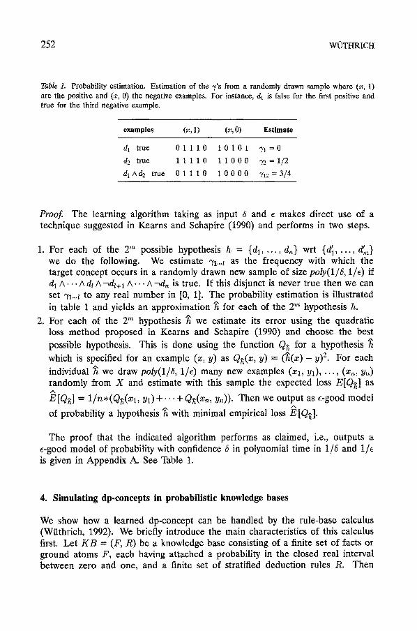
Table i. Probability estimation. Estimation of the 7's from a randomly drawn sample where (x, 1) are the positive and (x, 0) the negative examples. For instance, d 1 is false for the first positive and true for the third negative example.

examples (x, 1) (z, 0) Estimate

d 1 true 0 1 1 1 0 1 0 1 0 1 7 ~ = 0

d 2 true 1 1 1 1 0 1 1 0 0 0 3 '2=1/2

d 1 A d 2 true 0 1 1 1 0 10 0 0 0 712 = 3/4

Proof. The learning algorithm taking as input 5 and e makes direct use of a technique suggested in Kearns and Schapire (1990) and performs in two steps.

1. For each of the 2 '~ possible hypothesis h = {all,. . . , dn} wrt {d~,. . . , d ' } we do the following. We estimate 71-.t as the frequency with which the target concept occurs in a randomly drawn new sample of size poly(1/5, 1/4) if d 1 A . . - A dz A ~dz+l A . . . A-~dn is true. If this disjunct is never true then we can set 71...~ to any real number in [0, 1]. The probability estimation is illustrated in table 1 and yields an approximation ~ for each of the 2 ~ hypothesis h.

2. For each of the 2 '~ hypothesis ~ we estimate its error using the quadratic loss method proposed in Kearns and Schapire (1990) and choose the best possible hypothesis. This is done using the function Q~ for a hypothesis which is specified for an example (z, y) as Q~(x, y) = ( ~ ( x ) - y)2. For each

individual ~ we draw poly(1/5, I/k) many new examples (xl, Yl), . . . , (xn, y,~) randomly from X and estimate with this sample the expected loss E[Q~] as / %

E[Q,~] = 1/n*(Q.~(zl, Y l ) q ' " " 4" Q~(z,~, y,~)). Then we output as e-good model

of probability a hypothesis ~ with minimal empirical loss ~'[Q~].

The proof that the indicated algorithm performs as claimed, i.e., outputs a e-good model of probability with confidence 5 in polynomial time in 1/8 and 1/4 is given in Appendix A. See Table 1.

4. Simulating dp-concepts in probabilistic knowledge bases

We show how a learned dp-concept can be handled by the rule-base calculus (Wfithrich, 1992). We briefly introduce the main characteristics of this calculus first. Let KB = (F, R) be a knowledge base consisting of a finite set of facts or ground atoms F, each having attached a probability in the closed real interval between zero and one, and a finite set of stratified deduction rules R. Then


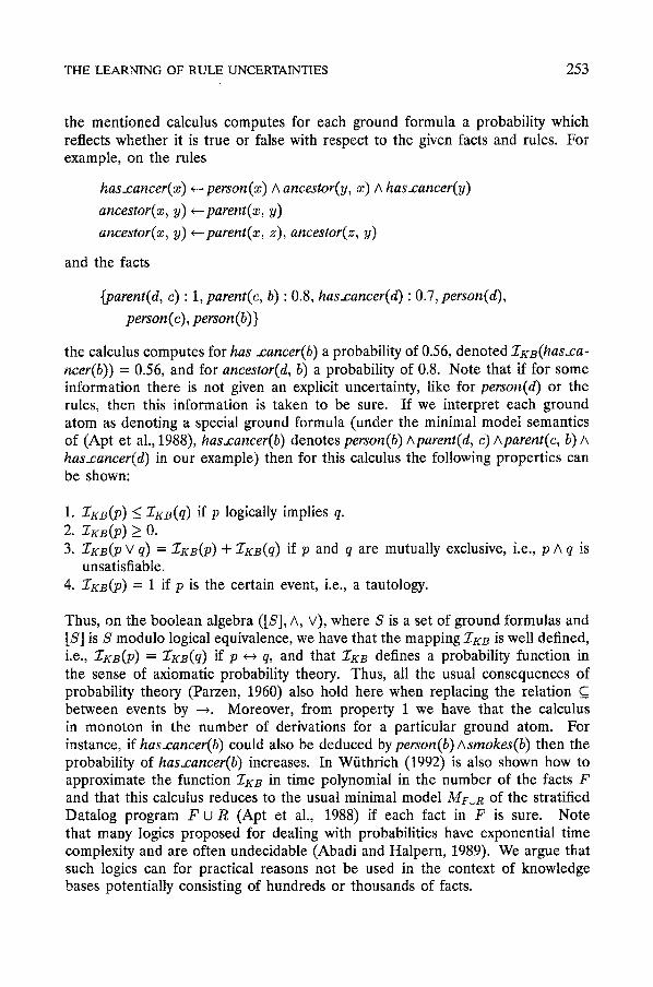
the mentioned calculus computes for each ground formula a probability which reflects whether it is true or false with respect to the given facts and rules. For example, on the rules

has_cancer(x) ~ person(x) A ancestor(y, x) A has_cancer(y) ancestor(x, y) +--parent(x, y) ancestor(x, y) e--parent(x, z), ancestor(z, y)

and the facts

{parent(d, c) : 1, parent(c, b) :0.8, has.cancer(d) :0.7, person(d), person (c), person ( b ) }

the calculus computes for has _cancer(b) a probability of 0.56, denoted ZKn(has-cancer(b)) = 0.56, and for ancestor(d, b) a probability of 0.8. Note that if for some information there is not given an explicit uncertainty, like for person(d) or the rules, then this information is taken to be sure. If we interpret each ground atom as denoting a special ground formula (under the minimal model semantics of (Apt et al., 1988), has_cancer(b) denotes person(b) Aparent(d, e) Aparent(e, b) A has_cancer(d) in our example) then for this calculus the following properties can be shown:

1. IKB(p) <_ :rKB(q) if p logically implies q. 2. ZKB(P) >_ O. 3. ZKB(P V q) = ZKB(P) + ZKB(q) if p and q are mutually exclusive, i.e., p A q is

unsatisfiable. 4. ZKB(P) = 1 if p is the certain event, i.e., a tautology.

Thus, on the boolean algebra ([S], A, V), where S is a set of ground formulas and [S] is S modulo logical equivalence, we have that the mapping ZKB is well defined, i.e., ZKB(P) = ZKB(q) if p ~ q, and that ZKB defines a probability function in the sense of axiomatic probability theory. Thus, all the usual consequences of probability theory (Parzen, 1960) also hold here when replacing the relation c_ between events by --.. Moreover, from property 1 we have that the calculus in monoton in the number of derivations for a particular ground atom. For instance, if has_cancer(b) could also be deduced by person(b)Asmokes(b) then the probability of has_cancer(b) increases. In Wfithrich (1992) is also shown how to approximate the function ZKB in time polynomial in the number of the facts F and that this calculus reduces to the usual minimal model MFon of the stratified Datalog program F u R (Apt et al., 1988) if each fact in F is sure. Note that many logics proposed for dealing with probabilities have exponential time complexity and are often undecidable (Abadi and Halpern, 1989). We argue that such logics can for practical reasons not be used in the context of knowledge bases potentially consisting of hundreds or thousands of facts.

254 WLITHRICH

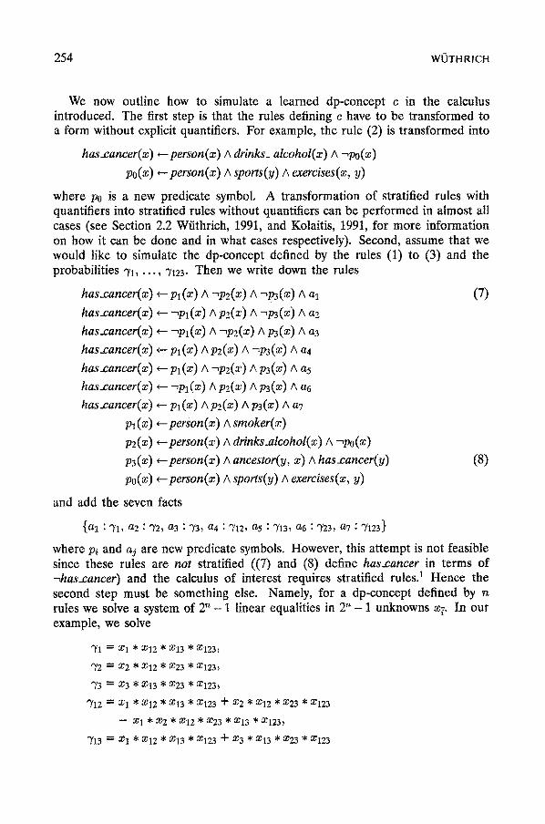
We now outline how to simulate a learned dp-concept c in the calculus introduced. The first step is that the rules defining c have to be transformed to a form without explicit quantifiers. For example, the rule (2) is transformed into

has.cancer(x) ~ person(x) A drinks, alcohol(x) A ~po(x)

po(x) ~person(x) A sports(y) A exercises(x, y)

where p0 is a new predicate symbol. A transformation of stratified rules with quantifiers into stratified rules without quantifiers can be performed in almost all cases (see Section 2.2 Wfithrich, 1991, and Kolaitis, 1991, for more information on how it can be done and in what cases respectively). Second, assume that we would like to simulate the dp-concept defined by the rules (1) to (3) and the probabilities 7a, . . . , '/123. Then we write down the rules

has.cancer(x) ~ p l ( x ) A "~pZ(X) A ~ p 3 ( x ) A a 1 (7)

has.cancer(x) ~ ~pl(x) A p2(x) A -~p3(x) A a2

has.cancer(x) .-- --,pl(X) A ~p2(x) A p3(z) A a3

has.cancer(x) ~ pl(x) A p2(x) A -~p3(x) A a4

has.cancer(x) ~ pl(x) A -~pz(x) A p3(x) A a5

has.cancer(x) +-- ~pl(z) A p2(x) A pa(x) A a6

has.cancer(x) ~ pl(x) A p2(x) A p3(x) A a7

Pa (x) .--person(z) A smoker(x) p2(x) ~ person(x) A drinks.alcohol(x)/x -~po(x) p3(x) .--person(z) A ancestor(y, x) A has_cancer(y) (8)

po(x) .--person(x) A sports(y) A exercises(x, y)

and add the seven facts

{ a l : ' /1, a2 : ' /2, a3 : "/3, a4 : '/12, a5 : "/13, a6 : "/23, a7 : '/123}

where Pi and aj are new predicate symbols. However, this attempt is not feasible since these rules are not stratified ((7) and (8) define has_cancer in terms of -4aas.cancer) and the calculus of interest requires stratified rules. 1 Hence the second step must be something else. Namely, for a dp-concept defined by n rules we solve a system of 2 ~ - 1 linear equalities in 2 ~ - 1 unknowns x z. In our example, we solve

"/1 = Xl * x12 * Z13 * x123~

'/2 ~ z2 * z12 * X23 * x123~

'/3 = Z3 * XI3 * X23 * z123~

'/12 = Xl * z12 * z13 * z123 at- z2 * Z12 * X23 * z123

-- X 1 , z 2 * x 1 2 * z 2 3 * z 1 3 * z 1 2 3 ~

'/13 ~ Z l * X12 * z13 * z123 q- Z3 * z13 * Z23 * ~123

T H E L E A R N I N G O F R U L E U N C E R T A I N T I E S 255

- - x 1 * x 3 * x 1 2 * x 2 3 * x 1 3 * x 1 2 3 ~

"/23 = x 2 * x12 * x23 * x123 + x 3 * x13 * x23 * x123

- - x 2 , x 3 * x 1 2 * x 2 3 * x 1 3 * x 1 2 3 ~

"/123 ---- x l * x12 * x13 * x123 -st- x 2 * x12 * x23 * x123 + x3 * x13 * x23 * x123

- - x l * x 2 * x 1 2 * x 2 3 * x 1 3 * x 1 2 3 - - x 1 * x 3 * x 1 2 * x 2 3 * x 1 3 * x 1 2 3

- - x 2 * x3 * x12 * x23 * x13 * x123 + Xl * x 2 * x3 * x12 * x23 * x13 * x123.

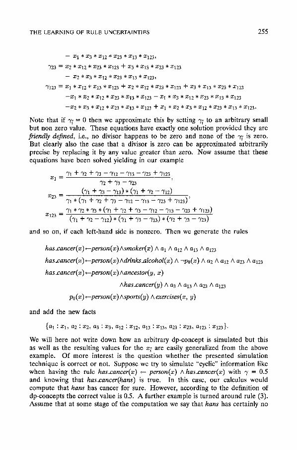
Note that if 97 = 0 then we approximate this by setting 37 to an arbitrary small but non zero value. These equations have exactly one solution provided they are friendly defined, i.e., no divisor happens to be zero and none of the 37 is zero. But clearly also the case that a divisor is zero can be approximated arbitrarily

Now assume that these precise by replacing it by any value greater than zero. equations have been solved yielding in our example

"/1 + "/2 + ")3 - - ")12 - - ")'13 - - ")23 + ")123 X 1 =

72+72 -723 (71 + 73 - - 713) * (71 + 72 - - 712)

X23 = ')1 * ( ')1 + ')2 + ')3 - - ')12 - - ")13 - - ")23 + ')123) '

")/1 * "/2 * '~3 * ( ')1 + ')2 + ")3 - - ')12 - - ")13 - - ")'23 + ')123)

X123 = (')/1 + "/2 - - ' )12) * (71 + ')3 - - '713) * ( 72 + ')3 - - ' )23)

and so on, if each left-hand side is nonzero. Then we generate the rules

has_cancer(x) ~person(x)Asmoker(x) A al A a12 A a13 A a123

has_cancer(x)*--person(x) Adrinks_alcohol(x) A -,po(x) A a2 A a12 A a23 A a123

has_cancer( z ) ~ person ( z ) A ancestor( y , x)

Ahas_cancer(y) A a3 A a13 A a23 A a123

po(x) ~person(x) Asports(y) A exercises(x, y)

and add the new facts

{ a l : Xl~ a2 : x2~ a3 : x 3 , a12 : x12~ a13 : x13~ a23 : x23 , a123 : x123} .

We will here not write down how an arbitrary dp-concept is simulated but this as well as the resulting values for the x i are easily generalized from the above example. Of more interest is the question whether the presented simulation technique is correct or not. Suppose we try to simulate "cyclic" information like when having the rule has_cancer(x) +-- person(x) A has_cancer(x) with 7 = 0.5 and knowing that has_cancer(hans) is true. In this case, our calculus would compute that hans has cancer for sure. However, according to the definition of dp-concepts the correct value is 0.5. A further example is turned around rule (3). Assume that at some stage of the computation we say that hans has certainly no

256 WI]THRICH

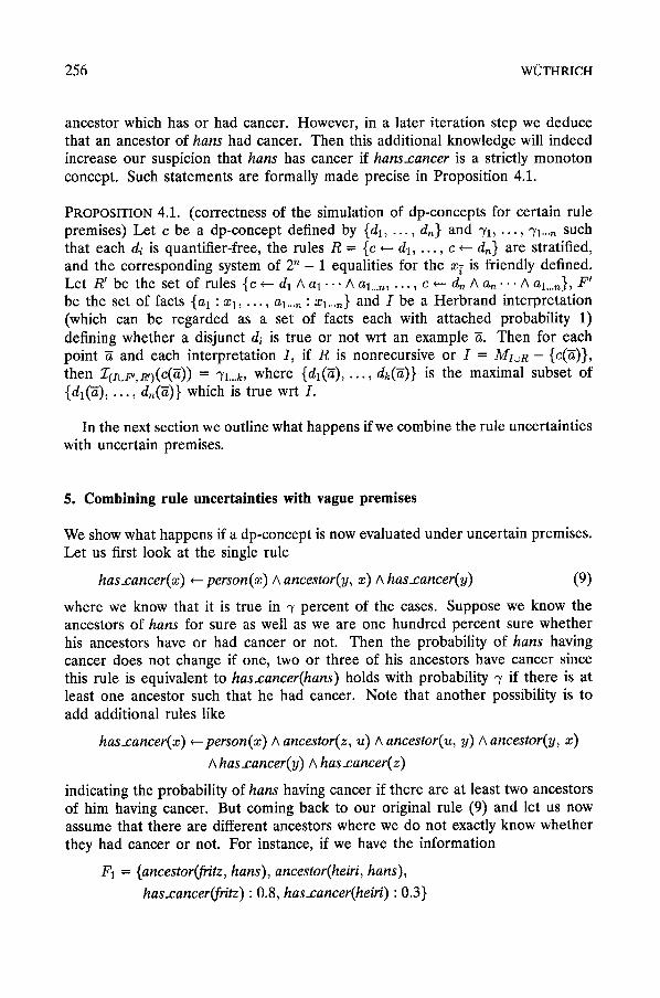
ancestor which has or had cancer. However, in a later iteration step we deduce that an ancestor of hans had cancer. Then this additional knowledge will indeed increase our suspicion that hans has cancer if hans_cancer is a strictly monoton concept. Such statements are formally made precise in Proposition 4.1.

PROPOSITION 4.1. (correctness of the simulation of dp-concepts for certain rule premises) Let c be a dp-concept defined by {dl, . . . , d,~} and 7a, . - . , "Yl...,~ such that each di is quantifier-free, the rules R = {e ~ dl, . . . , c ~ dn} are stratified, and the corresponding system of 2 n - 1 equalities for the x 7 is friendly defined. Let R' be the set of rules {c +-- da A al . . . /x al ..... . . . , c *-- dn A a n " ' A aL.n}, F ' be the set of facts {al : xl , . . . , al .... : Xl...n} and I be a Herbrand interpretation (which can be regarded as a set of facts each with attached probability 1) defining whether a disjunct di is true or not wrt an example ~. Then for each point g and each interpretation 1, if R is nonrecursive or I = Miua - {c(g)}, then Z(zuF,,n,l(e('~)) = " ) ' l . . . k , where { d l ( a ) , . . . , dk(g)} is the maximal subset of {dl(~), . . . , dn(g)} which is true wrt I.

In the next section we outline what happens if we combine the rule uncertainties with uncertain premises.

5. Combining rule uncertainties with vague premises

We show what happens if a dp-concept is now evaluated under uncertain premises. Let us first look at the single rule

has_cancer(x) ~ person(x) A ancestor(y, x) A has_cancer(y) (9)

where we know that it is true in ~' percent of the cases. Suppose we know the ancestors of hans for sure as well as we are one hundred percent sure whether his ancestors have or had cancer or not. Then the probability of hans having cancer does not change if one, two or three of his ancestors have cancer since this rule is equivalent to has_cancer(hans) holds with probability 7 if there is at least one ancestor such that he had cancer. Note that another possibility is to add additional rules like

has.cancer(x) e--person(x) A ancestor(z, u) A ancestor(u, y) A ancestor(y, x) h has_cancer(y) h has_cancer(z)

indicating the probability of hans having cancer if there are at least two ancestors of him having cancer. But coming back to our original rule (9) and let us now assume that there are different ancestors where we do not exactly know whether they had cancer or not. For instance, if we have the information

F1 = {ancestor(fritz, hans), ancestor(heiri, hans), has_cancer(fritz) : 0.8, has.cancer(heiri) : 0.3}


then the probability of hans having cancer deduced by means of the rule (9) should be greater than when simply having either of the following information

F2 = {ancestor(fritz, hans), has_cancer(fritz) : 0.8},

F3 = {ancestor(heiri, hans), has.cancer(heiri) : 0.2),

F4 = {ancestor(fritz, hans), ancestor( heiri, hans), has_cancer(fritz) : 0.8},

F5 = {ancestor( heiri, hans), ancestor(fritz, hans), has_cancer( heiri) : 0.2}.

Note that we could also express the ancestor relation by means of the two standard rules using the parent information and everything would work fine. We use our concepts introduced, with a rule probability -~ = 0.1 for (9) and get

0.08 = Z(F2, {(9)})(has_cancer(hans) = Z(F,, ((9)})(has_cancer(hans)), 0.02 = Z(F3, ((9)})(has_cancer(hans)) = Z(Fs, {(9)})(has_cancer(hans)),

0.084 = Z(F1, {(9)})(has_cancer(hans)).

Now let us take an example with the two rules (9) and

has.cancer(z) ~ person(z) A smoker(z) (10)

with rule uncertainties ~'1, 3'2 and 712 for rule (9), (10), and both respectively. Assume that there is some vagueness in the ancestor and smoking information. Then our method computes on the set of facts

F = {ancestor(fritz, hans) : 0.9, has_cancer(fritz) : 0.8,

ancestor(heM, hans), has_cancer(heiri) : 0.2, smoker(hans) : 0.9}

the probability Z(F,((9),Oo)} }(has-cancer (hans)) abbreviated by Pr[has_cancer (hans)] (we will use this abbreviation also below when it is clear to which facts and rules we refer) to be

Pr[p(hans) A (a(fritz, hans) A h_c(fritz)Va(heiri, hans) A h_c(heiri)) A-~(p(hans) A s(hans))] �9 3'1

+ Pr[p(hans) A s(hans) A -~(p(hans) A (a(fritz, han s) A h_c(fr/tz) va(heiri, hans) A h_c(heiri))] �9 3'2

+ Pr[p(hans) A s(hans) A (a(fritz, hans) A h_c(fritz) Va(heiri, hans) h h_c(heiri))] �9 712

= ( 0 . 9 �9 0 . 8 + 0 . 2 - 0 . 9 �9 0 . 8 �9 0 . 2 ) �9 (1 - 0 . 9 ) �9 ")'1

+ 0.9 �9 (1 - (0.9 �9 0.8 + 0.2 - 0.9 �9 0.8 �9 0.2)) �9 72 + 0.9 �9 (0.9 �9 0.8 + 0.2 - 0.9 �9 0.8 �9 0.2) �9 ")'12

= 0.0776 �9 ~'1 + 0.2016 �9 "Y2 + 0.6984 �9 "r12

where we abbreviated person, ancestor, smoker and has_cancer by p, a, s and h_c respectively. Proposition 5.1 gives the precise information on what actually happens in the nonrecursive case and assures the correctness of the combination of rule uncertainties with vague premises under the assumption that the rule

258 WOTHRICH

uncertainties are independent from the premise uncertainties. Note that we could not find an intuitively appealing correctness criterion for recursive dp-concepts since the definition of dp-concepts itself is inherently nonrecursive.

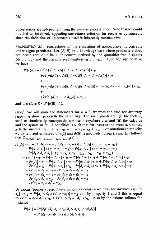
PROPOSITION 5.1. (correctness of the simulation of nonrecursive dp-concepts under vague premises). Let (F, R) be a knowledge base where predicate c does not occur and let c be a dp-concept defined by the quantifier-free disjuncts {d l , . . . , d~} and the friendly real numbers 71, . . . ,%..~. Then for any point ~, we have

Pr[c(E)] = Pr[dl(E) A -~d2(E) A . . . A ~d,~(E)] �9 71

+er[-,d~('a) ^ d2(n) ^ - ,d3(n) A . . . ^ - , d , ( ~ ) ] �9 72 + . . .

+Pr[-~dl('~) ^ d2(~) ^ -~d3(n) ^ d4(~) A - ,ds (n ) ^ . . . ^ - ,d~(~)] �9 724 + . . .

+Pr[dl('a) ^ . . . ^ d , ( ~ ) ] �9 7~...,

and therefore 0 _< Pr[c(-d)] <_ 1.

Proof. We will show the statements for n = 3, whereas the case for arbitrary large n is shown in exactly the same way. The main points are: (i) the facts ai used to simulate dp-concepts do not occur anywhere else and (ii) the calculus and the system of 2 '~ - 1 equalities is such that for instance the event as A aj A ak gets the uncertainty q'i + 7j + 7k - 7ij - 7i~ - 7jk + 70k- For notational simplicity we write c and di instead of c(~) and di(~) respectively. From (i) and (ii) follows that Z(F, nu{~-dl~r..a~ ......... c,_d.,~...a~.M)(c) is

er[dl] * 71 + er[d2] �9 3'2 + er[d3] * 73 - er[dl A d2] * (71 q" 72 - - 712)

- Pr[dl ^ d3] �9 (71 + 73 - 7~3) - Pr[d2 ^ d31 * (72 + 73 - 723) +Pr[dl h d2 A d3] * (71 + '72 + 73 - 712 - - 713 - - 723 + 7 t 2 3 )

= Pr[d~] �9 7~ - Pr[dl ^ dE] * 71 - Pr[dl ^ d3] * 71 + Pr[dl ^ dz A d3] * 71 + Pr[d2] * 72 - er[dl A d2] * 72 - Pr[d2 A d3] * 72 + Pr[dl A d,2 A d3] * 72 + Pr[d3] * 73 - Pr[dl A d31 * 73 - Pr[d2 A d3] * 73 + Pr[dl A de A d31 * 73 + Pr[dl ^ dE] * 7~2 - Pr[d~ ^ d2 ^ d3] * 7~2 + Pr[d~ ^ 43] * 713 - Pr[d~ ^ d2 ^ d3] * 7~3 + Pr[dz ^ d3] * 713 - Pr[dl ^ d2 ^ d3] * 723 + Pr[d~ ^ d2 ^ d3] * 7123.

By axiom (property respectively for our calculus) 4 we have for instance Pr[dl A da] * "Yla -- Pr[dl h da A (d3 V ~d3)] * 3'1z and by property 1 and 3 this is equal to Pr[dl A dz h d3] * 71z + Pr[dl A d~ A -~d3] * 712. Also by the axioms follows for instance

Pr[dl] = Pr[dl(-~d2-~d3 V da~d3 V d2d3 v --,dzd3)]

= Pr[dl-,d2~d3] + Pr[dl(d2 V d3)]


= Pr[dl~d2~d3] + Pr[dld2] + Pr[dld3]-Pr[dld2d3].

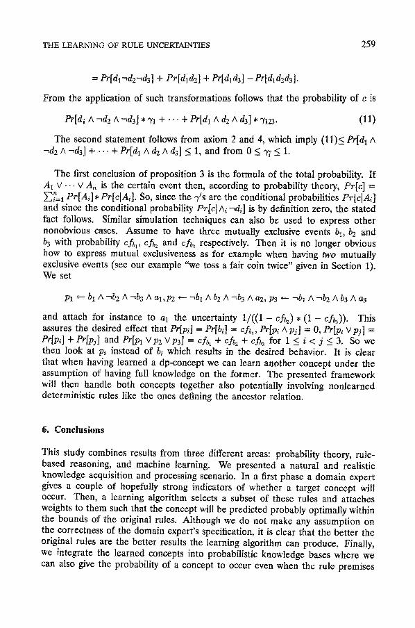
From the application of such transformations follows that the probability of c is

Pr[dl A -~d2 A "~d3] * ~/1 + ' " + Pr[dl A d2 A dx] * "/123. (11)

The second statement follows from axiom 2 and 4, which imply (11)_< Pr[dl/x -,d2 A --,d3] + ... + Pr[dl A d2 A d3] < 1, and from 0 < 37 -< 1.

The first conclusion of proposition 3 is the formula of the total probability. If As v - . . V An is the certain event then, according to probability theory, Pr[c] = ~i~=1 Pr[A d * Pr[clAi]. So, since the ,/s are the conditional probabilities Pr[ctAi ] and since the conditional probability Pr[c[ Ai-,d~] is by definition zero, the stated fact follows. Similar simulation techniques can also be used to express other nonobvious cases. Assume to have three mutually exclusive events bl, b2 and ba with probability cfbl, cf~ and cfb3 respectively. Then it is no longer obvious how to express mutual exclusiveness as for example when having two mutually exclusive events (see our example "we toss a fair coin twice" given in Section 1). We set

Pl r 51 A ~b2 A ",b 3 A al,P2 +.- "rib 1 A b2 A ~b3 A a2, t93 ~- ~bl A ~b2 A b3 A a3

and attach for instance to al the uncertainty 1 / ( ( 1 - c f ~ ) , ( 1 - cfb3)). This assures the desired effect that Pr[pi] = Pr[bl] = cf~l, Pr[pi hp~] = 0, Pr~i Vp3] = Pr[p d + Pr[pj] and Pr[pl V P2 V P3] = cfb~ + cfh + cfb3 for 1 < i < j _< 3. So we then look at pl instead of bi which results in the desired behavior. It is clear that when having learned a dp-concept we can learn another concept under the assumption of having full knowledge on the former. The presented framework will then handle both concepts together also potentially involving nonlearned deterministic rules like the ones defining the ancestor relation.

6. Conclusions

This study combines results from three different areas: probability theory, rule- based reasoning, and machine learning. We presented a natural and realistic knowledge acquisition and processing scenario. In a first phase a domain expert gives a couple of hopefully strong indicators of whether a target concept will occur. Then, a learning algorithm selects a subset of these rules and attaches weights to them such that the concept will be predicted probably optimally within the bounds of the original rules. Although we do not make any assumption on the correctness of the domain expert's specification, it is clear that the better the original rules are the better results the learning algorithm can produce. Finally, we integrate the learned concepts into probabilistic knowledge bases where we can also give the probability of a concept to occur even when the rule premises

260 WI~ITHRICH

are vague. Moreover, different learned concepts and non-learned deterministic rules can be added together yielding a large uniform knowledge base.

The presented knowledge acquisition scenario merges expert knowledge and automatic inference methods. Friedland and Kedes (1985) propose such a combination in a less specific form: 'N basic lesson learned is that relatively simple reasoning or inference methods could be most effectively applied to problem solving when they were accompanied by a large amount of diverse expert knowledge". But also to rely on an extension of Valiants' learning model seems quite natural. Valients learning model was used to give the first provably good approximation algorithm for determining the shortest common superstring (DNA sequence) from a set of strings (set of fragments of the DNA sequence) (Li, 1990). Hence, this model can be used to mathematically determine whether a functionality is encoded in a specific DNA structure. This is because the latter problem reduces to the question whether a given gene (string over the four nucleotides) is part of the DNA (is a substring of the DNA string) visible only through samples of fragments obtained by cutting it up.

We believe that a prerequisite for a successful real world application of uncertain information in knowledge bases is to have available a "good" uncertainty calculus as well as "good" uncertainties themselves. We hope we have satisfied both prerequisites.

Acknowledgments

I would like to thank G. Comyn and ECRC for the support when doing this work and V. Valkovsky for the encouraging and fruitful discussions.

Appendix A: Correctness of the Learning Algorithm

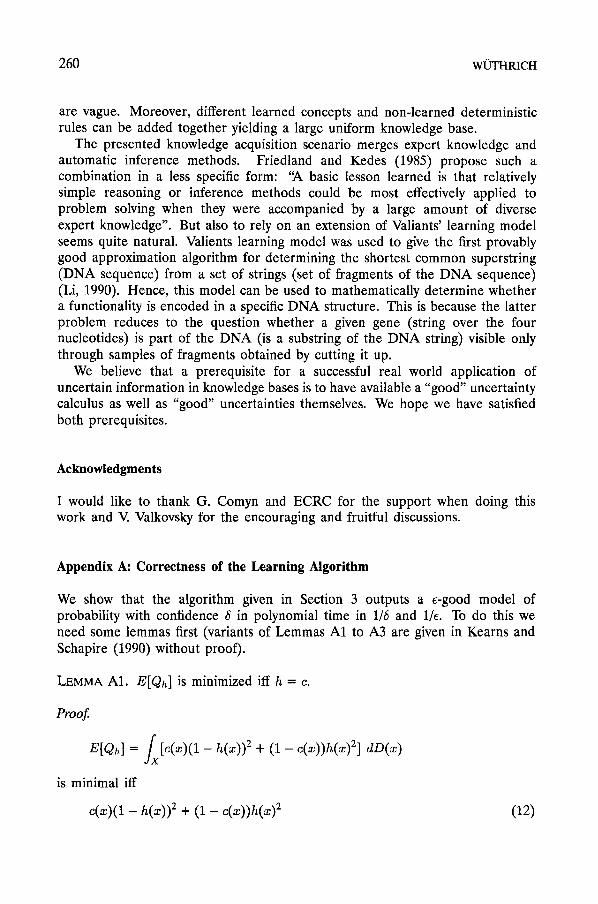
We show that the algorithm given in Section 3 outputs a e-good model of probability with confidence 6 in polynomial time in 1/6 and 1/e. To do this we need some lemmas first (variants of Lemmas A1 to A3 are given in Kearns and Schapire (1990) without proof).

LEMMA A1. E[Qh] is minimized iff h = c.

Proof.

E[Qh] = fx[C(X)(1 - h(x)) 2 + (1 - c(x))h(x) 2] dD(x)

is minimal iff

c(z)(1 - h(x)) 2 + (1 - c(x))h(x) 2 (12)

T H E L E A R N I N G OF R U L E UNC E R T AINT IE S 261

is minimal for each x. But (12) is minimal for some x iff - 2 c ( x ) ( 1 - h(x)) + 2 ( 1 - c(x))h(x) = 0. Thus, (12) is minimal for some x iff h(x) = c(x), hence E[Qh] is minimal h = c.

We deno te by Pr[A(x)] the probabil i ty of event A(x) which depends on x E X if x is drawn according to the distr ibution D.

LEMMA A2.

E[Qh] -- E[Qc] < e3---->Pr[lh(x) - c(x)[ < e] >__ 1 - e.

Proof Assume Pr[lh(x ) - c(x)[ < e I < 1 - e or equivalent ly Pr[lh(x ) - c(x)[ __ e I >__ e. T h e n we get f x (h(x) - c(x))2dD(x) > e 3. But now, as shown on page

386 in Kearns and Schapire (1990), E[Qh]- E[Qc] = f x ( h ( x ) - c(x))2dD(x), thus E [ Q h ] - E[Qc] _> e 3, a contradict ion.

L E M M A A 3 .

Pr[Ih(x ) - ~(x)[ < 7"1] _.~ 1 - T2~[E[Qh] -- E[Q~][ < T 1 * 11 + T 2.

Proof. From the premise we have

[E[Qh] - E [ % l l

fx[C(1 - h) 2 + (1 - c)h 2 - c(1 - h 4- 7-1) 2 - (1 - c)(h 4- T1)2]dD(x) < +7 - 2.

By simplification we get for the lat ter t e rm r1(+2c 4- 4oh + or1 4- 2h + 2r l ) + r2, which is not m ore than rl * 11 + r2.

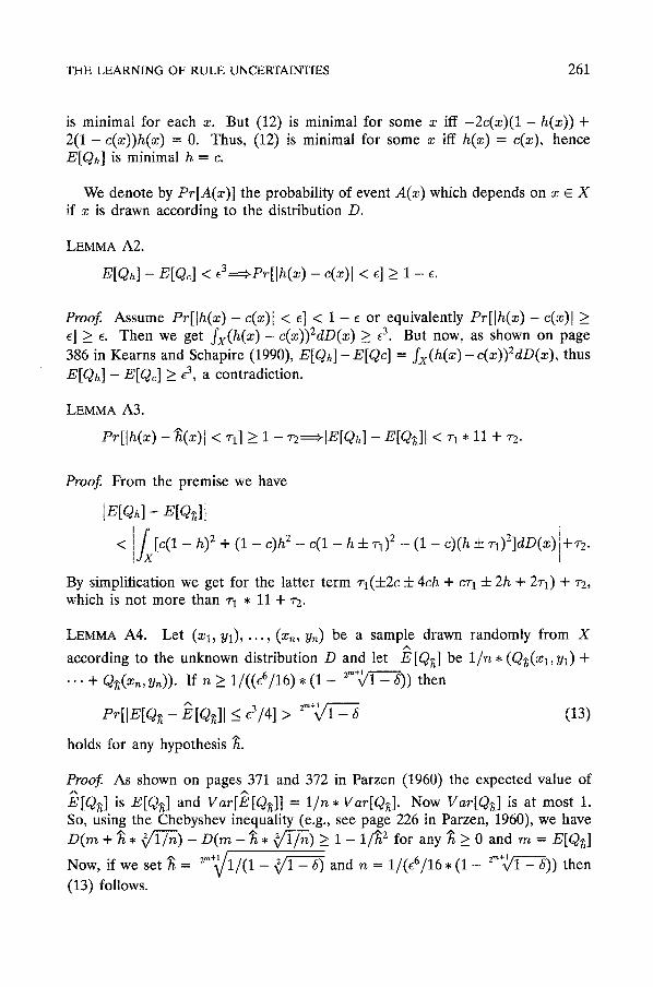
LEMMA A4. Le t (xl , Yl), . . . , (zn, Yn) be a sample drawn randomly f rom X A

according to the unknown distr ibution D and let E [Q~] be 1/n * (Q~(xt, yl) +

. . . + Q~(xn, y~)). If n _> 1/( (e6/16) * (1 - 2~,§ 5)) then

_ 2m§ Pr[IE[Q~ - E[Q~]I < e3/4] > - 5 (13)

holds for any hypothesis ~.

Proof As shown on pages 371 and 372 in Parzen (1960) the expec ted value of

E[Q~] is E[Q~] and Var[E[Q,~]] = l / n * Var[Q.~]. Now Var[Q~] is at mos t 1. So, using the Chebyshev inequali ty (e.g., see page 226 in Parzen, 1960), we have

D ( m + "~ �9 ~/ i -~) - D ( m - ~ �9 ~/]'7-~) > 1 - 1 /~ 2 for any ~ > 0 and m = E[Q~]

Now, if we set ~ = 2m+~l/(1 - ~ " i - 6) and n = 1 / ( e 6 / 1 6 . ( 1 - 2m+~ff- 5)) t hen

(13) follows.

262 WOTHRICH

E[Oi,]

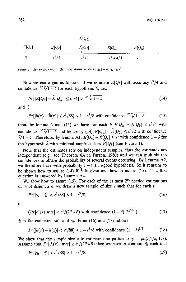
E[Oc] E[Q~] E[Q~] E[Qi,] E[Qh ] I I I I I

0 (3/4 E3/2 E 3 * 3/4 f3

Figure I. The worst case of the estimations yields E [ Qh] - E[Qc] < e 3.

Now we can argue as follows. If we estimate E[Q,~] with accuracy 43/4 and

confidence 2"~1 - 6 for each hypothesis ~, i.e.,

- _ 2 ~ ' § Pr[IE[Q,~] E[Q~]I < e3/4] > -- 5 (14)

and if

Pr[Ih(x ) - ~(x)[ < e3/88] > 1 - ,3/8 with confidence 2"§ - 5 (15)

then, by lemma 3 and (15) we have for each h E [ Q h ] - E[Q.~] < 43/4 with

confidence 2"§ and hence by (14) E[Qh]- E[Q~] < ,3/2 with confidence 2~/]-_ 6. Therefore, by lemma A1, E[Qh] - E[Qc] < 43 with confidence 1 - 6 for

A

the hypothesis ~ with minimal empirical loss E[Q,~] (see Figure 1).

Note that the estimates rely on independent samples, thus the estimates are independent (e.g., see Theorem 6A in Parzen, 1960) and we can multiply the confidences to obtain the probability of several events occurring. By Lemma A2, we therefore have with probability 1 - 6 an 4-good hypothesis. So it remains to be shown how to assure (14) if ~ is given and how to assure (15). The first question is answered by Lemma A4.

We show how to assure (15). For each of the at most 2 m needed estimations of 74 of disjuncts d~ we draw a new sample of size s such that for each i:

Pr[l'~ - ~1 < e3/88] > 1 - e3/8, (16)

o r

(Pr[d4(z),truel < ,3/(2m* 8) with confidence (1 - 6 ) 1/(2m+1)) (17)

~4 is the estimated value of 7~. From (16) and (17) follows

er[lh(z ) - ~(z)l < ,3/88] > 1 - 43/8 with confidence (1 - 6) 1/2 (18)

We show that the sample size s to estimate one particular 0'4 is poly(1/6, 1/,). Assume that Pr[di(z), true] > 43/(2m* 8) then we have to compute @4 such that

Pr[174 - ~1 < '3/88] > 1 - 43/8. (19)


To do this we need poly(1/E) many examples where di is true by a standard Chernoff bound analysis (e.g., see page 18 in Kearns, 1990, and take there into account that we set r := /3/2 and p := /~ to obtain correct results if 1/p < 1/r The estimation is done by letting ~i be the frequency with whicli the concept occurs. To get with a confidence of (1 - 6 ) 1/2m§ (1/6, l /e) many examples where di is true, we also need only poly(1/6, l /e) many examples since Pr[di(x) true] >. e3/(2m* 8) (the statement that we need again only poly I/E, l /e) many examples is verified below). If we do not get enough examples then we assume Pr[di(x) true] < E3/(2 m * 8) to hold. This assumption is true with confidence ( 1 - 6) 1/2~*~. This shows how to assure (16),(17), thus (18) and hence (15).

Finally, we complete the arguments that the given learning algorithm runs in time polynomial in 1/6 and t/e. First we show that the number n of needed examples in Lemma A4 is poly(l/6, t / @ So we have to show that 1/((e6/16), ( 1 - 2m+~/1- 6)) is polynomial in 1/6 and 1/e. This is assured if 1 / ( 1 - 2r~§ __< (1/6) x for some fixed x. So we have to show 1 - ( 1 - 6 ) 1/2"~§ > 6 ~ from which follows 6 / 2 m+l > 6 z by the fact that ( 1 -6 ) t/2m+l _< 1 - 6 / 2 m+l. But 6 / 2 m+l :> 6 z is true for x = 2 if 0 < 6 < 1/2 "~+1. And the case 6 > 1/2 m+l is not interesting since then we can set 6 = 1/2 m+l. Second, we have to show that in order to draw poly(t/~, l /e) many successful examples (examples x where d4(x) is true) with confidence ( 1 - 6) 1/2=.1, we again need only poly(1/delta, l /e) many trials if the probability of success is at least e3/(2 m �9 8). From the proposition given in Valiant (1984) immediately follows that we therefore have to show that h -1 = min(e3/(2m, 8), 1 - ( 1 - 6 ) V2~§ is polynomial in 1/e and 1/& If e3/(2 m,8) _< 1 - ( 1 - 6) 1/2m§ we are done. Otherwise, this proposition implies that we have to show L(h,poly(1/6, l /e)) _< 2 �9 (1 - (1 - 6)1/2~+~) -1 �9 (poly(1/6, l /e) + ln(1 - (1 - 6)1/2"§ So we have to show (1 - (1 -/6)1/2~§ -1 _< (1/6) ~' for

some fixed z. Using ( 1 - 6) 1/2~§ <_ 1 - 6/2 "~+1, it remains to be shown that ~/2 ~+1 >_ ~ for some fixed x. But ~/2 ~+1 _> 62 holds if 0 < 6 < 1/2 m+l. And the case 6 > 1/2 ~+1 is not interesting since then we can set 6 = 1/2 ~+1. This completes the proof of the correctness of the learning algorithm.

Notes

1. There is an even deeper problem with this approach. If the calculus is used in such a "false" way, assuming that local stratification is sufficient, then monotonic @-concepts can become nonmonotonic.

264 WOTHRICH

References

Abadi, M. & Halpern, J.Y. (1989). Decidability and Expressiveness for First-Order Logics of Proba- bility, Proc. 30st IEEE Syrup. on Foundations of Computer Science, pp. 148-153. Brass, S. (1992). Defaults in Deduktiven Datenbanken. Ph.D. thesis, University of Hannover, Germany. Apt, K.R., Blair, H.A., & Walker A. (1988). Towards a Theory of Declarative Knowledge. In J. Minker (Ed.), Foundations of Deductive Databases and Logic Programming. Morgan Kaufmann: Los Altos, CA. Friedland, P. & Kedes, L.H. (1985). Discovering the Secrets of DNA, Communications of the ACM, 28(11), 1164-1186. Halpern, J.Y. & Rabin, M.O. (1983). A Logic to Reason about Likelihood, Proc. Annual ACM Symp. on the Theory of Computing, pp. 310--319. Kearns, M.J. (1990). The Computational Complexity of Machine Learning, MIT Press. Kearns, M.J. & Schapire, R.E. (1990). Efficient Distribution-Free Learning of Probabilistic Concepts, Proc. 31st IEEE Syrup. on Foundations of Computer Science, pp. 382-391. Kolaitis, EG. (1991). The Experessive Power of Stratified Logic Programs, Information and Compu- tation, 90(1), 50-66. Li, M. (1990). Towards a DNA Sequencing Theory, Proc. 31st Syrup. on Foundations of Computer Science, pp. 125-134. Muggleton, S. (1990). Inductive Logic Programming, New Generation Computing, 8, 195-318. Natarajan, B.K. (1991). Machine Learning. A TheoreticaIApproach, Morgan Kaufmann: San Mateo, CA. Parzen, E. (1960). Modern Probability Theory and its Applications, Wiley : New York. Pitt, L. & Valiant, L.G. (1988). Computational Limitations on Learning from Examples, Journal of the ACM, 35(4) 965-984. Rich, E. (1983). Default Reasoning as Likelihood Reasoning, Proc. National Conf. on Artif. lnteU. (AAAI), pp. 348-351. Schiiuble, E & Wiithrich, B. (1993). On the Expressive Power of Query Languages, ACM Transactions on Information Systems. (Forthcoming). Valiant, L.G. (1984). A Theory of the Learnable, Communications of the ACM, 27(11), 1134-1142. Valiant, L.G. (1985). Learning Disjunctions of Conjunctions, Proc. Int. Joint Conf. on Artif. Intell. (IJCAI), pp. 560-566. Wiithrich, B. (1991). Large Deductive Databases with Constraints, Ph.D. thesis, Swiss Federal Institute of Technology (ETH) Zurich, Switzerland. Wiithrich, B. (1992). Probablistic Knowledge Bases, submitted. Wiithrich, B. (1993). Learning Probabilistic Rules, Tech. Report, No. 93-3, European Computer Industry Research Center (ECRC).

on the learning of rule uncertainties and their integration into probabilistic knowledge bases

Documents