on the interaction between patent screening and its
TRANSCRIPT

On the Interaction between Patent Screening and itsEnforcement∗
Gerard LlobetCEMFI and CEPR
Alvaro ParraUBC Sauder
Javier SuarezCEMFI and CEPR
January 21, 2021
Abstract
This paper explores the interplay between patent screening and patent enforcement.Costly enforcement involves type I and type II errors. When the patent officetakes the rates at which such errors occur as given, granting some invalid patentsis socially optimal even in the absence of screening costs because it encouragesinnovation. When the influence on courts’ enforcement effort is considered, thesesame forces imply that screening and enforcement are complementary. This meansthat, contrary to common wisdom, better screening induces better enforcement butalso that an increase in enforcement costs could be optimally accommodated withless rather than more ex-ante screening.
JEL Codes: L26, O31, O34.Keywords: Intellectual Property, Innovation, Imitation, Patent Screening, PatentEnforcement, Industry Dynamics.
∗This work is based on a previous paper entitled “Entrepreneurship Innovation, Patent Protec-tion, and Industry Dynamics.” Financial support from the European Commission (grant CIT5-CT-2006-028942) and the Spanish Ministry of Science and Innovation through the ECO2008-00801, theConsolider-Ingenio 2010 Project “Consolidating Economics” and the Regional Government of Madridthrough grant S2015/HUM-3491 is gratefully acknowledged. Address for correspondence: Gerard Llobet,CEMFI, Casado del Alisal 5, 28014 Madrid, Spain. Tel: +34-914290551. Fax: +34-914291056. Email:[email protected].
1 Introduction
In recent decades, we have witnessed a surge in patenting activity. The large number of
applications has put a strain on patent offices everywhere. There is a concern that this
process might have led to a proliferation of likely invalid patents that could hinder future
technological progress, particularly in areas where innovation is cumulative. Between 75%
and 97% of the applications reviewed by the US Patent and Trademark Office (USPTO)
end up in a patent being granted (Lemley and Sampat, 2008). To address this issue, many
authors advocate to increase the resources of patent offices (c.f., Farrell and Merges,
2004).1 Others, however, argue that the high approval rates are the consequence of
rational ignorance (Lemley, 2001): Since only a tiny fraction of patents is ever litigated,2
performing in-depth ex-post screening through litigation, rather than carefully analyzing
ex-ante whether each patent is valid and relevant, can be more cost effective.3
In this article, we study the interplay between ex-ante screening by the patent office
and ex-post enforcement by courts, and their impact on innovation and welfare. We
show that when courts are imperfect—i.e., there is a positive chance to make an incorrect
ruling—and these mistakes are regarded independent from the patent office’s behavior,
some rational ignorance by the patent office is socially optimal even in the absence of
screening costs. That is, even when ex-ante screening could be perfect at no cost, it could
be optimal to allow a percentage of invalid patents. On the other hand, when courts’
mistakes depend on judges’ endogenous effort (as in Daughety and Reinganum (2000))
ex-ante screening and ex-post enforcement are complementary. That is, an increase in
screening by the patent office facilitates court decisions, leading to better rulings.
To study the interaction between patent screening and enforcement, we propose a
tractable industry-dynamics model with sequential innovation and endogenous entry. The
1This view has been adopted in the Leahy-Smith America Invents Act of 2011 that increases fundingand provides new screening mechanisms to better discern the quality of patent applications.
2 Lemley (2001) estimates that 2% of patents are litigated and only about 0.2% of patents reach acourtroom.
3Frakes and Wasserman (2019) challenge the results of this cost-benefit analysis.
2

industry is made up of a continuum of business niches, each of which can be thought of
as the market for a distinct product. Successful developers of improved versions of each
product contribute to welfare and appropriate temporary monopoly profits as in a stan-
dard quality ladder model with limit pricing (Grossman and Helpman, 1991; Aghion and
Howitt, 1992). These temporary monopolies are based on intellectual property (IP) pro-
tection and are threatened by the endogenous arrival of two kinds of entrants: developers
of better versions of the product (that we denote as genuine innovators) and entrants
that contribute minor improvements with little social value (that we denote as obvious
innovators).4
In every period, entrants observe market conditions and invest in R&D until the quasi-
rents from entry are dissipated. Entrants face uncertainty on whether their product will
infringe existing IP rights and, as a result, they suffer from the “tragedy of anticommons”
(Heller and Eisenberg, 1998). This assumption is consistent with Lemley (2008) who
argues that, due to the large number of overlapping rights, firms decide to innovate first,
ignoring related patents, and deal later with the lawsuits that ensue from existent patent
holders. This strategy is also supported by the large proportion of patents brought to
court that end up invalidated (Allison and Lemley, 1998).
Upon entry, firms may randomly produce a genuine or an obvious innovation. En-
trants apply first for a patent and only learn the quality of their innovation through the
commercialization of their products. Patent applications are presumed valid, as patent
examiners have to find prior art and articulate an appropriate basis for rejection. This
means that genuine innovators always receive a patent but the success of an obvious in-
novator depends negatively on the amount of resources that the patent office devotes to
screening—the screening rate. This assumption is consistent with the findings in Frakes
and Wasserman (2017), which shows that lack of resources by patent examiners (e.g.,
4We assume that obvious innovations do not fulfill the novelty requirements for patentability norrepresent a sufficient innovative step to place them outside the breadth of existing patents. Genuineinnovations satisfy both.
3

tighter time constraints) results in a bias towards an increase in the approval rate.5
After a patent has been obtained, an entrant may randomly reach a competitive niche
or one monopolized by an incumbent. A genuine innovator monopolizes a competitive
niche, while an obvious innovator keeps the niche competitive, as it introduces a product
of similar quality to those in the market. If the entrant lands in a monopolized niche, the
incumbent goes to court to preserve its rents by claiming that the entrant infringes on its
patent. If the court rules in favor of the entrant both firms compete in the same niche,
driving the incumbent’s profits to zero, whereas the entrant makes profits according to
its quality. If the court determines that the entrant has infringed the incumbent’s patent,
the innovation goes to waste.
The strength of patent protection is endogenous. Each case that arrives to court
is decided by a different judge. Judges can err in their rulings. Consequently, patent
protection is probabilistic, reflecting the uncertainty on the enforcement of existing patents
(c.f., Lemley and Shapiro, 2005; Farrell and Shapiro, 2008).6 For each case, a judge decides
how much costly effort to devote to analyzing the evidence. Although both the patent
office and judges choose their effort with the objective to maximize social welfare, their
decisions are taken at different stages of the entry process. Whereas the patent office
oversees every patent application, courts only evaluate the validity of a patent conditional
on an entrant having reached a monopolized niche. As we explain below, this asymmetry
creates a dynamic (in)consistency problem within the patent system.
A judge’s objective function can be written as a weighted average of the welfare costs
of committing type I and type II errors. A type I error arises when a judge rules against an
entrant with a genuine innovation, depriving society from the benefit of that improvement.
A type II error arises when an obvious innovator is allowed to compete with the existing
5The authors also show that the bias towards patenting created by shortening the allocated time forthe reviewing process is more prominent in industries where technologies are complex and innovation issequential, as in the framework discussed in this paper. See also Lei and Wright (2017).
6Other work in which courts make probabilistic rulings include Spier (1994), Daughety and Reinganum(1995), and Landeo et al. (2007). By adopting this probabilistic approach, we abstract away from thetraditional patent length and patent breadth discussion (Scotchmer, 2004).
4

incumbent. Type II errors have non-trivial effects on entry and welfare. On the one hand,
they shorten the expected duration of the incumbency of genuine innovators, discouraging
entry. On the other hand, type II errors modify market structure: they turn previously
monopolized niches competitive producing two kinds of benefits. First, the social costs of
the existing monopoly are dissipated. Second, the entrants’ prospect of facing opposition
in a niche improve, encouraging entry. That is, allowing obvious innovators to compete
mitigate the distortions associated to the tragedy of the anticommons. On the net, in our
model type II errors always have a strictly positive effect on entry and welfare. This finding
is consistent with Galasso and Schankerman (2015), who show that patent invalidation is
positively correlated with future entry.
Despite the benefits of incurring in a type II error, the joint social costs of both
type of errors are always positive. Better screening by the patent office increases the
importance of the type I error relative to the type II error and fosters judge’s effort. This
complementarity between ex-ante screening and ex-post enforcement is further reinforced
by the complementarity between the decisions of the current and future judges in a given
niche. When the rulings of the judges that will oversee the same niche in the future
become more accurate, genuine innovators are more likely to succeed regardless of the
competitive state of the niche. As a result, the gains from altering market structure that
result from the type II error are reduced, increasing the current cost from an inaccurate
court ruling.
To conclude, we explore the optimal level of ex-ante patent screening taking into
account the endogenous response of ex-post enforcement. The optimal level of patent
screening balances off two important forces. On the one hand, there is the traditional
substitution effect consistent with the idea of rational ignorance. A decrease in enforce-
ment costs, which leads to more enforcement, should be accommodated with less ex-ante
screening to decrease the overall costs of the patent system. On the other hand, and due to
the complementarities described above, less ex-ante screening also induces worst enforce-
5

ment. We show that both effects manifest in the optimal policy, but the complementarity
effect prevails: relative to a situation in which ex-post enforcement is exogenous, optimal
ex-ante screening is higher when the courts response is taken into account.
The article is organized as follows. Section 2 introduces the model which is stylized
along several dimensions to preserve tractability. The implications of relaxing some of its
simplifying assumptions are discussed in Section 5. Section 3 shows that, for a given time-
invariant combination of screening intensity decided by the patent office and enforcement
intensity decided by judges, the model displays a unique steady-state equilibrium. We
provide the comparative statics of such equilibrium and characterize the socially optimal
intensities of screening and enforcement in a frictionless world in which both could be
costlessly set by a social planner.
In Section 4 we study the case where both screening and enforcement are costly and
separately undertaken by the patent office and the corresponding judges, respectively.
The model shows that both the screening rate of the patent office and the effort of future
judges are complementary to a single judge’s effort. These complementarities lead to
more ex-ante screening in equilibrium. After discussing the robustness of the main results
to relaxing some of the simplifying assumptions of the model in Section 5, Section 6
concludes the article. All proofs are in the Appendix.
Related Literature To our knowledge, this is the first article providing a formal model
to understand how patent screening and enforcement interact, and the corresponding
impact on innovation and market dynamics. We do, however, build upon several strands
of literature.
Our model belongs to the category of sequential (or cumulative) innovation mod-
els. In that literature various dimensions of patent policy have been studied, such
as: patentability requirements (Scotchmer and Green, 1990; O’Donoghue, 1998), patent
breadth and length (O’Donoghue et al., 1998), forward protection (Denicolo, 2000; Deni-
colo and Zanchettin, 2002), or lack of protection (Bessen and Maskin, 2009). Other works
6

within the sequential innovation framework study issues such as: antitrust (Segal and
Whinston, 2007), optimal buyouts schemes (Hopenhayn et al., 2006), growth and indus-
try dynamics (Denicolo and Zanchettin, 2014), and product-market competition (Marshall
and Parra, 2019).
This article contributes to the literature on IP rights and entry. Gilbert and New-
bery (1982) emphasizes that patents may be used preemptively to deter entry. In our
model, the fraction of niches occupied by incumbents protected by patents affects the
probability of success of subsequent entrants, acting as an entry barrier. Parra (2019)
studies optimal patent design when market-structure is endogenously determined by (an
exogenous) patent strength. We add to the analysis of IP protection on market structure
by considering a setup in which patent strength is itself an endogenous object deter-
mined by subsequent entry as well as by the screening efforts of the patent office and the
enforcement effort of the courts.
The literature on law and economics has long recognized that courts might be imperfect
in their rulings (see Spier, 2007, for an extensive survey on litigation). When endogenizing
the decisions of courts, most of the literature assumes that prosecutors are driven by social
welfare maximization (Grossman and Katz, 1983; Reinganum, 1988), career concerns
(Daughety and Reinganum, 2020) or a mixture of both (Daughety and Reinganum, 2016).
Abstracting from other agents involved in the functioning of courts, we consider welfare-
maximizing judges that can improve the quality of their rulings (reduce their errors) by
exerting costly effort.
Finally, our paper contributes to the literature on the optimal screening behavior
by the patent office. Schankerman and Schuett (2020) study patent screening and fees
in a single-innovation framework where court rulings are perfect. By adding imperfect
and endogenous enforcement, we are able to unveil the complementarity and substitution
effects arising from the interaction between patent screening and court behavior.
7

2 The Baseline Model
2.1 The Market
We characterize the evolution of an industry in an infinite-horizon discrete-time model
with discount factor β < 1. This industry is comprised of a continuum of business niches
of measure one. Each niche can be interpreted as the market for a different product.7 Each
niche can be in one of the following two situations. A firm might be the sole producer
of the good, with the monopolist earning a per period profit flow π > 0. Alternatively,
the niche might operate under competition and, in that case, all firms earn 0 profits. We
denote the proportion of monopolized niches as xt ∈ [0, 1].8
In every period t there is an endogenous measure et ∈ [0, 1] of entrants extracted from
a large population of potential firms that face an entry cost normalized to 1. Each entrant
develops a new product (innovation) and applies for a patent. Each innovation can be of
two types, genuine and obvious, with exogenous probabilities α and 1 − α, respectively.
A patent office screens all applications and determines whether to grant a patent or not.
Applications based on genuine innovations are always successful, whereas those based on
obvious innovations succeed with probability λ. We interpret λ as a measure of the quality
of the screening made by the patent office.9 Only innovators that receive a patent can enter
a niche. Potential entrants decide on entry without knowing their innovations’ type, which
they learn by competing in their niche. Entry is untargeted and uniformly distributed
over the existing niches so that in every niche and period there will be an independent-
across-niches probability et of having just one entrant and a probability 1− et of having
no entrant. The probability that an entrant lands in a monopolized niche is xt, which is
7This simplification allows us to abstract from cross-product competition and to focus on competitionrelated to concomitant and future entry into each niche.
8 We interpret each niche as a quality ladder under price competition for a single unit of the good(see section 3.2). Under zero marginal cost of production, profits (and prices) are equal to the qualityimprovement brought to the market by the innovator.
9Because applications are presumed valid, our modeling can be interpreted as the result of a search forprior art; λ, thus, represents the probability that the patent office fails to find similar existing productswhen they exist and they deem the innovation obvious.
8

independent of the entrants’ type.10
2.2 Litigation and Judges’s Decisions
Incumbent firms in monopolized niches might lose their status due either to competition
with an obvious innovator (i.e., a firm with a similar-quality product) or to the replacement
by a genuine innovator (a firm with a superior substitute product). An incumbent can
respond to entry by filing a patent-infringement lawsuit. For simplicity, we assume that
litigation is costless but, whenever indifferent, the incumbent avoids it. This means that
incumbents in already competitive niches (i.e., with no profits at stake) will not engage
in litigation.
Each infringement claim is reviewed by a different judge that makes a probabilistic
decision. If the judge rules in favor of the incumbent, entry is blocked, allowing the
incumbent to preserve the monopoly status, and the entrant’s innovation goes to waste.11
If the judge rules in favor of the entrant, this firm replaces the existing incumbent and
receives a profit flow according to the quality of its innovation.12 A judge rules in favor
of entrant with an obvious and genuine innovation with endogenous probabilities denoted
by µ0 and µ1, respectively.
We assume that judges make evidence-based rulings. That is, they rule in favor of
the incumbent if and only if they possess evidence that the entrant’s innovation was
obvious, so that it infringes the incumbent’s patent. When a case reaches the court, the
judge, who does not directly observe the quality of the entrant’s patent, can exert effort
10This formulation simplifies exposition by focusing on the “anticommons” problem, captured by xt,and abstracting away from competition between simultaneous innovators, which would introduce nichecongestion—as in the literature on random search—and patent races (e.g., Loury, 1979; Lee and Wilde,1980).
11For ease in exposition, we do not consider the possibility of licensing. If we were to allow licensing,however, blocked entry would emerge as part of the equilibrium. Blocking entry preserves the monopolyrents of π per period, dominating any payoff that the incumbent would obtain from licensing to theentrant. We rule out the scenario where an entrant sells the patent to the incumbent, as it would beproblematic from an antitrust point of view (Green and Scotchmer, 1995).
12Because entry drives the incumbent profits to zero and firms only litigate to defend their profits,our modeling is equivalent to a de facto invalidation of the incumbent’s patent if the entrant succeeds incourt.
9

(that is, invest resources) to receive a costly signal σ about the merit of the infringement
case. The outcome of the signal is binary, taking a value 0 when the judge finds no
evidence of infringement (indicating that the innovation is likely to be genuine) and a
value of 1 when the judge concludes otherwise. The precision of this signal depends
on the unobservable evidence-gathering effort of each judge, s ∈ [0, 1], according to the
following simple specification:
µ0(s) = Pr[σ = 0|obvious] =1− s
2and µ1(s) = Pr[σ = 0|genuine] =
1 + s
2. (1)
Thus, if no effort is exerted, s = 0, the signal classifies genuine and obvious innovators
as infringers with equal probability, µ0(0) = µ1(0) = 1/2. Under maximum effort, s = 1,
the signal solely and perfectly classifies obvious innovators as infringers, µ0(1) = 0 and
µ1(1) = 1. Judges face a cost of effort c(s) increasing in s. This costs captures the effort
of gathering evidence, analyzing and deliberating on the case.13
Importantly, we assume that each infringement claim is overseen by a different and
independent judge. This judge decides how much effort to carry out in order to maximize
the social surplus (welfare) associated with determining the right of the entrant to produce
in the niche under dispute. As we explain in detail later, this welfare maximization is
akin to minimizing the weighted cost of Type I errors (not allowing a genuine innovation
to be implemented) and Type II errors (allowing an entrant with an obvious innovation
to compete with the incumbent). In doing so, each judge takes the effort of the other
judges as given, as well as the screening rate of the patent office, λ.
3 Exogenous Courts
To ease the exposition, and to distill the direct impact of the patent office on the innovation
outcomes, we first solve the model under exogenously given values of the probabilities µ0
and µ1, which we will endogenize in the next section as the result of the judges’ decisions.
13We have explored the implications of the model when judges’ rulings are not entirely based on evidenceand get influenced by either some utilitarian pro-competitive bias or some pro-incumbent anti-competitivebias. In all these extensions the main features of the baseline model remain essentially unchanged. Detailscan be provided upon request.
10
For given µ0 and µ1, we denote as vt the value of being the incumbent in a monopolized
niche at date t (that is, holding a patent that has not been infringed or whose infringement
has been fended off in court) and we can characterize it recursively as
vt = π + β[1− et+1((1− α)λµ0 + αµ1)]vt+1. (2)
This value is composed of the current flow of monopoly profits π and the discounted future
value of preserving this position, βvt+1, weighted by the probability of surmounting the
potential entry of an innovator at t + 1. The terms in square brackets take into account
that entry occurs with probability et+1, involves an obvious or a genuine innovator with
probabilities 1− α and α, respectively, and the probabilities λµ0 and µ1 with which each
entrant obtains both a favorable assessment by the patent office and a positive court
ruling.
As a result of the entry flow and the competition that it might entail, we can write
the law of motion governing the proportion of monopolized niches, xt, as
xt+1 = [1− et+1(1− α)λµ0]xt + αet+1(1− xt). (3)
Monopolized niches at t + 1 are those already monopolized at t that do not experience
the successful entry of obvious innovators (as such niches become competitive) plus the
previously competitive niches that experience the entry of genuine innovators and become
monopolized.
The flow of innovating firms et is determined by a free-entry condition. Attempting
entry has a cost that we normalize to 1 and ends up being profitable only if the entrant
becomes a monopolist in the corresponding niche. This requires engendering a genuine
innovation, which occurs with probability α, and either landing in a competitive niche,
which occurs with probability 1 − xt, or otherwise surmounting the opposition of the
incumbent in court, which occurs with probability µ1. The combination of the previous
events yields a probability of becoming a monopolist of
pt = α[1− xt(1− µ1)]. (4)
11

The free-entry condition can be written as −1+ptvt ≤ 0, which in an equilibrium involving
an interior entry flow et ∈ (0, 1) in period t will hold with equality:
ptvt = 1. (5)
3.1 Steady State Equilibrium Analysis
Our analysis will focus on the interior-entry equilibrium of the model. Equations (2)-(5)
characterize the dynamic equilibrium of the industry under exogenously given values of
µ0 and µ1. They determine four key endogenous variables at each date t: the proportion
of monopolized niches, xt, the probability that a genuine innovator becomes a monopolist,
pt the entry flow, et, and the value of being a monopolist, vt. To ease notation, we will
denote the corresponding steady-state value of the above variables simply by x, p, e, and
v, respectively.
The following assumption restricts the profit parameter π so that the steady-state
equilibrium of the model involves an interior entry flow e ∈ (0, 1). Lemma 1 shows the
necessity and sufficiency of the restriction and provides close-form expressions for the
steady-state value of the key variables of such an equilibrium.
Assumption 1. π ∈(π, π + β[α+(1−α)λµ0]
α
), where π = (1−β)(α+(1−α)λµ0)
α(αµ1+(1−α)λµ0).
Lemma 1. The model has a unique steady-state equilibrium with e ∈ (0, 1) if and only if
Assumption 1 holds. This equilibrium is given by
x =α
α + (1− α)λµ0
, (6) p = ααµ1 + (1− α)λµ0
α + (1− α)λµ0
, (7)
e =πp− (1− β)
β [αµ1 + (1− α)λµ0], (8) v =
1
p. (9)
In the above equilibrium, entry occurs until the expected value of developing an in-
novation, pv, equals the unit entry cost. It is worth to notice that the proportion of
monopolized niches and the value of incumbency in steady state are not affected by the
12

profitability parameter π. That is, an increase in monopoly profits is completely offset by
increased entry, which raises producers’ turnover within the invariant fraction of monop-
olized niches (reducing the duration of incumbency), allowing the values of x and v to
remain unchanged. Notice also that parameters λ and µ0 always appear in combination,
as λµ0, which represents the rate at which obvious innovations succeed in entering a niche.
The next proposition summarizes the comparative statics of this equilibrium.
Lemma 2. The effects of marginal changes in the parameters on the steady-state equilib-
rium values of x, p, e, and v have the signs shown in the following table:
π β α λµ0 µ1
x 0 0 + − 0p 0 0 + + +e + + + ? +v 0 0 − − −
The proportion of niches operating under monopoly, x, is increasing in the probability
that an innovation is genuine, α, and decreasing in the rate at which obvious innovations
succeed in entering, λµ0. Intuitively, the higher the probability that a firm with an
obvious patent arises and it is allowed to produce, (1−α)λµ0, the more often monopolist
incumbents will be challenged and defeated in court. In contrast, the probability with
which genuine innovators succeed in court vis-a-vis an incumbent patentholder, µ1, does
not affect x since ruling in favor of the entrant implies replacing one monopolist with
another.
The value of incumbency v is, due to the free-entry condition, inversely related to
the probability with which entrants become successful incumbents, p. Such probability is
increasing in both the probability that the innovation is genuine, α, and that courts rule
in its favor when confronting an incumbent, µ1. More surprisingly, p is also increasing
in the rate at which obvious innovations (which do not directly give rise to incumbency)
enter successfully, λµ0. This occurs because the entry of obvious innovators contributes to
decrease the proportion of monopolized niches x, reducing the probability that an entrant
13

with a genuine innovator faces the opposition of an incumbent monopolist. This force will
make entry not necessarily decreasing in λµ0 as we will show below.
As expected, entry is increasing in the flow of profits, π, and the discount factor, β.
An increase in the judges’ probability of ruling in favor of a genuine innovator, µ1, or in
the probability of obtaining a genuine innovation, α, also fosters entry, as it increases the
probability of being successful. However, the effect of λµ0 on entry is in general ambiguous
as characterized in the next proposition.
Lemma 3. The relationship between the rate at which obvious innovators successfully
enter the market, λµ0, and the steady-state equilibrium entry flow, e, can be increasing,
decreasing or inverted-U shaped. In particular, it is decreasing when µ1 = 1.
This result uncovers an interesting non-monotonic relationship between entry and the
protection that incumbents receive against obvious innovations. The main driver of this
result is that a change in λµ0 engenders two effects of opposite sign. On the one hand, an
increase in λµ0 fosters entry — through the decrease in x — as it reduces the proportion
of niches in which genuine innovators are challenged in court. On the other hand, an
increase in λµ0 decreases the value of incumbency, v, as monopolists are more likely to
see their rents competed away by obvious innovators.
When the probability of success in court of an entrant with a genuine innovation,
µ1, is close to one, the second effect dominates and entry monotonically decreases with
λµ0. Intuitively, with µ1 = 1, the innovation-enhancing pro-competitive effect disappears
since genuine innovators are always granted access, regardless of whether they land in
monopolized or competitive niches. As illustrated by Figure 1, however, when the entry
of genuine innovators is not guaranteed, the pro-competitive effect is relevant and may
dominate when λµ0 is low. In those cases, the innovation flow is maximized at some
interior value λµ0. These results will have non-trivial implications for the discussion on
the socially optimal level of protection against imitation, 1 − λµ0, and its link to the
socially optimal level of protection against a genuine innovation, 1− µ1.
14

0 0.5 1 λµ0
0.2
0.4
0.6
e(λµ0)
Note: Parameter values are α = 0.1, π = 3.6, β = 0.8, and µ1 = 0.6.
Figure 1: Entry flow and the protection against obvious innovators. This figureshows a case in which entry is maximized at an interior value of the probability withwhich obvious innovators are allowed to enter, λµ0.
3.2 Optimal Patent Screening
To gain intuition about the effects of changing the patent office’s screening rate λ, we
characterize its socially optimal level. Screening affects welfare through the entry rate
and the rate at which obvious innovations enter successfully the market as well as through
its direct costs.
To rely on a properly microfounded welfare metric, we need to specify the demand
side of the industry. We do this within a quality-ladder framework with limit pricing.14 In
particular, we assume that there is a unit mass of infinitely-lived homogeneous consumers
willing to buy at most one unit of the product from each niche j ∈ [0, 1] at each date t.
Utility is additive across goods and dates, the intertemporal discount factor is β < 1, and
the net utility flow from buying good j at price Pjt is Ujt = Qjt − Pjt, where Qjt is the
quality of the good. For simplicity, production costs are assumed to be zero.
The successful entry of a genuine innovator in a given niche improves the quality of
the best good available in that niche by π units. The genuine innovator, however, is able
to charge a price Pjt = π that captures the full quality advantage of its product vis-a-vis
14In section 5.1 we discuss an alternative market environment where firms invest in cost-reducinginnovations. Unlike in the quality-ladder model, that case exhibits a deadweight loss derived from marketpower and we analyze its implications.
15

the best competing alternative. In contrast, the successful entry of an obvious innovation
does not increase consumers’ valuation of the good but it introduces competition for the
latest technology, decreasing the market price Pjt to zero and transferring the gains to
the consumers.
Let Π ≡ π/(1 − β) represent the social present value generated by an innovation.
Then, the total per-period net addition to welfare in steady state is equal to
W = e[pΠ− 1− κ(λ)
], (10)
where κ(λ) represents the cost of screening a patent application, which we assume to be
a continuously differentiable, decreasing, and convex function of the fraction of obvious
innovations that do not get detected.
The interpretation of (10) is as follows. In steady state, every period e innovations
originate at a cost of one. An innovation contributes to social welfare if it is genuine and
ends up being produced, either because it lands in a niche not occupied by a monopolist
or because the entrant wins the patent-infringement case. These events occur with a total
probability p. The rents associated with a successful genuine innovation are the present
discounted value of a perpetual increase in quality π. These rents are split between firms
and consumers. When a genuine innovation arrives, the rent is initially appropriated by
the innovating firm. However, when a subsequent innovation, either genuine or obvious, is
implemented in the niche, the rents of the incumbent are competed away and the benefits
of the prior increase in quality accrue to consumers. In the absence of screening costs
(i.e., κ(λ) = 0 for all λ), the free-entry condition (5) implies that the parenthesis in (10)
is always positive.15 More generally, the assumption κ(1) = 0 guarantees that, under the
welfare-maximizing choice of λ, welfare remains positive.
Under exogenous courts, the derivative of the welfare function with respect to the
screening rate λ is
∂W
∂λ=∂e
∂λ
(pΠ− 1− κ(λ)
)+ e
(∂p
∂λΠ− κ′(λ)
). (11)
15Specifically, we have Π > v and pv = 1.
16
The level of screening directly affects welfare through two channels: it determines entry
and the probability of success. From Lemma 2 we know that p is increasing in λ. That
is, for a given entry flow e, a lower level of screening reduces the proportion of monopo-
lized market niches, reducing the number of genuine innovations challenged in court and,
consequently, the number of innovations that go to waste. From Lemma 3 we know that
the net effect on entry can be ambiguous if µ1 < 1. This explains the next result, which
focuses on a benchmark case with zero screening costs.
Proposition 1 (Rational ignorance). In the absence of screening costs (κ(λ) = 0 for all
λ), there exists a threshold µ1 ∈ (0, 1) such that if µ1 ≥ µ1, it is socially optimal to fully
screen out obvious innovations (λ = 0), and; if µ1 < µ1 it is socially optimal to allow
some obvious innovations. In this case, the optimal proportion of obvious innovations
allowed is decreasing in Π and given by
λ =
1 if Π < K,
α2+(1−3µ1)αΠ+(1−µ1)
√αΠ(αΠ+8)
2µ0(1−α)(αΠ−1)otherwise.
(12)
where K is a known positive constant.
Clearly, if screening is costly and, in particular, if the screening cost function satisfies
Inada-type conditions (specifically, κ′(0) = −∞ and κ(1) = κ′(1) = 0), the optimal value
of λ is interior. Proposition 1 goes further by saying that, even in the absence of screening
costs, there may be circumstances (when µ1 < 1) in which it is optimal to grant a patent
to some obvious innovations. The intuition behind this result is that obvious patents
may foster entry by increasing the number of competitive niches, thus increasing the
probability of success of future genuine innovators. When µ1 = 1, however, no genuine
innovation goes to waste and the benefit of increasing p is nil. Consequently, only the
effect of screening on steady-state entry matters. From Lemma 3, we know that entry is
decreasing in λ so that the optimal solution is full screening.
To conclude this section, we solve as a benchmark the problem of a planner that can
control both patents’ ex-ante screening as measured by λ and their ex-post enforcement
in court as represented by µ0 and µ1.
17

Corollary 1. In the absence of screening and enforcement costs, a social planner that can
decide on patents’ ex-ante screening (λ) and on their enforcement (µ0 and µ1) chooses to
fully screen out obvious innovations, either at the patent office or in court, and to always
rule in favor of new genuine innovators.
This result arises from a combination of the previous results. As shown in Lemma 2,
higher values of µ1 yield an increase in the probability that an entrant is successful, p,
and, consequently, an increase in total entry, e. Both effects contribute to increase social
welfare, as indicated in equation (11). Hence, a planner that could regulate the behavior
of courts at no cost should choose µ1 = 1. Using Proposition 1 we know that obvious
entrants should not receive any protection in that case, that is, it would be optimal to set
λµ0 = 0.
4 Endogenous Courts
In the previous sections we treated as exogenous the probabilities µ0 and µ1 that determine
the result of court trials against obvious and genuine innovators, respectively. In this
section we endogenize these probabilities as the result of an evidence gathering process
carried out by the judge that oversees each case. We first analyze the decision of an
individual judge involved in a single case. We examine how this judge best responds to
different ex-ante screening rates by the patent office and the expectations on the behavior
of judges that will rule on future cases. We then aggregate the decisions of all judges
in the (Markov perfect) steady-state equilibrium of the model and analyze the effects of
changes in the screening rate λ.
4.1 Type I and Type II Errors
We assume that when a case reaches a judge, she decides how much evidence-gathering
effort s to exert in order to maximize the social welfare created in that niche. The judge
takes the screening rate λ and other judges’ effort as given. This means that the judge
18

only considers the impact of that specific ruling on total welfare. A judge only reviews a
case after entry has occurred, thus ignoring (in contrast with (10)) the already sunk cost
of entry. The judge, however, takes into account the effect of the ruling on future entry.
Because we focus on symmetric equilibria we assume that all future judges will exert the
same effort level s.
The impact of a judge on welfare is the result type I and type II statistical errors. We
define the cost of type I error, EI , as the welfare loss from precluding the production of an
entrant that holds a genuine innovation. This cost is easy to assess, since it reduces social
welfare by π on a permanent basis, so EI = Π, where, as defined earlier, Π = π/(1− β).
The type II error consists on failing to protect an incumbent monopolist against an
obvious innovator, turning the niche into a competitive one. Making the niche competitive
affects the probability of future entry and, consequently, the stream of future innovations.
The welfare losses due to the type II error can be written as EII = β(wM−wC), where wM
and wC are the present value of the future welfare realized in the niche, from the following
period onwards, when starting in the state of monopoly and competition, respectively.
The values wM and wC can be found by solving the following system of equations:
wC = βwC + e [α (Π + β(wM − wC))− 1] ,
wM = βwM + e [(1− α)λµ0β(wC − wM) + αµ1Π− 1] .(13)
Because judges are atomistic, they take as given the enforcement decisions of future judges,
s. These decisions also determine the future entry rate e and the probabilities with which
these genuine and obvious innovators will prevail in court, µ1 and µ0, respectively.
The social value of a competitive niche before entry takes place, wC , depends on the
likelihood and quality composition of the prospective entry. Without entry, the niche
remains unchanged, generating a present value of welfare βwC . Whenever entry occurs,
the unit entry cost is incurred. With probability α, the entrant is a genuine innovator
which directly contributes a discounted social surplus of Π and turns the niche into a
monopolized one starting next period. This transition generates a capital gain β(wM−wC)
relative to the continuation of the niche in its competitive state.
19

Similarly, the social value of a monopolized niche, wM , also depends on whether the
incumbent faces entry or not, and the identity of the entrant. Without entry, the niche
remains unchanged, generating a present value βwM . When entry occurs, the unit en-
try cost is incurred. With probability (1 − α)λµ0, a successful entrant with an obvious
innovation turns the niche competitive, generating the capital gain β(wC − wM). With
probability αµ1 a genuine entrant succeeds, producing a direct increase in social surplus
of Π and no change in the monopolized status of the niche.
Lemma 4 shows, by solving (13), that the type II error, EII has a negative sign.
Intuitively, the type II error generates a net welfare gain because the continuation social
surplus increases when the niche becomes competitive: eliminating the monopoly increases
the probability that a future genuine innovator enters successfully. This perceived benefit
from the type II error is a re-statement of the classical time-inconsistency associated to
patent policy. Whereas the ex-ante promise of protection spurs innovation and increases
social welfare, once the innovation has taken place, it is optimal to prevent the exercise
of the market power that a patent allows, which in our model does not directly produce
a deadweight loss but it is detrimental to the entry of subsequent innovators and the net
value they engender. This bias against incumbents naturally arises here because courts are
asked to rule in favor of either an entrant with an obvious innovation, which fosters future
innovation by eliminating the litigation risk faced by future entrants, or an incumbent,
whose genuine innovation has already materialized. The value of the this type II error is
computed next.
Lemma 4. The steady-state net welfare cost associated with type II error is negative and
equal to
EII(s, γ) = −Π(1− γ)αβ(1− µ1(s))e(s, γ)
(1− γ)(1− β) + αβ (1− γ + γµ0 (s)) e (s, γ)(14)
where
γ ≡ (1− α)λ
α + (1− α)λ∈ [0, 1− α] (15)
measures the probability that a judge faces an obvious entrant.
20
To simplify notation, we have implemented a change of variable from the screening
quality λ to the proportion of obvious entrants faced by a judge, γ, as defined in (15).
Observe that γ is increasing in λ and decreasing in the proportion of genuine innovations,
α. To avoid confusion in the analysis that follows, in equation (14) we made explicit the
dependency of µ0 and µ1 on s, and of the entry rate and the cost of the type II error on
s and γ. For now, we assume that judges face a given γ and take decisions based on it.
The value of γ is endogeneized in Section 4.4.16
4.2 An Individual Judge’s Problem
We can now characterize the optimal evidence-gathering decision of a given judge, s ∈
[0, 1]. It is immediate that maximizing social welfare in a niche is equivalent to minimizing
the expected social cost of both types of error plus the cost of the effort required to reduce
such errors, c(s). The overall cost to minimize can be expressed as
J(s, s, γ) = (1− γ)(1− µ1(s))EI + γµ0(s)EII(s, γ) + c(s), (16)
since, with probability 1−γ the judge faces an entrant with a genuine innovation, leading
to a type I error with probability 1 − µ1(s) and with probability γ the judge faces an
entrant with an obvious innovation, leading to a type II error with probability µ0(s).
The analysis of the decisions emerging from the minimization of (16) in the case in
which s is a continuous variable and c(s) is an increasing and convex cost function is
rather involved. So we will first convey intuitions by considering, in the remaining of this
section, the case in which the judge’s decision is binary s ∈ 0, 1. We address the case in
which s is continuous in Section 5.2. We can normalize the cost of no effort to 0, c(0) = 0,
and define c(1) = c > 0. Using (1), we have µ0(0) = µ1(0) = 12
and µ1(1) = 1 > 0 = µ0(1),
which greatly simplifies the analysis.
We now turn to a judge’s optimal effort decision. Under full effort, J(1, s, γ) = c for
any value of γ and s. That is, when the judge’s effort results in fully-informative evidence,
16In the expressions for wC and wM we have ignored the cost of screening a patent, κ(λ). Introducingthis cost would have no impact on EII as, from the perspective of a judge, this cost is sunk.
21

type I and type II errors do not arise and the overall social cost of the judge’s decision is
only the cost of her effort, c. The social cost when a judge chooses to exert no effort is
characterized in the next lemma.
Lemma 5. When a judge exerts no effort, the social cost of her decision is given by
J (0, s, γ) = Π(1− γ)Φ(s, γ)/2. (17)
where Φ (s, γ) is a factor related to the present value of the innovation-reducing effects of
type I error net of the innovation-enhancing effects of type II error, and is given by
Φ (s, γ) =(1− γ) [(1− β) + αβe (s, γ)]
(1− β) (1− γ) + βα ((1− γ) + γµ0) e (s, γ)∈ [0, 1]. (18)
This factor is decreasing in e(s, γ), γ, α and Π.
That is, for a given effort by the other judges, s , and probability of facing an obvious
innovator, γ, the social cost J(0, s, γ) when a judge exerts no effort depends on the
probability of facing a genuine innovator, 1 − γ, times the probability 1/2 of taking the
wrong decision (see (1) under s = 0), times the magnitude of the perpetuity loss Π. The
term Φ(s, γ) ∈ [0, 1] measures the net intertemporal detrimental effect of type I and type
II errors on the entry of genuine innovations. A larger Φ(s, γ) is associated with a stronger
type I error and a weaker type II error.
The previous lemma also tells us how the net intertemporal detrimental effect of type
I and type II errors changes with the parameters of the model. Observe that Φ (s, γ) ≥ 0,
meaning that the benefit of the type II error never overcomes the cost of a type I error.
However, an increase in the (endogenous) entry flow raises the probability that the niche
will be occupied by a genuine innovator in the future, which increases the benefits of
a type II error, decreasing Φ (s, γ). An increase in the probability of facing an obvious
entrant, γ, also increases the benefits of a type II error. Intuitively, this occurs because
an increase in the proportion of obvious patents decreases the chance of future litigation,
raising the probability of successful entry by a genuine innovator p(s, γ) which, in turn,
22

increases future entry. Similarly, an increase in the probability of obtaining a genuine
innovation α and in the discounted profits obtained by firms Π also boost entry, raising
the benefits of a type II error and decreasing Φ(s, γ).
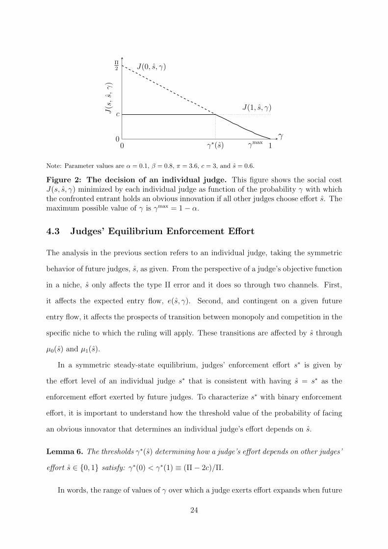
Proposition 2 (Screening complements enforcement). For any value of other judges’
enforcement effort s ∈ [0, 1]: i) If c < Π/2, there exists a threshold value for the probability
of facing an obvious innovator, γ∗(s) ∈ (0, 1) such that the judge exerts effort if and only
if γ ≤ γ∗(s). ii) If c ≥ Π/2, a judge does not exert effort regardless of the value of γ > 0.
The main implication of the previous proposition is that the patent office’s screening
rate (which reduces λ and hence γ) and an individual judge’s enforcement effort are
complementary. Intuitively, if the patent office screens out a larger proportion of obvious
innovations (lower λ), the social cost of making a judicial error increases (as it is more likely
to be type I error in this case), which encourages the judge to exert effort. Mathematically,
(17) decreases in γ both directly and indirectly through Φ(s, γ) as observed in Lemma 5.
Figure 2 illustrates the trade-offs behind this result. It depicts the social cost internal-
ized by an individual judge as a function of the probability of facing an obvious innovator,
γ, under the two possible enforcement effort choices, s = 0 and s = 1. The social cost
under full effort is flat and equal to c, whereas the social cost under no effort declines with
γ. The cutoff γ∗(s) separates the ranges of γ for which, given other judges’ enforcement
effort, an individual judge will or will not exert effort. The complementarity between
screening rate (low γ) and enforcement effort (choice of s = 1) will become important
when we characterize the equilibrium judge behavior.
In order to focus on the case in which full enforcement effort is possible in equilibrium,
throughout the rest of the paper we make the following assumption:
Assumption 2. c < Π/2.
23
0 1
J(0, s, γ)
J(1, s, γ)
γ∗(s) γmaxγ0
Π2
cJ(s
,s,γ
)
Note: Parameter values are α = 0.1, β = 0.8, π = 3.6, c = 3, and s = 0.6.
Figure 2: The decision of an individual judge. This figure shows the social costJ(s, s, γ) minimized by each individual judge as function of the probability γ with whichthe confronted entrant holds an obvious innovation if all other judges choose effort s. Themaximum possible value of γ is γmax = 1− α.
4.3 Judges’ Equilibrium Enforcement Effort
The analysis in the previous section refers to an individual judge, taking the symmetric
behavior of future judges, s, as given. From the perspective of a judge’s objective function
in a niche, s only affects the type II error and it does so through two channels. First,
it affects the expected entry flow, e(s, γ). Second, and contingent on a given future
entry flow, it affects the prospects of transition between monopoly and competition in the
specific niche to which the ruling will apply. These transitions are affected by s through
µ0(s) and µ1(s).
In a symmetric steady-state equilibrium, judges’ enforcement effort s∗ is given by
the effort level of an individual judge s∗ that is consistent with having s = s∗ as the
enforcement effort exerted by future judges. To characterize s∗ with binary enforcement
effort, it is important to understand how the threshold value of the probability of facing
an obvious innovator that determines an individual judge’s effort depends on s.
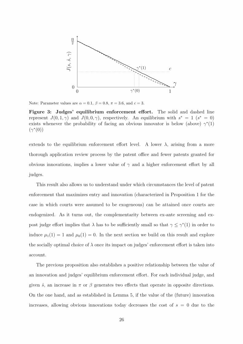
Lemma 6. The thresholds γ∗(s) determining how a judge’s effort depends on other judges’
effort s ∈ 0, 1 satisfy: γ∗(0) < γ∗(1) ≡ (Π− 2c)/Π.
In words, the range of values of γ over which a judge exerts effort expands when future
24

judges are also expected to exert effort, meaning that the effort of subsequent judges
are strategic complements. This result, illustrated in Figure 3, yields the equilibrium
configurations described in the next proposition.
Proposition 3 (Enforcement equilibria). In a pure-strategy symmetric steady-state equi-
librium, judges’ effort in the patent enforcement game is given by:
s∗ =
1 if γ ≤ γ∗(0),
0, 1 if γ ∈ (γ∗(0), γ∗(1)],
0 if γ > γ∗(1).
In the multiple equilibrium region, entry is higher with full enforcement effort (s∗ = 1)
than with no enforcement effort (s∗ = 0).
The underlying complementary implies that a choice s = 0 (s = 1) by other judges
strengthens the incentives for a given judge to also choose s = 0 (s = 1). With low effort
some obvious innovators will end up replacing existing monopolists, which contributes to
increase social welfare by facilitating the entry of future genuine innovators. However,
under s = 1 this entry-facilitating effect of s = 0 (and, thus, the convenience of the
type II error) disappears because future judges always allow genuine innovators to enter.
Without the rationale for s = 0 coming from the convenience of type II error, whether
s = 0 or s = 1 is optimal only depends on comparing the gains from reducing type I error
with the enforcement effort cost c.
We can now characterize how the equilibrium enforcement effort changes with the
parameters of the model.
Proposition 4 (Comparative Statics). In the symmetric steady-state equilibrium, judges’
enforcement effort s∗ is increasing in the value of a genuine innovation Π, increasing in the
screening quality of the patent office (decreasing in λ), and decreasing in the enforcement
effort cost, c.
In the previous section we established the complementarity between the effort carried
out by an individual judge and the ex-ante screening of patents. This result naturally
25
0 1
cγ∗(1)J(s
,s,γ
)
γ∗(0)
γ0
Π2
Note: Parameter values are α = 0.1, β = 0.8, π = 3.6, and c = 3.
Figure 3: Judges’ equilibrium enforcement effort. The solid and dashed linerepresent J(0, 1, γ) and J(0, 0, γ), respectively. An equilibrium with s∗ = 1 (s∗ = 0)exists whenever the probability of facing an obvious innovator is below (above) γ∗(1)(γ∗(0))
extends to the equilibrium enforcement effort level. A lower λ, arising from a more
thorough application review process by the patent office and fewer patents granted for
obvious innovations, implies a lower value of γ and a higher enforcement effort by all
judges.
This result also allows us to understand under which circumstances the level of patent
enforcement that maximizes entry and innovation (characterized in Proposition 1 for the
case in which courts were assumed to be exogeneous) can be attained once courts are
endogenized. As it turns out, the complementarity between ex-ante screening and ex-
post judge effort implies that λ has to be sufficiently small so that γ ≤ γ∗(1) in order to
induce µ1(1) = 1 and µ0(1) = 0. In the next section we build on this result and explore
the socially optimal choice of λ once its impact on judges’ enforcement effort is taken into
account.
The previous proposition also establishes a positive relationship between the value of
an innovation and judges’ equilibrium enforcement effort. For each individual judge, and
given s, an increase in π or β generates two effects that operate in opposite directions.
On the one hand, and as established in Lemma 5, if the value of the (future) innovation
increases, allowing obvious innovations today decreases the cost of s = 0 due to the
26

higher social value of type II error. On the other hand, the higher the discounted value of
the innovation, the higher the cost of mistakenly preventing the production of a genuine
innovation in the current period (type I error). When π or β increase, this second effect
dominates, implying an upward shift in the function J(0, s∗, γ) for both s = 0 and s = 1.
In terms of Figure 3 this means that both γ∗(0) and γ∗(1) increase, expanding the region
over which an equilibrium with s∗ = 1 is sustainable. As genuine innovations become more
prevalent (lower λ) and their social value increases (higher Π), investing in enhancing the
quality of enforcement becomes more valuable and an equilibrium with full enforcement
is more likely to emerge.17
4.4 Screening and Enforcement Equilibrium
In this section we characterize the socially optimal patent screening rate, λ∗, taking into
account the endogenous response of courts. Given the equilibrium enforcement effort
decision of judges, s∗(λ, c) characterized in the previous section, a social planner chooses
λ to maximize18
W (λ; s∗, c) = e (s∗, λ) [p (s∗, λ) Π− 1− κ(λ)− c(α + (1− α)λ)x (s∗, λ) s∗] (19)
where x (s∗, λ), p (s∗, λ) and, e (s∗, λ) are the equilibrium values for the proportion of
monopolized niches, the probability that an entrant obtains a novel innovation, and num-
ber of entrants, respectively (see equations (6), (7) and, (8)). Social welfare differs from
the patent’s office problem (10) in two ways. First, equation (10) is not regarded as the
endogenous enforcement effort of judges. Second, social welfare in (19) also takes into
account that judges incur in a cost of s∗(λ, c)c per case reviewed and that the mass of
cases reviewed is the proportion (α + (1− α)λ)x (s∗, λ) of entrants that obtain a patent
and land in a monopolized niche.
17The effect of α is more difficult to assess. It is true that, given γ, the cost of poor enforcementdecreases as α increases (see Lemma 5). However, the value of γ negatively depends on α. Numericalcalculations indicate that, as in the case of Π, the overall effect of α on s∗ is positive, although ananalytical characterization of this result is elusive.
18For parsimoniousness, we omit λ and c from s∗(λ, c) as arguments in equation (19).
27

To solve the previous problem it is convenient to define the socially optimal values of
λ conditional on each of the possible levels of judge-enforcement effort:
λ0 ∈ arg maxλ∈[0,1]
W (λ; s, c) , s.t. s∗(λ, c) = 0,
which does not depend on c, since when judges exert no effort this cost does not affect
social welfare, and
λ1(c) ∈ arg maxλ∈[0,1]
W (λ; s, c) , s.t. s∗(λ, c) = 1.
Finally, we define c01 to be the unique value of c that solves W (λ0; 0) ≡ W (λ1(c01); 1, c01);
that is, c01 is the maximum enforcement cost under which inducing judge effort might be
optimal.
To solve the planner’s problem, we make two simplifying assumptions. First, we
assume κ(λ) = (1 − λ)2/λ. Assuming a functional form allows us to simplify exposition
in the proof, but the proposition holds more generally. We also assume that λ1(c01) < λ0;
that is, when the enforcement cost is such that the optimal screening with and without
effort leads to identical welfare, better screening by the patent office is required when
judges exert effort.19
Proposition 5 (Optimal Screening). Assume κ(λ) = (1−λ)2/λ and λ1(c01) < λ0. Then,
there exists a threshold c∗ such that the socially optimal ex-ante patent screening rate,
λ∗(c), is decreasing in c and equal to λ1(c) (which induces full judge effort) whenever
c ≤ c∗, and equal to λ0 (which induces no effort) otherwise. Furthermore, λ∗(c) has a
upward discontinuity at c∗.
The previous result is illustrated in Figure 4. The social planner faces the following
tradeoff: a low screening level (high λ) saves on the cost of reviewing patent applications
by the patent office but reduces judges’ incentives to exert enforcement effort, so it is
only compatible with inducing such effort for when the enforcement cost c is low. As
19This assumption holds in every numerical simulation of the model under the adopted functional formfor κ.
28

0 c∗ = 0.79
1
λ∗
λ1(c)
λ0
c
Note: Parameter values are α = 0.1, β = 0.8, and π = 3.6.
Figure 4: Optimal screening as a function of the enforcement cost. As a resultof substitutability, screening increases (λ∗ declines) with the enforcement cost c while itis optimal to induce high enforcement effort by judges. When c > c∗, judges perform lowenforcement effort and, as a result of complementarities, screening jumps down (λ∗ jumpsto λ0).
c increases, the optimal patent screening increases (λso falls). Beyond the threshold c∗,
it is socially superior to give up on inducing a high level of enforcement. The upward
jump of λ∗ at c∗ (that is, the fall in screening at that point) reflects the complementarity
between ex-ante screening and ex-post enforcement. As explained in prior sections, the
lower screening rate removes some monopolies, replacing them with obvious innovators,
reducing the hurdle to future entry and mitigating the discouragement to innovation that
a low enforcement effort would otherwise generate. As we shall see below, the effects of
this complementarity also tend to prevail in the case in which we allow judges’ enforcement
effort to vary continuously.
5 Robustness and Extensions
Here we analyze two extensions of the main model and show that the main insights from
previous sections go through in alternative or more general settings. First, we study
how the existence of static inefficiency in a context of cost-saving innovations affects the
judges’ decisions and the outcome of the patent enforcement game. We then examine the
29

case in which judges’ enforcement effort is continuous. The technical details are relegated
to Appendix B.
5.1 Cost-saving Innovations and Static Inefficiency
In the baseline model we consider quality-improving innovations in an environment with
inelastic demands. In that context, genuine innovators extract all the surplus from con-
sumers, avoiding deadweight losses and simplifying the welfare analysis. We now provide
a tractable framework that extends our analysis to a case of cost-reducing innovations,
where market power involves welfare losses.
In this setup there is also a continuum of niches of size 1. In each niche the good
produced is homogeneous. Firms compete in prices and face a demand function q = a/p.
Each genuine innovation decreases the existing marginal cost by a proportion 1− δ where
δ ∈ (0, 1). That is, if z represents the baseline marginal cost, after m genuine innovations
the marginal cost becomes zm = δmz.20
Lemma 7. In a cost-saving innovations setup, the profit flow π and the deadweight loss
` generated by a genuine innovation are independent of the baseline marginal cost z and
the cumulative number of innovations m. In particular, as illustrated in Figure 5, they
are equal to π = a(1− δ) and ` = a (ln(δ−1)− (1− δ)) > 0.
Social Welfare Because profits are invariant to the cumulative number of innovations,
firm behavior and industry dynamics described in Section 3 go through without alter-
ations. The objective functions of the patent office and courts, however, need to be
reformulated to account for the deadweight loss `. In particular, the main difference with
respect to the baseline model is that now, allowing entry into a monopolized niche con-
verts the existing deadweight loss into consumer surplus. Entry, whether from a genuine
or obvious entrant, increases the social welfare by ` on a permanent basis, L ≡ `/(1− β).
20This demand and the proportional cost-saving innovation are also used in Marshall and Parra (2019).
30

p
q
z0
z1 = δz0
z2 = δ2z0
AB
C D E
π = A = C +D = a(1− δ)` = B = E = a
(ln(δ−1)− (1− δ)
)
q0 q1 q2
Figure 5: Monopoly profits and deadweight losses with cost-saving innova-tions. This figure identifies the profits (π) and deadweight losses (`) associated with asuccessful genuine cost-saving innovation as areas under the relevant demand curve.
As carefully shown in Appendix B.1. the objective function of the patent office is now
W = e [p(Π + L)− 1− κ(λ)] .
This expression is analogous to that in (10) except for the new term in L, which captures
the deadweight loss recouped with the arrival of an innovation. Because the behavior of
e and p with respect to λ remains unchanged with respect to the baseline model, it is
immediate that the message of Proposition 1 extends to this environment. When courts’
behavior, as represented by µ0 and µ1, is exogenous, the optimal patent screening rate
may be interior even in the absence of screening costs.
The Judges’ Problem We can now analyze how a judge’s enforcement decision changes
when innovations are cost reducing and monopoly involves a deadweight loss. Recall that
entry is only opposed by the incumbent in a monopolized niche. Therefore, a ruling in
favor of the entrant will always increase welfare by (at least) L regardless of the entrant’s
innovation quality. As in the benchmark case, a type I error arises whenever a genuine
innovation is excluded from the market. Since this error can only occur in already mo-
nopolized niches, it now leads to a loss of ECSI = Π +L, where the superindex CS stands
for the cost-saving innovation setup.
31

The cost of type II error represents the reduction (in fact a gain, since its sign is
negative as in the benchmark model) in social welfare that occurs when a firm with an
obvious innovation is allowed to replace an active monopolist. This error has now two
components. First, each time a monopolist is replaced by another firm, the deadweight
loss associated to its innovation is eliminated, leading to an immediate gain of L. Second,
as in the benchmark case, the dynamic effect of enhanced entry increases the future social
value of the niche. Altogether, the benefit of type II error is now larger compared to the
benchmark model; that is, for every s and γ, ECSII (s, γ) < EII(s, γ).
As before, an individual judge decides her enforcement effort s taking as given the en-
forcement effort decisions of other judges s. We denote as JCS(s, s, γ) the cost minimized
by the individual judge in this case. As in the benchmark case, when a judge chooses
s = 1 no error is made, so the only cost is that related to her effort, JCS(1, s, γ) = c.
When a judge chooses effort s = 0, however, the cost is
JCS(0, s, γ) = J(0, s, γ) + L(1− γ)∆(s, γ)/2,
where J(0, s, γ), defined in (17), is the judge’s loss function in the model without dead-
weight losses and
∆(s, γ) =(1− 2γ)(1− β) + αβ(1− γ)e(s, γ)
(1− γ)(1− β) + αβ (1− γ + γµ0(s)) e(s, γ)≤ 1
is a function which, given the effort of other judges and the level of screening by the
patent office, measures the net intertemporal contribution of type I and type II errors to
the occurrence of the deadweight losses represented by L.
Similarly to the factor Φ(s, γ) that measures the net detrimental impact of judicial
errors on the entry of genuine innovators, the factor ∆(s, γ) is decreasing in the probability
that the confronted entrant is an obvious innovator, γ, which implies that the presence
of the deadweight loss L reinforces the complementarity between patent screening (which
reduces γ) and patent enforcement (which avoids the cost JCS(0, s, γ)). Observe that, for
values of γ close to one ∆(s, γ) can be negative, whereas when γ is low ∆(s, γ) is positive.
The stronger dependence of JCS(0, s, γ) on γ explains the following result:
32

0 1
J(0, s, γ) JCS(0, s, γ)
ca
cb
J(s
,s,γ
)
γγ
0
Π2
Note: Parameter values are α = 0.1, β = 0.8, a = 4, δ = 0.1, ca = 5, cb = 1 and s = 1.
Figure 6: Costs minimized by an individual judge with and without staticinefficiency. The solid and dashed lines represent J(0, s, γ) and JCS(0, s, γ), respec-tively. The parallel dotted lines show two possible illustrative levels of the cost of highenforcement effort.
Proposition 6 (Enforcement incentives with deadweight losses). For every s ∈ [0, 1],
there exists γ(s) ∈ (0, 1), increasing in αΠ, such that: i) when γ > γ(s) a judge has
less incentives to exert effort relative to a situation without static inefficiency; ii) when
γ < γ(s) a judge has more incentives to exert effort relative to a situation without static
inefficiency.
Thus, as shown in Figure 6, whether a judge exerts more or less effort relative to the
model without deadweight losses depends on the values of γ and c. As in the baseline
case, provided c is not too large, the judge exerts effort if and only if γ is low enough.
For high values of the enforcement cost, such as ca, the range of values of γ leading to
maximum enforcement effort is wider in the situation with deadweight losses. But when
the cost is low enough, such as cb, the result is reversed and, in the presence of deadweight
losses, maximum effort prevails over a narrower set of values of γ.
From here, the final characterization of the possible outcomes of judges’ enforcement
game would be analogous to that in Proposition 3. Relative to the model without dead-
weight losses, the ranges of values of γ over which an equilibrium with high enforcement
33

effort can be sustained expand with c.
5.2 Continuous Enforcement Effort
From Section 4.2 onwards, we streamlined the analysis by focusing on the case in which
judge enforcement effort can take only two values, s ∈ 0, 1. In this section we explore the
case where effort is continuous, s ∈ [0, 1]. As expected, the main results carry through. To
ease the exposition, we assume that the cost of exerting effort is quadratic. In particular
c(s) = cs2/2 where c > 0 is a scale parameter. In line with Assumption 2 above, in this
section we focus on the case in which effort is interior, that is, c > Π/2. We provide
details for this case and for the case where c ≤ Π/2 in Appendix B.2.
For a given enforcement effort by other judges s and screening rate by the patent
office, γ, a judge’s best response is unique an given by
s(s, γ) = Π(1− γ)Φ(s, γ)/2c ∈ (0, 1)
where Φ(s, γ) is the function defined in Lemma 5. It also follows from this lemma that the
best response of an individual judge, s(s, γ), increases in the quality of the screening of the
patent office (decreases in γ). That is, ex-ante patent screening remains complementary
to ex-post enforcement under continuous enforcement effort.
Proposition 7 (Revisiting judges’ effort complementarity). In the continuous enforce-
ment effort case, a judge’s best response is increasing in the enforcement effort of other
judges s if and only if
Π >3− s− 2γ
α(1 + s(1− 2γ))(20)
This condition always holds in a neighborhood of s = 1 or γ = 1.
Proposition 7 shows that, unlike in the binary effort scenario, where judge enforce-
ment effort decisions are complementary, here judges’ enforcement efforts can be strategic
complements or strategic substitutes. An increase in other judges’ effort s induces two
opposing effects. As in the baseline model (see Lemma 2), the proportion of monopo-
lized niches increases, making the frequency of type I errors higher, relative to type II
34

0 0.2 0.4 0.6 0.8 1
0.32
0.34
0.36
s
s∗(s,γ
)
(a) Strategic complements (γ = 0.6)
0 0.2 0.4 0.6 0.8 10.65
0.66
0.67
s
s∗(s,γ
)
(b) Substitutes and complements (γ = 0.25)
Note: Parameter values are α = 0.1, β = 0.8, π = 3.6, and c = 14.
Figure 7: Complementarity in the continuous enforcement effort case. Panelsshow the best response of an individual judge to other judges’ enforcement effort s fortwo different levels of the screening by the patent office, as (inversely) measured by γ.In panel (a) judges’ efforts are strategic complements, while in panel (b) they can bestrategic substitutes or complements depending on the size of s.
errors. This effect increases the factor Φ(s, γ), calling for more effort, that is, pushing
for strategic complementarity. On the one hand, in the continuous effort scenario a new
free-riding effect arises. Better (but far from perfect) rulings by other judges increase the
probability of future successful entry, p(s, γ). The prospect of higher entry increases the
benefits of a type II error, decreasing Φ(s, γ) (see Lemma 5) and, through it, the effort of
an individual judge’s best response. This effect (which vanishes in the proximity of s = 1)
pushes towards strategic substitutability.
The necessary and sufficient condition (20) tells us that strategic complementarity
tends to occur when incumbency profits are sufficiently high. The condition becomes
weaker when the patent office screens less (higher γ) and when other judges exert more
effort (they are already making good rulings). Consistent with the binary effort case,
regardless of the parameters of the model, strategic complementarity always occurs when
other judges’ enforcement effort is high enough. Complementarity also occurs when the
patent office screens little and/or most innovations are obvious (that is, when γ is high);
see Figure 7a. In contrast, as depicted in Figure 7b, substitutability can emerge under
35

2 4 6 8 10 12 14
0.8
0.85
0.9
λ
λ∗
c
(a) Optimal screening
2 4 6 8 10 12 140
0.1
0.2
0.3
0.4
c
s∗(λ∗ )
(b) Optimal enforcement
Note: parameter values are α = 0.1, β = 0.8, and π = 3.6.
Figure 8: Optimal screening and induced level of enforcement in continuouseffort case. Panel (a) depicts optimal ex-ante screening when enforcement effort isendogenous and exogenous (λ∗ and λ, respectively), as a function of the enforcement costc. Panel (b) shows the enforcement effort s∗(λ∗) induced by the optimal ex-ante screeningquality λ∗, also as a function of c.
higher ex-ante screening.
In Appendix B we show that the multiplicity of equilibria in the enforcement game
is not present when judges’ enforcement effort is continuous. That is, there is a unique
symmetric steady-state equilibrium with an effort level s∗ satisfying s(s∗, γ) = s∗. This
means that, with continuous enforcement efforts, the judges’ enforcement game no longer
entails a coordination problem.21
To conclude this section we numerically explore the socially optimal screening (see
problem (19)) under continuous enforcement effort. Figure 8 shows a case in which,
consistent with the complementarity discussed in Proposition 5, an increase in the en-
forcement costs decreases both judges’ enforcement effort (panel (b)) and patent office’s
ex-ante screening (panel (a)). That is, despite the substitution effect calling for better
screening when the cost of enforcement goes up, the impact of a decrease in enforcement
21This suggests that the coordination problem in the binary efforts case is related to the manner inwhich the prospects of perfect enforcement by subsequent judges (s = 1) fully removes the social valueof type II error, reinforcing the incentive of an individual judge to choose s = 1. For s < 1, type II errorby an individual judge is still valuable at the margin.
36

effort dominates, inducing less screening in equilibrium.
To illustrate this complementarity in a different way, we also compare the socially
optimal ex-ante screening behavior λ∗, just described, with what would be the optimal
screening in the hypothetical case in which court behavior remains exogenously fixed at
the equilibrium value induced by λ∗, s∗(λ∗). We call the optimal screening rate in the
hypothetical scenario λ. As shown in Figure 8a, when courts’ endogenous responses are
taken into account, it is socially efficient to screen more (to set a lower λ): the possibility
to affect court’s behavior, induces more screening in equilibrium.
6 Concluding Remarks
Innovation is considered key to industry dynamics. Entry, exit, and innovation are com-
plex interrelated phenomena in every industry, and especially so in those that are youngest
and more technology-intensive. Many of these industries rely on IP as the source of tem-
porary monopoly power that allows the successful innovators to obtain a return from
their previous R&D investments. IP protection, however, is a double-edged sword for the
dynamics of innovative industries, as the protection of incumbent innovators may be an
obstacle to the success of genuine innovators.
This paper contributes to the growing literature that analyzes the role of IP protec-
tion by embedding it in an industry-dynamics framework in which the value of innovation
is stochastic and new firms replaced existing incumbents. We find that innovation and
welfare are maximized when incumbents receive maximal protection against small im-
provements but as little as possible against large innovations. However, if incumbents
receive some protection against large innovation, allowing for some small improvements
to succeed in the market may be socially beneficial.
We also delve into the interaction between the mechanisms that implement the level
of protection of incumbents against each kind of innovation, namely the ex-ante screening
of the patent office and the ex-post enforcement by courts. The patent office can expend
37

resources in trying to screen out small innovations before their very entry. Courts enter
the game once an incumbent claims that its IP has been infringed by an entrant and can
at that stage invest resources to improve the quality of their rulings. We show that courts
provide better enforcement the more the patent office engages in the ex-ante screening.
This complementarity shapes the choice of the socially optimal level of screening by the
patent office.
Our model focuses on the interaction between the patent office’s ex-ante screening and
courts’ enforcement of intellectual property but remains silent about other dimensions of
patent policy. Future work could extend this type of analysis to cover aspects such as
patent breadth or patentability standards, which until now have been studied in the
literature without accounting for judges’ endogenous enforcement decisions.
38

References
Aghion, Philippe and Peter Howitt, “A Model of Growth through Creative De-
struction,” Econometrica, 1992, 60 (2), pp. 323–351.
Allison, John R. and Mark A. Lemley, “Empirical evidence on the validity of
litigated patents,” AIPLA Quarterly Journal , 1998, 26 (3), p. 185.
Bessen, James and Eric Maskin, “Sequential Innovation, Patents, and Imitation,”
Rand Journal of Economics , 2009, 40 (4), pp. 611–635.
Daughety, Andrew F. and Jennifer F. Reinganum, “Keeping Society in the Dark:
On the Admissibility of Pretrial Negotiations as Evidence in Court,” Rand Journal of
Economics , 1995, 26 (2), pp. 203–221.
Daughety, Andrew F and Jennifer F Reinganum, “Appealing judgments,” Rand
Journal of Economics , 2000, 31 (3), pp. 502–525.
—, “Informal sanctions on prosecutors and defendants and the disposition of criminal
cases,” Journal of Law, Economics, and Organization, 2016, 32 (2), pp. 359–394.
—, “Reducing Unjust Convictions: Plea Bargaining, Trial, and Evidence Disclosure,”
Journal of Law, Economics, and Organization, 2020, 36 (2), pp. 378–414.
Denicolo, Vincenzo, “Two-Stage Patent Races and Patent Policy,” Rand Journal of
Economics , 2000, 31 (3), pp. 488–501.
Denicolo, Vincenzo and Piercarlo Zanchettin, “How should forward patent
protection be provided?” International Journal of Industrial Organization, 2002, 20 (6),
pp. 801–827.
Denicolo, Vincenzo and Piercarlo Zanchettin, “What Causes Over-investment
in R&D in Endogenous Growth Models?” Economic Journal , 2014, 124 (581), pp.
1192–1212.
Farrell, Joseph and Robert P. Merges, “Incentives to challenge and defend
patents: Why litigation won’t help reliably fix patent office errors and administra-
tive patent review might help,” Berkeley Technology Law Journal , 2004, 19 (3), pp.
943–970.
Farrell, Joseph and Carl Shapiro, “How Strong Are Weak Patents,” American
Economic Review , 2008, 98 (4), pp. 1347–1369.
39

Frakes, Michael D. and Melissa F. Wasserman, “Is the Time Allocated to Review
Patent Applications Inducing Examiners to Grant Invalid Patents? Evidence from
Microlevel Application Data,” Review of Economics and Statistics , 2017, 99 (3), pp.
550–563.
—, “Irrational Ignorance at the Patent Office,” Vanderbilt Law Review , 2019, 72 (3), pp.
975–1030.
Galasso, Alberto and Mark Schankerman, “Patents and cumulative innovation:
Causal evidence from the courts,” Quarterly Journal of Economics , 2015, 130 (1), pp.
317–369.
Gilbert, Richard J and David M G Newbery, “Preemptive Patenting and the
Persistence of Monopoly,” American Economic Review , 1982, 72 (3), pp. 514–526.
Green, Jerry R. and Suzanne Scotchmer, “On the Division of Profit in Sequential
Innovation,” Rand Journal of Economics , 1995, 26 (1), pp. 20–33.
Grossman, Gene M and Elhanan Helpman, “Quality Ladders in the Theory of
Growth,” Review of Economic Studies , 1991, 58 (1), pp. 43–61.
Grossman, Gene M and Michael L Katz, “Plea bargaining and social welfare,”
American Economic Review , 1983, 73 (4), pp. 749–757.
Heller, Michael A. and Rebecca S. Eisenberg, “Can Patents Deter Innovation?
The Anticommons in Biomedical Research,” Science, 1998, 280 , pp. 698–701.
Hopenhayn, Hugo, Gerard Llobet and Matthew Mitchell, “Rewarding Se-
quential Innovations: Prizes, Patents and Buyouts,” Journal of Political Economy ,
2006, 104 (6), pp. 1041–1068.
Landeo, Claudia M, Maxim Nikitin and Scott Baker, “Deterrence, lawsuits, and
litigation outcomes under court errors,” Journal of Law, Economics, & Organization,
2007, 23 (1), pp. 57–97.
Lee, Tom and Louis L Wilde, “Market Structure and Innovation: A Reformulation,”
Quarterly Journal of Economics , 1980, 94 (2), pp. 429–36.
Lei, Zhen and Brian D. Wright, “Why weak patents? Testing the examiner igno-
rance hypothesis,” Journal of Public Economics , 2017, 148 , pp. 43–56.
40

Lemley, Mark A and Bhaven Sampat, “Is the patent office a rubber stamp,” Emory
Law Journal , 2008, 58 , p. 181.
Lemley, Mark A and Carl Shapiro, “Probabilistic patents,” Journal of Economic
Perspectives , 2005, 19 (2), pp. 75–98.
Lemley, Mark D., “Rational Ignorance at the Patent Office,” Northwestern University
Law Review , 2001, 95 (1495-1532).
—, “Ignoring Patents,” Michigan State Law Review , 2008, pp. 19–34.
Loury, Glenn C, “Market Structure and Innovation,” Quarterly Journal of Economics ,
1979, 93 (3), pp. 395–410.
Marshall, Guillermo and Alvaro Parra, “Innovation and competition: The role
of the product market,” International Journal of Industrial Organization, 2019, 65 , pp.
221–247.
O’Donoghue, Ted, “A Patentability Requirement for Sequential Innovation,” Rand
Journal of Economics , 1998, 29 (4), pp. pp. 654–679.
O’Donoghue, Ted, Suzanne Scotchmer and Jacques-Francois Thisse,
“Patent Breadth, Patent Life, and the Pace of Technological Progress,” Journal of
Economics & Management Strategy , 1998, 7 (1), pp. 1–32.
Parra, Alvaro, “Sequential innovation, patent policy, and the dynamics of the replace-
ment effect,” Rand Journal of Economics , 2019, 50 (3), pp. 568–590.
Reinganum, Jennifer F, “Plea bargaining and prosecutorial discretion,” American
Economic Review , 1988, pp. 713–728.
Schankerman, Mark and Florian Schuett, “Patent Screening, Innovation, and
Welfare,” 2020, mimeo.
Scotchmer, Suzanne, Innovation and Incentives , MIT Press, Cambridge, MA, 2004.
Scotchmer, Suzanne and Jerry Green, “Novelty and Disclosure in Patent Law,”
Rand Journal of Economics , 1990, 21 (1), pp. pp. 131–146.
Segal, Ilya and Michael D. Whinston, “Antitrust in Innovative Industries,” Amer-
ican Economic Review , 2007, 97 (5), pp. 1703–1730.
41

Spier, Kathryn E, “Pretrial bargaining and the design of fee-shifting rules,” Rand
Journal of Economics , 1994, pp. 197–214.
Spier, Kathryn E., “Litigation,” in A. Mitchell Polinsky and Steven Shavell, eds.,
Handbook of Law and Economics , volume 1, Elsevier, 2007 pp. 259–342.
42

Appendix
A Proofs
Proof of Lemma 1. To show existence we start by imposing the steady conditionxt = x for all t in eq. (3), obtaining eq. (6). Replacing x into (4) we obtain eq. (7).Using the free-entry condition (5), we obtain v = p−1. Finally, using condition (5) againand in the steady state of (2), we find the expression for the entry flow (8). Because allthese equations are linear, we have a unique solution.
To determine when the entry flow is positive, observe that (8) is positive if and onlyif π > π and lower than one if and only if π < π + β[α + (1− α)λµ0]/α.
Proof of Lemmas 2 and 3. Most comparative statics are direct, as they follow fromdirect differentiation. The derivative of the entry flow with respect to λµ0 is
de
d (λµ0)=
(1− α) (1− β)
β (αµ1 + (1− α)λµ0)2
[1− Π
p2
α
](21)
where Π = π/(1− β) is the present social value of a genuine innovation. The sign of thederivative is given by the sign of the term in square brackets. This term is a monotonicallydecreasing function of Π. To show that the derivative can be positive for any value of λµ0,take the maximum value of Π for which there is no entry; i.e., take Π = π/(1− β) ≡ p−1.In this case, the bracket term becomes 1 − p/α, which is positive whenever µ1 < 1, asp < α. By continuity, the results holds for values of Π > p−1 for which there is entry.
To show that the derivative is negative when µ1 = 1, observe that in this case p = αand the parenthesis becomes 1 − Πα. In this scenario, Assumption 1 is equivalent toΠ > p−1 = α−1 and the derivative is negative for any value of λµ0. Finally, an exampleof an inverted-U shape relation is given in the main text.
Proof of Proposition 1. For an interior solution of λ we compute the derivative(11) under the assumption κ(λ) = 0 and solve for the values of λ such that (11) is equalto zero. Because the first order condition corresponds to a third degree polynomial, weobtain three candidate solution. Call them 0,−,+. The first solution,
λ0 =−α (Παµ1 − 1)
µ0 (1− α) (Πα− 1)< 0
where Π = π/(1 − β), corresponds to a value for which the welfare function is zero(W (λ0) = 0). This occurs as e(λ0) = 0 and p(λ0) = Π−1 hold. Using these facts, we showthat the second order condition at λ0 is positive. Start by observing
d2W
dλ2=d2e
dλ2(Πp− 1) + 2
de
dλ
dp
dλΠ + e
d2p
dλ2Π = 2
de
dλ
dp
dλΠ
Proposition 2 implies that dp/dλ > 0. Similarly, using p(λ0) = Π−1 and Assumption 1in (21) we can verify de/dλ > 0. Therefore, the critical point corresponding to a (local)minimum and a feasible maximum (i.e., with λ ∈ [0, 1]) must lie to the right of λ0.
The second and third solutions are given by
λ−,+ = λ0 +α (1− µ1)
(Πα±
√αΠ (Πα + 8)
)2µ0 (1− α) (Πα− 1)
43
Given Assumption 1, the denominator above is positive and the sign of the fractiondepends on solution. For the negative solution the numerator is negative, and positive forthe positive solution. Therefore, we have that λ− < λ0 < λ+. Thus, given the analysisabove, λ+ is the only feasible solution. It can be readily verified, through differentiation,that λ+ decreases in Π and that it is less than one whenever
Π ≤ K ≡ (α + (1− α)µ0)2
α(αµ1 + (1− α)µ0)(α(2µ1 − 1) + (1− α)µ0).
Finally, it can be verified that λ+ decreases in µ1 and λ+ < 0 when µ1 = 1. Consequently,there exists µ1 such that, µ1 > µ1 implies that λ = 0, which proves the result.
Proof of Lemma 4. Subtracting the value functions wM and wC we obtain
wM − wC = −eαΠ (1− µ1) + [1− e (α + (1− α)λµ0)] β(wM − wC),
Solving for wM − wC delivers (14).
Proof of Lemma 5. Fix a triplet (s, s, γ). Using EI = Π, EII given by equation (14),and equation (1) we can rewrite J (s, s, γ) as:
Π
2(1− γ) (1− s)
(1− γαβ (1− µ1 (s)) e (s, γ)
(1− β) (1− γ) + βα ((1− γ) + γµ0 (s)) e (s, γ)
)︸ ︷︷ ︸
Φ(s,γ)
+c (s) .
Working the parenthesis and using that µ0(s)+µ1(s) = 1 for all s, we obtain the expressionin (18). Differentiating Φ(s, γ) with respect to e (s, γ) we obtain
dΦ(s, γ)
de= − αβ (1− β) (1− γ) γµ0(s)
[(1− β) (1− γ) + βα ((1− γ) + γµ0) e (s, γ)]2< 0.
Because it will be useful for the comparative statics and to prove other propositions,we replace e (s, γ) (see equation (8)) into Φ(s, γ) to obtain
Φ (s, γ) =(1− γ) [Παk1 − k2] + k1k2
k2 (Παk1 − (1− µ1(s)) (1− γ))(22)
where k1 = (1− γ)µ1(s) + γµ0(s) and k2 = 1− γ + γµ0(s) are functions of s and γ. Weomit this dependence for parsimonious notation. Observe that, for a given γ, α and Πare always together in (22). Thus,
dΦ(s, γ)
dΠα= − γµ0(s)k2
1
k2(Παk1 − (1− µ1(s))(1− γ))2< 0
which proves the result for α and Π. Differentiating (22) with respect to γ we obtain
dΦ (s, γ)
dγ= −µ0
Παk1 (Παk1 − [k2 + (1− µ1(s)) (1− γ)]) + k22(1− µ1(s))
k22 (Παk1 − (1− µ1(s)) (1− γ))2 .
Observe that the denominator is always positive. Assumption 1 implies Π > k2/(αk1) =p−1. Because the numerator is increasing in Π, we can replace the minimal feasible profitin the numerator to obtain a upper bound for the derivative
dΦ (γ, s)
dγ< − γµ2
0 (1− µ1(s))
k2 (Παk1 − (1− µ1(s)) (1− γ))2 ≤ 0
44

which proves the last comparative statics result. Proof of Proposition 2. To show existence of γ∗(s) simply observe that, when γ = 0,J (0, s, 0) = Π/2. Also, when γ = 1, J (0, s, 1) = 0. Because J is continuous in γ,if c < Π/2, Intermediate Value Theorem implies there exists γ∗(s) ∈ (0, 1) such thatJ (0, s, γ∗(s)) = c. To prove that γ∗(s) is unique, we show that J (0, s, γ) is decreasing inγ. Computing the derivative of J (0, s, γ) with respect to γ we obtain
dJ (0, s, γ)
dγ=
Π
2
(−Φ (s, γ) + (1− γ)
dΦ (s, γ)
dγ
),
which, by Lemma 5, is negative. Thus, dJ/dγ < 0 and uniqueness follows. If c ≥ Π/2, Jdecreasing in γ implies that the cost of effort is always higher than no exerting effort.
Proof of Lemma 6. It can be readily verified that, when s = 1, Φ(1, γ) = 1. Conse-quently, solving for J(0, 1, γ) = c we obtain that γ∗(1) = (Π− 2c)/Π. Also, when s = 0,Φ(0, γ) < 1 for all γ > 0. Thus, J(0, 1, γ) > J(0, 0, γ) for all γ ∈ (0, 1). Starting fromγ∗(0) ∈ (0, 1). The previous observation implies c = J(0, 0, γ∗(0)) < J(0, 1, γ∗(0)). Then,because J is decreasing in γ (see Proposition 2), γ∗(0) < γ∗(1).
Proof or Proposition 3. The characterization of the equilibrium is immediate fromLemma 6 and the discussion in the text. Regarding the equilibrium entry, observe
e (0, γ) =2 (1− γ) (1− β)
αβ
(Πα
2− γ− 1
)e (1, γ) =
1− βαβ
(Πα− 1) .
If Π ≤ (2 − γ)/α, then e (0, γ) = 0 and e (1, γ) ≥ 0. If Π > (2 − γ)/α then e (0, γ) > 0and e(1) > e(0) if and only if
Π >(2− γ)
α
(2γ − 1)
γ.
Since (2γ − 1)/γ < 1 for γ < 1 and, in equilibrium, γ∗(s) < 1, the result holds.
Proof of Proposition 4. As explained in the main text the result arises from thecomplementarity of the decisions of individual judges. Hence, to conduct the comparativestatics exercise we only need to show that the effort level of a judge is monotonicallydecreasing in c and α and increasing in Π. The effect c is immediate, higher effort costsdecreases, on the margin, a judge’s effort. Regarding the effects of an increase in Π andα, we need to compute the sign of
dJ
dΠ=
1− γ2
(Φ + Π
dΦ
dΠ
)and
dJ
dα=
Π(1− γ)
2
∂Φ
∂α,
respectively. From Lemma 5 we know that Φ(s, γ) is decreasing in α for all s which isenough to show the effect of this parameter. For Π we have that
dJ
dΠ=
1− γ2
[(1− γ) (Παk1 − k2) + k1k2] [αΠk1 − (1− µ1(s))(1− γ)]− γµ0(s)Παk21
k2(Παk1 − (1− µ1(s))(1− γ))2,
where k1 and k2 are defined in Lemma 5. We show that a lower bound of this derivativeis positive. Notice that positive entry (assumption 1) implies that Π > k2/(αk1). As a
45
result both Παk1 − k2 > 0 and Παk1 − (1− µ1(s))(1− γ) > 0. This means that a lowerbound for the first square bracket is k1k2. Substituting and rearranging we obtain
dJ
dΠ>
(1− γ) [Παk21 − (1− µ1(s))k1k2]
k2(Παk1 − (1− µ1(s))(1− γ))2>
(1− γ)µ1(s)k1k2
k2(Παk1 − (1− µ1(s))(1− γ))2> 0,
where we used k2/(αk1) as a lower bound for Π, proving the result.
Proof of Proposition 5. For a given c, we want to solve λ∗(c) ∈ arg maxW sp(λ, c)where
W sp(λ, c) =
W (λ; 1, c) if λ ≤ λJ(c)
W (λ; 0) if λ > λJ(c)and λJ(c) =
α
1− αΠ− 2c
2c(23)
is the minimum screening quality that induces enforcement effort by the judges; λJ(c)comes from replacing γ∗(1) = (Π− 2c)/Π into equation (15). This function is decreasingin c, takes the value of zero when c = Π/2 and diverges when the enforcement costapproaches zero (see Figure 9).
0
λ
c
1
Π2
λJ(c)
λ1(c)
c1
λ0
c0
λ
c−1J (λ) c−1
1 (λ)
Figure 9: Enforcement effort constraint.
We need to find λ∗(c) and study howit changes with the cost of screening c. Tostart, we characterize the welfare functionunder no enforcement effort.
Lemma A.1. The function W (λ; 0) is sin-gle peaked when λ ∈ [0, 1].
Proof. Recall W (λ; 0) = e(λ)[Πp(λ) −1 − κ(λ)] and observe that W (1; 0) > 0and limλ→0W (λ, 0) = −∞. We showthat there is a unique λ0 ≥ 0 in thearg maxW (λ; 0) satisfying W (λ0; 0) > 0.The first order condition for an interiormaximum is given by
0 = e′(λ0) (Πp(λ0)− 1− κ(λ0)) + e(λ0) (Πp′(λ0)− κ′(λ0)) .
Observe that e(λ) and Πp′(λ)− κ′(λ) > 0 for all λ . Also, because W (0; 0) > 0, Πp(0)−1−κ(0) > 0 and, consequently, Πp(λ0)−1−κ(λ0) > 0 is necesary to have positive welfare.Thus, e′(λ0) < 0. The second order condition is given by
e′′(λ0) (Πp(λ0)− 1− κ(λ0)) + 2e′(λ0) (Πp′(λ0)− κ′(λ0)) + e(λ0) (Πp′′(λ0)− κ′′(λ0)) .
Substituting in Πp(λ0) − 1 − κ(λ0) = e(λ0) (Πp′(λ0)− κ′(λ0)) /(−e′(λ0)) from the firstorder condition, we obtain(
e′′(λ0)e(λ0)− 2e′′(λ0)2)
(Πp′(λ0)− κ′(λ0)) /(−e′(λ0)) + e(λ0) (Πp′′(λ0)− κ′′(λ0)) ,
which is negative, as Πp′′(λ)−κ′′(λ) < 0 and e′′(λ)e(λ)−2e′′(λ)2 < 0 for λ > 0. Therefore,every point satisfying the FOC is a maximum and, at most, one maximum exist. Thus,the function is single peaked in λ ∈ [0, 1] (where λ0 is either interior or 1).
46

We now turn to examine the scenario when judges exert full enforcement effort; thatis, we study the arg maxW (λ; 1, c), which has a unique solution, called λ1(c), implicitlygiven by the first order condition κ′(λ) = (1− α)c. Given the Inada conditions for κ(λ),the function λ1(c) is decreasing in c, takes the value of 1 when c = 0 and approaches zerofrom above as c goes to infinity.22 This implies that the functions λ1(c) and λJ(c) crossat least once.
Lemma A.2. If κ(λ) = (1 − λ)2/λ, then λ1(c) = 1/√
1 + c(1− α) and the functionsλ1(c) and λJ(c) single cross.
Proof. The functional form for λ1(c) follows from the first order condition. The problemλ1(c) = λJ(c) is cubic in c. Thus, it has three solutions, two of which are imaginary.Consequently, the functions cross only once in the real plane.
We define c1 to be the unique cost satisfying λ1(c1) = λJ(c1). The previous analysisimplies that λ1(c) < λJ(c) for all c < c1. Similarly, define c0 to be the unique costsatisfying λJ(c0) = λ0. The cost c0 can be above or below c1 (see Figure 9).
Lemma A.3. The function W (λ1(c); 1, c) is strictly decreasing in c and W (λJ(c); 1, c) isstrictly decreasing in c whenever c ≥ c1.
Proof. For W (λ1(c); 1, c), using the Envelope Theorem, we have
dW
dc= −(α + (1− α)λ1(c)) < 0.
For W (λJ(c); 1, c), differentiate with respect c to obtain
dW
dc= − (κ′(λJ(c)) + c(1− α))
dλJ(c)
dc− (α + (1− α)λJ(c))
Because c ≥ c1, we know λJ(c) ≤ λ1(c) and, consequently, 0 < −κ′(λ1(c)) ≤ −κ′(λJ(c)).Then, 0 = − (κ′(λ1(c)) + c(1− α)) ≤ − (κ′(λJ(c)) + c(1− α)) and the result follows fromobserving dλJ/dc < 0.
Lemma A.4. There is a unique cost c01 > 0 such that W (λ1(c01); 1, c01) = W (λ0; 0).Consequently, W (λ1(c); 1, c) > W (λ0; 0) for c < c01 and W (λ1(c); 1, c) < W (λ0; 0) ifc > c01.
Proof. It can be readily verified that, when c = 0, W (λ1(0); 1, 0) > W (λ0; 0). Then,because the function W (λ1(c); 1, c) is strictly decreasing in c and limc→∞W (λ1(c); 1, c) =−∞, there is a unique value of c, call it c01, such that W (λ1(c01); 1, c01) = W (λ0; 0) .
Figure 10 shows, in solid lines, W (λ1(c); 1, c) when c is 0 and c01, and W (λ, 0). Thevalues of λ0 and λ1(c01) are also depicted. Define c−1
1 (λ) to be the inverse of λ1(c). Thedashed line going through the points A and B depicts the pairs (λ,W (λ; 1, c−1
1 (λ))); thatis, the line shows the maximum welfare attainable when judges exert full effort and thescreening costs c−1
1 (λ) is such that λ is the optimal screening quality. It is clear that,without the constraint of λJ(c), the optimal screening quality λ∗(c) would be equal toλ1(c) for c ≤ c01 and equal to λ0 otherwise. To solve for the socially optimal screeningrate we need to study three cases: whether λJ(c01) is below, in, or above the interval[λ1(c01), λ0] (which is non-empty by assumption).
22Using implicit differentiation we obtain λ′1(c) = −(1− α)/κ′′(λ1(c)) < 0.
47
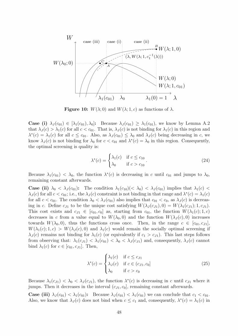
W (λ; 1, 0)
W (λ; 0)
W (λ; 1, c01)
λ
W
λ1(c01) λ0 λ1(0) = 1
W (λ0; 0)
(λ,W (λ; 1, c−11 (λ)))
case (i)case (iii) case (ii)B
A
C
Figure 10: W (λ; 0) and W (λ; 1, c) as functions of λ.
Case (i) λJ(c01) ∈ [λ1(c01), λ0]: Because λJ(c01) ≥ λ1(c01), we know by Lemma A.2that λJ(c) > λ1(c) for all c < c01. That is, λJ(c) is not binding for λ1(c) in this region andλ∗(c) = λ1(c) for all c ≤ c01. Also, as λJ(c01) ≤ λ0 and λJ(c) being decreasing in c, weknow λJ(c) is not binding for λ0 for c < c01 and λ∗(c) = λ0 in this region. Consequently,the optimal screening is quality is:
λ∗(c) =
λ1(c) if c ≤ c10
λ0 if c > c10
. (24)
Because λ1(c01) < λ0, the function λ∗(c) is decreasing in c until c01 and jumps to λ0,remaining constant afterwards.
Case (ii) λ0 < λJ(c01): The condition λ1(c10)(< λ0) < λJ(c01) implies that λ1(c) <λJ(c) for all c < c01; i.e., the λJ(c) constraint is not binding in that range and λ∗(c) = λ1(c)for all c < c01. The condition λ0 < λJ(c01) also implies that c01 < c0, as λJ(c) is decreas-ing in c. Define cJ1 to be the unique cost satisfying W (λJ(cJ1), 0) = W (λ1(cJ1); 1, cJ1).This cost exists and cJ1 ∈ [c01, c0] as, starting from c01, the function W (λ1(c); 1, c)decreases in c from a value equal to W (λ0, 0) and the function W (λJ(c), 0) increasestowards W (λ0, 0), thus the functions cross once. Then, in the range c ∈ [c01, cJ1],W (λ1(c); 1, c) > W (λJ(c), 0) and λ1(c) would remain the socially optimal screening ifλJ(c) remains not binding for λ1(c) (or equivalently if c1 > cJ1). This last steps followsfrom observing that: λ1(cJ1) < λ1(c01) < λ0 < λJ(cJ1) and, consequently, λJ(c) cannotbind λ1(c) for c ∈ [c01, cJ1]. Then,
λ∗(c) =
λ1(c) if c ≤ cJ1
λJ(c) if c ∈ (cJ1, c0]
λ0 if c > c0
(25)
Because λ1(cJ1) < λ0 < λJ(cJ1), the function λ∗(c) is decreasing in c until cJ1 where itjumps. Then it decreases in the interval (cJ1, c0], remaining constant afterwards.
Case (iii) λJ(c01) < λ1(c01): Because λJ(c01) < λ1(c01) we can conclude that c1 < c01.Also, we know that λJ(c) does not bind when c ≤ c1 and, consequently, λ∗(c) = λ1(c) in
48

that interval. Because c1 < c01, at or in a neighborhood of c1 we have W (λJ(c); 1, c) >W (λ0; 0). By Lemma A.3, we know that the function W (λJ(c); 1, c) is decreasing in cfor c > c1 and diverges to −∞ when the enforcement cost is unboundedly large. Thus,W (λJ(c); 1, c) single crosses W (λ0; 0). Define c0J to be such cost. We show that c0J >c0. Define c−1
J (λ) to be the inverse of λJ(c); i.e., for any λ and c such that λJ(c) =λ we have W (λ; 1, c−1
J (λ)) = W (λJ(c); 1, c). Then observe that, for any λ < λJ(c1),W (λ; 1, c−1
J (λ)) > W (λ; 1, c−11 (λ)) as, by construction, c−1
J (λ) < c−11 (λ) (see Figure 9).
Then,
W(λ1(c01); 1, c−1
J (λ1(c01)))> W
(λ1(c01); 1, c−1
1 (λ1(c01)))
= W (λ0; 0)
and, because W (λJ(c); 1, c) decreasing in c for c > c1 implies W (λ; 1, c−1J (λ)) increasing
in λ, the function W (λ; 1, c−1J (λ)) crosses W (λ0; 0) at a λJ(cJ0) < λ1(c01) < λ0; i.e., to
the left of point A in Figure 9 (e.g., point C). Consequently, c0J > c0. Then,
λ∗(c) =
λ1(c) if c ≤ c1
λJ(c) if c ∈ (c1, c0J ]
λ0 if c > c0J
(26)
Because λJ(c0J) < λ1(c01) < λ0, the function λ∗(c) is decreasing in c until c0J where itjumps to λ0, remaining constant afterwards.
Proof of Lemma 7. Let m > 1 be an arbitrary number of innovations in the qualityladder and zm = δmz for any z > 0. In a monopolized niche, due to the unit elasticity ofdemand, the incumbent wants to charge the highest price feasible. In this case p = zm−1.Then, the incumbent profits are given by π = (p− zm)q = a(1− δ) which is independentof the number of innovations and the baseline cost z. The dead-weight loss in the marketis given by ∫ zm−1
zm
q(p)dp− π = a(ln(δ−1)− (1− δ)
)also independent of m and z.
Proof of Proposition 6. Because sCS(s, γ) = s∗(s, γ) + (1− γ)L∆(s, γ)/2c and L > 0,whether sCS is higher than s∗ depends on the sign of ∆(s, γ). It is easy to verify that∆(s, 0) = 1 and limγ→1 ∆(s, γ) = −∞. Because ∆(s, γ) is strictly decreasing in γ andis continuous, ∆(s, γ(s)) = 0 exists and is uniquely defined. To show that γ(s) isincreasing in Πα, observe that
d∆
dΠα=
γk21[(1− γ)(1− µ0(s)) + γµ0(s)]
(1− γ)k2 [Παk1 − (1− µ1(s)))(1− γ)]2> 0.
Thus, because ∆(s, γ) is decreasing in γ, higher Πα implies a higher γ(s).
Proof of Proposition 7. Differentiating s∗(s, γ) with respect to s we obtain
dΦ
ds=
2γ (1− γ) k1
(k1 + s+ 2γ − 3
)k2
2
(k1 − (1− γ) (1− s)
)2 (27)
49

where k1 = Πα(1 + s (1− 2γ)) > 0 and k2 = 2 − γ (1 + s) > 0 are the analogousexpressions for k1 and k2 in Lemma 5 after replacing for the judge’s beliefs using (1).To ease out notation, k1 also includes Πα. The sign of this derivative is given by theterm in parenthesis in the numerator, which is positive if and only if condition (20) holds.When s = 1 or γ = 1 condition (20) becomes equal to Π > p(s, γ)−1 which is equivalentto the positive entry assumption (Assumption 1).
50

B Extensions: Technical Details
B.1 Cost-saving Innovations and Static Inefficiency
In this appendix we present the details of the cost-saving innovation model introduced inSection 5.1. We start deriving the objective function for the patent office and then moveto the judges’ problem.
Social Welfare Because profits are invariant to the cumulative number of innovations,the firm behavior and industry dynamics described in Section 3 go through without al-terations. The objective functions of the social planer and courts, however, need to bereformulated to account for the deadweight loss `. Figure 5 depicts the product marketpayoff associated with each innovation. Building on the expression for the deadweightlosses obtained in Lemma 7, social welfare can be written as follows
W = e(s, γ(λ))[(1− α)λxµ0(s)L+ α
(xµ1(s)(Π + L) + (1− x)Π
)− 1− κ(λ)
], (28)
where L ≡ `/(1 − β) is the present value of a permanent dead-weight loss. Notice thatin e(s, γ(λ)) we are making explicit the dependence of γ on λ (see equation (15)). Toexplain this welfare expression consider Figure 5 when the latest technology availablein the market attains a marginal cost z1. The first term in square brackets captures thearrival of an obvious entrant, which occurs with probability 1−α and who obtains a patentwith probability λ. With probability 1 − x the obvious entrant lands in a competitiveniche, not affecting welfare. With probability x the obvious entrant lands in a monopolizedniche and the incumbent takes it to court. The obvious entrant succeeds with probabilityµ0, in which case, the market price goes down from z0 to z1. The area A depicts theprofits of the replaced incumbent which are transferred to consumers as surplus. Thearea A brings no new social surplus. The area B, on the other hand, is the dead-weightloss associated with the patent protection given to the incumbent. With the arrival of theobvious innovation, this loss is transferred to consumers permanently, increasing welfareby L.
The second term in the expression represents the payoffs when the entrant is a genuineinnovator and obtains a patent, which occurs with probability α. With probability x theentrant lands in a monopolized niche and gets challenged in court. The entrant wins incourt with probability µ1. In that case, the price goes down from z0 to z1. As before,the area A is transferred from the incumbent to consumers and the original dead-weightloss, B, is now captured by consumers permanently. In contrast, the entrant capturesthe area C + D as profits. When a new innovation arrives in the future, these profitswill be eventually transferred to consumers. That is, the welfare value created are theareas B + C + D at perpetuity, or Π + L. Finally, when the genuine innovator landsin a competitive niche (that is, the existing price equals the marginal cost of the latesttechnology z1), it does not get challenged in court and appropriates the area C + D asprofits. As before, these profits will eventually be transferred to consumers when a newinnovation arrives. The entrant, thus, creates a welfare value Π. The area E is the newdeadweight loss created, not appropriated by anyone until a new innovation successfullyenters the market.
51

0 0.2 0.4 0.6 0.80.04
0.06
0.08
0.1
0.12·10−2
λµ0
W
Note: Parameter values are α = 0.1, π = 2.4, ` = 0.13 (i.e., a = 24 and δ = 0.9), β = 0.8 and µ1 = 0.85.
Figure 11: Welfare with deadweight loss; interior maximum when screening is free.
In order to understand better the welfare trade-offs in this model we can re-arrange(28) using the steady-state values of relevant objects provided in Lemma 1 we obtain
W = e [p(Π + L)− 1− κ(λ)] ,
which is the expression presented in the main text. Figure 11 presents an example of aninterior screening rate by the patent office when screening is free and the courts’ behavioris exogenous.
The Judges’ Problem We now analyze how a judge’s endogenous decision changeswhen innovations are cost reducing and a dead-weight loss might arise. As explainedin the main text a type I error arises whenever a genuine innovator is prevented fromentering the market. In this scenario the type I error leads to a loss ECS
I = Π + L.The type II error represents the “loss” in social welfare when a firm with an obvious
innovation is allowed to replace an active monopolist. This negative cost has now twocomponents. First, there is a short run gain, derived from eliminating the deadweightloss that the incumbent generated. Second, there is the same dynamic effect explained inthe benchmark case that increases the future value of the niche. That is,
ECSII = −L+ β(wCSM − wCSC ),
where the value of a monopolistic and competitive niche are respectively defined as
wCSC = βwC + e(s, γ(λ)) [α (Π + β(wM − wC))− 1] ,
wCSM = βwM + e(s, γ(λ)) [αµ1(s)(Π + L) + (1− α)λµ0(s) (L+ β(wC − wM))− 1] .(29)
The difference with the benchmark case is that, now, the value of a monopolistic nichedepends on the dead-weight loss L. Each time a monopolist is replaced by another firmthe deadweight loss associated to its innovation is eliminated and a discounted surplus
52

L is transferred to consumers by means of a lower price. This effect increases wM andnarrows the difference between the value of a monopolistic and a competitive niche.
As a result, the introduction of a deadweight loss generates two opposing effects on thetype II error. First, there is the static gain of eliminating the deadweight loss, enhancingthe return from eliminating an existing monopolist; i.e., making the type II error morenegative. The second effect, corresponds to the dynamic effect of reducing the incrementalvalue of a competitive niche relative to a monopolized one (discussed in the previousparagraph). As the next lemma shows, the static effect dominates.
Lemma B.1. For all s and γ, ECSII (s, γ) < EII(s, γ) where EII(s, γ) is given by (14) and
ECSII (s, γ) = EII(s, γ)− L (1− γ)[(1− β) + αβ(1− µ1(s))e(s, γ)]
(1− β)(1− γ) + αβ(1− γ + γµ0(s))e(s, γ).
Proof. Subtracting the value functions wM and wC in (29) and solving we obtain
β(wM − wC) =[β(αµ1(s) + (1− α)λµ0(s))L− α(1− µ1(s))Π]e(s, γ)
1− β + β(α + (1− α)λµ0(s)e(s, γ)
= Lβ(αµ1(s) + (1− α)λµ0(s))e(s, γ)
1− β + β(α + (1− α)λµ0(s)e(s, γ)+ EII ,
where (14) was used in the last step. Replacing in ECSII = −L+ β(wM −wC) delivers the
expression in the lemma. We now formalize the details of the analysis presented in the main text for an individual
judge’s decision. Recall that when a judge chooses s = 1 no error is made, so the onlycost is that related to her effort, JCS(1, s, γ) = c. When a judge chooses effort s = 0,however, the cost is
JCS(0, s, γ) = J(0, s, γ) + L(1− γ)∆(s, γ)/2,
where J(0, s, γ) is defined in (17) and
∆(s, γ) =(1− 2γ)(1− β) + αβ(1− γ)e(s, γ)
(1− γ)(1− β) + αβ (1− γ + γµ0(s)) e(s, γ)≤ 1. (30)
Proposition B.1 (Complementarity in the model with DWL). For a given s, ∆(s, γ) isdecreasing in γ. Consequently, JCS(0, s, γ) is decreasing in γ. That is, the presence ofthe term in L in JCS reinforces the negative effect of γ on the best response function ofan individual judge.
Proof. From Proposition 2 we know that J(0, s, γ) decreases in γ. We need to show that∆(s, γ) decreases in γ. Start by substituting for e(s, γ) in (30) to obtain
∆(s, γ) = Φ(s, γ)− Ω(s, γ), where Ω(s, γ) =γk1
(1− γ)[Παk1 − (1− µ1(s))(1− γ)],
Φ(s, γ) is given by (18), and k1 and k2 are defined in the proof of Lemma 5. By Lemma5, Φ(s, γ) decreases in γ. Hence, it is sufficient to show that Ω(s, γ) increases in γ.Differentiating
dΩ
dγ=
Παk21 − (1− µ1(s))(1− γ) (k1 + γµ0(s))
(1− γ)2 [Παk1 − (1− µ1(s)))(1− γ)]2.
53

The denominator is always positive. We use Assumption 1 (i.e., Π ≥ k2/(αk1)) to con-struct the following lower bound for the numerator
k1k2 − (1− µ1(s))(1− γ) (k1 + γµ0(s)) = γµ0(s)(1− γ)(4− 5µ0(s)) + (γ + µ0(s)− 1)2
where we have used µ1(s) = 1−µ0(s). This expression is positive as µ0(s) ≤ 1/2 for all s;proving that the derivative is positive. Therefore, ∆(s, γ) and, consequently, JCS(0, s, γ)decrease in γ.
B.2 Continuous Enforcement Effort
We previously assumed that a judge’s effort, s, could take only two values. The judgecould either exert no effort, 0, or full effort, 1. In this section we explore the case whereeffort is continuous; i.e., s ∈ [0, 1]. As expected, the main results carry through.
To ease the exposition, we assume that the cost of exerting effort is quadratic. Inparticular c(s) = cs2/2 where c > 0 is a scale parameter.23 Building on Lemma 5, theobjective function that a judge minimizes with respect s ∈ [0, 1] can be written as
J(s, s, γ) = Π(1− γ)(1− s)Φ(s, γ)/2 + c(s), (31)
where Φ(s, γ) ∈ (0, 1] is given by equation (18). This objective function is the continuous-effort analogous of (17). The next lemma characterizes an individualjudge’s best responsetaking the possibility of corner solutions into account.
Lemma B.2. For a given enforcement effort by other judges s and screening rate by thepatent office, γ, a judge’s best response is unique an given by
s(s, γ) = min 1,Π(1− γ)Φ(s, γ)/2c . (32)
If c > Π/2, the best response is always interior; i.e., s(s, γ) ∈ [0, 1). If c ≤ Π/2 thereexists values of (s, γ) for which the best response is s(s, γ) = 1.
Proof. The proof that s∗(s, γ) is interior whenever Π/2 < c was given in the main text.This solution is a minimum, as the second order condition is given by c > 0. For the casein which Π/2 ≥ c, take γ = 0. Then, (1 − γ)Φ(s, γ) = 1 and the first order condition ofthe judge’s problem (31) satisfies cs−Π/2 < 0 for all s ∈ [0, 1). Thus, s∗(s, 1) = 1 is theunique solution to the minimization problem.
The objective function in (19) is strictly convex so when s(s, γ) is interior it charac-terizes the unique solution of the judge’s problem. Additionally s(s, γ) is always positiveso the only corner solution that may arise involves s(s, γ) = 1. When the cost of effortis sufficiently high, c > Π/2, s∗(s, γ) < 1 for all values of (s, γ). To see this observe thatΠ/2c < 1 and, by Lemma 5, (1− γ)Φ(s, γ) ≤ 1.24 When the cost of effort is not too high,c < Π/2, the corner solution s(s, γ) = 1 arises for values of (s, γ) that make (1−γ)Φ(s, γ)sufficiently close to one.
In the rest of this section we focus on the case c > Π/2 so that the solution isguaranteed to be interior. This assumption is analogous to Assumption 2 in the binaryeffort scenario.
23Results can be easily generalized to an environment with a convex cost function (i.e., c′(s) > 0, c′′(s) >0 for s > 0) satisfying c(0) = c′(0) = 0.
24Under a general cost function c(s), the sufficient condition for an interior solution is c′(1) > Π/2.
54

Proposition B.2 (Screening complements enforcement). For a given screening rate bythe patent office γ, there is a unique symmetric steady-state equilibrium in the enforcementgame in which judges’ effort is s∗ such that s(s∗, γ) = s∗. In this equilibrium, an increasein the patent office’s quality of screening increases judges’ enforcement effort s∗. Thus,patent screening and patent enforcement are complementary.
Proof. For a given γ, a symmetric interior equilibrium is given by
s∗ = Π (1− γ) Φ (γ, s∗) /2c.
We prove that the symmetric equilibrium is unique. Define the function F (s, γ) =Π (1− γ) Φ (γ, s) /2 − cs. Every symmetric equilibrium is a solution to F (s∗, γ) = 0.To prove uniqueness, we show that dF/ds is negative; thus, for a given γ, F can onlycross zero once. Differentiating
dF
ds=
Π (1− γ)
2
dΦ
ds− c ≤ Π
2
((1− γ)
dΦ
ds− 1
).
where dΦ/ds is given by (27). The inequality above follows from the assumption c > Π/2.We show that an upperbound of the parenthesis in the expression above is negative. Theparenthesis is equal to
k1
[k1
(2γ (1− γ)2 − k2
2
)+ 2 (1− γ)
(γ (1− γ) k3 + k2
2 (1− s))]−(k2(1− γ)(1− s)
)2
k22
(k1 − (1− γ) (1− s)
)2
where k3 = s+2γ−3 < 0, and k1 and k2 are defined in the proof of Proposition 7. Becausethe denominator is positive, we need to show that an upperbound of the numerator isnegative. The last term of the numerator is a subtracting a positive term. Thus, it issufficient to show that the term in square brackets is non-positive. The first term of thesquare brackets, 2γ (1− γ)2 − k2
2, is negative. This can be readily verified using that k2
decreases in s. The second term of the square brackets is positive. Thus, the squarebrackets can be positive or negative. Using Assumption 1, we can use that the positiveentry assumption implies k1 > k2, to find the following upper bound for the term in squarebrackets
k1
(2γ (1− γ)2 − k2
2
)+ 2 (1− γ)
(γ (1− γ) k3 + k2
2 (1− s))<
−(2γ (1− γ)3 (1− s) + (2− γ (s+ 1))2 ((1− s) γ + 2s (1− γ))
)< 0
Therefore, dF/ds < 0 and the symmetric equilibrium is unique.To prove that the Patent office’s effort is complementary to a Judge’s effor we use the
Implicit Function theorem; i.e.,ds∗
dγ= −dF/dγ
dF/ds.
Observe that dF/dγ = dJ/dγ. From the proof of Proposition 2 we know dJ/dγ < 0.Consequently, we have that ds∗/dγ < 0, proving the result.
55

Proposition B.2 shows the robustness of the complementarity found in the case withbinary enforcement effort. Better patent screening (a decrease in γ) increases the enforce-ment effort exerted by the judges. It is also interesting to observe that the multiplicity ofequilibria is not present in this case. Specifically, with continuous enforcement efforts andafter ruling out corner solutions with s∗ = 1, we no longer have a coordination problemamong judges.25 Figure 8 depicts the equilibrium under various parameters and screeningrates. The upper left panel shows the complementarity between patent screening andpatent enforcement. The other two figures show how the equilibrium enforcement effortincreases in Π and α.
25This suggests that the coordination problem in the binary efforts case is related to the manner inwhich the prospects of perfect enforcement by subsequent judges (s = 1) fully removes the social valueof type II error, reinforcing the incentive of an individual judge to choose s = 1. For s < 1, type II errorby an individual judge is still valuable at the margin.
56