on the influence of coregistration errors on satellite...
TRANSCRIPT
A thesis submitted in partial fulfillment
for the degree of Bachelor of Engineering
On the influence of coregistration errors
on satellite image pansharpening methods
by Maximilian Langheinrich
Degree program: Geoinformatics and satellite positioning
Supervisors:
Prof. Dr. Peter Krzystek (University of Applied Sciences, Munich)
Dr. Tobias Storch (German Aerospace Agency)
In cooperation with:
Department Photogrammetry and Image Analysis
Remote Sensing Technology Institute, German Aerospace Center
Winter semester 2013/2014
Closing date: 05.05.2014

Acknowledgements
Very much gratitude to Prof. Dr. Peter Krzystek (University of Applied
Sciences Munich) and Dr. Tobias Storch (German Aerospace Center) for supervising
my thesis. I also want to thank the whole staff of the Remote Sensing Technology
Institute for supporting me with scientific advice and cake and enabling me a very
enjoyable time at the German Aerospace Center.
i

Attachments
ii
Contents
Acknowledgements i
Attachments ii
1 Introduction 1
1.1 Objectives of thesis . . . . . . . . . . . . . . . . . . . . . . . . . . . . 2
1.2 State of the art . . . . . . . . . . . . . . . . . . . . . . . . . . . . . . 2
1.3 Main results of thesis . . . . . . . . . . . . . . . . . . . . . . . . . . . 3
1.4 Structure of thesis . . . . . . . . . . . . . . . . . . . . . . . . . . . . 3
2 Optical remote sensing data 4
3 Pansharpening methods 10
3.1 GIHS . . . . . . . . . . . . . . . . . . . . . . . . . . . . . . . . . . . 10
3.2 SCFF . . . . . . . . . . . . . . . . . . . . . . . . . . . . . . . . . . . 12
4 Experiments 17
4.1 Quality metrics . . . . . . . . . . . . . . . . . . . . . . . . . . . . . . 17
4.2 Quality assessment . . . . . . . . . . . . . . . . . . . . . . . . . . . . 20
4.3 Computing performance . . . . . . . . . . . . . . . . . . . . . . . . . 29
5 Discussion 30
5.1 The influence of co-registration errors on pansharpening methods . . 30
5.2 Higher-level processing issues . . . . . . . . . . . . . . . . . . . . . . 38
5.2.1 Atmospheric correction . . . . . . . . . . . . . . . . . . . . . 38
5.2.2 Index application . . . . . . . . . . . . . . . . . . . . . . . . . 40
5.2.2.1 NDVI and EVI . . . . . . . . . . . . . . . . . . . . . 41
6 Conclusion 45
Bibliography 47
iii
Chapter 1
Introduction
Since the advent of remote sensing it has evolved into a broad field of research,
contributing to many sciences and commercial applications. The number of active
Earth observation satellites and new sensor technologies steadily grows and one of
the permanently most pursued aims is surely the enhancement of ground resolution.
Modern imaging satellites are able to provide images with a sub-meter ground sam-
pling distance. GeoEye-1 as the currently best performing operational commercial
satellite delivers a resolution of 0.41 m (although the data is typically downgraded
to 0.5 m due to US-American export regulations). In the near future projects like
WorldView 3 will be able to acquire images with an even higher resolution of 0.31 m.
On the other hand the development of platforms featuring a high spectral resolution,
like e.g. the upcoming EnMAP satellite (observing with 232 spectral bands), is an
important necessity in regard to the improvement of remote sensing applications.
Sensors capable of obtaining data with a high geometric resolution come with
the drawback of lacking detailed spectral information. Their relative reflective re-
sponse functions usually cover the visible and near infrared spectrum of light, referred
to as panchromatic spectrum, realized as a gray value intensity image of the Earth’s
surface. Sensors able to distinguish between multiple bands of wavelengths, so called
multi-spectral and hyper-spectral instruments, on the contrary, have a lower spatial
resolution, due to engineering implementation and physical constraints.
As remote sensing applications ideally use images featuring both, a high ge-
ometric and spectral resolution, many efforts have been made over the past three
decades to develop and enhance techniques to fuse panchromatic and multi-spectral
data into one high resolution multi-band image. Supported by the increasing per-
formance of computers, knowledge in the field of computer vision and the fact that
Earth observation platforms nowadays typically carry both types of above mentioned
1
Chapter 1 Introduction 2
sensors, many effective methods evolved. The technical term for fusion processes of
this kind is generally known as pansharpening.
1.1 Objectives of thesis
The aim of the on hand thesis, besides giving a small overview of commonly used
pansharpening methods, is to address the implicit problems of satellite image fusion,
especially those generated by potentially defective input data due to technical issues
and/or deficient calibration and processing of the underlying platforms instruments.
In particular the influence of co-registration errors of image data on the outcome
of two different pansharpening approaches will be analyzed, namely GIHS (Gen-
eralized Intensity-Hue-Saturation fusion) and SCFF (Spectrally Consistent Fusion
Framework).
While suppliers of satellite images usually provide co-registered scenes, as they
have access to the exact technical specifications of their platforms, this cannot be
taken for granted. Further it is common practice to co-register scenes from differ-
ent missions, which poses a certain challenge. A detailed overview is given of how
pansharpening results can be evaluated and in which range of co-regsitration errors
the outcome suffers from measureable quality losses. Further the two presented im-
age fusion techniques are analyzed regarding their individual sensitivity concerning
mismatches of satellite image pairs from different sensors.
An additional objective of this work is to detect if the pansharpened images
are viable for different kinds of constitutive processing. Hence the outcome of atmo-
spheric correction and vegetation classification via index application is evaluated.
1.2 State of the art
According to a survey of pansharpening methods from 2011 [3] satellite image fusion
techniques can be categorized into five groups: component substitution, relative
reflective contribution, high-frequency injection, methods based on the statistics of
an image and multiresolution image fusion. As stated by the authors, ”note that
although the proposed classification defines five categories [...] some methods can be
classified in several categories and, so, the limits of each category are not sharp and
there are many relations among them”[3, p. 5]. GIHS as one of the methods used in
this thesis can be assigned to the family of componen substitution techniques. SCFF
on the other hand can be seen as a combination of releative reflective contribution
and high-frequency injection. More recent developments aim in the direction of e.g.
Chapter 1 Introduction 3
finding new ways of solving the pansharpening problem, like SparseFI (Sparse Fusion
of Images)[16] or try to improve common fusion techniques and their computational
performance in order to apply them to hyperspectral image data [6].
1.3 Main results of thesis
The results of the analysis conducted in the frame of this work show that the two
presented fusion techniques behave different in every aspect examined. SCFF pro-
duces better pansharpening results concerning maintenance of spectral information
while GIHS method on the other hand excels in the preservation of spatial resolution.
In general SCFF delivers the more satisfying overall result. This evaluation applies
when working with properly co-registered input data. In the presence of even small
co-registration errors, the performance of the two methods flips compared to each
other, showing that GIHS is much more stable against (increasing) mismatches. It
is also shown that the decrease of pansharpening result quality occurs periodically
and scales linear with a growing co-registration error. Regarding the last aspect of
higher-level processing of the fused images, it is observed that results processed by
SCFF show the same behaviour to atmospheric correction and index application as
the original multispectral source data. GIHS may deliver false outcomes in both
fields due to the inherent color-shift caused by this method.
1.4 Structure of thesis
Beginning with chapter 2 an overview of the used optical satellite images of the
Japanese ALOS mission, the specific test areas and the underlying sensors is given.
Here one can get a glimpse of what problems may occur during the pansharpening
process depending on particular specifications of the different sensors. Then in chap-
ter 3 the two employed pansharpening methods are explained, showing their theory
and algorithmic realization. In chapter 4 these methods are applied to the image
data and general results of the processes are shown, and the computing performance
of the two pansharpening algorithms is evaluated. The following discussion in chap-
ter 5 aims to reveal the main problems occurring when inaccurately registered images
are used and where they are rooted in. Additionally it is argued how potential color
distortions further influence follow-up products, especially concerning atmospheric
correction and indices. Finally the conclusion sums up the gained insights and gives
an outlook on possible developments concerning pansharpening in chapter 6.
Chapter 2
Optical remote sensing data
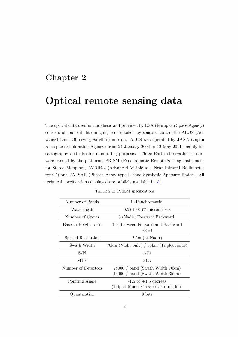
The optical data used in this thesis and provided by ESA (European Space Agency)
consists of four satellite imaging scenes taken by sensors aboard the ALOS (Ad-
vanced Land Observing Satellite) mission. ALOS was operated by JAXA (Japan
Aerospace Exploration Agency) from 24 January 2006 to 12 May 2011, mainly for
cartography and disaster monitoring purposes. Three Earth observation sensors
were carried by the platform: PRISM (Panchromatic Remote-Sensing Instrument
for Stereo Mapping), AVNIR-2 (Advanced Visible and Near Infrared Radiometer
type 2) and PALSAR (Phased Array type L-band Synthetic Aperture Radar). All
technical specifications displayed are publicly available in [5].
Table 2.1: PRISM specifications
Number of Bands 1 (Panchromatic)
Wavelength 0.52 to 0.77 micrometers
Number of Optics 3 (Nadir; Forward; Backward)
Base-to-Height ratio 1.0 (between Forward and Backwardview)
Spatial Resolution 2.5m (at Nadir)
Swath Width 70km (Nadir only) / 35km (Triplet mode)
S/N >70
MTF >0.2
Number of Detectors 28000 / band (Swath Width 70km)14000 / band (Swath Width 35km)
Pointing Angle -1.5 to +1.5 degrees(Triplet Mode, Cross-track direction)
Quantization 8 bits
4
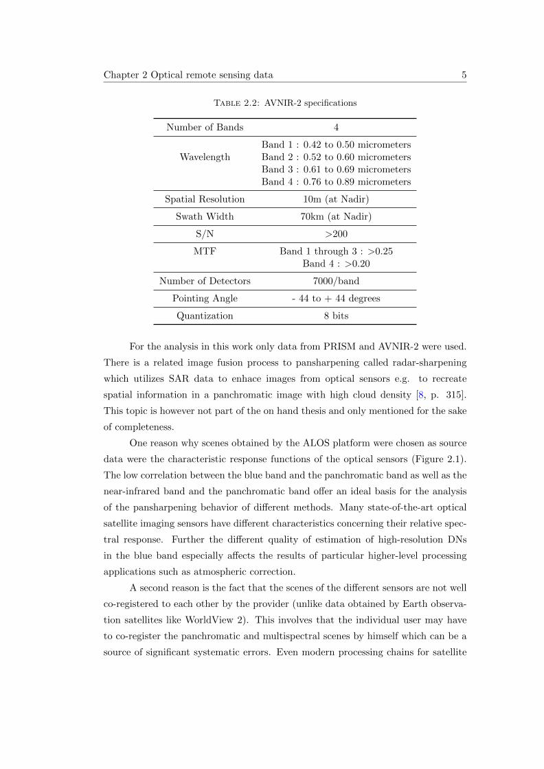
Chapter 2 Optical remote sensing data 5
Table 2.2: AVNIR-2 specifications
Number of Bands 4
Band 1 : 0.42 to 0.50 micrometersWavelength Band 2 : 0.52 to 0.60 micrometers
Band 3 : 0.61 to 0.69 micrometersBand 4 : 0.76 to 0.89 micrometers
Spatial Resolution 10m (at Nadir)
Swath Width 70km (at Nadir)
S/N >200
MTF Band 1 through 3 : >0.25Band 4 : >0.20
Number of Detectors 7000/band
Pointing Angle - 44 to + 44 degrees
Quantization 8 bits
For the analysis in this work only data from PRISM and AVNIR-2 were used.
There is a related image fusion process to pansharpening called radar-sharpening
which utilizes SAR data to enhace images from optical sensors e.g. to recreate
spatial information in a panchromatic image with high cloud density [8, p. 315].
This topic is however not part of the on hand thesis and only mentioned for the sake
of completeness.
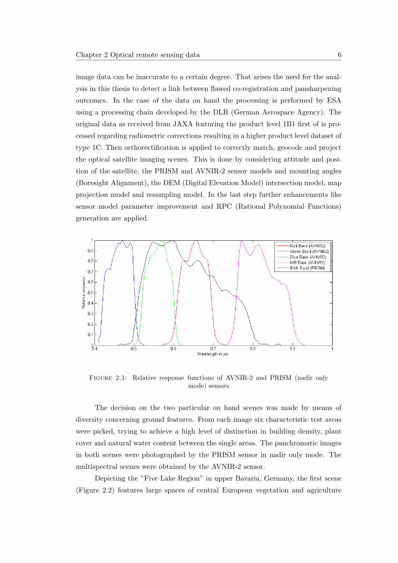
One reason why scenes obtained by the ALOS platform were chosen as source
data were the characteristic response functions of the optical sensors (Figure 2.1).
The low correlation between the blue band and the panchromatic band as well as the
near-infrared band and the panchromatic band offer an ideal basis for the analysis
of the pansharpening behavior of different methods. Many state-of-the-art optical
satellite imaging sensors have different characteristics concerning their relative spec-
tral response. Further the different quality of estimation of high-resolution DNs
in the blue band especially affects the results of particular higher-level processing
applications such as atmospheric correction.
A second reason is the fact that the scenes of the different sensors are not well
co-registered to each other by the provider (unlike data obtained by Earth observa-
tion satellites like WorldView 2). This involves that the individual user may have
to co-register the panchromatic and multispectral scenes by himself which can be a
source of significant systematic errors. Even modern processing chains for satellite
Chapter 2 Optical remote sensing data 6
image data can be inaccurate to a certain degree. That arises the need for the anal-
ysis in this thesis to detect a link between flawed co-registration and pansharpening
outcomes. In the case of the data on hand the processing is performed by ESA
using a processing chain developed by the DLR (German Aerospace Agency). The
original data as received from JAXA featuring the product level 1B1 first of is pro-
cessed regarding radiometric corrections resulting in a higher product level dataset of
type 1C. Then orthorectification is applied to correctly match, geocode and project
the optical satellite imaging scenes. This is done by considering attitude and posi-
tion of the satellite, the PRISM and AVNIR-2 sensor models and mounting angles
(Boresight Alignment), the DEM (Digital Elevation Model) intersection model, map
projection model and resampling model. In the last step further enhancements like
sensor model parameter improvement and RPC (Rational Polynomial Functions)
generation are applied.
Figure 2.1: Relative response functions of AVNIR-2 and PRISM (nadir onlymode) sensors
The decision on the two particular on hand scenes was made by means of
diversity concerning ground features. From each image six characteristic test areas
were picked, trying to achieve a high level of distinction in building density, plant
cover and natural water content between the single areas. The panchromatic images
in both scenes were photographed by the PRISM sensor in nadir only mode. The
multispectral scenes were obtained by the AVNIR-2 sensor.
Depicting the ”Five Lake Region” in upper Bavaria, Germany, the first scene
(Figure 2.2) features large spaces of central European vegetation and agriculture
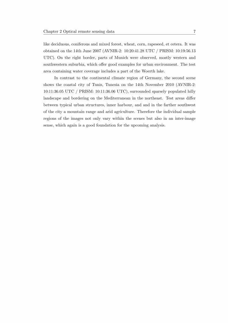
Chapter 2 Optical remote sensing data 7
like deciduous, coniferous and mixed forest, wheat, corn, rapeseed, et cetera. It was
obtained on the 14th June 2007 (AVNIR-2: 10:20:41.28 UTC / PRISM: 10:19:56.13
UTC). On the right border, parts of Munich were observed, mostly western and
southwestern suburbia, which offer good examples for urban environment. The test
area containing water coverage includes a part of the Woerth lake.
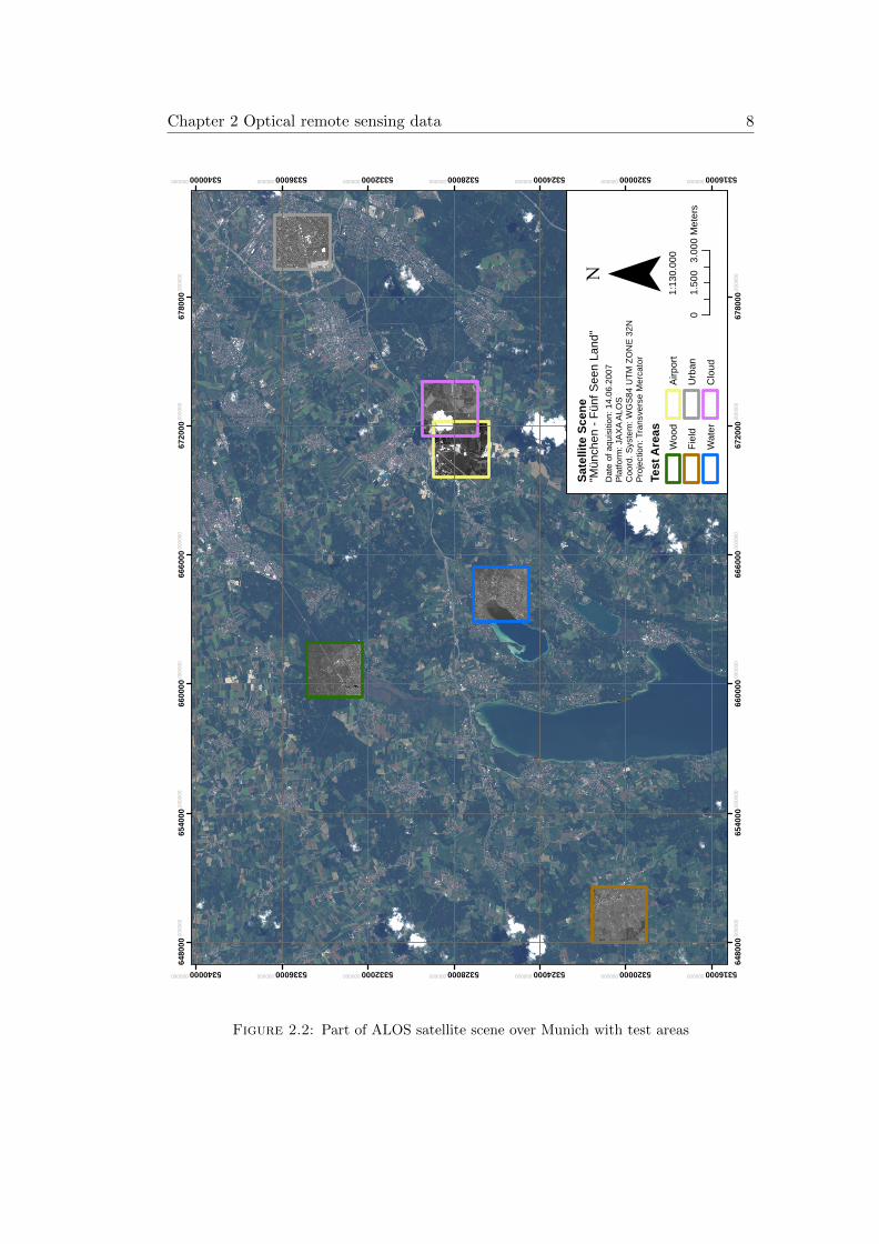
In contrast to the continental climate region of Germany, the second scene
shows the coastal city of Tunis, Tunesia on the 14th November 2010 (AVNIR-2:
10:11:36.05 UTC / PRISM: 10:11:36.06 UTC), surrounded sparsely populated hilly
landscape and bordering on the Mediterranean in the northeast. Test areas differ
between typical urban structures, inner harbour, and and in the farther southwest
of the city a mountain range and arid agriculture. Therefore the individual sample
regions of the images not only vary within the scenes but also in an inter-image
sense, which again is a good foundation for the upcoming analysis.
Chapter 2 Optical remote sensing data 8
6480
00,0
0000
0
6480
00,0
0000
0
6540
00,0
0000
0
6540
00,0
0000
0
6600
00,0
0000
0
6600
00,0
0000
0
6660
00,0
0000
0
6660
00,0
0000
0
6720
00,0
0000
0
6720
00,0
0000
0
6780
00,0
0000
0
6780
00,0
0000
0
5316000,000000
5316000,000000
5320000,000000
5320000,000000
5324000,000000
5324000,000000
5328000,000000
5328000,000000
5332000,000000
5332000,000000
5336000,000000
5336000,000000
5340000,000000
5340000,000000
Test
Are
as
Woo
d
Fie
ld
Wat
er
Airp
ort
Urb
an
Clo
ud
1:13
0.00
0
Sat
ellit
e S
cen
e"M
ünch
en -
Fün
f See
n La
nd"
Dat
e of
aqu
isiti
on: 1
4.06
.200
7P
latfo
rm: J
AX
A A
LOS
Coo
rd. S
yste
m: W
GS
84 U
TM
ZO
NE
32N
Pro
ject
ion:
Tra
nsve
rse
Mer
cato
r
03.
000
1.50
0M
eter
s
Figure 2.2: Part of ALOS satellite scene over Munich with test areas
Chapter 2 Optical remote sensing data 9
588000,000000
588000,000000
594000,000000
594000,000000
600000,000000
600000,000000
606000,000000
606000,000000
612000,000000
612000,000000
4044
000,0
0000
0
4044
000,0
0000
0
4048
000,0
0000
0
4048
000,0
0000
0
4052
000,0
0000
0
4052
000,0
0000
0
4056
000,0
0000
0
4056
000,0
0000
0
4060
000,0
0000
0
4060
000,0
0000
0
4064
000,0
0000
0
4064
000,0
0000
0
4068
000,0
0000
0
4068
000,0
0000
0
4072
000,0
0000
0
4072
000,0
0000
0
4076
000,0
0000
0
4076
000,0
0000
0
4080
000,0
0000
0
4080
000,0
0000
0
4084
000,0
0000
0
4084
000,0
0000
0
4088
000,0
0000
0
4088
000,0
0000
0
Test Areas
Water
Urban
Sand
Airport
Mountains
Vegetation
0 4.0002.000 Meters
1:175.000
Satellite Scene"Tunis"Date of aquisition: 14.11.2010Platform: JAXA ALOSCoord. System: WGS84 UTM ZONE 32NProjection: Transverse Mercator
Figure 2.3: Part of ALOS satellite scene over Tunis with test areas
Chapter 3
Pansharpening methods
In the course of this work two specific pansharpening methods were employed to
produce high-resolution images. The GIHS is an advanced variant of the basic
Intensity-Hue-Saturation image fusion method. The SCFF is a rather novel approach
to pansharpening with its attention turned on maintaining complete and correct
spectral information in the resulting data. These methods were intentionally chosen
for their elementary differences in how they solve the image fusion problem. In the
following sections the characteristics of each will be described in detail.
3.1 GIHS
The first approach used in this thesis is the IHS technique which has been used in
the remote sensing context since 1987 [3] and is one of the most common methods
in commercial software solutions. It queues in the category of component substitu-
ton procedures and stands out due to its fairly straightforward functionality. The
pixelwise process can be expressed by the following equations, as described in [10].
1. The multi-spectral image is upsampled to the resolution of the panchromatic
image. In the course of this thesis, upsampling at this step is done using
nearest-neighbour interpolation to avoid a pre-pansharpening spectral distor-
tion effect.
2. Then a transformation in the IHS colorspace is conducted.I
v1
v2
=
13
13
13
−√
26 −
√2
62√
26
1√2− 1√
20
R
G
B
(3.1)
10
Chapter 3 Pansharpening methods 11
where I represents the intensity part of the pixel and v1, v2 the corresponding
hue and saturation values.
3. The intensity part of the IHS image is substituted by the PAN image. The
reverse transformation results in a high-resolution RGB image.RHR
GHR
BHR
=
1 − 1√
21√2
1 − 1√2− 1√
2
1√
2 0
PAN
v1
v2
(3.2)
As the whole calculation can be rewritten into a single, pixelwise addition (3.3),
one advantage of this method lies in its high computational efficiency. Further the
spatial information of the PAN image is completely induced into the multi-band
image, which results in a high geometric accuracy.
On the other hand IHS image fusion is very susceptible to a main problem
of pansharpening. In order to generate spectrally consistent high-resolution RGB
data, an appropriate correlation between the relative response functions of the sin-
gle bands of the multi-spectral sensor and the panchromatic band is necessary. In
practice such a congruency is seldom achieved. This results in a color shift of the
pansharpened image and accordingly in a falsification of the pristine spectral infor-
mation. Depending on the degree of band correlation the color shift is stronger or
less intense and thus more or less optically recognizable. Another inherent issue is
that the transformation as it is displayed in equation (3.1) and (3.2) can only be
applied to three channels, by default the RGB combination of a multi-band sensor.
As mentioned earlier, the IHS transformation can be expressed as described
in [10], [11]: RHR
GHR
BHR
=
1 − 1√
21√2
1 − 1√2− 1√
2
1√
2 0
I + (PAN − I)
v1
v2
=
1 − 1√
21√2
1 − 1√2− 1√
2
1√
2 0
I + δ
v1
v2
=
R+ δ
G+ δ
B + δ
(3.3)
where
δ = PAN − I. (3.4)
This conversion not only enhances the computation speed of the whole procedure,
but also enables to get rid of the afore described three channel constraint. The last
Chapter 3 Pansharpening methods 12
transformation term as proposed in [10] is extended to the form:RHR
GHR
BHR
NIRHR
=
R+ δ4
G+ δ4
B + δ4
NIR+ δ4
(3.5)
where
δ4 = PAN − (R+G+B +NIR)/4. (3.6)
with
R,G,B,NIRdenoting the red, green, blue and near infrared band of the AVNIR-2 sensor.
The per-pixel intensity values of the panchromatic image are equally distributed into
the individual multispectral bands. In equation 3.5 the full multispectral bandwidth
of the ALOS satellite optical image data is used for the pansharpening process. This
results in a smaller color shift especially in regions of dense vegetation, which feature
a high spectral response in the near infrared range of wavelengths.
The GIHS pansharpening method was implemented in Matlab as follows:
intensityMatrix = sum((MS / bands), 3);
IMD = cat(3, PAN - intensityMatrix , ...
PAN - intensityMatrix , ...
PAN - intensityMatrix , ...
PAN - intensityMatrix );
IHS = MS + IMD;
3.2 SCFF
The second approach used in this thesis is the SCFF (Spectrally Consistent Fusion
Framework) as proposed by H. Aanæs et al. [1]. It represends a rather unique and
novel method which ”is model based, and the fused images obtained spectrally are
consistent by design”[1, p. 1336].
Spectral consistency is achieved by deriving a ratio vector from the sensors’
response function, which describes fracture values of the single multispectral bands
Chapter 3 Pansharpening methods 13
contained in the panchromatic pixels:
~R =
α(1,PAN)
α(2,PAN)
...
α(n,PAN)
(3.7)
where
α(i,PAN) =〈F i, FPAN 〉√
〈F i, F i〉〈FPAN , FPAN 〉(3.8)
with
i ∈ 1 . . . n(Total number of multispectral bands)
The inner product 〈F i, FPAN 〉 represents the integral over the spectral response
functions of a certain range of wavelengths Ω of the corresponding multispectral
band and the panchromatic sensor:
〈F i, FPAN 〉 =
∫Ω
F i(ω)FPAN (ω)dω (3.9)
This, as seen in the equations above, opens up the possibility to address every band of
the multispectral sensor to generate a fused image. For the proper calculation of the
ratio vector a previous knowledge of the exact relative spectral response functions of
the applied sensor must be postulated. In the course of the on hand thesis ~R for the
ALOS AVNIR-2 sensor with respect to the panchromatic channel of ALOS PRISM
(nadir only mode) was calculated as:
~RAV NIR2 =
αBlue
αGreen
αRed
αNIR
=
0.015
0.688
0.606
0.174
In the next step for each pixel i in the multispectral image, sixteen corresponding
multispectral pixels i, j, j ∈ [1, . . . , 16] containing the spatial information of the
panchromatic image are generated by weighing the panchromatic intensity data with
the before determined ratio vector. The number of exactly sixteen corresponding
pixels for each multispectral pixel i is derived from the 1 : 16 ratio of the 10m × 10
m ground resolution of the AVNIR-2 sensor and the 2.5 m × 2.5 m ground resolution
Chapter 3 Pansharpening methods 14
of PRISM. ∆IBlueij
∆IGreenij
∆IRedij
∆INIRij
=
αBlue
αGreen
αRed
αNIR
(PHRij − Pµi ) (3.10)
with
Pµi =
16∑j=1
PHRij
16.
One important aspect of equation 3.10 is the subtraction of Pµi , which denotes the
mean of the sixteen pixels corresponding to the low resolution pixel i. It results in a
relative description of the spatial frequency of the relevant high-resolution four-by-
four pixel region.
Image fusion is then conducted by infusing the spatial information pixel by
pixel into the multispectral image through addition:BHRij
GHRij
RHRij
NIRHRij
=
BLRi
GLRi
RLRi
NIRLRi
+
∆IBlueij
∆IGreenij
∆IRedij
∆INIRij
(3.11)
(a) (b) (c)
(d) (e) (f)
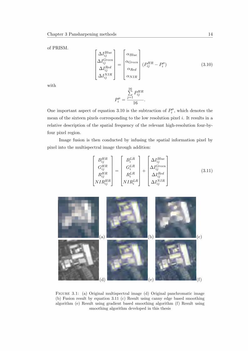
Figure 3.1: (a) Original multispectral image (d) Original panchromatic image(b) Fusion result by equation 3.11 (c) Result using canny edge based smoothingalgorithm (e) Result using gradient based smoothing algorithm (f) Result using
smoothing algorithm developed in this thesis
Chapter 3 Pansharpening methods 15
As proofed in [1] the resulting high-resolution images offer spectral consistency
but also suffer from a rather blocky appearence (compare Figure 3.1b). To further
enhance the visual appearance while sustaining spectral resolution, the authors of
[1] introduce different smoothing algorithms by weighing singular pixels by edge and
gradient extraction of the spatial data (Figure 3.1c & d).
The results of this further processing where decided to be insufficient for the
thesis at hand, as they tend to blur the final image data while weirdly emphasizing
structural edges.
Therefore a new algorithm to reduce the induced block artifacts was devel-
oped, aiming to maintain spectral consistent band intensities and achieving best
possible spatial resolution alike. To accomplish this, high resolution result images
from both presented fusion methods were used. The spectrally consistant (though
blocky) pansharpened image and the GIHS image are processed by a sliding-window
operation using a three-by-three window. In both cases the mean of each respective
window is calculated and the GIHS mean value is substracted from the SCFF mean
value. The difference is then added to the GIHS pixel corresponding to the center
pixel of the actual window position. Thereby an enhancement is applied to every
pixel of the GIHS image, derived from the SCFF image. This process induces a
very high spatial accuracy compared to the above mentioned smoothing techniques,
while improving the intensity of each band of the GIHS image to near spectrally
consistent quality (as shown in Figure 3.1f). The pixelwise approach, which needs
to be employed for each band separately, can be mathematically represented as:
PHR′
ij = PGIHSij + µij (3.12)
with
µij =
∑k∈Wij
PSCFFk
9−
∑k∈Wij
PGIHSk
9(3.13)
Wij denotes the eight-neighbourhood with respect to the high-resolution image over
the centerpixel Pij . The application of a sliding window entails that the border-pixels
of the used images can not be considered in this step. The prior SCFF images as
well as the representative images of the proposed canny and gradient based weighting
algorithms [1] were generated in Matlab using the code provided on the main authors
website [2]. The improved smoothing algorithm was developed in MatLab as well:
wait = waitbar(0, ’Smoothing Image ...’);
blockCalc = @(x, y) mean(mean(x)) - mean(mean(y));
Chapter 3 Pansharpening methods 16
for row = 1:size(RGBconsistent , 1)
for col = 1:size(RGBconsistent , 2)
if row == 1 && col == 1
PANSHARP(row , col , :) = IHS(row , col , :) + ...
blockCalc(RGBconsistent(row:row+1, col:col+1, :), ...
IHS(row:row+1, col:col+1, :));
elseif row == 1 && col == size(RGBconsistent , 2)
PANSHARP(row , col , :) = IHS(row , col , :) + ...
blockCalc(RGBconsistent(row:row+1, col -1:col , :), ...
IHS(row:row+1, col -1:col , :));
elseif row == size(RGBconsistent , 1) && col == 1
PANSHARP(row , col , :) = IHS(row , col , :) + ...
blockCalc(RGBconsistent(row -1:row , col:col+1, :), ...
IHS(row -1:row , col:col+1, :));
elseif row == size(RGBconsistent , 1) && col == size(RGBconsistent , 2)
PANSHARP(row , col , :) = IHS(row , col , :) + ...
blockCalc(RGBconsistent(row -1:row , col -1:col , :), ...
IHS(row -1:row , col -1:col , :));
elseif row == 1
PANSHARP(row , col , :) = IHS(row , col , :) + ...
blockCalc(RGBconsistent(row:row+1, col -1:col+1, :), ...
IHS(row:row+1, col -1: col+1, :));
elseif col == 1
PANSHARP(row , col , :) = IHS(row , col , :) + ...
blockCalc(RGBconsistent(row -1:row+1, col:col+1, :), ...
IHS(row -1:row+1, col:col+1, :));
elseif col == size(RGBconsistent , 2)
PANSHARP(row , col , :) = IHS(row , col , :) + ...
blockCalc(RGBconsistent(row -1:row+1, col -1:col , :), ...
IHS(row -1:row+1, col -1:col , :));
elseif row == size(RGBconsistent , 1)
PANSHARP(row , col , :) = IHS(row , col , :) + ...
blockCalc(RGBconsistent(row -1:row , col -1:col+1, :), ...
IHS(row -1:row , col -1: col+1, :));
else
PANSHARP(row , col , :) = IHS(row , col , :) + ...
blockCalc(RGBconsistent(row -1:row+1, col -1: col+1, :),...
IHS(row -1:row+1, col -1:col+1, :));
end
end
waitbar(row/size(RGBconsistent , 1), wait);
end
Chapter 4
Experiments
4.1 Quality metrics
In the of the evaluation of pansharpened images two different factors of quality
must be considered. On one hand it must be measured how much of the geometric
information contained in the high-resolution panchromatic image was successfully
induced into the fused image, on the other hand the degree of accuracy concerning
the reconstruction of the original spectral characteristics of a optical remote sensing
scene has to be described. In both cases a first, reliable judgement can be made by
human vision to identify gross errors. But with deviations growing smaller, especially
in the case of color shifts, the human eye fails to recognize differences.
Therefore many efforts has be made to develop dependable quality metrics to
detect even small changes in the image structure. For the analysis at hand four com-
monly used indicators were used to review the results of the introduced pansharp-
ening methods. For the evaluation of spatial similarity the correlation coefficient[4,
p. 1596] is used, which resembles a widely applied statistical metric concerning
interrelation between two different parameters. Addressing the quantitation of spec-
tral consistency quality is expressed by SAM (Spectral Angle Mapper)[4, p. 1597],
which is used in many different remote sensing applications. Approaching the more
special case of pansharpening in particular, two further indices were chosen, aiming
to provide a simple, combined quality metrics concerning image fusion results. By
name these are ERGAS (Erreur Relative Globale Adimensionelle de Synthese) as
proposed in [13] and Q-Index introcuded in [14].
In order to detect geometric similarity, high-frequency spatial information has
to be extracted from the images to be compared. Therefore every single band of
the pansharpened image (PS) and the reference image (R) are convoluted with a
17
Chapter 4 Experiments 18
high-pass filter shown in equation 4.1. Border-pixels are treated by means of border
replication.
HPF =
−1 −1 −1
−1 8 −1
−1 −1 −1
(4.1)
Then the correlation coefficient for each pair of corresponding band of fused
and high-resolution reference image is calculated.
CC =σR,PS
σR ∗ σPS(4.2)
with
σR = unbiased standard deviation of reference image (HR PAN)
σPS = unbiased standard deviation of pansharpened image
σR,PS = unbiased covariance between reference and pansharpened image
By determining the mean of the CCs of the single bands an overall validation
is given ranging from -1 (negative correlation) to 1 (positive correlation) as the best
possible outcome.
SAM denotes the angular difference between two spectra. The spectral charac-
teristics of a pixel are given by the individual combination of DNs (digital numbers)
considering all bands. This combination can be expressed as a vector. By generating
spectral vectors of a corresponding pixel pair in the reference and the fused image,
its similarity can be expressed as the arccosine of the dot product between the two
vectors [4][15]:
SAM(R,PS) = arccos
(〈R,PS〉
‖ ~R ‖ · ‖ ~PS ‖
)(4.3)
which can be written as [15]
SAM(R,PS) = arccos
n∑i=1
RiPSi√n∑i=1
R2i
√n∑i=1
PS2i
(4.4)
where
Chapter 4 Experiments 19
n = total number of bands.
Again the indicator is applied to every corresponding pixel pair and the mean
for the whole scene is calculated to give an overall measure for spectral similarity.
In this work SAM is given in degrees with lower angels describing better results.
With ERGAS Wald proposed a statistical overall value for judging image fusion
quality, which is derived of the commonly used RMSE (Root Mean Square Error)
but provides a higher robustness with respect to calibration and changes of units
[13]. First the RMSE between the reference image and the pansharpened image has
to be determined [4]:
RMSE =
√√√√√ M∑i=1
N∑j=1
(Ri,j − PSi,j)2
M ×N(4.5)
whereM ×N = size of the images.
Ri,j = Pixel in row i, column j in reference image.
PSi,j = Pixel in row i, column j in fused image.
This is conducted bandwise, giving n RMSE values for n spectral channels. Subse-
quently ERGAS is obtained by the following equation [13]:
ERGAS = 100h
l
√√√√ 1
n
n∑i=1
RMSE2i
µ2i
(4.6)
whereh = ground pixel resolution of HR image
l = ground pixel resolution of LR image
µi = mean of intensity values in band i
n = total number of bands.
Wald stated in [13, p. 102] that based on experimental observations a threshold
of 3 is a representative assessment value, with results featuring lower values being
of good overall quality.
As a last quality metric the Q-index introduced by Wang and Bovik was cho-
sen. ”Instead of using traditinoal error summation methods, the proposed index is
designed by modeling any image distortion as a combination of three factors: loss
Chapter 4 Experiments 20
of correlation, luminance distortion and contrast distortion”[14, p. 81]. Therefore it
gives an opportunity to review the image fusion results of the on hand thesis with a
different approach. The Q-index is formulated as (again applied seperately to every
single band of the sensor data):
Q =4 · σR,PS · µR · µPS
(σ2R + σ2
PS)[(µR)2 + (µPS)2](4.7)
withµR = pixel mean value of reference image
µPS = pixel mean value of pansharpened image
Further equation 4.7 can be rearranged [14, p. 81] to depict the three factors
influencing the Q-index:
Q =σR,PSσRσPS
· 2µRµPS(µR)2 + (µPS)2
· 2σRσPSσ2R + σ2
PS
(4.8)
Here the first component is the correlation coefficient between the reference and
the fused band. The second part describes the difference of the mean luminance
between R and PS and the third component measures the similiarity of contrast. As
mentioned earlier the calculation of the Q-index is conducted for every corresponding
band. A mean Q-index is then generated to give an overall value for general fusion
quality. It can adopt values in the dynamic range of [0, 1] with one being the best
value, only achieved if the two compared images are identical (this also applies for
all other quality metrics).
4.2 Quality assessment
As mentioned before four optical satellite imaging scenes were chosen as the basis
of the analysis. From each six test areas were picked to cover a large variety of
ground features. The areas are quadratic, with a size of 1024 by 1024 pixels for the
panchromatic images and 256 by 256 pixels for the lower resoluton multispectral
images. In both cases this equals a ground edge length of of 2560 meters.
Regarding the evaluation conducted in this thesis one important point is men-
tioned. One inherent problem of the assessment of pansharpening methods is the
lack of a multispectral high-resolution reference images obtained by the same sen-
sor (as on one part this is technically not possible, on the other it would make the
whole pansharpening process unnecessary)[12, p. 696]. Therefore the pansharpened
Chapter 4 Experiments 21
images were down-sampled by cubic interpolation to the resolution of the original
multispectral image. Then the pixel values of the lower resolution multispectral im-
age can be seen as mixed pixel values of a theoretical high-resolution multispectral
image with the same spectral characteristics. A completely spectrally consistent
fused image would thus, regarding the resolution ratio of the scenes used in this
thesis, satisfy the criterion[1, p. 1338]:BMSi
GMSi
RMSi
NIRMSi
=1
16
16∑j=1
BPSij
GPSij
RPSij
NIRPSij
(4.9)
Concerning the analysis of the results of spatial properties, the pansharpened
images were compared with the original high-resolution panchromatic scene, as the
geometric data available in the resulting images dervies from that source. Tables 4.1
and 4.2 show the complete list of the results.
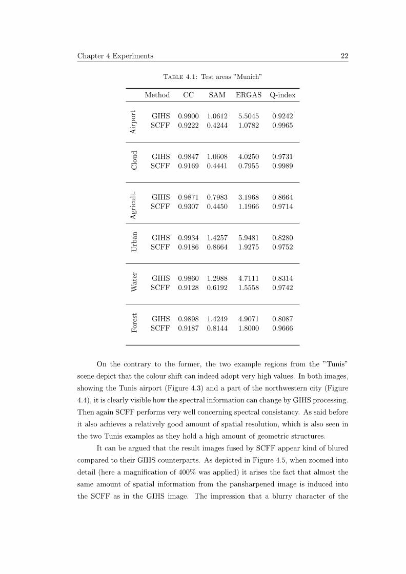
The results in tables 4.1 and 4.2 show that the overall performance of the
two chosen methods is constantly is very high regarding spectral and geometric
consistency. Especially the SCFF features very good quality. Looking at the quality
metrics GIHS only excels concerning the spatial correlation coefficient, which is due
to the fundamental principles of operation of the two pansharpening techniques.
On the other hand, concerning geometric quality SCFF only suffers from a slightly
greater loss of spatial information. The four examples shown in this chapter depict
the test areas in which the difference in results of the two pansharpening methods
are greatest and therefore most comprehensible by human vision.
Looking at the two test areas from the ”Munich” scene, it is evident that
the spectral consistency achieved by GIHS is very dependent on the reflectance
value and spectral combination of the multispectral channels. Although the two
regions feature a high density of vegetation (Figure 4.1), which usually have a high
reflectance in the near-infrared band, and big patches of water (Figure 4.2) a colour
shift is merely visible by the human eye considering true color representation (which
also applies to the other ”Munich” test areas). This shows that for the evaluation
of pansharpening results quality measures are needed to qualify and quantify the
decisions which method delivers the best outcomes which may depend on the specific
application. Further the two examples illustrate that it is not advisable to trivialize
the performance of one particular image fusion method but to link it to the properties
of the source data.
Chapter 4 Experiments 22
Table 4.1: Test areas ”Munich”
Method CC SAM ERGAS Q-index
Air
port GIHS 0.9900 1.0612 5.5045 0.9242
SCFF 0.9222 0.4244 1.0782 0.9965C
lou
d
GIHS 0.9847 1.0608 4.0250 0.9731SCFF 0.9169 0.4441 0.7955 0.9989
Agri
cult
.
GIHS 0.9871 0.7983 3.1968 0.8664SCFF 0.9307 0.4450 1.1966 0.9714
Urb
an GIHS 0.9934 1.4257 5.9481 0.8280SCFF 0.9186 0.8664 1.9275 0.9752
Wat
er GIHS 0.9860 1.2988 4.7111 0.8314SCFF 0.9128 0.6192 1.5558 0.9742
For
est
GIHS 0.9898 1.4249 4.9071 0.8087SCFF 0.9187 0.8144 1.8000 0.9666
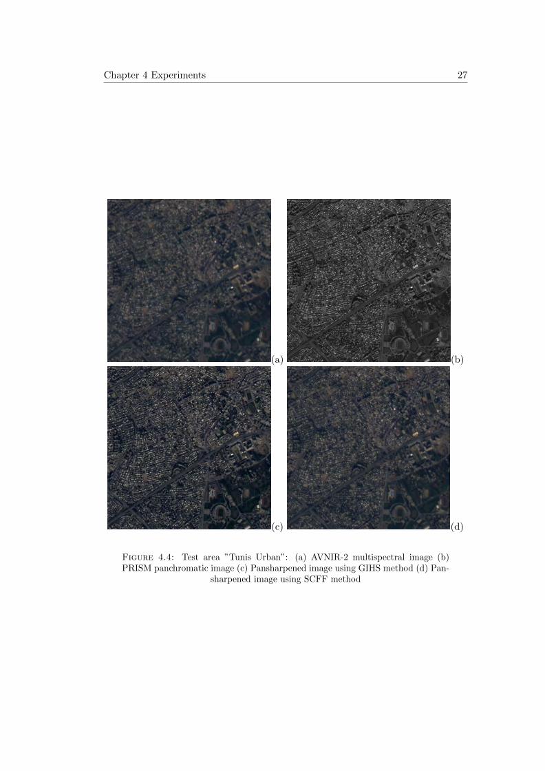
On the contrary to the former, the two example regions from the ”Tunis”
scene depict that the colour shift can indeed adopt very high values. In both images,
showing the Tunis airport (Figure 4.3) and a part of the northwestern city (Figure
4.4), it is clearly visible how the spectral information can change by GIHS processing.
Then again SCFF performs very well concerning spectral consistancy. As said before
it also achieves a relatively good amount of spatial resolution, which is also seen in
the two Tunis examples as they hold a high amount of geometric structures.
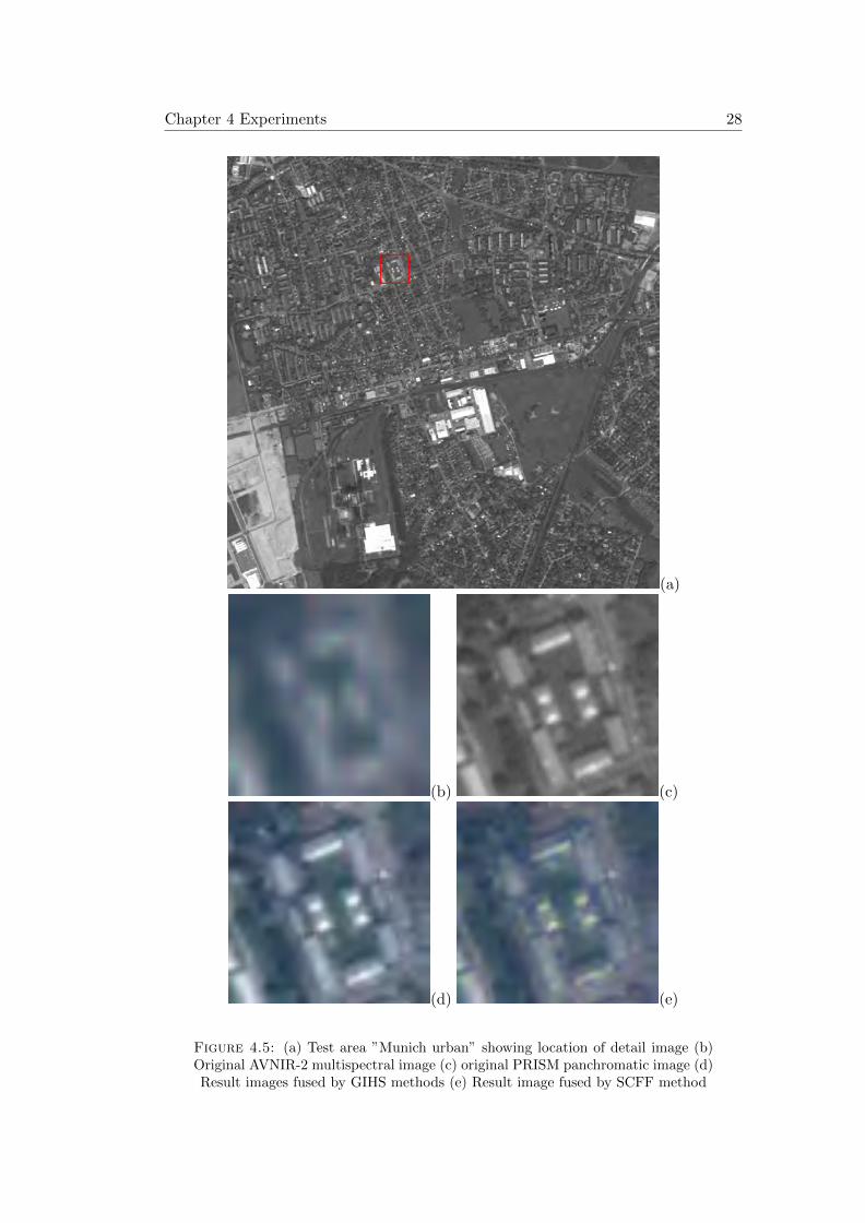
It can be argued that the result images fused by SCFF appear kind of blured
compared to their GIHS counterparts. As depicted in Figure 4.5, when zoomed into
detail (here a magnification of 400% was applied) it arises the fact that almost the
same amount of spatial information from the pansharpened image is induced into
the SCFF as in the GIHS image. The impression that a blurry character of the
Chapter 4 Experiments 23
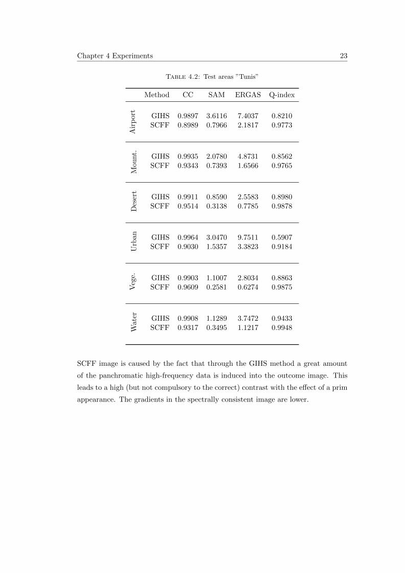
Table 4.2: Test areas ”Tunis”
Method CC SAM ERGAS Q-index
Air
port GIHS 0.9897 3.6116 7.4037 0.8210
SCFF 0.8989 0.7966 2.1817 0.9773M
ou
nt. GIHS 0.9935 2.0780 4.8731 0.8562
SCFF 0.9343 0.7393 1.6566 0.9765
Des
ert
GIHS 0.9911 0.8590 2.5583 0.8980SCFF 0.9514 0.3138 0.7785 0.9878
Urb
an GIHS 0.9964 3.0470 9.7511 0.5907SCFF 0.9030 1.5357 3.3823 0.9184
Veg
e. GIHS 0.9903 1.1007 2.8034 0.8863SCFF 0.9609 0.2581 0.6274 0.9875
Wat
er GIHS 0.9908 1.1289 3.7472 0.9433SCFF 0.9317 0.3495 1.1217 0.9948
SCFF image is caused by the fact that through the GIHS method a great amount
of the panchromatic high-frequency data is induced into the outcome image. This
leads to a high (but not compulsory to the correct) contrast with the effect of a prim
appearance. The gradients in the spectrally consistent image are lower.
Chapter 4 Experiments 24
(a) (b)
(c) (d)
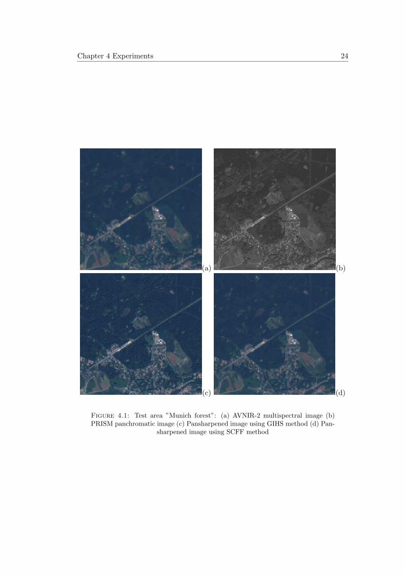
Figure 4.1: Test area ”Munich forest”: (a) AVNIR-2 multispectral image (b)PRISM panchromatic image (c) Pansharpened image using GIHS method (d) Pan-
sharpened image using SCFF method
Chapter 4 Experiments 25
(a) (b)
(c) (d)
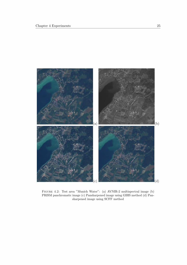
Figure 4.2: Test area ”Munich Water”: (a) AVNIR-2 multispectral image (b)PRISM panchromatic image (c) Pansharpened image using GIHS method (d) Pan-
sharpened image using SCFF method
Chapter 4 Experiments 26
(a) (b)
(c) (d)
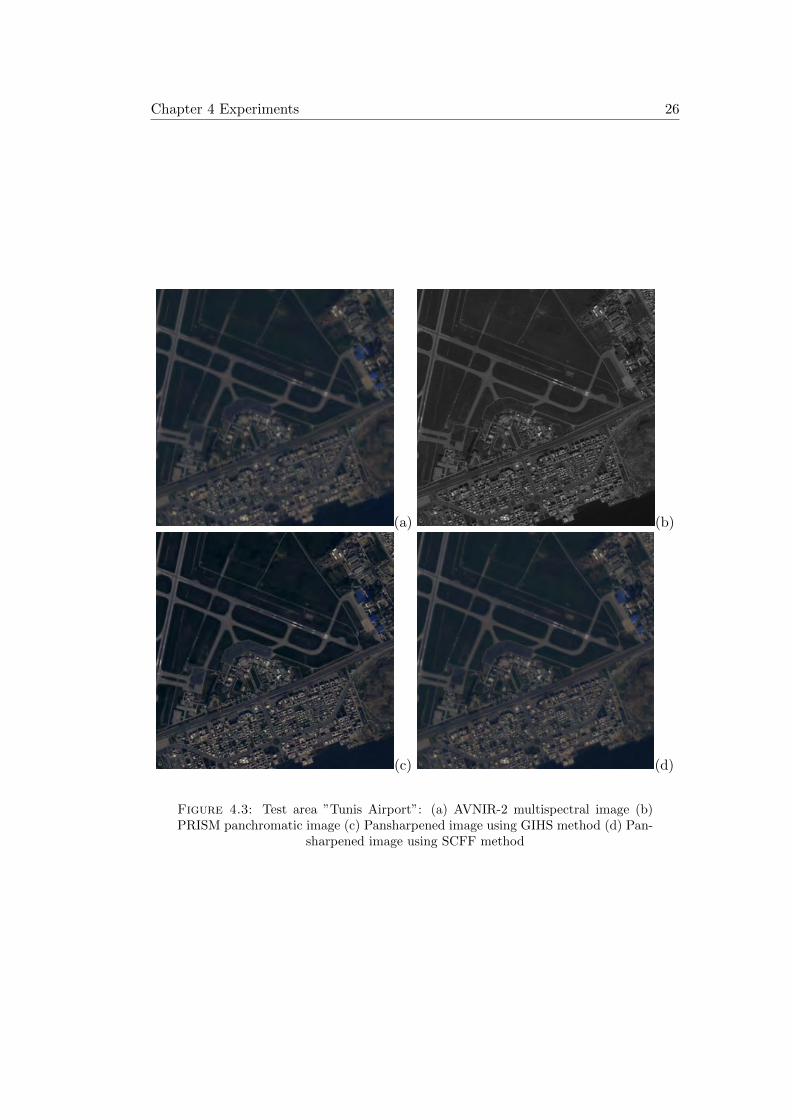
Figure 4.3: Test area ”Tunis Airport”: (a) AVNIR-2 multispectral image (b)PRISM panchromatic image (c) Pansharpened image using GIHS method (d) Pan-
sharpened image using SCFF method
Chapter 4 Experiments 27
(a) (b)
(c) (d)
Figure 4.4: Test area ”Tunis Urban”: (a) AVNIR-2 multispectral image (b)PRISM panchromatic image (c) Pansharpened image using GIHS method (d) Pan-
sharpened image using SCFF method
Chapter 4 Experiments 28
(a)
(b) (c)
(d) (e)
Figure 4.5: (a) Test area ”Munich urban” showing location of detail image (b)Original AVNIR-2 multispectral image (c) original PRISM panchromatic image (d)Result images fused by GIHS methods (e) Result image fused by SCFF method
Chapter 4 Experiments 29
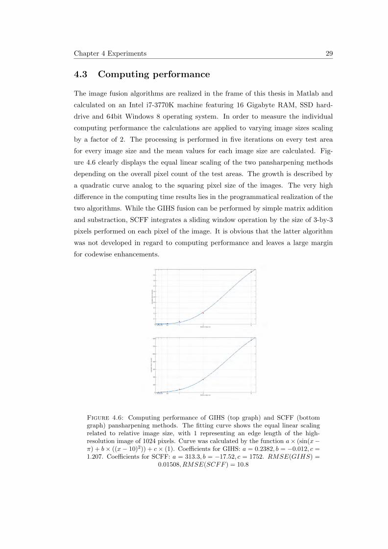
4.3 Computing performance
The image fusion algorithms are realized in the frame of this thesis in Matlab and
calculated on an Intel i7-3770K machine featuring 16 Gigabyte RAM, SSD hard-
drive and 64bit Windows 8 operating system. In order to measure the individual
computing performance the calculations are applied to varying image sizes scaling
by a factor of 2. The processing is performed in five iterations on every test area
for every image size and the mean values for each image size are calculated. Fig-
ure 4.6 clearly displays the equal linear scaling of the two pansharpening methods
depending on the overall pixel count of the test areas. The growth is described by
a quadratic curve analog to the squaring pixel size of the images. The very high
difference in the computing time results lies in the programmatical realization of the
two algorithms. While the GIHS fusion can be performed by simple matrix addition
and substraction, SCFF integrates a sliding window operation by the size of 3-by-3
pixels performed on each pixel of the image. It is obvious that the latter algorithm
was not developed in regard to computing performance and leaves a large margin
for codewise enhancements.
Figure 4.6: Computing performance of GIHS (top graph) and SCFF (bottomgraph) pansharpening methods. The fitting curve shows the equal linear scalingrelated to relative image size, with 1 representing an edge length of the high-resolution image of 1024 pixels. Curve was calculated by the function a× (sin(x−π) + b× ((x− 10)2)) + c× (1). Coefficients for GIHS: a = 0.2382, b = −0.012, c =1.207. Coefficients for SCFF: a = 313.3, b = −17.52, c = 1752. RMSE(GIHS) =
0.01508, RMSE(SCFF ) = 10.8
Chapter 5
Discussion
5.1 The influence of co-registration errors on pansharp-
ening methods
In the last chapter the performance of the two presented pansharpening methods
was shown, revealing that SCFF constantly provides better results from a spectral
point of view. As it also gives only slightly worse results as GIHS from a spatial
point of view it allover can be seen as the more efficient algorithm.
In this chapter the analysis and discussion of how both fusion methods behave
if the pansharpening process is conducted with source data that holds small and big
co-registration errors. By manually measuring the geometric shift in both scenes
the co-registration error was determined to average about 276 meters (regarding
the unmatched level 1B product). The fact that corresponding multispectral and
panchromatic images possessing an error to that extent can be seen as two completely
different images manifests in Figures 5.1 and 5.2, showing that an evaluation of the
pansharpening behavior cannot be conducted on the basis of this data.
This is further reinforced by the multispectral and panchromatic images both
being shifted from the location of a reference image without (major) co-registration
errors. Therefore a series of test areas containing increasing errors in the subpixel
range of both sensors was synthetically generated by, starting from a quasi error-free
image pair, shifting the multispectral image by the amount of 1 m in the x- and y-
directions up to a displacement of 276 meters, matching the co-registration error of
the original source data and providing a sufficient length of measurement to predict
the pansharpening behaviour corning even greater co-registration errors. This was
achieved by a stepwise manipulation of the coordinates of the correctly geocoded
multispectral image and then resampling the multispectral image to its new location
30
Chapter 5 Discussion 31
(a) (b)
(c) (d)
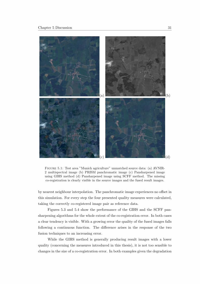
Figure 5.1: Test area ”Munich agriculture” unmatched source data: (a) AVNIR-2 multispectral image (b) PRISM panchromatic image (c) Pansharpened imageusing GIHS method (d) Pansharpened image using SCFF method. The missingco-registration is clearly visible in the source images and the fused result images.
by nearest neighbour interpolation. The panchromatic image experiences no offset in
this simulation. For every step the four presented quality measures were calculated,
taking the correctly co-registered image pair as reference data.
Figures 5.3 and 5.4 show the performance of the GIHS and the SCFF pan-
sharpening algorithms for the whole extent of the co-registration error. In both cases
a clear tendency is visible. With a growing error the quality of the fused images falls
following a continuous function. The difference arises in the response of the two
fusion techniques to an increasing error.
While the GIHS method is generally producing result images with a lower
quality (concerning the measures introduced in this thesis), it is not too sensible to
changes in the size of a co-registration error. In both examples given the degradation
Chapter 5 Discussion 32
(a) (b)
(c) (d)
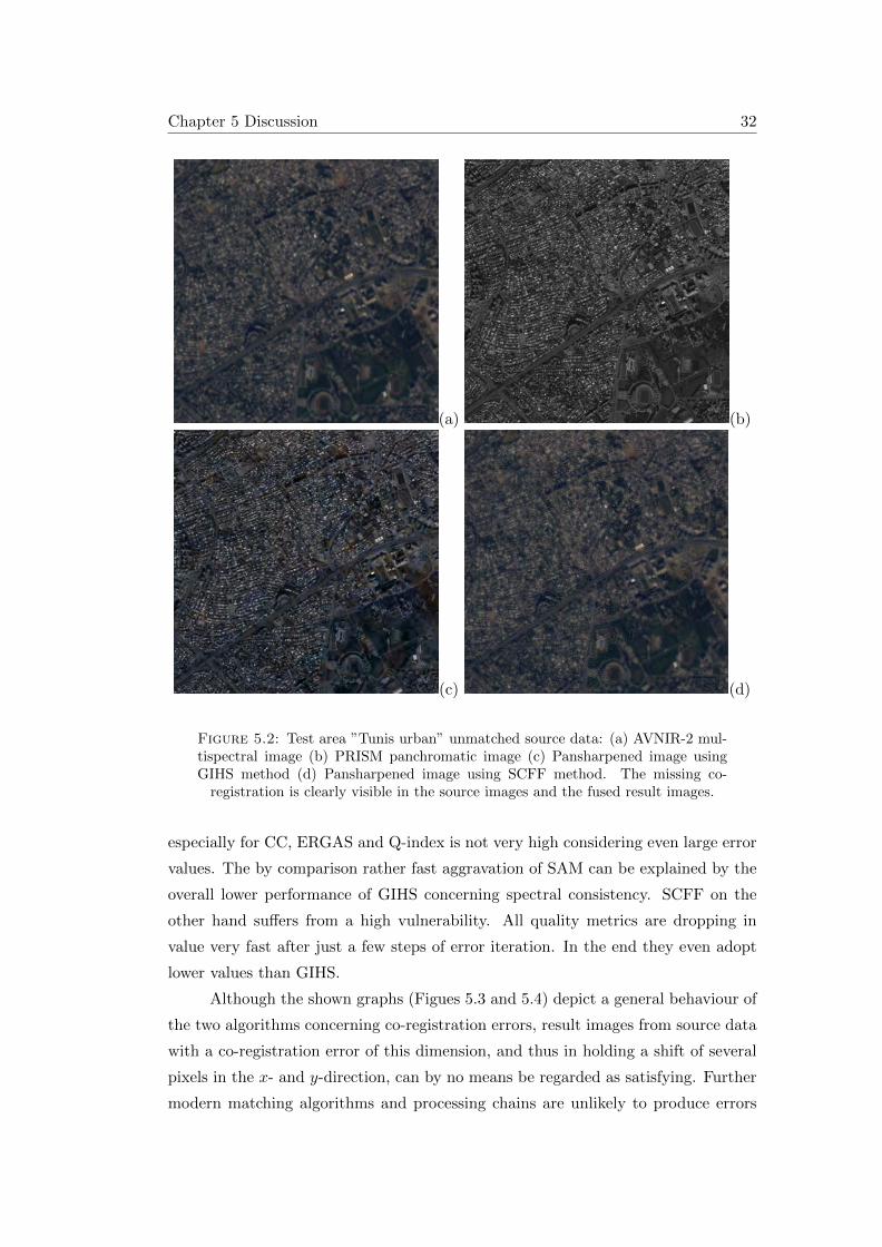
Figure 5.2: Test area ”Tunis urban” unmatched source data: (a) AVNIR-2 mul-tispectral image (b) PRISM panchromatic image (c) Pansharpened image usingGIHS method (d) Pansharpened image using SCFF method. The missing co-
registration is clearly visible in the source images and the fused result images.
especially for CC, ERGAS and Q-index is not very high considering even large error
values. The by comparison rather fast aggravation of SAM can be explained by the
overall lower performance of GIHS concerning spectral consistency. SCFF on the
other hand suffers from a high vulnerability. All quality metrics are dropping in
value very fast after just a few steps of error iteration. In the end they even adopt
lower values than GIHS.
Although the shown graphs (Figues 5.3 and 5.4) depict a general behaviour of
the two algorithms concerning co-registration errors, result images from source data
with a co-registration error of this dimension, and thus in holding a shift of several
pixels in the x- and y-direction, can by no means be regarded as satisfying. Further
modern matching algorithms and processing chains are unlikely to produce errors
Chapter 5 Discussion 33
to that degree. Typical image matching methods achieve results in the range of 0.2
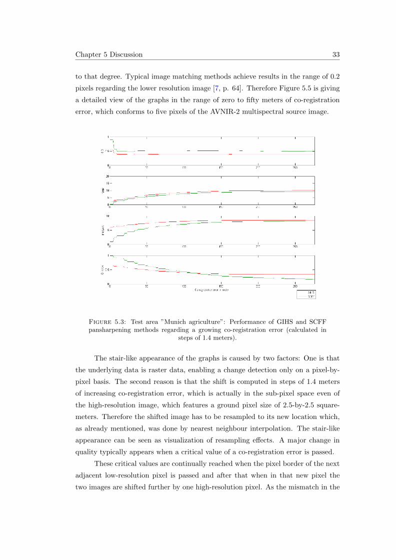
pixels regarding the lower resolution image [7, p. 64]. Therefore Figure 5.5 is giving
a detailed view of the graphs in the range of zero to fifty meters of co-registration
error, which conforms to five pixels of the AVNIR-2 multispectral source image.
Figure 5.3: Test area ”Munich agriculture”: Performance of GIHS and SCFFpansharpening methods regarding a growing co-registration error (calculated in
steps of 1.4 meters).
The stair-like appearance of the graphs is caused by two factors: One is that
the underlying data is raster data, enabling a change detection only on a pixel-by-
pixel basis. The second reason is that the shift is computed in steps of 1.4 meters
of increasing co-registration error, which is actually in the sub-pixel space even of
the high-resolution image, which features a ground pixel size of 2.5-by-2.5 square-
meters. Therefore the shifted image has to be resampled to its new location which,
as already mentioned, was done by nearest neighbour interpolation. The stair-like
appearance can be seen as visualization of resampling effects. A major change in
quality typically appears when a critical value of a co-registration error is passed.
These critical values are continually reached when the pixel border of the next
adjacent low-resolution pixel is passed and after that when in that new pixel the
two images are shifted further by one high-resolution pixel. As the mismatch in the
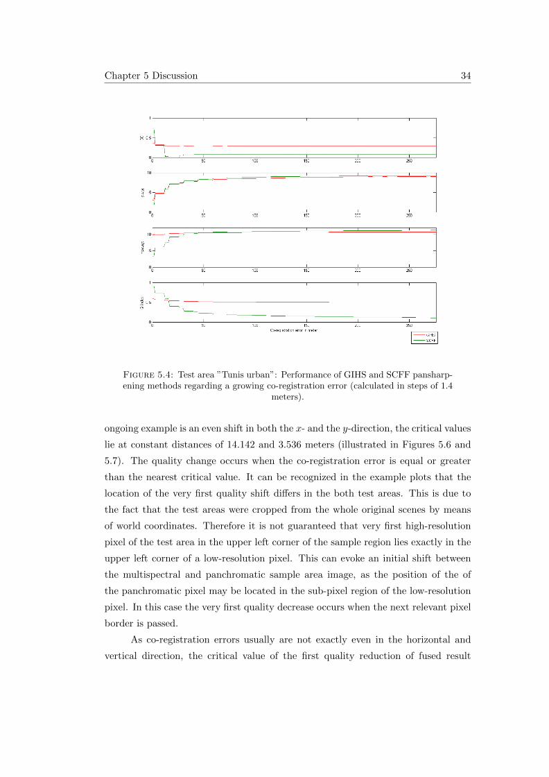
Chapter 5 Discussion 34
Figure 5.4: Test area ”Tunis urban”: Performance of GIHS and SCFF pansharp-ening methods regarding a growing co-registration error (calculated in steps of 1.4
meters).
ongoing example is an even shift in both the x- and the y-direction, the critical values
lie at constant distances of 14.142 and 3.536 meters (illustrated in Figures 5.6 and
5.7). The quality change occurs when the co-registration error is equal or greater
than the nearest critical value. It can be recognized in the example plots that the
location of the very first quality shift differs in the both test areas. This is due to
the fact that the test areas were cropped from the whole original scenes by means
of world coordinates. Therefore it is not guaranteed that very first high-resolution
pixel of the test area in the upper left corner of the sample region lies exactly in the
upper left corner of a low-resolution pixel. This can evoke an initial shift between
the multispectral and panchromatic sample area image, as the position of the of
the panchromatic pixel may be located in the sub-pixel region of the low-resolution
pixel. In this case the very first quality decrease occurs when the next relevant pixel
border is passed.
As co-registration errors usually are not exactly even in the horizontal and
vertical direction, the critical value of the first quality reduction of fused result
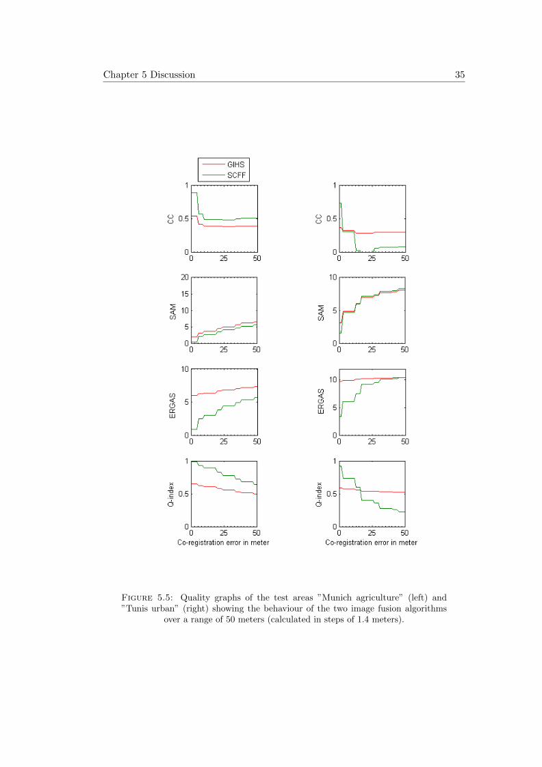
Chapter 5 Discussion 35
Figure 5.5: Quality graphs of the test areas ”Munich agriculture” (left) and”Tunis urban” (right) showing the behaviour of the two image fusion algorithms
over a range of 50 meters (calculated in steps of 1.4 meters).
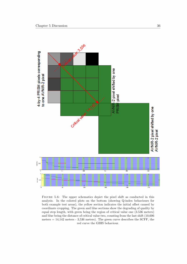
Chapter 5 Discussion 36
Figure 5.6: The upper schematics depict the pixel shift as conducted in thisanalysis. In the colored plots on the bottom (showing Q-index behaviours forboth example test areas), the yellow section indicates the initial offset caused bycoordinate cropping. The green and blue sections show the degrading of quality byequal step length, with green being the region of critical value one (3.536 meters)and blue being the distance of critical value two, counting from the last shift (10,606meters = 14,142 meters - 3,536 meters). The green curve describes the SCFF, the
red curve the GIHS behaviour.
Chapter 5 Discussion 37
images can be obtained as follows:
α = arcsin
√
Σ2L√
Σ2L + Σ2
G
CHRG =
PHRcosα
CHRL =PHRsinα
CLRG =PLRcosα
CLRL =PLRsinα
(5.1)
with
α = shift direction angle
ΣL = lesser shift value
ΣG = greater shift value
PHR = ground pixel edge length of high-resolution source image
PLR = ground pixel edge length of low-resolution source image
CHRG = high-resolution critical value in direction of the greater shift
CHRL = high-resolution critical value in direction of the lesser shift
CLEG = low-resolution critical value in direction of the greater shift
CLRL = low-resolution critical value in direction of the lesser shift.
As can be seen from the above equations the number of the continual quality
change doubles when the co-registration errors in the x- and y- direction are not
equal. Anyway the calculations in equation 5.1 only apply if the total error lies in
the sub-pixel space of the source high-resolution image. Image pairs with individ-
ual co-registration errors in x- and/or y-direction exceeding the ground-pixel size of
the panchromatic image can therefore be considered as inapplicable for pansharp-
ening processes. Concerning the performance of the two introduced image fusion
techniques, it can be stated that GIHS is the more stable method disregarding the
general and heavy influence of co-registration errors on the results.
The overall performance of the methods not only depends on the degree of
misregistration but also on the composition of the ground features. Areas with big
homogeneous surfaces, like the field test area of in Munich scene in Figure 5.1, tend
Chapter 5 Discussion 38
to degrade in quality by a slower rate than ground structures featuring a high spatial
frequency of image data.
5.2 Higher-level processing issues
With the characteristics of the two introduced satellite image fusion techniques con-
cerning co-registration errors of the source data being analyzed, one step further
is made by processing the result images to the next product level by applying AC
(atmospheric correction). The atmospheric corrected test areas are then classified
by means of index application of NDVI (Normalized Difference Vegetation Index)
and EVI (Enhanced Vegetation Index). The intention is to reveal which influence
the different degree of loss of spectral consistency concerning the two methods exerts
on post processing applications.
5.2.1 Atmospheric correction
The atmospheric correction is calculated using the ENVI/IDL module ATCOR,
based on the theoretical model for atmospheric correction of the same name, de-
veloped by Richter [9]. The whole process will only be summarized shortly as a
detailed view on the topic of atmospheric correction would go beyond the scope of
this work. In case of source image data originating from the PRISM and AVNIR-2
sensor following has to be considered. ”The standard rural (continental) aerosol
model is selected, because a reliable estimate of the aerosol type over land is not
possible with a few VNIR (visible and near infrared) channels. The influence of the
atmospheric water vapor column is very small for the AVNIR-2 channels, and since
a water vapor map cannot be derived from an AVNIR-2 scene, a typical seasonal/-
geographic value has to be taken. The same argument applies to the ozone column;
again a fixed value pertaining to the selected climatology of the MODTRAN stan-
dard atmospheres is used” [9, p. 4080]. For both scenes the ”Mid-Latitude Summer”
atmosphere model was used, featuring a water vapor column of 2.92 cm at sea level.
The general cycle of the atmospheric correction process can be layed out as:
1. Generation of masks for land, water, haze over land, cloud and satuared pixels
2. Calculation of aerosol optical thickness map at 550 nanometers
3. Optional haze removal
4. Application of surface reflectance retrieval
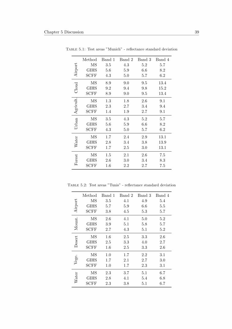
Chapter 5 Discussion 39
Table 5.1: Test areas ”Munich” - reflectance standard deviation
Method Band 1 Band 2 Band 3 Band 4
Air
port MS 3.5 4.3 5.2 5.7
GIHS 5.6 5.9 6.6 8.2SCFF 4.3 5.0 5.7 6.2
Clo
ud MS 8.9 9.0 9.5 13.4
GIHS 9.2 9.4 9.8 15.2SCFF 8.9 9.0 9.5 13.4
Agri
cult
.
MS 1.3 1.8 2.6 9.1GIHS 2.3 2.7 3.4 9.4SCFF 1.4 1.9 2.7 9.1
Urb
an MS 3.5 4.3 5.2 5.7
GIHS 5.6 5.9 6.6 8.2SCFF 4.3 5.0 5.7 6.2
Wat
er MS 1.7 2.4 2.9 13.1GIHS 2.8 3.4 3.8 13.9SCFF 1.7 2.5 3.0 13.1
For
est MS 1.5 2.1 2.6 7.5
GIHS 2.6 3.0 3.4 8.3SCFF 1.6 2.2 2.7 7.5
Table 5.2: Test areas ”Tunis” - reflectance standard deviation
Method Band 1 Band 2 Band 3 Band 4
Air
por
t MS 3.5 4.1 4.9 5.4GIHS 5.7 5.9 6.6 5.5SCFF 3.8 4.5 5.3 5.7
Mou
nt. MS 2.6 4.1 5.0 5.2
GIHS 3.9 5.1 5.8 5.7SCFF 2.7 4.3 5.1 5.2
Des
ert MS 1.6 2.5 3.3 2.6
GIHS 2.5 3.3 4.0 2.7SCFF 1.6 2.5 3.3 2.6
Veg
e. MS 1.0 1.7 2.2 3.1GIHS 1.7 2.1 2.7 3.0SCFF 1.0 1.7 2.3 3.1
Wat
er MS 2.3 3.7 5.1 6.7GIHS 2.8 4.1 5.4 6.8SCFF 2.3 3.8 5.1 6.7
Chapter 5 Discussion 40
As the individual calculations (e.g. water mask generation and water pixel de-
tection) of the atmospheric correction process especially highly depend on the data
contained in the blue and the near-infrared band of the processed image, ALOS
scenes again are very suitable for the evaluation of pansharpening performance in
relation to this type of higher-level processing. It was mentioned before that es-
pecially in these two channels the correlation between the multispectral and the
pancharomatic sensor is very low. Therefore a pansharpening method with a better
performance in the field of spectral consistency should be more capable to solve the
under-determined statistical problem of high-resolution spectral reconstruction and
thus deliver more consistent atmospheric correction results to the original multispec-
tral image.
Tables 5.1 and 5.2 show the results of the AC application. Product level 2A im-
ages are depicted with the processed source multispectral image being upsampled to
the size of the fused images by nearest-neighbour interpolation. The quality measure
hereby is the standard deviation of reflection calculated for each individual band.
The behaviour of GIHS and SCFF coincide with the insights got from the preced-
ing analysis concerning the influence of co-registration error. The SCFF constantly
delivers better results with some values even being equal to those of the original
AVNIR-2 test area, like in the cloud sample of the Munich scene and the desert,
vegetation and water samples of the Tunis scene. Atmospheric corrected images
based on GIHS fusion on the other hand throughoutly posses standard deviations of
reflection reaching values of 2.5 %. This difference between the two techniques again
is caused by their diverse approach on solving the pansharpening problem. In both
cases the highest difference values compared to the original multispectral image oc-
cur in band one and band four of the AVNIR-2 sensor which correspond to the blue
and the near-infrared channel. This again shows that the nature of the underlying
relative response functions of the involved optical satellite imaging sensors generally
influence the outcome of pansharpening processes.
5.2.2 Index application
While the analysis of the atmospheric correction applied to fused images revealed
that there are differences concerning the results of higher-level processing of variable
pansharpened satellite images, the unequal performance as displayed in the course
of this work can only be judged on a relative basis. Therefore the discussion in this
part showw the absolute influence of errors concerning the spectral consistency of
pansharpened images on classification based on atmospheric corrected source data.
Chapter 5 Discussion 41
5.2.2.1 NDVI and EVI
The NDVI (Normalized Difference Vegetation Index) is likely to be the most com-
monly used vegetation index in remote sensing applications. The NDVI is calculated
pixel-wise by following formular:
NDV I =NIR−RNIR+R
(5.2)
It shows the relative density of live vegetation on a ground patch of an optical
satellite remote sensing scene. As a relative indicator it can obtain values in the
interval of -1 to 1. As no still live vegetation causes NDVI values equal or nearing
zero and lower these values are generally omitted when visualizing the index.
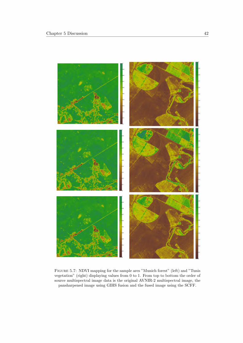
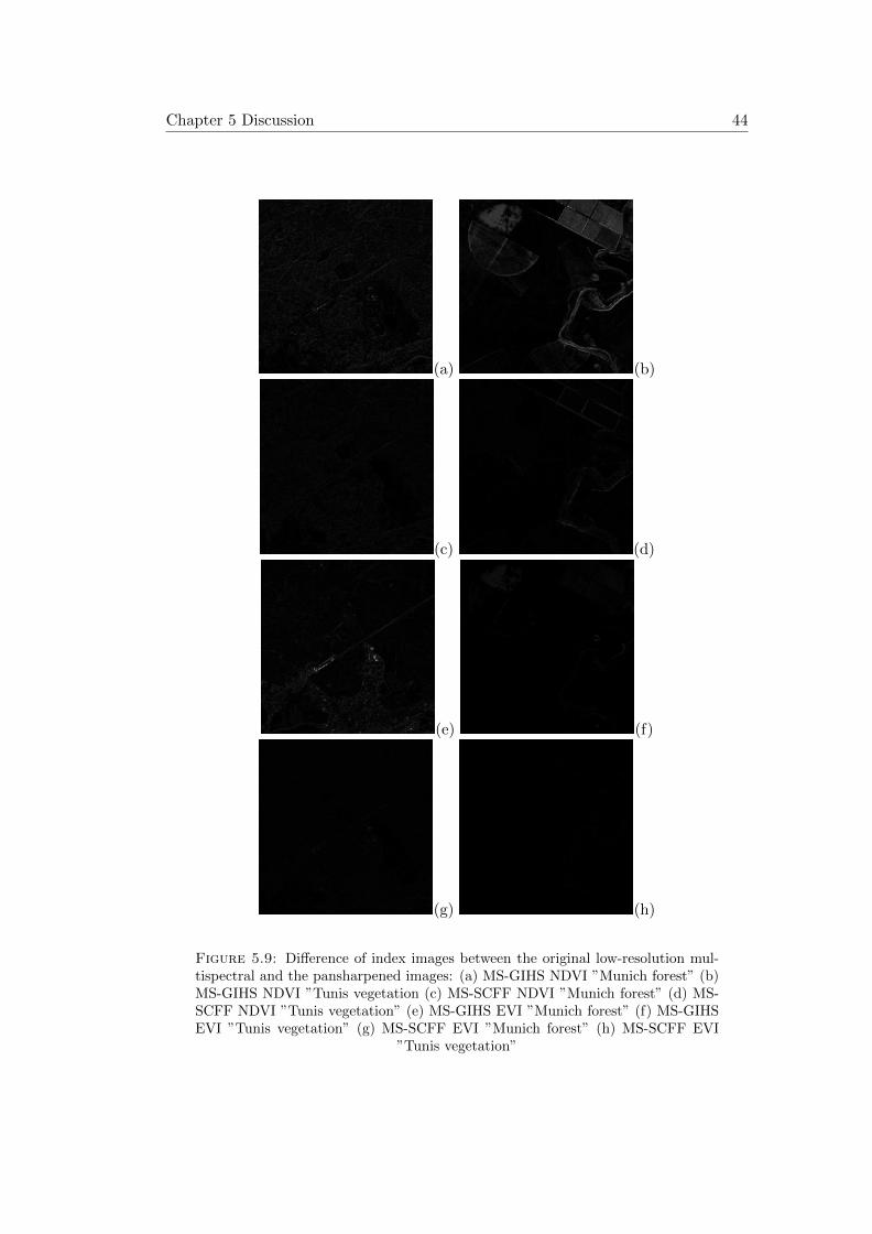
Viewing the images in Figure 5.7 depicting the results for the NDVI applica-
tion there is almost no significant difference recognizable. Only the GIHS version
of the test area from the Tunis scene appears to deliver slightly higher values for
the classification. In order to visualize potential differences, absolute difference im-
ages between the original multispectral NDVI image and the GIHS respectively the
SCFF NDVI image are calculated (Figure 5.9). These reveal that all presented pan-
sharpening method results suffer from (small) errors concerning index application.
Therefore it cannot be guaranteed that the fused images are suitable for higher-level
processing of this kind.
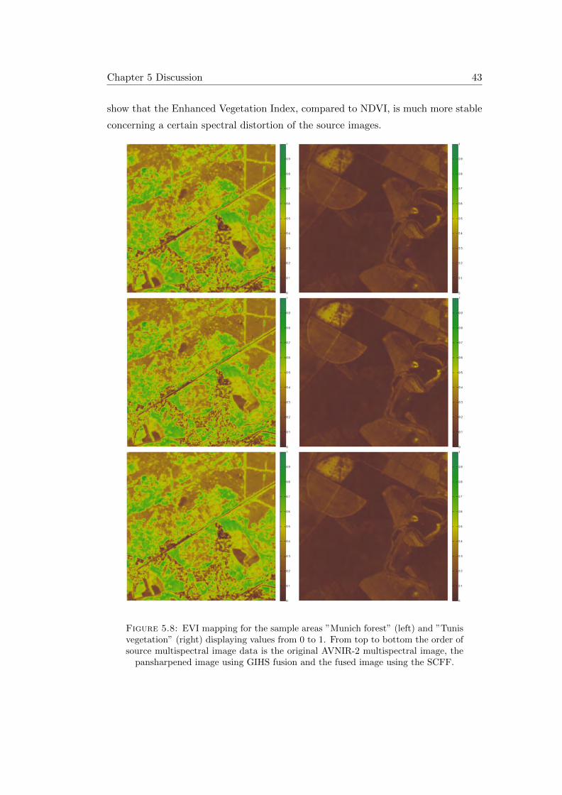
EVI (Enhanced Vegetation Index) is, as can be supposed by its name, an
improved vegetation index. It can be ”considered as a modified NDVI but with
improved sensitivity to high biomass regions and improved vegetation monitoring
capability through a decoupling of the canopy background signal and a reduction
in the atmospheric influences”[4, p. 1593f.]. The EVI value for every pixel in the
source image is obtain by the equation:
EV I = 2 ∗ NIR−RNIR+ C1 ∗R− C2 ∗B + L
(5.3)
withL = canopy background adjustment term
C1, C2 = coefficients of the aerosol resistance term(5.4)
As the ENVI remote sensing software was used to generate the EVI images, the
values for the coefficients L, C1 and C2 are respectively 1, 6 and 7.5. Looking at
equation 5.3 it is obvious that the calculation follows the same strategy as NDVI
and therefore relative ratios between the different multispectral bands are generated.
Concerning the results of the index application the difference images in Figure 5.9
Chapter 5 Discussion 42
Figure 5.7: NDVI mapping for the sample ares ”Munich forest” (left) and ”Tunisvegetation” (right) displaying values from 0 to 1. From top to bottom the order ofsource multispectral image data is the original AVNIR-2 multispectral image, the
pansharpened image using GIHS fusion and the fused image using the SCFF.
Chapter 5 Discussion 43
show that the Enhanced Vegetation Index, compared to NDVI, is much more stable
concerning a certain spectral distortion of the source images.
Figure 5.8: EVI mapping for the sample areas ”Munich forest” (left) and ”Tunisvegetation” (right) displaying values from 0 to 1. From top to bottom the order ofsource multispectral image data is the original AVNIR-2 multispectral image, the
pansharpened image using GIHS fusion and the fused image using the SCFF.
Chapter 5 Discussion 44
(a) (b)
(c) (d)
(e) (f)
(g) (h)
Figure 5.9: Difference of index images between the original low-resolution mul-tispectral and the pansharpened images: (a) MS-GIHS NDVI ”Munich forest” (b)MS-GIHS NDVI ”Tunis vegetation (c) MS-SCFF NDVI ”Munich forest” (d) MS-SCFF NDVI ”Tunis vegetation” (e) MS-GIHS EVI ”Munich forest” (f) MS-GIHSEVI ”Tunis vegetation” (g) MS-SCFF EVI ”Munich forest” (h) MS-SCFF EVI
”Tunis vegetation”
Chapter 6
Conclusion
In the course of this work inherent challenges of optical Earth observation satellite
image pansharpening were illustrated. They show that the quality of the results
concerning spectral and spatial consistency depends very much on the composition
of the source data and the used pansharpening principles of operation. Two dis-
tinctive methods, namely the Generalized Intensity-Hue-Saturation (GIHS) image
fusion and a Spectrally Consistent Fusion Framework (SCFF) were analyzed regard-
ing these aspects. It was discovered that SCFF consistently delivers more satisfying
results compared to GIHS, only suffering from a slightly increased loss of geometric
information. Typical quality indicators for the performance of image fusion were
introduced to assess the processes. The overall better performance of SCFF comes
with the drawback of a massively higher computation performance.
Further the influence of source data afflicted with co-registration errors was
evaluated by simulating a stepwise mismatch between the high-resolution panchro-
matic and the lower resolution multispectral image in the sub-pixel range of the
former. A general insight was gained that co-registration errors lying in the sub-
pixel range of the high-resolution image do not influence the pansharpening result
while errors of a greater margin decrease the quality very rapidly. This applies to
the experiments conducted in this thesis. In terms of the presented methods, GIHS
features a much higher stability concerning image mismatches.
Lastly the processing of the different pansharpening results to a higher product
level, by first conducting atmospheric correction and then applying two different veg-
etation indices, showed that spectral distortion caused by the pansharpening process
can but not necessarily will influence constitutive remote sensing applications.
While the tendencies of different pansharpening methods concerning a growing
co-registration error was observed from a scientific point of view, the practical use of
45
Chapter 6 Conclusion 46
optical satellite images mismatched to a greater extent can by denied. The results
of the distinctive techniques regarding properly registered data on the other hand
should not only be judged on quality metrics alone but also on the predetermined
intended purpose of use of the images.
There surely is much space for future experiments to build on and expand
the topic of this thesis. Constitutive analysis could observe the behaviour of other
common image fusion techniques concerning co-registration errors. Possible exam-
inations should also consider the development of robust pansharpening techniques
and new pansharpening approaches like the fusion of panchromatic, multispectral
and hyperspectral data or the combination of different optical satellite images with
non-optical satellite data like SAR (Synthetic Aperture Radar).
Bibliography
[1] Aanæs, H., Sveinsson, J.R., Nielsen, A.A., Bovith, T., and Benediktsson, J.A.,
2008: Model-based satellite image fusion. Geoscience and Remote Sensing,
IEEE Transactions on, 46(5):pages 1336–1346. doi:10.1109/TGRS.2008.916475.
[2] Aanæs, Henrik. http://www.imm.dtu.dk/∼aanes/. Accessed: 24-03-2014.
[3] Amro, Israa, Mateos, Javier, Vega, Miguel, Molina, Rafael, and Katsaggelos,
Aggelos K., 2011: A survey of classical methods and new trends in pansharpen-
ing of multispectral images. EURASIP J. Adv. Sig. Proc., 2011:pages 79–100.
[4] Chikr El-Mezouar, M., Taleb, N., Kpalma, K., and Ronsin, J., 2011: An
IHS-based fusion for color distortion reduction and vegetation enhancement in
IKONOS imagery. Geoscience and Remote Sensing, IEEE Transactions on,
49(5):pages 1590–1602. doi:10.1109/TGRS.2010.2087029.
[5] Earth Observation Research Center (EORC), Japan Aerospace Exploration
Agency (JAXA), 2-1-1, Sengen, Tsukuba-city, Ibaraki 305-8505 Japan, 2007:
ALOS User Handbook.
[6] Licciardi, GiorgioAntonino, Khan, MuhammadMurtaza, Chanussot, Jocelyn,
Montanvert, Annick, Condat, Laurent, and Jutten, Christian, 2012: Fusion of
hyperspectral and panchromatic images using multiresolution analysis and non-
linear pca band reduction. EURASIP Journal on Advances in Signal Processing,
2012(1):pages 1–17. doi:10.1186/1687-6180-2012-207.
[7] Muller, Rupert, Krauß, Thomas, Schneider, Mathias, and Reinartz, Peter, 2012:
Automated georeferencing of optical satellite data with integrated sensor model
improvement. Photogrammetric Engineering and Remote Sensing (PE&RS),
78(1):pages 61–74.
47
Bibliography 48
[8] Palubinskas, G. and Reinartz, P., 2011: Multi-resolution, multi-sensor image
fusion: general fusion framework. In Urban Remote Sensing Event (JURSE),
2011 Joint. pages 313–316. doi:10.1109/JURSE.2011.5764782.
[9] Schwind, P., Schneider, M., Palubinskas, G., Storch, T., Muller, R., and Richter,
R., 2009: Processors for alos optical data: Deconvolution, DEM generation,
orthorectification, and atmospheric correction. Geoscience and Remote Sens-
ing, IEEE Transactions on, 47(12):pages 4074–4082. doi:10.1109/TGRS.2009.
2015941.
[10] Tu, Te-Ming, Huang, P.S., Hung, Chung-Ling, and Chang, Chien-Ping, 2004:
A fast intensity-hue-saturation fusion technique with spectral adjustment for
IKONOS imagery. Geoscience and Remote Sensing Letters, IEEE, 1(4):pages
309–312. doi:10.1109/LGRS.2004.834804.
[11] Tu, Te-Ming, Su, Shun-Chi, Shyu, Hsuen-Chyun, and Huang, Ping S., 2001:
A new look at IHS-like image fusion methods. Information Fusion, 2(3):pages
177–186. doi:http://dx.doi.org/10.1016/S1566-2535(01)00036-7.
[12] Wald, L., 1997: Fusion of satellite images of different spatial resolutions: as-
sessing the quality of resulting images. volume 63. pages 691–699.
[13] Wald, L., 2000: Quality of high resolution synthesised images: Is there a sim-
ple criterion ? In proceedings of the third conference ”Fusion of Earth data:
merging point measurements, raster maps and remotely sensed images”, Sophia
Antipolis, France. pages 99–103.
[14] Wang, Zhou and Bovik, A.C., 2002: A universal image quality index. Signal
Processing Letters, IEEE, 9(3):pages 81–84. doi:10.1109/97.995823.
[15] Yuhas R.H., Boardman J.W., Goetz A.F.H., 1992: Discrimination among
semi-arid landscape endmembers using the spectral angle mapper (sam) algo-
rithm:pages 147–149.
[16] Zhu, X.X. and Bamler, R., 2013: A sparse image fusion algorithm with appli-
cation to pan-sharpening. Geoscience and Remote Sensing, IEEE Transactions
on, 51(5):pages 2827–2836. doi:10.1109/TGRS.2012.2213604.