on the impact of variability and assembly on turbine blade

On the Impact of Variability and Assembly on Turbine Blade

Cooling Flow and Oxidation Life

by

Carroll Vincent Sidwell

B.E., Vanderbilt University (1994)M.S., Vanderbilt University (1996)

Submitted to the Department of Aeronautics and Astronauticsin partial fulfillment of the requirements for the degree of

Doctor of Philosophy

at the

MASSACHUSETTS INSTITUTE OF TECHNOLOGY

June 2004

c© Massachusetts Institute of Technology 2004. All rights reserved.

Author . . . . . . . . . . . . . . . . . . . . . . . . . . . . . . . . . . . . . . . . . . . . . . . . . . . . . . . . . . . . . . . . . . . . . . . . . . . .Department of Aeronautics and Astronautics

May 7, 2004

Certified by. . . . . . . . . . . . . . . . . . . . . . . . . . . . . . . . . . . . . . . . . . . . . . . . . . . . . . . . . . . . . . . . . . . . . . . .David L. Darmofal

Associate Professor of Aeronautics and AstronauticsThesis Supervisor

Certified by. . . . . . . . . . . . . . . . . . . . . . . . . . . . . . . . . . . . . . . . . . . . . . . . . . . . . . . . . . . . . . . . . . . . . . . .Alan H. Epstein

R.C. Maclaurin Professor of Aeronautics and Astronautics

Certified by. . . . . . . . . . . . . . . . . . . . . . . . . . . . . . . . . . . . . . . . . . . . . . . . . . . . . . . . . . . . . . . . . . . . . . . .Edward M. Greitzer

H.N. Slater Professor of Aeronautics and Astronautics

Certified by. . . . . . . . . . . . . . . . . . . . . . . . . . . . . . . . . . . . . . . . . . . . . . . . . . . . . . . . . . . . . . . . . . . . . . . .Jayant S. Sabnis

Director of Aerodynamics, Pratt & Whitney

Certified by. . . . . . . . . . . . . . . . . . . . . . . . . . . . . . . . . . . . . . . . . . . . . . . . . . . . . . . . . . . . . . . . . . . . . . . .Ian A. Waitz

Professor of Aeronautics and Astronautics

Accepted by . . . . . . . . . . . . . . . . . . . . . . . . . . . . . . . . . . . . . . . . . . . . . . . . . . . . . . . . . . . . . . . . . . . . . . .Edward M. Greitzer

H.N. Slater Professor of Aeronautics and AstronauticsChair, Committee on Graduate Students

On the Impact of Variability and Assembly on Turbine Blade Cooling

Flow and Oxidation Life

by

Carroll Vincent Sidwell

Submitted to the Department of Aeronautics and Astronauticson May 7, 2004, in partial fulfillment of the

requirements for the degree ofDoctor of Philosophy

Abstract

The life of a turbine blade is dependent on the quantity and temperature of the cooling flow sup-plied to the blade. The focus of this thesis is the impact of variability on blade cooling flow and,subsequently, its impact on oxidation life. A probabilistic analysis is performed on a commercialjet engine to quantify the variability in blade flow and oxidation life due to variability in ambientconditions, main gaspath conditions, the cooling air delivery system, and the flow capability of theblade internal cooling passages. The probabilistic analysis is used to demonstrate that every bladein a turbine row must be individually modeled in order to accurately estimate the distribution ofblade-row oxidation life for a population of jet engines. In particular, since the oxidation life of ablade row is limited by the highest temperature (and therefore lowest-flowing) blades, every blademust be individually represented to correctly model (1) the probability of observing (within a row) ablade with a low coolant flow capability, and (2) the flow rate (and therefore the metal temperatureand life) of these passages. A simplified flow network model of the cooling air supply system anda row of blades is proposed which agrees qualitatively and quantitatively with the more complexflow network model of the entire jet engine. Using this simplified model, the controlling parame-ters which affect the distribution of cooling flow in a blade row are identified. Finally, a selectiveassembly method is proposed to decrease the impact of blade passage manufacturing variability onblade flow. The method classifies blades into groups based on passage flow capability and assemblesrows from within the groups. As a result, the flow and the oxidation life improve for the majorityof blade rows, while segregating low-flow blades into sets that are no worse than random assembly.Alternatively, selective assembly can be used to allow blades to withstand increased turbine inlettemperature while maintaining the maximum blade metal temperature at random-assembly levels.

Thesis Supervisor: David L. DarmofalTitle: Associate Professor of Aeronautics and Astronautics

3

Acknowledgments

I would like to thank Professor David Darmofal, who provided invaluable guidance, motivation, and

support for the duration of my doctoral studies. I would also like to thank my doctoral committee

for their guidance, including Professor Alan Epstein, Professor Edward Greitzer, Dr. Jayant Sabnis

(Pratt & Whitney), and Professor Ian Waitz. In addition, I thank the faculty and students on the

MIT Robust Jet Engines team for their input and assistance, especially Professor Daniel Frey and

John Hsia.

I would like to thank Pratt & Whitney for providing the financial support and flexibility to

allow me to pursue my doctoral degree, particularly Gordon Pickett, Mark Zelesky, Brent Staubach,

David Pack, and Ed Crow who all played critical roles that enabled this to take place. There are also

numerous people at Pratt & Whitney that have generously offered technical expertise and assistance

throughout this research, in particular David Candelori, David Cloud, and Ping Dang.

I would like to thank my family and friends for their support over the last few years, especially

my wife, Nicole. Without her patience, understanding, and support, I never could have succeeded.

Finally, thanks to Katie for making me keep things in perspective.

5

Contents

1 Introduction 11

1.1 Motivation . . . . . . . . . . . . . . . . . . . . . . . . . . . . . . . . . . . . . . . . . 11

1.2 Thesis Objectives . . . . . . . . . . . . . . . . . . . . . . . . . . . . . . . . . . . . . . 15

1.3 Background . . . . . . . . . . . . . . . . . . . . . . . . . . . . . . . . . . . . . . . . . 15

1.4 Outline . . . . . . . . . . . . . . . . . . . . . . . . . . . . . . . . . . . . . . . . . . . 18

1.5 Contributions . . . . . . . . . . . . . . . . . . . . . . . . . . . . . . . . . . . . . . . . 19

2 Probabilistic Analysis of a Turbine Cooling Air Delivery System 21

2.1 Introduction . . . . . . . . . . . . . . . . . . . . . . . . . . . . . . . . . . . . . . . . . 21

2.2 Flow Network Analysis . . . . . . . . . . . . . . . . . . . . . . . . . . . . . . . . . . . 22

2.3 Blade Oxidation Life Estimation . . . . . . . . . . . . . . . . . . . . . . . . . . . . . 24

2.4 Probabilistic Analysis . . . . . . . . . . . . . . . . . . . . . . . . . . . . . . . . . . . 26

2.5 Probabilistic Analysis Results . . . . . . . . . . . . . . . . . . . . . . . . . . . . . . . 30

2.6 Identification of Key Noise Sources . . . . . . . . . . . . . . . . . . . . . . . . . . . . 35

2.7 Summary . . . . . . . . . . . . . . . . . . . . . . . . . . . . . . . . . . . . . . . . . . 38

3 Behavior of Cooling Air Supply Systems Including Blade Flow Variability 41

3.1 Introduction . . . . . . . . . . . . . . . . . . . . . . . . . . . . . . . . . . . . . . . . . 41

3.2 Simplified Model of a Flow System with Single-Passage Blades . . . . . . . . . . . . 42

3.3 Selective Assembly Method to Reduce Blade Flow Variability . . . . . . . . . . . . . 44

3.4 Behavior of “Lumped” Blades . . . . . . . . . . . . . . . . . . . . . . . . . . . . . . . 45

3.5 Effect of Multi-Passage Blades . . . . . . . . . . . . . . . . . . . . . . . . . . . . . . 46

3.6 Impact of Selective Assembly on Turbine Inlet Temperature . . . . . . . . . . . . . . 50

3.7 Summary . . . . . . . . . . . . . . . . . . . . . . . . . . . . . . . . . . . . . . . . . . 54

4 Application of Selective Assembly to a Commercial Turbofan 57

4.1 Introduction . . . . . . . . . . . . . . . . . . . . . . . . . . . . . . . . . . . . . . . . . 57

4.2 Characterization of the Cooling Air Supply System . . . . . . . . . . . . . . . . . . . 58

7

4.3 Definition of Selective Assembly Classes . . . . . . . . . . . . . . . . . . . . . . . . . 58

4.4 Results of Selective Assembly . . . . . . . . . . . . . . . . . . . . . . . . . . . . . . . 58

4.5 Impact of Selective Assembly on Performance . . . . . . . . . . . . . . . . . . . . . . 65

4.6 Summary . . . . . . . . . . . . . . . . . . . . . . . . . . . . . . . . . . . . . . . . . . 66

5 Summary and Recommendations 69

5.1 Summary . . . . . . . . . . . . . . . . . . . . . . . . . . . . . . . . . . . . . . . . . . 69

5.2 Recommendations for Future Work . . . . . . . . . . . . . . . . . . . . . . . . . . . . 70

A Correlated and Classified Random Variables 73

A.1 Truncated Normal Distribution . . . . . . . . . . . . . . . . . . . . . . . . . . . . . . 73

A.2 Correlated Variables With Classification . . . . . . . . . . . . . . . . . . . . . . . . . 73

8

List of Figures

1-1 Historical trend in specific core power and turbine rotor inlet temperature for a variety

of military and commercial gas turbine engines . . . . . . . . . . . . . . . . . . . . . 12

1-2 Graph of turbine rotor inlet temperature versus year of entry into service for military

engines . . . . . . . . . . . . . . . . . . . . . . . . . . . . . . . . . . . . . . . . . . . . 12

1-3 Histograms of oxidation life field data for two airlines and cumulative probability

distributions of oxidation life . . . . . . . . . . . . . . . . . . . . . . . . . . . . . . . 14

1-4 Cross section of a commercial turbofan, highlighting the auxiliary air system . . . . 16

1-5 Histogram of blade leading-edge flow capability as measured during manufacture . . 17

2-1 Schematic cross section of area of interest, including the aft portion of the combustor

and the first stage of the high-pressure turbine . . . . . . . . . . . . . . . . . . . . . 23

2-2 Schematic cross section of area of interest, including the aft portion of the combustor

and the first stage of the high-pressure turbine, showing a portion of network flow

model . . . . . . . . . . . . . . . . . . . . . . . . . . . . . . . . . . . . . . . . . . . . 28

2-3 Histograms of blade leading-edge passage, midbody passage, and trailing-edge passage

flow capability . . . . . . . . . . . . . . . . . . . . . . . . . . . . . . . . . . . . . . . 29

2-4 Histograms showing the distribution of blade leading-edge passage flow for all the

blades in a fleet and the lowest-flow blades in each blade row . . . . . . . . . . . . . 31

2-5 Probability density functions comparing Airline A and Airline B for: (1) field failure

data, (2) nominal analyses with historical variability, and (3) probabilistic analyses . 32

2-6 Results of hypothesis tests comparing field data to probabilistic analyses and nominal

analyses for Airline A and Airline B . . . . . . . . . . . . . . . . . . . . . . . . . . . 34

2-7 Relationship between blade row reference life and the number of failed blades required

for a blade row failure . . . . . . . . . . . . . . . . . . . . . . . . . . . . . . . . . . . 35

2-8 Changes in typical and minimum life that result from a 10% decrease in each variable’s

standard deviation superimposed on typical and minimum life . . . . . . . . . . . . . 39

9

3-1 Simplified model of a turbine cooling air supply system and a row of n cooled turbine

blades . . . . . . . . . . . . . . . . . . . . . . . . . . . . . . . . . . . . . . . . . . . . 43

3-2 Schematic of a simplified turbine cooling air supply system where each blade consists

of two passages . . . . . . . . . . . . . . . . . . . . . . . . . . . . . . . . . . . . . . . 47

3-3 Histograms of passage areas, blade plenum pressure, individual blade flow, and the

lowest blade flow in each blade row for three levels of area correlation from the two

passage simplified model . . . . . . . . . . . . . . . . . . . . . . . . . . . . . . . . . . 51

3-4 The distribution of manufactured flow capability is divided into three flow classes for

demonstration of selective assembly of turbine blade rows . . . . . . . . . . . . . . . 53

3-5 Estimated increase in turbine inlet temperature as a function of β for three different

levels of nominal overall cooling effectiveness . . . . . . . . . . . . . . . . . . . . . . 54

3-6 Estimated increase in turbine inlet temperature as a function of β for three blade flow

classes, each with a nominal overall cooling effectiveness . . . . . . . . . . . . . . . . 55

3-7 Estimated increase in turbine inlet temperature as a function of β for three levels of

inter-passage correlation, each with a nominal overall cooling effectiveness . . . . . . 56

4-1 The distribution of manufactured flow capability is divided into three flow classes

(Low-Flow, Nominal-Flow, and High-Flow) for demonstration of selective assembly of

turbine blade rows . . . . . . . . . . . . . . . . . . . . . . . . . . . . . . . . . . . . . 59

4-2 Histograms showing blade plenum pressure for randomly assembled and selectively

assembled blade rows . . . . . . . . . . . . . . . . . . . . . . . . . . . . . . . . . . . . 60

4-3 Histograms showing blade leading-edge passage flow for all blades in all rows for

random and selective assembly . . . . . . . . . . . . . . . . . . . . . . . . . . . . . . 61

4-4 Histograms showing minimum blade leading-edge passage flow in each blade row for


4-5 Histograms showing the maximum blade metal temperature in each blade row for


4-6 Histograms showing the minimum blade life in each blade row for random and selective

assembly . . . . . . . . . . . . . . . . . . . . . . . . . . . . . . . . . . . . . . . . . . . 64

4-7 Histograms showing the total flow delivered to the blade row for random and selective

assembly . . . . . . . . . . . . . . . . . . . . . . . . . . . . . . . . . . . . . . . . . . . 65

10

Chapter 1

Introduction

1.1 Motivation

Since their inception in the late 1930’s, the specific core power of gas turbines has increased over

600%, from 50 hplb/sec for Whittle’s W2 to greater than 300 hp

lb/sec for modern engines like the GE90

or PW4084 [21]. This evolution in performance is closely related to increases in turbine rotor inlet

temperature as the performance of modern gas turbine engines improves with increased turbine

inlet temperature. For an ideal turbofan, for example, increases in turbine inlet temperature produce

increased thrust and increased specific impulse [20]. Figure 1-1 shows that turbine inlet temperature

has increased roughly 1600◦F in 60 years. However, much of that improvement occurred during the

middle of the twentieth century. Figure 1-2 shows that the state-of-the-art in turbine rotor inlet

temperature increased 1100◦F between 1960 and 1980 (about 55◦F per year), compared to only

100◦F between 1980 and 1997 (about 6◦F per year) [43]. The desire for better performance and

improved efficiency will continue the trend toward higher turbine inlet temperatures, as current

engine technology limits turbine temperatures to those well below stoichiometric combustion limits

[21].

High turbine inlet temperatures provide a challenging environment for turbine blades which are

subject to a variety of damage mechanisms, including high-temperature oxidation, creep, corrosion,

and thermo-mechanical fatigue. Thus, engine designs must strike a balance between thermodynamic

performance and component life. In response, turbine airfoil temperature capability has evolved

on two fronts: materials and airfoil cooling. The metal temperature capability of turbine airfoil

materials has improved more than 500◦F in the last 50 years [21]. However, advancements in

turbine blade cooling have allowed an even larger increase. Newer-generation turbine airfoils operate

at turbine-rotor inlet temperatures that are 1200◦F above those of comparable uncooled blades and

600◦F above the incipient melting temperature of the alloys [21].

11

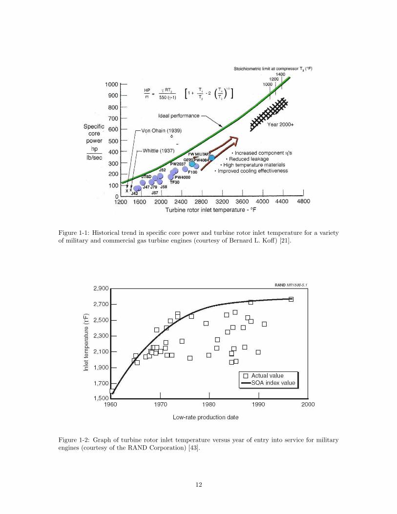
Figure 1-1: Historical trend in specific core power and turbine rotor inlet temperature for a varietyof military and commercial gas turbine engines (courtesy of Bernard L. Koff) [21].

Figure 1-2: Graph of turbine rotor inlet temperature versus year of entry into service for militaryengines (courtesy of the RAND Corporation) [43].

12

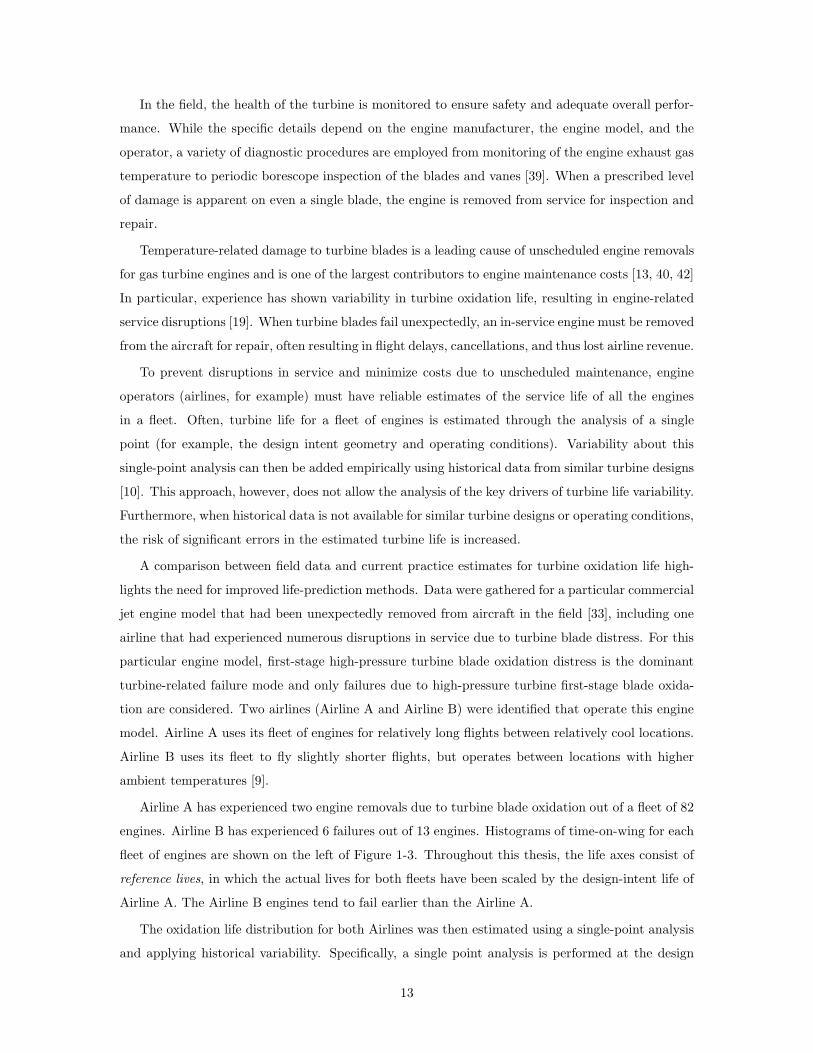
In the field, the health of the turbine is monitored to ensure safety and adequate overall perfor-

mance. While the specific details depend on the engine manufacturer, the engine model, and the

operator, a variety of diagnostic procedures are employed from monitoring of the engine exhaust gas

temperature to periodic borescope inspection of the blades and vanes [39]. When a prescribed level

of damage is apparent on even a single blade, the engine is removed from service for inspection and

repair.

Temperature-related damage to turbine blades is a leading cause of unscheduled engine removals

for gas turbine engines and is one of the largest contributors to engine maintenance costs [13, 40, 42]

In particular, experience has shown variability in turbine oxidation life, resulting in engine-related

service disruptions [19]. When turbine blades fail unexpectedly, an in-service engine must be removed

from the aircraft for repair, often resulting in flight delays, cancellations, and thus lost airline revenue.

To prevent disruptions in service and minimize costs due to unscheduled maintenance, engine

operators (airlines, for example) must have reliable estimates of the service life of all the engines

in a fleet. Often, turbine life for a fleet of engines is estimated through the analysis of a single

point (for example, the design intent geometry and operating conditions). Variability about this

single-point analysis can then be added empirically using historical data from similar turbine designs

[10]. This approach, however, does not allow the analysis of the key drivers of turbine life variability.

Furthermore, when historical data is not available for similar turbine designs or operating conditions,

the risk of significant errors in the estimated turbine life is increased.

A comparison between field data and current practice estimates for turbine oxidation life high-

lights the need for improved life-prediction methods. Data were gathered for a particular commercial

jet engine model that had been unexpectedly removed from aircraft in the field [33], including one

airline that had experienced numerous disruptions in service due to turbine blade distress. For this

particular engine model, first-stage high-pressure turbine blade oxidation distress is the dominant

turbine-related failure mode and only failures due to high-pressure turbine first-stage blade oxida-

tion are considered. Two airlines (Airline A and Airline B) were identified that operate this engine

model. Airline A uses its fleet of engines for relatively long flights between relatively cool locations.

Airline B uses its fleet to fly slightly shorter flights, but operates between locations with higher

ambient temperatures [9].

Airline A has experienced two engine removals due to turbine blade oxidation out of a fleet of 82

engines. Airline B has experienced 6 failures out of 13 engines. Histograms of time-on-wing for each

fleet of engines are shown on the left of Figure 1-3. Throughout this thesis, the life axes consist of

reference lives, in which the actual lives for both fleets have been scaled by the design-intent life of

Airline A. The Airline B engines tend to fail earlier than the Airline A.

The oxidation life distribution for both Airlines was then estimated using a single-point analysis

and applying historical variability. Specifically, a single point analysis is performed at the design

13

0 0.2 0.40

2

4

6

8

10

12

Reference Life

Num

ber

of E

ngin

es

Airline A

Non−FailuresFailures

0 0.2 0.40

1

2

3

4

5

Reference Life

Num

ber

of E

ngin

es

Airline B

Non−FailuresFailures

0 0.5 1 1.5 20

0.25

0.5

0.75

1

Reference Life

Cum

ulat

ive

Pro

babi

lity

Airline A

Nom. w/ Historical VariabilityNominal Life

0 0.5 1 1.5 20

0.25

0.5

0.75

1

Reference Life

Cum

ulat

ive

Pro

babi

lity

Airline B

Nom. w/ Historical VariabilityNominal Life

Figure 1-3: Histograms of oxidation life field data for two airlines and cumulative probability distri-butions of oxidation life that are generated using nominal analysis and historical variability [33].

intent geometry and operating conditions (using the analysis described in detail in Chapter 2).

Weibull probability distributions with historically-based slopes are then used to model the expected

distributions of oxidation life for the Airlines [1, 23]. The right side of Figure 1-3 shows the resulting

Weibull cumulative distribution functions for Airline A and B.

For Airline A the nominal estimate including historical variability is in reasonable agreement

with the observed field failure rate, while for Airline B the estimate including historical variability

predicts a much lower probability of failure than observed in the field. For example, Airline A field

data show a failure probability of 2.4% (2 out of 82 engines). The nominal analysis with historical

variability suggests that the failure rate would be 3.2% at a reference life of 0.4 (which is the largest

life observed in Airline A data). The reasonable agreement between the Airline A field data and the

nominal analysis with historical variability is expected because the historical variability is derived

from field data for engines and operating conditions which are similar to Airline A. In contrast,

14

Airline B shows that nearly half its fleet has failed around a reference life of 0.2. The nominal

analysis with historical variability indicates that Airline B should expect no failures by a reference

life of 0.2.

1.2 Thesis Objectives

The preceding example shows that the estimation of turbine oxidation life based on design intent

analysis and historical variability is not accurate for all operators. Further, since historical data is

utilized to estimate the variability in turbine life, this approach precludes the identification of the

key parameters that control the variability of turbine life for a fleet of engines. In this thesis, these

shortcomings are addressed through the application of probabilistic analysis to the turbine cooling

system. The main objectives of this thesis are:

• To quantify the variability in blade flow and oxidation life due to variability in ambient condi-

tions, main gaspath conditions, the cooling air delivery system, and the effective areas of the

internal blade passages using probabilistic analysis.

• To identify the controlling parameters and key drivers of variability in blade cooling flow and

oxidation using probabilistic analysis.

• To develop a methodology to increase engine time-on-wing, as limited by blade oxidation.

1.3 Background

Typical modern turbine blades rely on relatively cooler air from the high-pressure compressor to

continually remove the heat absorbed from the main gaspath. The auxiliary air system delivers this

cooling air to the turbine blades and vanes. The dominant methods of heat transfer are internal con-

vection cooling, impingement cooling, and film cooling. Convection cooling involves passing cooling

air through roughened internal passages in a blade to decrease metal temperature. Impingement

cooling is similar to convection, except that internal cooling air is channeled to directly impinge on

the inside face of a blade’s exterior wall, increasing the heat transfer from the airfoil wall to the

cooling air. Finally, film cooling uses numerous small holes drilled through the outer wall of the

airfoil to lay a thin film of cool air on the outer surface of the blade, insulating the blade from the

hot gas path flow. Most modern high-pressure turbine blades and vanes employ all three cooling

strategies [18]. An overview of turbine blade durability design can be found in Kerrebrock [20] and

Cohen et al. [12]. A more in-depth treatment can be found in Han [18].

As a testament to its importance, the last few decades have seen an enormous amount of research

related to turbine airfoil cooling. In 1971, Goldstein published an early survey of film cooling research

15

that included 72 studies [15]. In contrast, in 2000, Han et al. published a text on turbine cooling

including citations of hundreds of research papers [18]. Turbine cooling continues to be an active

area of research for both industry and academia.

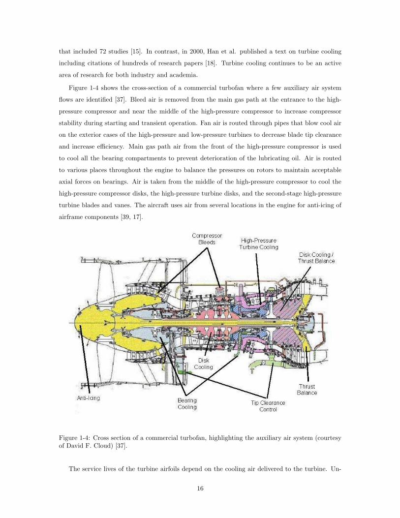
Figure 1-4 shows the cross-section of a commercial turbofan where a few auxiliary air system

flows are identified [37]. Bleed air is removed from the main gas path at the entrance to the high-

pressure compressor and near the middle of the high-pressure compressor to increase compressor

stability during starting and transient operation. Fan air is routed through pipes that blow cool air

on the exterior cases of the high-pressure and low-pressure turbines to decrease blade tip clearance

and increase efficiency. Main gas path air from the front of the high-pressure compressor is used

to cool all the bearing compartments to prevent deterioration of the lubricating oil. Air is routed

to various places throughout the engine to balance the pressures on rotors to maintain acceptable

axial forces on bearings. Air is taken from the middle of the high-pressure compressor to cool the

high-pressure compressor disks, the high-pressure turbine disks, and the second-stage high-pressure

turbine blades and vanes. The aircraft uses air from several locations in the engine for anti-icing of

airframe components [39, 17].

Figure 1-4: Cross section of a commercial turbofan, highlighting the auxiliary air system (courtesyof David F. Cloud) [37].

The service lives of the turbine airfoils depend on the cooling air delivered to the turbine. Un-

16

fortunately, the temperature, pressure, and flow rate of the cooling air are susceptible to variability.

This variation in the cooling air can lead to increases in component metal temperatures and sub-

sequent decreases in life. The cooling air delivery system should provide cooling air at the lowest

possible temperature and the highest possible pressure.

One source of variability in the cooling flow is due to the manufacturing of the blades [39].

Typical internally-cooled, modern turbine airfoils are investment-cast as single crystals of nickel-

based superalloy. Numerous cooling holes are drilled through the surface of the airfoil, using either

laser-drilling or electro-discharge machining [39]. The casting and hole-drilling processes are both

difficult to control, resulting in part-to-part variation in coolant mass flow capability. In general,

large variations are accepted due to the high cost of manufacture for these parts. After the airfoils

are manufactured, they are flowed under controlled conditions to ensure they pass an acceptable

amount of coolant flow at a given pressure ratio. Figure 1-5 shows a histogram of blade leading-edge

flow capability measured during manufacture, normalized by the design-intent flow capability, where

the demonstrated variability in flow is several percent [31]. The accepted blades are then assembled

randomly into a row.

0.9 0.95 1 1.05 1.1Measured Leading−Edge Passage Flow Capability

Figure 1-5: Histogram of blade leading-edge flow capability as measured during manufacture (nor-malized by the design-intent flow capability)[31].

Other potential sources of blade cooling flow variability exist upstream of the blades. For ex-

ample, cooling air for the first-stage turbine blades comes from the main gas path near the exit of

the high-pressure compressor. The cooling air travels a complicated path from the exit of the high-

pressure compressor, through static ducting, between rotating parts, and finally through the internal

17

passages of rotating blades. All of these features are subject to manufacturing variation, potentially

altering the cooling air quantity and character. In addition, day-to-day operational variability, such

as ambient temperature and takeoff altitude, can affect the cooling air supply by changing the gas

path temperatures, pressures, and rotational speeds.

The application of probabilistic methods to gas turbine engines is not new. In particular, the last

two decades have seen a surge in the application of probabilistic analysis to gas turbine engines. Much

of the early work was driven primarily by the desire to eliminate particularly dangerous failure modes

such as catastrophic disk burst while enabling the design of higher-performance engines. In 2002,

Garzon summarized the application of probabilistic techniques to gas turbine structural analysis

and noted that engine manufacturers are increasingly using probabilistic analysis to improve engine

design [14]. Recently, however, it is becoming clear that significant performance gains will be difficult

to achieve without consideration of the uncertainties present in the analysis and design of gas turbine

engines [8]. Somewhat surprisingly, relatively little research has focused on probabilistic aerothermal

design of gas turbine engines, likely due to the complex nature of the physical phenomena [14].

Mavris, along with various colleagues, has addressed some probabilistic aerothermal issues, including

creep life assessment of turbine blades with varying operating conditions [24], thrust sizing for

an unmanned aerial combat vehicle with mission uncertainty [34], and the effect of uncertainty

in engine component performance on overall engine performance [26, 27]. Abumeri and Chamis

used probabilistic methods to analyze the impact of different compressor and turbine designs on

the mission performance of a conceptual supersonic aircraft [2]. Recently, Garzon addressed the

probabilistic aerothermal design of compressor airfoils by quantifying the manufacturing variation

in compressor airfoil shape and its effect on compressor performance [14].

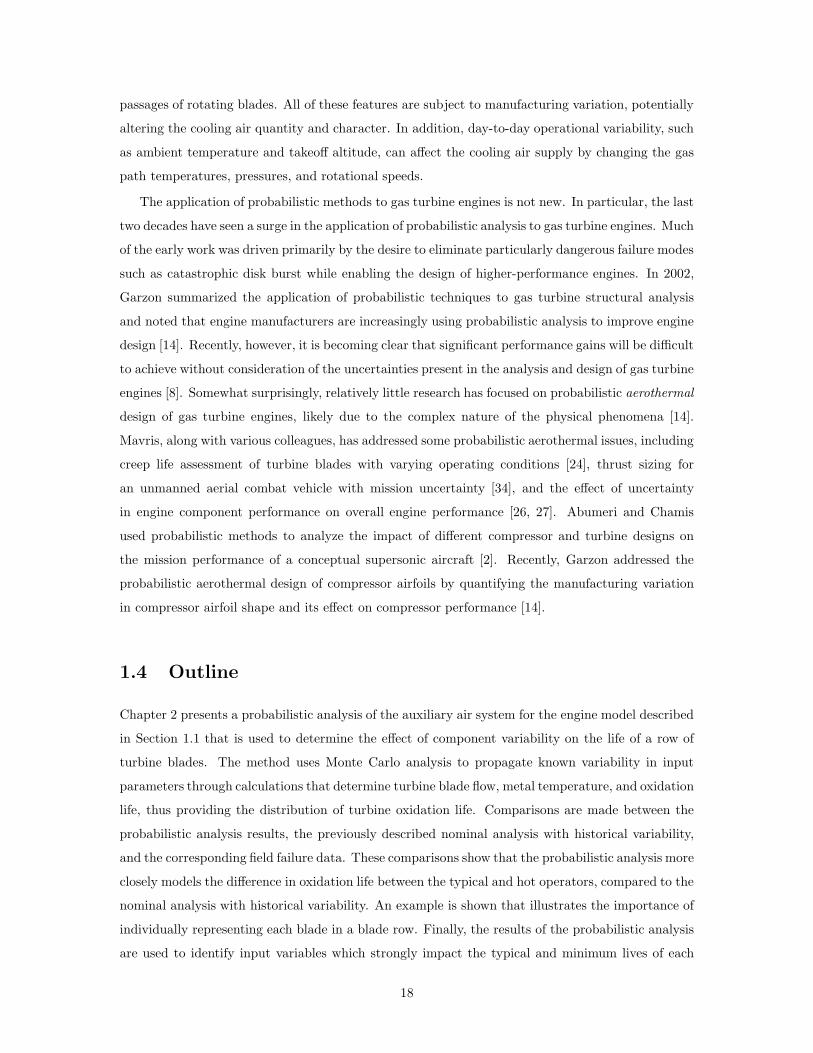
1.4 Outline

Chapter 2 presents a probabilistic analysis of the auxiliary air system for the engine model described

in Section 1.1 that is used to determine the effect of component variability on the life of a row of

turbine blades. The method uses Monte Carlo analysis to propagate known variability in input

parameters through calculations that determine turbine blade flow, metal temperature, and oxidation

life, thus providing the distribution of turbine oxidation life. Comparisons are made between the

probabilistic analysis results, the previously described nominal analysis with historical variability,

and the corresponding field failure data. These comparisons show that the probabilistic analysis more

closely models the difference in oxidation life between the typical and hot operators, compared to the

nominal analysis with historical variability. An example is shown that illustrates the importance of

individually representing each blade in a blade row. Finally, the results of the probabilistic analysis

are used to identify input variables which strongly impact the typical and minimum lives of each

18

fleet. For the engine model considered, the effective flow area of the leading-edge cooling passage is

the dominant source of variability.

Chapter 3 presents a simplified model of a blade cooling air supply system which enables iden-

tification of the dominant mechanisms affecting individual blade cooling flow, in particular blade-

to-blade variability and the relative sensitivities of the supply system and blade flows to changes

in blade plenum pressure. Based on these results, a method is proposed for selectively assembling

turbine blade sets by flow class that can decrease the impact of manufacturing variability on blade

temperature and life. The simplified model is extended to describe the behavior of blades with mul-

tiple cooling passages, specifically addressing the impact of inter-passage correlation on individual

blade flow. Chapter 3 also presents an estimate of the potential increase in the blades’ ability to

withstand increased turbine inlet temperature that can be achieved through selective assembly.

Chapter 4 considers the application of the selective assembly method to the first turbine rotor of

the commercial turbofan described in Chapter 2. The application uses probabilistic simulations of the

auxiliary air system of this turbofan to quantify the benefits of the selective assembly process on blade

flow, metal temperature, and engine life due to oxidation damage for a representative population of

blades. An example using a scheme based on three classes of blade coolant flow capability shows that

the lives of low-flow, nominal-flow, and high-flow blade classes can be increased 3%, 52%, and 106%,

respectively. Alternatively, selective assembly allows blades to withstand turbine inlet temperature

increases of 2◦F , 40◦F , and 79◦F , respectively.

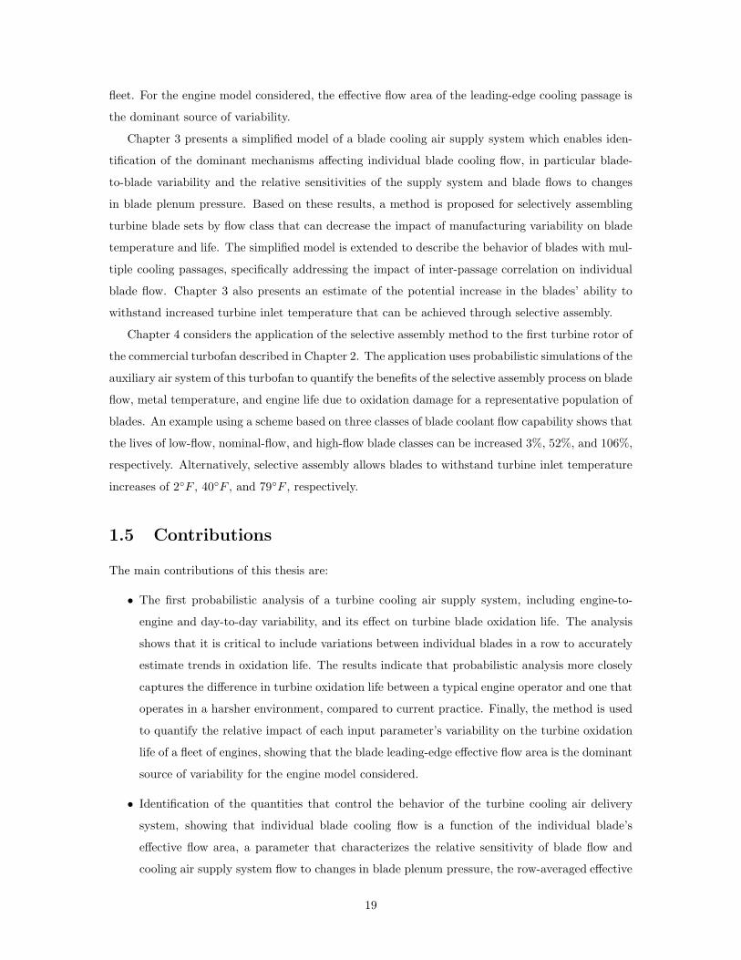
1.5 Contributions

The main contributions of this thesis are:

• The first probabilistic analysis of a turbine cooling air supply system, including engine-to-

engine and day-to-day variability, and its effect on turbine blade oxidation life. The analysis

shows that it is critical to include variations between individual blades in a row to accurately

estimate trends in oxidation life. The results indicate that probabilistic analysis more closely

captures the difference in turbine oxidation life between a typical engine operator and one that

operates in a harsher environment, compared to current practice. Finally, the method is used

to quantify the relative impact of each input parameter’s variability on the turbine oxidation

life of a fleet of engines, showing that the blade leading-edge effective flow area is the dominant

source of variability for the engine model considered.

• Identification of the quantities that control the behavior of the turbine cooling air delivery

system, showing that individual blade cooling flow is a function of the individual blade’s

effective flow area, a parameter that characterizes the relative sensitivity of blade flow and

cooling air supply system flow to changes in blade plenum pressure, the row-averaged effective

19

flow area of all the blades in a row, and the statistical correlation between multiple passages

within a single blade. Also, the explanation is extended to describe the effect of blades with

multiple cooling passages, particularly highlighting the effect of statistical correlation between

the flow capability of passages within a blade.

• A novel method of selectively assembling rows of turbine blades based on their blade cooling

flow capability that improves the turbine oxidation life of the majority of engines in a fleet of

a particular engine, while segregating the lowest-life blades into a set that is no worse than

current practice. Selective assembly can be used to increase turbine oxidation life, decrease

blade coolant flow requirements, or increase the turbine inlet temperature capability of the

blades. A numerical example shows that selective assembly can allow blades to withstand

increased turbine inlet temperatures equivalent to the turbine inlet temperature increases

observed over several years of engine development.

20

Chapter 2

Probabilistic Analysis of a Turbine

Cooling Air Delivery System

2.1 Introduction

This chapter presents a probabilistic analysis of the engine used by the operators described in Section

1.1 to quantify the variability in blade flow and oxidation life due to variability in ambient conditions,

main gaspath conditions, the cooling air delivery system, and the flow capability of the blade internal

cooling passages. A quasi-one-dimensional network flow model of the auxiliary air system for this

engine is used to calculate changes in the blade coolant flow due to the above variabilities. For this

analysis, the network flow model individually represents every first-stage turbine blade. Coolant

flow changes are used to calculate blade metal temperatures, which are used to calculate oxidation

lives. A Monte Carlo approach is used to propagate known variability in input parameters through

the analytical model to characterize the distributions of blade flow and turbine oxidation life.

The probabilistic analysis demonstrates that every blade in a turbine row must be individually

modeled in order to accurately estimate the distribution of blade flow (and therefore blade life)

for a population of jet engines. In particular, since the oxidation life of a blade row is limited

by the highest temperature (and therefore lowest-flowing) blades, every blade must be individually

represented to correctly model (1) the probability of observing (within a row) a blade with a low

coolant flow capability, and (2) the flow rate (and therefore the metal temperature and life) of these

passages.

Comparisons are made between the probabilistic model, the nominal analysis from Section 1.1,

and the corresponding field failure data. These comparisons show that the probabilistic analysis

more closely models the difference in oxidation life between the typical and hot operators.

Finally, the results of the probabilistic analysis are used to identify input variables whose variabil-

21

ity strongly impacts the typical and minimum lives of each fleet. For the engine model considered,

the effective flow area of the leading-edge cooling passage is the dominant source of variability.

2.2 Flow Network Analysis

This section describes the flow network modeling of an auxiliary air system and turbine blades.

While the description of the flow network is for a specific engine, flow network analysis is a widely-

used technique for modeling of auxiliary air systems. The auxiliary air system analyzed in this

thesis is from a high-bypass turbofan that powers a large, long-range commercial aircraft. The flow

network analysis estimates the temperature, pressure, and flow rates throughout the auxiliary air

system including the passages of the turbine blades.

Of particular interest for the present study is the turbine cooling air delivery system, which is

a portion of the entire auxiliary air system (Figure 2-1) [38]. The turbine cooling air originates

from the main gas path flow as it surrounds the combustion chamber (Station 1 in Figure 2-1).

This flow then enters a non-rotating tangential on-board injector (TOBI) (Station 2), which imparts

tangential swirl while directing the swirling flow towards holes in a rotating seal. The flow enters the

holes in the rotating seal (Station 3) then migrates radially toward the cavities below each turbine

blade (Station 4). The flow then proceeds into the turbine blade internal passages to convectively

cool the airfoil and continues out numerous small holes in the airfoil to provide a protective film of

cooler air [41, 38].

A flow network model is used to simulate the behavior of the entire auxiliary air system for this

engine model [4]. The model consists of many chambers that are interconnected by flow restrictions.

A variety of fluid dynamic components are used, such as sharp orifices, isentropic expansions and

contractions, free and forced vortices, and empirical correlations between mass flow and pressure

ratio. For this study 1037 restrictions and 483 chambers were used. An equilibrium solution is

found iteratively for temperature, pressure, and mass flow.

The network flow analysis makes the following assumptions:

• Simple fluid

• Steady state

• Internal flow

• Subsonic flow

• 1D flow

• Uniform flow

• 1 inlet surface and 1 exit surface for every restriction

• Constant enthalpy, velocity, and density over area

• Velocities normal to areas

• No heat interaction with surroundings

• No work interactions with surroundings

22

1 2 3

4

Rotating Structure

Static Structure

Cooling Air

Combustor

1st Stage Vane

1st Stage Blade

TOBI 1st StageTurbine Disk

Rotating Seal

Figure 2-1: Schematic cross section of area of interest, including the aft portion of the combustorand the first stage of the high-pressure turbine, where stations 1-4 indicate the turbine cooling airpath.

• Constant surface roughness and dynamic viscosity.

In addition, the network flow analysis assumes the following twelve variables are independent:

• Length

• Inlet hydraulic diameter

• Outlet hydraulic diameter

• Surface roughness

• Dynamic viscosity

• Inlet density

• Inlet velocity

• Radius of curvature

• Deflection angle

• Inlet area

• Specific heat at constant pressure

• Specific heat at constant volume.

23

The change in any dependent variable across a restriction (total pressure, for example) is a function

of the twelve independent variables. For chambers where the temperature and pressure are known,

these values are fixed at their known values. The remaining chambers are assigned estimated initial

values of temperature and pressure. Newton-Raphson iterations are performed that update unknown

pressures, temperatures, and flows until the flow network satisfies continuity and conservation of

energy [3].

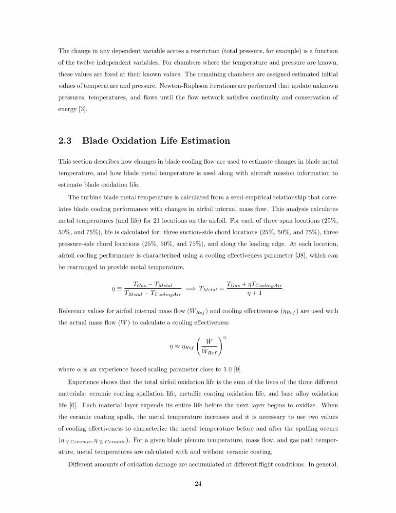
2.3 Blade Oxidation Life Estimation

This section describes how changes in blade cooling flow are used to estimate changes in blade metal

temperature, and how blade metal temperature is used along with aircraft mission information to

estimate blade oxidation life.

The turbine blade metal temperature is calculated from a semi-empirical relationship that corre-

lates blade cooling performance with changes in airfoil internal mass flow. This analysis calculates

metal temperatures (and life) for 21 locations on the airfoil. For each of three span locations (25%,

50%, and 75%), life is calculated for: three suction-side chord locations (25%, 50%, and 75%), three

pressure-side chord locations (25%, 50%, and 75%), and along the leading edge. At each location,

airfoil cooling performance is characterized using a cooling effectiveness parameter [38], which can

be rearranged to provide metal temperature,

η ≡TGas − TMetal

TMetal − TCoolingAir=⇒ TMetal =

TGas + ηTCoolingAir

η + 1.

Reference values for airfoil internal mass flow (WRef ) and cooling effectiveness (ηRef ) are used with

the actual mass flow (W ) to calculate a cooling effectiveness

η ≈ ηRef

(

W

WRef

)α

where α is an experience-based scaling parameter close to 1.0 [9].

Experience shows that the total airfoil oxidation life is the sum of the lives of the three different

materials: ceramic coating spallation life, metallic coating oxidation life, and base alloy oxidation

life [6]. Each material layer expends its entire life before the next layer begins to oxidize. When

the ceramic coating spalls, the metal temperature increases and it is necessary to use two values

of cooling effectiveness to characterize the metal temperature before and after the spalling occurs

(η w/ Ceramic, η w/o Ceramic). For a given blade plenum temperature, mass flow, and gas path temper-

ature, metal temperatures are calculated with and without ceramic coating.

Different amounts of oxidation damage are accumulated at different flight conditions. In general,

24

higher-thrust engine operation (e.g. takeoff) does more damage than lower-thrust (e.g. cruise). To

a lesser extent, the amount of time spent at a condition plays a role. To minimize the amount of

wear on an engine, airlines frequently takeoff at less than engine full-rated thrust capability. The

effects of engine operation at derated thrust settings are included in the lifing estimation described

below.

At full-rated takeoff conditions, the life is estimated for each material layer (ceramic coating,

metallic coating, and base alloy) using proprietary, specimen-based empirical relationships between

metal temperature and typical (cumulative probability of 50%) time to failure. These relationships

take the form [36, 35],

L T/O :Full = C1eC2(TMetal−C3) (2.1)

where C1, C2, and C3 are empirical constants. For each layer, the full-rated takeoff damage per

cycle is

D T/O :Full =t T/O

L T/O :Full

where t T/O is the time spent at the takeoff condition during a single mission.

This engine typically operates at 10% and 20% derated thrust when full-rated thrust is not

required (when lightly loaded, for example). The damage at the derated takeoff thrust is based on

a scaling of the full-rated takeoff thrust:

D T/O :10%Derate = D T/O :Full × SF10%

D T/O :20%Derate = D T/O :Full × SF20%

where SF10% and SF20% are the scale factors. These scale factors are derived from a higher-fidelity

lifing analysis (performed during the design of this engine [9]) at the different thrust settings:

SF10% ≡

[

D T/O :10%Derate

D T/O :Full

]High Fidelity

SF20% ≡

[

D T/O :20%Derate

D T/O :Full

]High Fidelity

.

Using scale factors to account for derated operation greatly simplifies the application of probabilistic

analysis. The damage at each takeoff setting is combined through a weighted sum,

DEqv. T/O = D T/O:Full × wFull + D T/O :10%Derate × w10% + D T/O :20%Derate × w20%

where the weights reflect the percentage of flights at each takeoff thrust setting (wFull, w10%, w20%).

Takeoff causes the majority of oxidation damage, which is calculated with this analysis. The

remainder of the flight also causes oxidation damage which is not calculated in this analysis. This

25

damage is included as an additional constant amount of damage. In this example, the non-takeoff

portion of the mission accounts for less than 20% of the total damage. The damage accumulated

during the remainder of the flight (DNonT/O ) is also available from the higher-fidelity lifing analysis

[9] and is added to the equivalent takeoff damage value to arrive at an equivalent mission damage

DEqv. Mission = DEqv. T/O + DNonT/O .

As a result, the non-takeoff damage does not include the effects of engine-to-engine variability.

The calculated life to failure for each material layer is the actual flight length (in hours per flight,

tMission) divided by the equivalent total damage per flight

Lsingle material layer =tMission

DEqv. Mission.

Each material layer begins to oxidize only when exposed, so the total oxidation life of a blade is the

sum of the oxidation lives of the individual material layers

LBlade = LCeramic Coating + LMetallic Coating + LBase Alloy. (2.2)

The different material layers account for roughly 10%, 70%, and 20% of a blade’s life, respectively.

Because the focus of this study is to characterize the variability in unscheduled engine removals due

to turbine-blade-related oxidation, the blade with the lowest oxidation life in the entire blade row

defines that particular engine’s oxidation life

LBlade Row = mini=1...n

(LBlade,i)

where n is the number of blades in a blade row.

2.4 Probabilistic Analysis

Two distinctly different types of input variability arise in this application: day-to-day and engine-

to-engine. Engine deterioration effects (non-random) are included within the nominal network flow

model used for this analysis, including seal deterioration within the turbine cooling air delivery

system [9, 29].

Each airline’s aircraft experience different ambient temperatures as a function of geographical

location, time of day, season, etc. It is customary to characterize the ambient temperature environ-

ment by a distribution of the difference between the actual ambient temperature and the temperature

of a standard day (referred to as ∆TAmbient), where TStandardDay = 59◦F . Airline A operates this

particular fleet of engines at a mean ∆TAmbient of 1◦F with a standard deviation of 18◦F [9]. Airline

26

B operates between locations with higher ambient temperatures, at a mean ∆TAmbient of 14◦F with

a standard deviation of 18◦F [9].

A methodology used to account for day-to-day variability is adapted from current design practice

[11]. The variety of ambient temperatures experienced by an airline is characterized by a normal

probability distribution. To calculate the life for a given engine, the probability density function

of ambient temperature is segmented into ten discrete sections, each representing equal probability.

Each ambient temperature value is used to determine the appropriate engine cycle temperatures,

pressures, flows, and rotational speeds which are interpolated from tables of engine performance at

different ambient temperatures [9]. The oxidation damage calculations are carried out at the center

of each discrete section of the ambient temperature distribution, then summed (each with a weight

of 1/10) to calculate the average damage, including ambient temperature variability, over the life of

a particular engine.

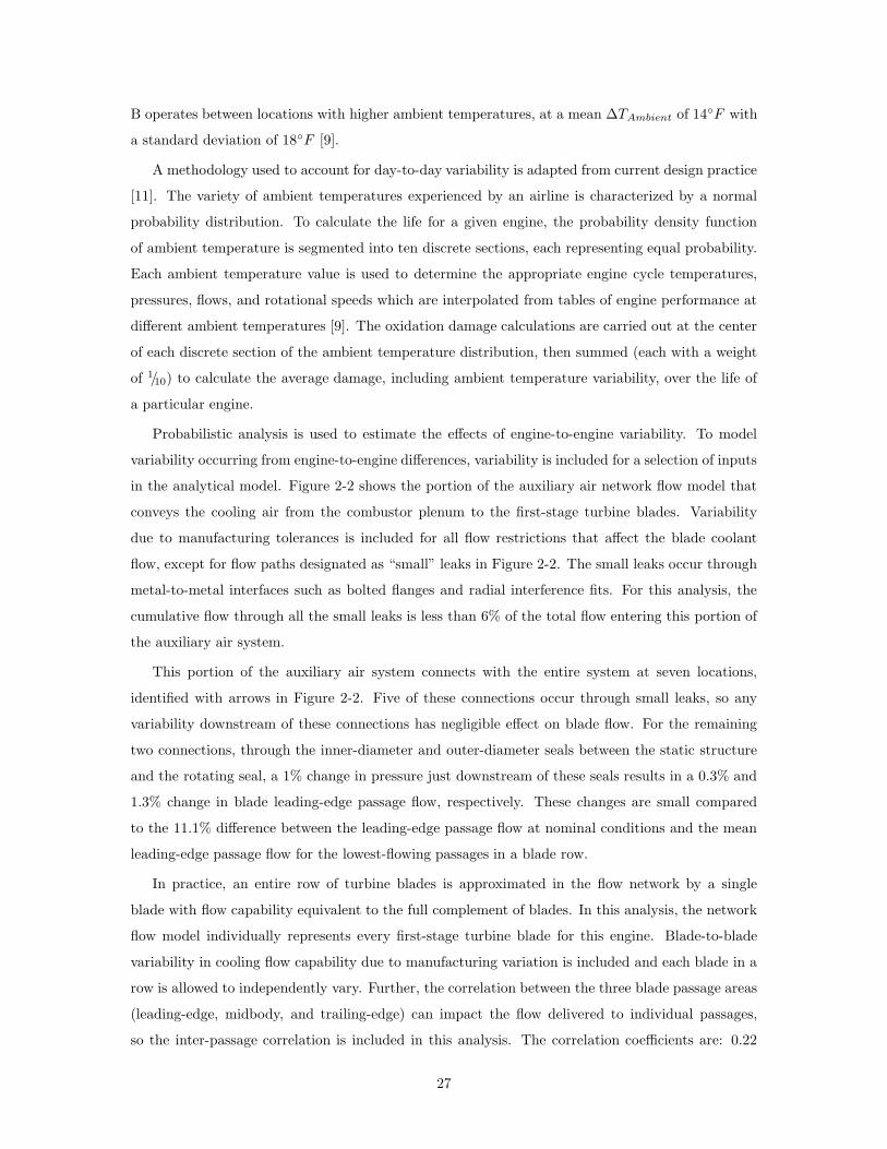
Probabilistic analysis is used to estimate the effects of engine-to-engine variability. To model

variability occurring from engine-to-engine differences, variability is included for a selection of inputs

in the analytical model. Figure 2-2 shows the portion of the auxiliary air network flow model that

conveys the cooling air from the combustor plenum to the first-stage turbine blades. Variability

due to manufacturing tolerances is included for all flow restrictions that affect the blade coolant

flow, except for flow paths designated as “small” leaks in Figure 2-2. The small leaks occur through

metal-to-metal interfaces such as bolted flanges and radial interference fits. For this analysis, the

cumulative flow through all the small leaks is less than 6% of the total flow entering this portion of

the auxiliary air system.

This portion of the auxiliary air system connects with the entire system at seven locations,

identified with arrows in Figure 2-2. Five of these connections occur through small leaks, so any

variability downstream of these connections has negligible effect on blade flow. For the remaining

two connections, through the inner-diameter and outer-diameter seals between the static structure

and the rotating seal, a 1% change in pressure just downstream of these seals results in a 0.3% and

1.3% change in blade leading-edge passage flow, respectively. These changes are small compared

to the 11.1% difference between the leading-edge passage flow at nominal conditions and the mean

leading-edge passage flow for the lowest-flowing passages in a blade row.

In practice, an entire row of turbine blades is approximated in the flow network by a single

blade with flow capability equivalent to the full complement of blades. In this analysis, the network

flow model individually represents every first-stage turbine blade for this engine. Blade-to-blade

variability in cooling flow capability due to manufacturing variation is included and each blade in a

row is allowed to independently vary. Further, the correlation between the three blade passage areas

(leading-edge, midbody, and trailing-edge) can impact the flow delivered to individual passages,

so the inter-passage correlation is included in this analysis. The correlation coefficients are: 0.22

27

Figure 2-2: Schematic cross section of area of interest, including the aft portion of the combustorand the first stage of the high-pressure turbine, showing a portion of network flow model.

between the leading-edge and midbody passages, 0.08 between the leading-edge and trailing-edge

passages, and 0.25 between the midbody and trailing-edge passages. Chapter 3 will discuss the effect

of inter-passage correlation.

The following geometric parameters are treated as randomly varying:

1. TOBI Radius from Centerline

2. Rotating Seal Hole Radius from Centerline

3. ID TOBI Seal Radius

4. OD TOBI Seal Radius

5. Rotating Seal Hole Area

6. ID TOBI Seal Discharge Coefficient

7. OD TOBI Seal Discharge Coefficient

8. TOBI Discharge Coefficient

9. Blade Leading Edge Passage Effective Area

10. Blade Midbody Passage Effective Area

28

11. Blade Trailing Edge Passage Effective Area

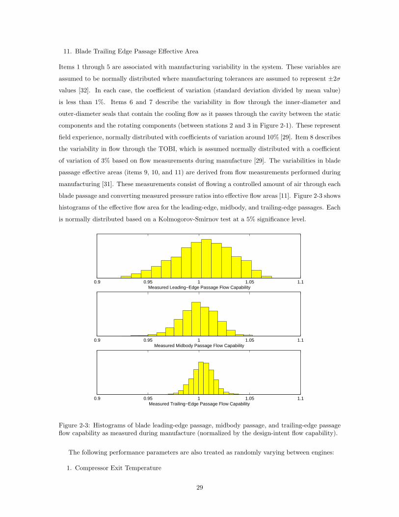
Items 1 through 5 are associated with manufacturing variability in the system. These variables are

assumed to be normally distributed where manufacturing tolerances are assumed to represent ±2σ

values [32]. In each case, the coefficient of variation (standard deviation divided by mean value)

is less than 1%. Items 6 and 7 describe the variability in flow through the inner-diameter and

outer-diameter seals that contain the cooling flow as it passes through the cavity between the static

components and the rotating components (between stations 2 and 3 in Figure 2-1). These represent

field experience, normally distributed with coefficients of variation around 10% [29]. Item 8 describes

the variability in flow through the TOBI, which is assumed normally distributed with a coefficient

of variation of 3% based on flow measurements during manufacture [29]. The variabilities in blade

passage effective areas (items 9, 10, and 11) are derived from flow measurements performed during

manufacturing [31]. These measurements consist of flowing a controlled amount of air through each

blade passage and converting measured pressure ratios into effective flow areas [11]. Figure 2-3 shows

histograms of the effective flow area for the leading-edge, midbody, and trailing-edge passages. Each

is normally distributed based on a Kolmogorov-Smirnov test at a 5% significance level.

0.9 0.95 1 1.05 1.1Measured Leading−Edge Passage Flow Capability

0.9 0.95 1 1.05 1.1Measured Midbody Passage Flow Capability

0.9 0.95 1 1.05 1.1Measured Trailing−Edge Passage Flow Capability

Figure 2-3: Histograms of blade leading-edge passage, midbody passage, and trailing-edge passageflow capability as measured during manufacture (normalized by the design-intent flow capability).

The following performance parameters are also treated as randomly varying between engines:

1. Compressor Exit Temperature

29

2. High-Pressure Turbine Inlet Temperature

3. High-Pressure Turbine Exit Temperature

4. Low-Pressure Turbine Exit Temperature

5. Low-Pressure Spool Rotational Speed

6. High-Pressure Spool Rotational Speed

Items 1-6 describe engine-to-engine variabilities in cycle parameters superimposed on the cycle pa-

rameters selected via the ambient temperature. The selection of variable performance parameters

and their magnitude is based on field experience [9]. Although it is possible that correlation exists

between these variables, these quantities are treated as independent, in accordance with standard

practice.

Variability within the spallation life due to the scatter of specimen lives used to generate the

spallation lifing estimate is also included [10]. The spallation life variability is applied to the ceramic

coating life prior to the summation shown in Equation (2.2).

The probabilistic calculations are performed for each airline’s fleet of engines. In each case, 1000

Monte Carlo simulations are performed. Each simulation represents a single engine, which is an

instance of the randomly selected engine-to-engine variable parameters. Each simulated engine ex-

periences the entire distribution of day-to-day ambient temperature variability (as described above),

where engine temperatures, pressures, flows, and rotational speeds are determined by correlations

of engine performance with ambient temperature [9]. Blade life is calculated for 21 locations on the

airfoil using the procedure in Section 2.2, where the weighted summation of oxidation damage at

each ambient temperature is performed after the application of Equation (2.2). The minimum life

location on each blade is selected, then from this the minimum life blade is selected from the blade

row of interest to represent the engine’s life due to turbine blade oxidation. The Monte Carlo results

show that minimum-life always occurs at the same location which is cooled by the leading-edge

passage flow. The location of minimum-life is consistent with field experience for this blade [10].

2.5 Probabilistic Analysis Results

The inclusion of all the blades within a row leads to different behavior of the flow network, resulting

in different blade cooling flow. With all blades included, the flow capability of a given blade has the

freedom to vary in accordance with the previously identified input variabilities and correlations. An

individual blade’s cooling flow is thus influenced by the flow characteristics of the remaining blades.

Chapter 3 will focus on how variability in effective flow area impacts the coolant flow delivered to

each individual blade.

The top portion of Figure 2-4 shows histograms of blade leading-edge cooling flow for all the

blades in every row for Airline A and Airline B. The nominal blade leading-edge passage flows are

included for Airline A (dashed line) and Airline B (dash-dot line). For both airlines, the probabilistic

30

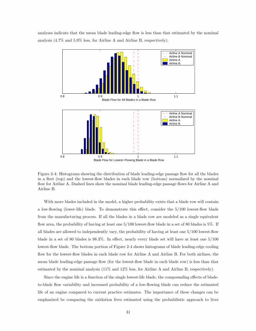
analyses indicate that the mean blade leading-edge flow is less than that estimated by the nominal

analysis (4.7% and 5.9% less, for Airline A and Airline B, respectively).

0.8 0.9 1 1.1Blade Flow for All Blades in a Blade Row

Airline A NominalAirline B NominalAirline AAirline B

0.8 0.9 1 1.1Blade Flow for Lowest−Flowing Blade in a Blade Row

Airline A NominalAirline B NominalAirline AAirline B

Figure 2-4: Histograms showing the distribution of blade leading-edge passage flow for all the bladesin a fleet (top) and the lowest-flow blades in each blade row (bottom) normalized by the nominalflow for Airline A. Dashed lines show the nominal blade leading-edge passage flows for Airline A andAirline B.

With more blades included in the model, a higher probability exists that a blade row will contain

a low-flowing (lower-life) blade. To demonstrate this effect, consider the 5/100 lowest-flow blade

from the manufacturing process. If all the blades in a blade row are modeled as a single equivalent

flow area, the probability of having at least one 5/100 lowest-flow blade in a set of 80 blades is 5%. If

all blades are allowed to independently vary, the probability of having at least one 5/100 lowest-flow

blade in a set of 80 blades is 98.3%. In effect, nearly every blade set will have at least one 5/100

lowest-flow blade. The bottom portion of Figure 2-4 shows histograms of blade leading-edge cooling

flow for the lowest-flow blades in each blade row for Airline A and Airline B. For both airlines, the

mean blade leading-edge passage flow (for the lowest-flow blade in each blade row) is less than that

estimated by the nominal analysis (11% and 12% less, for Airline A and Airline B, respectively).

Since the engine life is a function of the single lowest-life blade, the compounding effects of blade-

to-blade flow variability and increased probability of a low-flowing blade can reduce the estimated

life of an engine compared to current practice estimates. The importance of these changes can be

emphasized be comparing the oxidation lives estimated using the probabilistic approach to lives

31

estimated using the nominal approach. Histograms of the oxidation lives from the probabilistic

analyses are shown in the bottom graph of Figure 2-5 for Airline A and Airline B. This figure also

includes probability density functions representing the field failure data for both airlines (top graph)

and the nominal analysis with historical variability (middle graph) described in Section 1.1. The

field data are fit with Weibull probability density functions using maximum likelihood analysis of

multiply censored data (i.e. non-failures) [1, 30].

Both the nominal analysis and the probabilistic analysis capture the trend that Airline B engines

fail earlier than Airline A engines, largely due to the difference in ambient temperature. However, by

capturing the effects of variability on blade cooling flow, the probabilistic analysis more accurately

models the large relative difference in life between Airline A and Airline B. The field data show a

77% (62% to 84% with 95% confidence) reduction in mean life between Airline A and Airline B. The

probabilistic analyses show a 72% (71% to 74% with 95% confidence) decrease, while the nominal

analyses with historical variability show only a 56% decrease.

0 0.18 0.76 1 2

Airline A Field DataAirline B Field Data

0 0.39 0.9 1 2

Airline A NominalAirline B Nominal

0 0.13 0.45 1 2Reference Life

Airline A ProbabilisticAirline B Probabilistic

Figure 2-5: Probability density functions comparing Airline A and Airline B for: (1) field failuredata, (2) nominal analyses with historical variability, and (3) probabilistic analyses. Mean valuesare represented by dotted lines.

Hypothesis testing can be used to quantitatively compare the probabilistic results to the field

failure data. To avoid introducing additional uncertainty, a methodology is used that does not assign

probability distributions to the field data. Using Airline A as an example, consider a null hypothesis

that the probabilistic results and the field data represent the same distribution. This leaves the

32

alternate hypothesis that the two data sets represent different distributions. The test statistic is

taken to be the number of failed engines, given a fleet of engines that exist at the lives shown in

Figure 1-3 in Section 1.1. The probability of failure of each engine in the Airline A fleet is taken

from an empirical cumulative distribution function of the Monte Carlo results. A random process

is created that simulates 10,000 fleets with each engine in each fleet having a random probability

(uniformly distributed between zero and one) assigned to it. Each engine in each random process

fleet is compared to its respective probability of failure and is deemed either a failure or non-failure.

This simulation of 10,000 fleets determines the probability of n failures occurring for this fleet (where

n is a number of failed engines). This distribution is shown in the top left of Figure 2-6 for Airline

A. The probability of seeing two failures (as seen in the field data), using the individual probabilities

of failure from the probabilistic analysis is 9% (i.e. 900 occurrences of two failures in 10,000 fleets).

Since this probability is not less than a significance level of 5%, the null hypothesis is not rejected,

which is evidence for the conclusion that the field failure distribution and the probabilistic analysis

results share the same distribution.

The same analysis is also used to compare the probabilistic results to the field data for Airline

B. The top right histogram in Figure 2-6 shows the distribution of the number of failures, given

the existing fleet of engine lives shown in Figure 1-3 in Section 1.1. In this case, the probability of

seeing six failures (as seen in the field data), using the individual probabilities of failure from the

probabilistic analysis is less than 1%, which is small enough to warrant rejection of the null hypoth-

esis. Therefore, the probabilistic results and the field data do not represent the same distribution

for Airline B.

The hypothesis testing methodology is also used to compare the nominal analyses with historical

variability and the field failure distributions. The bottom left histogram in Figure 2-6 shows that

the probability of two failures using the nominal failure distribution, given the existing Airline A

fleet, is 6%. For Airline B, the bottom right histogram in Figure 2-6 shows that the probability

of six failures is 0%, which indicates that the nominal analysis does not match the Airline B field

failure distribution.

The probabilistic analysis and the nominal analysis show similar results for Airline A. For Airline

B, however, the probabilistic analysis estimates the fleet should have experienced about nine failures,

while the nominal analysis estimates the fleet should have experienced zero failures. Airline B

actually experienced six failures, so the probabilistic analysis provides a better estimate than the

nominal analysis.

A potential source of the discrepancy between the probabilistic analysis and the field data may lie

in the experience-based scaling factors used to determine oxidation life from blade metal temperature

(Equation 2.1). Typically, these scaling factors are used so that a deterministically predicted nominal

life matches the mean life demonstrated in the field. In many cases, however, the response is such

33

0 2 4 6 8 100

0.2

0.4

0.6

0.8

Number of Failures

Pro

babi

lity

Airline B: Probabilistic

0 2 4 6 8 100

0.2

0.4

0.6

Number of Failures

Pro

babi

lity

Airline A: Probabilistic

0 2 4 6 8 100

0.2

0.4

0.6

0.8

Number of Failures

Pro

babi

lity

Airline B: Nominal

0 2 4 6 8 100

0.2

0.4

0.6

Number of Failures

Pro

babi

lity

Airline A: Nominal

Figure 2-6: Results of hypothesis tests comparing field data to probabilistic analyses and nominalanalyses for Airline A and Airline B. Each graph shows the probabilities of experiencing differentnumbers of failed engines, given the existing airline fleet, assuming the particular analysis is correct.Dashed lines indicate the number of failures seen in the field data.

that the nominal response is different from the mean response. In effect, this scaling methodology

lumps together any differences between the laboratory and the field with the shift from the nominal

life to the statistical mean life. When scaling factors such as these are used within a probabilistic

analysis, which automatically accounts for the nominal-to-mean shift, then the nominal-to-mean

shift effect is included twice. Further work is needed to identify and remove historical factors from

the life estimation methods to allow the probabilistic analysis to more accurately model the field

experience.

The above analysis assumes that the single lowest-life blade dictates the oxidation life of the

engine. It is possible that engine oxidation life is associated with several low-life blades, instead of

the single lowest-life blade. For example, with infrequent inspections, it is possible that an inspection

finds several blades that have enough damage to warrant removal of the engine for overhaul. Thus,

the distributions of engine oxidation life are dependent on the number of oxidized blades needed to

establish a blade row failure. Figure 2-7 shows the dependence of mean blade row reference life and

B5 (time to 5% failing) blade row reference life on the number of failed blades required for a blade

row failure for both airlines. The lives shown for one blade failure correspond to the probabilistic

analysis distributions in Figure 2-5. For both airlines, the mean and B5 failure lives increase with

34

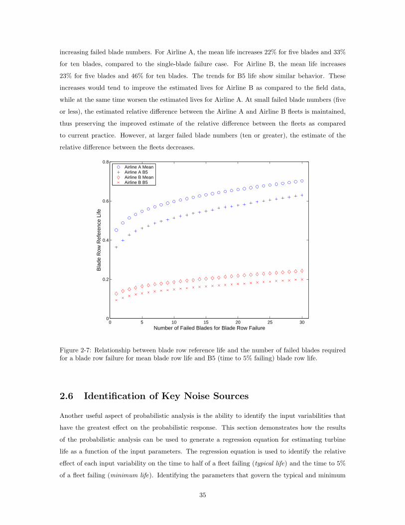
increasing failed blade numbers. For Airline A, the mean life increases 22% for five blades and 33%

for ten blades, compared to the single-blade failure case. For Airline B, the mean life increases

23% for five blades and 46% for ten blades. The trends for B5 life show similar behavior. These

increases would tend to improve the estimated lives for Airline B as compared to the field data,

while at the same time worsen the estimated lives for Airline A. At small failed blade numbers (five

or less), the estimated relative difference between the Airline A and Airline B fleets is maintained,

thus preserving the improved estimate of the relative difference between the fleets as compared

to current practice. However, at larger failed blade numbers (ten or greater), the estimate of the

relative difference between the fleets decreases.

0 5 10 15 20 25 300

0.2

0.4

0.6

0.8

Number of Failed Blades for Blade Row Failure

Bla

de R

ow R

efer

ence

Life

Airline A MeanAirline A B5Airline B MeanAirline B B5

Figure 2-7: Relationship between blade row reference life and the number of failed blades requiredfor a blade row failure for mean blade row life and B5 (time to 5% failing) blade row life.

2.6 Identification of Key Noise Sources

Another useful aspect of probabilistic analysis is the ability to identify the input variabilities that

have the greatest effect on the probabilistic response. This section demonstrates how the results

of the probabilistic analysis can be used to generate a regression equation for estimating turbine

life as a function of the input parameters. The regression equation is used to identify the relative

effect of each input variability on the time to half of a fleet failing (typical life) and the time to 5%

of a fleet failing (minimum life). Identifying the parameters that govern the typical and minimum

35

oxidation failure lives can suggest tolerance management practices to increase the failure life of a

fleet of engines. In some cases, it may be difficult to reduce the variability of a parameter and the

identification of the key parameters indicates which aspects of the problem could benefit from further

investigation, potentially including identifying designs that are insensitive to these variabilities.

For this study, regression analysis is used to determine the coefficients of a polynomial that

provide the best fit to the Monte Carlo data in a least-squares sense [7]. The polynomial consists

of linear and squared terms only, as there are too many interactions (e.g. x1x2) to compute. Thus,

the regression equation has the form

Life ≈ a +n∑

i=1

bixi +n∑

i=1

cix2i

where xi represents the input parameters (i = 1...n) and a, bi, and ci represent the regression

coefficients. For this example, n = 261 because each blade’s passages are individually included.

Since the input parameters vary widely in magnitude, the regression is performed on input

parameters that have been transformed into standard normal variates, to highlight the relative

effect of each input’s variability. This transformation is given by

z1 =xi − µi

σi

where µi is the mean of the input parameter and σi is its standard deviation. To perform the

regression, the input parameters (i = 1...n) for every Monte Carlo iteration (j = 1...m) used in the

probabilistic analysis undergo the standard normal transformation and are placed into a matrix that

has the form (where zi,j represents input parameter i in Monte Carlo iteration j)

Z =

1 z1,1 . . . zn,1 z21,1 . . . z2

n,1

1 z1,2 . . . zn,2 z21,2 . . . z2

n,2

......

...

1 z1,m . . . zn,m z21,m . . . z2

n,m

.

The life calculated for each Monte Carlo iteration is placed into a vector

Y =

Life1

Life2

...

Lifem

.

36

The regression coefficients are obtained by [7]

B = (Z′Z)−1Z′Y

where

B =

a

b1

...

bn

c1

...

cn

.

For both airline cases, the R2 value for the least-squares fit is near 90%, which suggests that the

regression accounts for all but 10% of the response of oxidation life to the input variables.

The regression model allows for inexpensive evaluations of turbine oxidation life as a function

of the input parameters. An important use is to identify input parameters whose variability has

a large effect on the turbine oxidation life. These parameters would be candidates for improved

manufacturing processes or tighter allowable tolerances. To demonstrate the benefit of reduced

input parameter variability in a meaningful way, a reduction in variability of 10% of a parameter’s

standard deviation is used to compare the effects of each parameter. A Monte Carlo analysis of the

regression equation is performed separately for each input variable, where that variable’s standard

deviation has been reduced by 10% to simulate a decrease in the input’s variability (all other variables

retain their original variability).

Input variability can affect both the mean and variability of turbine oxidation life. To present the

combined effects of changes in the mean and variability of turbine oxidation life, results are presented

as changes to typical life (50% failed) and minimum life (5% failed). The top row in Figure 2-8 shows

changes in typical life for Airlines A and B due to a 10% reduction in the standard deviation of

each input parameter, with each input parameter considered separately. For both airlines, a 10%

reduction in the variability for input variable #9 (blade leading-edge effective area) has the largest

effect on typical life. Airline B, in particular, shows a 17% increase in mean life due to a 10%

decrease in the variability of blade leading-edge effective area.

The overhaul interval for a fleet of engines is intended to minimize the possibility of unscheduled

engine removals. The occurrence of unscheduled engine removals is dictated by the minimum life

of a fleet of engines. The bottom row of Figure 2-8 shows the change in minimum oxidation life

that results from a 10% decrease in each variable’s standard deviation. As before, the variability in

the blade leading edge effective area (Input Variable #9) has the largest impact on the minimum

37

life. Airline B’s minimum life increases 33% for a 10% decrease in blade leading edge area standard

deviation.

The regression analysis can also identify those input variables whose variability has little effect

on the typical and minimum oxidation lives. For these variables, it is possible to increase their

variability without significant effect on oxidation life. For example, the variability in the blade

midbody effective flow area for Airline B (Input Variable #10 in Figure 2-8) has little effect and

greater variability could be allowed for these insensitive variables.

2.7 Summary

This chapter presented a probabilistic methodology to determine the effect of component variability

on the cooling flow and oxidation life of a row of turbine blades. The method used a Monte Carlo

approach to propagate known variability in input parameters through an analysis to characterize

the distribution of turbine oxidation life.

The probabilistic analysis showed that it is critical that the network flow model individually

represent every blade in a blade row to accurately estimate individual blade flow and therefore

blade-row oxidation life. Including every blade individually increases the probability of observing

a low-flow (low-life) blade within a blade row. Further, all blades must be allowed to individually

vary to capture the correct behavior of the cooling air delivery system, and thus accurately estimate

blade metal temperature and life.

A distribution of the probability of oxidation failure was generated for each of two airlines. The

probabilistic distributions of failure times were compared to the field failure distributions of two

airlines and were shown to better capture the difference between a typical engine fleet and a fleet

operating in a hotter environment as compared to current practice.

Using regression analysis, the results of Monte Carlo analysis were used to establish the relative

effect of each input parameter’s variability on the distribution of turbine oxidation life, specifically

identifying which input variabilities drive turbine life. For both airlines, a 10% decrease in the

variability of blade leading edge effective flow area can have an impact on both the typical and

minimum life. For Airline B, this variability decrease can increase the minimum oxidation life of the

engine model by 33%.

38

0 5 10 15 200

0.2

0.4

0.6

Input Variable

Ref

eren

ce L

ife

Airline A

Typical LifeReduced Variability

0 5 10 15 200

0.2

0.4

0.6

Input Variable

Ref

eren

ce L

ife

Airline A

Minimum LifeReduced Variability

0 5 10 15 200

0.05

0.1

0.15

Input VariableR

efer

ence

Life

Airline B

Typical LifeReduced Variability

0 5 10 15 200

0.05

0.1

0.15

Input Variable

Ref

eren

ce L

ife

Airline B

Minimum LifeReduced Variability

Leading−EdgeArea

Figure 2-8: Changes in typical and minimum life that result from a 10% decrease in each variable’sstandard deviation superimposed on typical and minimum life, respectively (each variable consideredseparately) for Airline A and Airline B. Variables are: (1) TOBI radius, (2) rotating seal holelocation, (3) ID TOBI seal radius, (4) OD TOBI seal radius, (5) rotating seal hole area, (6) ID TOBIseal discharge coefficient, (7) OD TOBI seal discharge coefficient, (8) TOBI discharge coefficient, (9)blade leading-edge passage area, (10) blade midbody passage area, (11) blade trailing-edge passagearea, (12) HPC exit temperature, (13) HPT inlet temperature, (14) HPT exit temperature, (15)LPT exit temperature, (16) low-pressure spool rotational speed, (17) high-pressure spool rotationalspeed, and (18) ceramic coating spallation life.

39

Chapter 3

Behavior of Cooling Air Supply

Systems Including Blade Flow

Variability

3.1 Introduction

For the engine considered in Chapter 2, manufacturing variability in blade effective flow area was

shown to be the dominant driver for oxidation-related turbine blade failures. This chapter develops

an overall understanding of how the variability in blade effective area impacts the amount of coolant

flow delivered to each individual blade. Finally, this chapter presents the potential increase in turbine

inlet temperature that can be achieved through selective assembly.

This chapter begins by describing a network-flow model that highlights the behavior of the

cooling air supply system and a row of single-passage cooled turbine blades. This model simplifies

the network flow model from Chapter 2, only including an element representing the cooling air

supply system connected to a parallel set of elements representing each individual turbine blade. The

governing equations are linearized, in order to identify the controlling parameters of the system. The

linearized equations show that perturbations in blade plenum pressure and total system mass flow

are controlled by the row-average blade effective area perturbation and a parameter that represents

the relative sensitivities of flow upstream and downstream of the blade plenum to changes in blade

plenum pressure. Blade plenum pressure perturbation is shown to increase with decreased row-

average effective area, providing compensation for a set of blades that are on average low-flowing.

Finally, the flow in each individual blade is controlled by a combination of its individual effective

area perturbation, the row-average effective area perturbation, and the parameter that represents

41

the relative sensitivities of flow upstream and downstream of the blade plenum to changes in blade

plenum pressure .

A selective assembly method is proposed that decreases the impact of blade passage manufac-

turing variability on the life of a row of cooled turbine blades. The method classifies turbine blades

into groups based on the effective flow areas of the blade passages, then a row of blades is assembled

exclusively from blades of a single group1. A classification is considered in which blades are divided

into low-flow, nominal-flow, and high-flow groups. This selective assembly method will reduce the

blade-to-blade flow variability in a row and could result in increased certainty when estimating the

life of a blade due to temperature-induced failures. In particular, the life of a nominal-flow or high-

flow row will be increased (relative to a randomly-assembled row) since the life-limiting low-flow

blades would not be included in these higher-flowing rows. However, an additional important effect

occurs with respect to the individual blade flows in the classed assemblies. For rows assembled from

the low-flow class, the blade plenum pressure will tend to rise and the individual blade flows will be

closer to the design intent than for a single low-flow blade in a randomly-assembled row. Since the

blade metal temperature is strongly dependent on the blade flow, selective assembly can lower the

metal temperature of the lowest-flowing blades and increase the life of a turbine row beyond what

is possible from a randomly-assembled row.

In practice, most high-performance turbine blades have multiple cooling passages per blade.

To properly characterize the flow behavior of individual blades, it is necessary to account for the

statistical correlation (or lack thereof) between the effective areas of each passage in a blade. This

chapter thus includes an extension of the model to two passages per blade. A high level of inter-

passage correlation is found to maximize the benefit of selective assembly to individual blade flow.

While the selective assembly method can be used to increase life, an alternative use would be

to allow blades to withstand increased turbine inlet temperature while maintaining blade life (or

equivalently, blade metal temperature). The potential increases in turbine inlet temperature due

to selective assembly are thus quantified, including the effects of relative upstream and downstream

sensitivity to blade plenum pressure and inter-passage correlation.

3.2 Simplified Model of a Flow System with Single-Passage

Blades

The following sections describe a simplified model of a cooling supply system with a parallel set of

blades, shown in Figure 3-1, to qualitatively explain how the flow through an individual blade is

affected by (1) blade-to-blade variability in flow capability, (2) the relative sensitivity of the flow

1A patent application for this selective assembly methodology has been submitted to the United States Patent andTrademark Office with Serial Number 10/717408.

42

rate

inth

esu

pply

system

and

the

bla

des

toplen

um

pressu

repertu

rbatio

ns,

and

(3)

the

pro

posed

selective

assem

bly

pro

cess.In

this

simplifi

edm

odel

of

atu

rbin

erow

with

multip

leco

oled

bla

des,

Ps

As fs (P

s ,Pp )

Pg

Pp

A1 fb (P

p ,Pg )

m �1

m �im �

nm �

…

Ai fb (P

p ,Pg )

An fb (P

p ,Pg )

…

Fig

ure

3-1

:Sim

plifi

edm

odel

ofa

turb

ine

coolin

gair

supply

system

and

arow

ofn

cooled

turb

ine

bla

des.

As f

s (Ps ,P

p )rep

resents

the

coolin

gair

supply

system

and

Ai f

b (Pp ,P

g )rep

resents

each

cooled

bla

de.

the

coolin

gair

deliv

erysu

bsy

stemis

represen

tedby

the

effectiv

earea

,A

s ,and

am

ass

flow

-pressu

re

relatio

nsh

ip,f

s (Ps ,P

p ).E

ach

ofth

en

cooled

bla

des

isrep

resented

by

an

indiv

idualeff

ective

area

,

Ai ,

and

am

ass

flow

-pressu

rerela

tionsh

ip,f

b (Pp ,P

g ).T

he

gov

ernin

geq

uatio

ns

for

the

system

can

be

written

as:

m=

As f

s (Ps ,P

p )

mi

=A

i fb (P

p ,Pg )

i=

1,2

,...,n

m=

n∑i=

1

mi .

For

the

situatio

nin

which

all

bla

des

are

at

their

nom

inaleff

ective

area

s(A

i=

An

om

for

all

i,

where

An

om

isth

enom

inaleff

ective

area

),defi

ne

the

nom

inalbla

de

mass

flow

as

mn

om

≡1n

m.

Consid

erth

ebeh

avio

rofth

eplen

um

pressu

reand

tota

lm

ass

flow

inresp

onse

toch

anges

inth

e

bla

de

effectiv

earea

s.Varia

bility

inbla

de

mass

flow

capability

isin

troduced

thro

ugh

indep

enden

t

pertu

rbatio

ns

toth

ein

div

idualbla

de

area

s:

Ai=

An

om

+A

i .

Solu

tion

ofth

elin

earized

equatio

ns

giv

esth

eplen

um

pressu

reand

tota

lsy

stemm

ass

flow

pertu

rba-

43

tions (re-arranged into non-dimensional form) as:

Pp

(

Anom∂fb

∂Pp

mnom

)

= −1

1 + β

(

1

n

n∑

i=1

Ai

Anom

)

(3.1)

˜m

nmnom=

β

1 + β

(

1

n

n∑

i=1

Ai

Anom

)

(3.2)

In Equations (3.1) and (3.2), the non-dimensional parameter β has been introduced:

β ≡ −As

∂fs

∂Pp

nAnom∂fb

∂Pp

.

The parameter β represents the relative sensitivity of the flow rates of the delivery system and the

blade row to changes in the plenum pressure, Pp. In general, ∂fs/∂Pp ≤ 0 and ∂fb/∂Pp ≥ 0, thus

β ≥ 0. Equations (3.1) and (3.2) show that the plenum pressure and total mass flow perturbations

are governed by β and the row-average effective area perturbation,

Row-Average Effective Area Perturbation =1

n

n∑

i=1

Ai

Anom.

For a manufacturing process centered about the design intent blade flow (such that the expected

value of the row-average effective area perturbation is zero), the plenum pressure and the total mass

flow are their nominal values. However, if a row is assembled from blades that are on average low-

flow blades (in this case the average effective area perturbation is negative), the plenum pressure

will increase. The total mass flow decrease for a low-flow set of blades depends on β. In the limit

of β → 0, the total system mass flow tends to the nominal mass flow regardless of the row-average

effective area perturbation because the system is choked by the delivery system’s lack of sensitivity

to Pp changes. Thus, Pp will increase to pass the delivered amount of flow through the blades.

3.3 Selective Assembly Method to Reduce Blade Flow Vari-

ability

Selectively assembling blade rows by individual blade flow capability segregates all poorly-performing

blades (i.e. lower-flowing blades) into a single class. This improves the performance of the remaining

classes, since blade row failure is based on the lowest-flowing blades in a blade row. Selective assembly

can improve the performance of the majority of blade rows as well as help the low-flow class with

improved flow relative to the random assembly case. This section considers the flow through an

individual blade in a row. It will be shown that an individual low-flow blade in a low-flow class row

has higher mass flow than an individual low-flow blade in a randomly-assembled, nominally-centered

44

set.

The mass flow perturbation in an individual blade (blade j, for example) is given by,

˜mj

mnom=

Aj

Anom−

1

1 + β

(

1

n

n∑

i=1

Ai

Anom

)

. (3.3)

The flow through an individual blade is controlled by not only the effective area perturbation for

the specific blade Aj/Anom but also the row-average effective area perturbation. For a randomly-

assembled, nominally-centered row, the row-average effective area is zero and the flow through an

individual low-flow blade will be given by Aj/Anom. However, for a row assembled from a low-flow

class of blades, the row-averaged effective area will be negative. As described previously, the plenum

pressure increases for a low-flow class of blades and an individual low-flow blade in a low-flow row

has a higher pressure ratio and greater coolant flow than if it were in a nominally-centered set of

blades.

One potential concern with the proposed selective assembly method is its impact on the perfor-

mance of the engine. As is well known, a compromise exists between the total amount of cooling

flow and engine performance. However, the benefits of the selective assembly method arise from a

combination of reduced blade-to-blade flow variability (for all classes) and increased total flow (only

for high-flow classes). In fact, as is demonstrated with an example analysis in Chapter 4, a fleet of

engines selectively assembled from all flow classes will have a distribution of total flow similar to

randomly assembled rows. This effect can be demonstrated by considering a population of turbine

rows assembled from a set of blades with E[Ai] = µAi. The mean total mass flow for the population

of assembled rows is given by,E[ ˜m]

nmnom=

β

1 + β

µAi

Anom.

For a nominally-centered population, the expected total mass flow through a population of blade

rows is the design intent. For a low-flow class of blades, the expected total mass flow would be less

than the nominal (unless β � 1). Only for the high-flow class of blades would the expected total

mass flow be larger than the design intent. Thus, for the entire fleet of engines (assembled from all

flow classes) the distribution of total flow would remained centered about the design intent.

3.4 Behavior of “Lumped” Blades

The simplified model can also describe the difference between an analysis in which all the blades

in a row are included and one in which the blades are modeled as a single equivalent flow area

(a “lumped” blade analysis). Consider a population of single-passage blades where the blade with

the lowest flow capability is denoted Amin, where Amin < 0. Using Equation (3.3), the mass flow

45

through this blade is given by

˜mmin

mnom=

Amin

Anom−

1

1 + β

(

1

n

n∑

i=1

Ai

Anom

)

.

In a row with a large number of randomly varying, independent blades, the row-average effective

area perturbation is approximately zero

1

n

n∑

i=1

Ai

Anom≈ 0.

For the case of randomly selected, independently varying blades, the flow through the lowest-flow

blade is given by(

˜mmin

)

Ind

mnom=

Amin

Anom.

In contrast, if a single equivalent flow area is used to model a blade row, all the blades are identical

and the row-average effective area perturbation is given by

1

n

n∑

i=1

Amin

Anom=

Amin

Anom.

Therefore, the flow through each blade in this case is given by

(

˜mmin

)

Lumped

mnom=

Amin

Anom−

1

1 + β

Amin

Anom=

Amin

Anom

(

β

1 + β

)

.

The ratio of minimum blade flow for the independent blade case to the lumped blade case is

(

˜mmin

)

Ind(

˜mmin

)

Lumped

=1 + β

β.

For example, using a typical value of β = 1.4 (as shown in Chapter 4), a lumped model would

underestimate the magnitude of the worst mass flow perturbation by 71% for a single passage blade.

Since the mass flow perturbations are negative for low-flow blades, underestimating the perturbation

magnitude is equivalent to over-estimating the flow, and therefore, the oxidation life.

3.5 Effect of Multi-Passage Blades

The model described in Section 3.2 helps provide a qualitative sense of the behavior of a set of cooled

turbine blades, but it includes the assumption that each blade consists of a single cooling passage.

In practice, the majority of turbine blades have more than one passage, often two or three. In this

section, a simplified model including two passages in each blade is presented, focusing on the effect

46

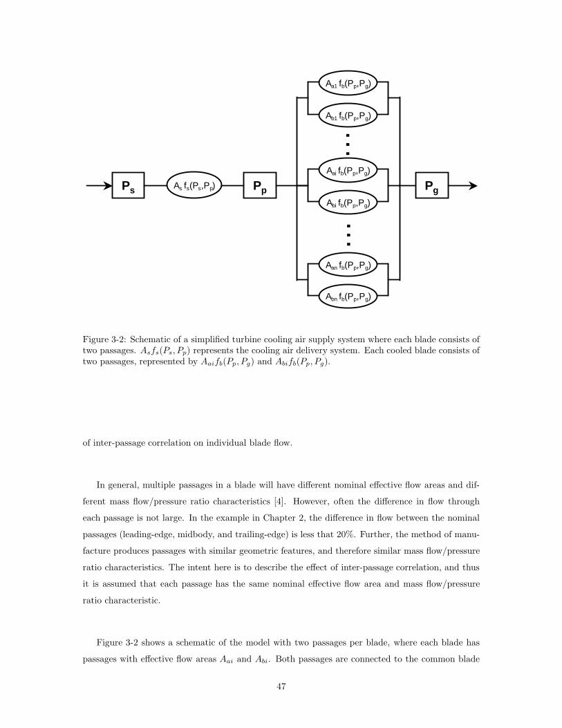
Ps As fs(Ps,Pp) PgPp

…

Aa1 fb(Pp,Pg)

Ab1 fb(Pp,Pg)

Aai fb(Pp,Pg)

Abi fb(Pp,Pg)

Aan fb(Pp,Pg)

Abn fb(Pp,Pg)

…

Figure 3-2: Schematic of a simplified turbine cooling air supply system where each blade consists oftwo passages. Asfs(Ps, Pp) represents the cooling air delivery system. Each cooled blade consists oftwo passages, represented by Aaifb(Pp, Pg) and Abifb(Pp, Pg).

of inter-passage correlation on individual blade flow.

In general, multiple passages in a blade will have different nominal effective flow areas and dif-

ferent mass flow/pressure ratio characteristics [4]. However, often the difference in flow through

each passage is not large. In the example in Chapter 2, the difference in flow between the nominal

passages (leading-edge, midbody, and trailing-edge) is less that 20%. Further, the method of manu-

facture produces passages with similar geometric features, and therefore similar mass flow/pressure

ratio characteristics. The intent here is to describe the effect of inter-passage correlation, and thus

it is assumed that each passage has the same nominal effective flow area and mass flow/pressure

ratio characteristic.

Figure 3-2 shows a schematic of the model with two passages per blade, where each blade has

passages with effective flow areas Aai and Abi. Both passages are connected to the common blade

47

supply plenum Pp. The governing equations of this system can be written as:

m = Asfs(Ps, Pp)

mai = Aaifb(Pp, Pg) i = 1, 2, ..., n

mbi = Abifb(Pp, Pg) i = 1, 2, ..., n

m =

n∑

i=1

(mai + mbi) .

For simplicity, both passages in each blade are assumed to be nominally identical. That is, each

exhibits the same mass flow/pressure ratio characteristic behavior, fb(Pp, Pg), and has the same

nominal effective flow area, Anom. As before for the single-passage model, variability is captured in

the effective area term. Solving the linearized governing equations gives the plenum pressure and

the total system mass flow as:

Pp

(

Anom∂fb

∂Pp

mnom

)

= −1

1 + β

(

1

2n

n∑

i=1

Aai + Abi

Anom

)

(3.4)

˜m

2nmnom=

β

1 + β

(

1

2n

n∑

i=1

Aai + Abi

Anom

)

(3.5)

where β is defined with 2n instead of n:

β ≡ −As

∂fs

∂Pp

2nAnom∂fb

∂Pp

.

Equation (3.4) shows that the plenum pressure is still controlled by the row-average effective area,

where the average is taken over both passages. If both Aai and Abi are low-flowing, with negative

effective area perturbations, Pp will tend to increase.

The flow perturbations in individual blade passages (blade j, passages a and b, for example) are

given by,

˜maj

mnom=

Aaj

Anom−

1

1 + β

(

1

2n

n∑

i=1

Aai + Abi

Anom

)

(3.6)

˜mbj

mnom=

Abj

Anom−

1

1 + β

(

1

2n

n∑

i=1

Aai + Abi

Anom

)

. (3.7)

Both the above individual passage mass flow equations exhibit similar behavior to the previous

simplified model (Equation (3.3)). Each passage’s mass flow is a function of its individual effective

flow area and the average flow area of the entire blade row. For a randomly-assembled, nominally-

centered blade row, where the row-average effective area is zero, the flow through an individual

passage is only a function of the effective area for that passage.

48

To examine the impact of classification combined with correlation between passages on selec-

tively assembled rows, assume that the distributions of effective flow area for the passages can be

characterized by their individual distributions

E[Aai] = µa

E[Abi] = µb

V ar[Aai] = σ2a

V ar[Abi] = σ2b .

Also, assume the correlation between passages can be characterized using a linear correlation coef-

ficient

COV [Aai, Abi] = ρσaσb.

Consider a class consisting of a portion of the distribution of Aai, denoted A∗

ai, with properties

E[A∗

ai] = µ∗

a (3.8)

V ar[A∗

ai] = σ∗

a2. (3.9)

Given the class with µ∗

a and σ∗

a2, the mean and variance of Abi become

E[A∗

bi] = (µ∗

a − µa)ρσb

σa+ µb (3.10)

V ar[A∗

bi] = σ∗

a2

(

ρσb

σa

)2

+ σ2b (1 − ρ2) (3.11)

where A∗

bi denotes the distribution of Abi due to the correlation between the variables and the

classification based on Aai (see Appendix A for the derivation of Equations (3.10) and (3.11)).

Thus, when blades are classified based on one passage, the distribution of effective flow area of

the adjoining passage may also be affected, depending on the amount of inter-passage correlation.

For uncorrelated passages (ρ = 0), the distribution of A∗

bi is unaffected by the classification of

passage a, with E[A∗

bi] = µb and V ar[A∗

bi] = σ2b . For perfectly correlated passages (assuming

σa = σb for simplicity), the distribution of A∗

bi has the same mean shift and variance as A∗

ai, with

E[A∗

bi] = (µ∗

a − µa) + µb and V ar[A∗

bi] = σ∗

a2.

Using Equations (3.8) and (3.10), the mean plenum pressure perturbation is given by:

E[Pp]

(

Anom∂fb

∂Pp

mnom

)

= −1

1 + β

1

2Anom

(

µ∗

a + µb + (µ∗

a − µa)ρσb

σa

)

.

49

The mean total flow perturbation is:

E[ ˜m]

2nmnom=

β

1 + β

1

2Anom

(

µ∗

a + µb + (µ∗

a − µa)ρσb

σa

)

and the mean individual passage flow perturbations are

E[ ˜maj ]

mnom=

µ∗

a

Anom−

1

1 + β

1

2Anom

(

µ∗

a + µb + (µ∗

a − µa)ρσb

σa

)

E[ ˜mbj ]

mnom=

µb

Anom−

1

1 + β

1

2Anom

(

µ∗

a + µb + (µ∗

a − µa)ρσb

σa

)

+1

2Anom(µ∗

a − µa)ρσb

σa.

In each case, the equations depend on the mean of the passage a class (µ∗

a), the mean of passage

b (µb), and a term to modify the mean of passage b based on the classification and correlation

((µ∗

a − µa)ρσb

σa). The modifying term captures the magnitude and sign of the shift from Aai to A∗

ai

((µ∗

a − µa)), a correlation coefficient (ρ) to assign the appropriate direction to the shift from Abi to

A∗

bi, and a scale factor ( σb

σa) to cast the modification in terms of passage b’s variability.

Figure 3-3 illustrates the effects of inter-passage correlation. The top three rows show histograms

of A∗

ai/Anom, A∗

bi/Anom, and Pp

(

Anom∂fb

∂Pp/mnom

)

for three different values of correlation coeffi-

cient, ρ = −1, ρ = 0, and ρ = 1 (assuming β = 0). The distribution of A∗

ai/Anom has been selected

such that it consists of low-flow passages only. In the case of perfectly correlated areas (ρ = 1, shown

in the right column of Figure 3-3), the distributions of A∗

ai/Anom and A∗

bi/Anom are identical and the

mean value of the plenum pressure, Pp

(

Anom∂fb

∂Pp/mnom

)

, is maximized. When the areas are com-

pletely uncorrelated (ρ = 0, shown in the center column of Figure 3-3), the variability of A∗

bi/Anom

is unchanged and the increase in Pp is reduced. If the passages exhibit perfect negative correlation

(ρ = −1), then the low-flow A∗

ai/Anom ensures high-flow A∗

bi/Anom. This produces a row-average

effective area of zero, eliminating the pressure compensation benefit of selective assembly.

The two bottom rows in Figure 3-3 show distributions of individual passage a flow for all

blades(

˜maj/mnom

)

and individual passage a flow for the lowest-flow passage in each blade row(

minj=1...n

(

˜maj/mnom

))

. The minimum passage a flow tends toward the left tail of the distribu-

tions of all individual passage a flows. The minimum flow passage is also the minimum life blade, so

the distributions of minimum blade flow are equivalent to distributions of engine life due to turbine

blade oxidation. Therefore, to improve engine life, the minimum passage flow must be increased.

3.6 Impact of Selective Assembly on Turbine Inlet Temper-

ature

As described in Sections 3.3 and 3.5, selective assembly segregates the lowest-flow blades and in-

creases the amount of coolant flow delivered to them, leading to lower blade metal temperatures

50

−0.2 0 0.2

ρ = 0

−0.2 0 0.2

−0.1 0 0.1

−0.2 0 0.2

ρ = −1

Aaj

Anom

_____

−0.2 0 0.2

Abj

Anom

_____

−0.1 0 0.1

Pp

Anom ∂ fb

∂ Pp

_____

mnom

_________

−0.2 0 0.2

ρ = 1

−0.2 0 0.2

−0.1 0 0.1

−0.2 0 0.2

maj

mnom

_____

−0.2 0 0.2 −0.2 0 0.2

−0.2 0 0.2

min maj

mnom

_____

−0.2 0 0.2 −0.2 0 0.2

.

.

.

.

.

Figure 3-3: Histograms of passage areas (Aai/Anom and Abi/Anom), blade plenum pressure

(Pp

(

Anom∂fb

∂Pp/mnom

)

), individual blade flow ((

˜maj/mnom

)

), and the lowest blade flow in each

blade row ((

minj=1...n

(

˜maj/mnom

))

) for three levels of area correlation from the two passage sim-

plified model (assuming β = 0). The distribution of Aai/Anom has been selected such that it consistsof low-flow passages only.

and longer life. Alternatively, selective assembly can be used to allow blades to withstand increased

turbine inlet temperature while maintaining the maximum blade material temperatures at current

(random-assembly) levels.

This section addresses the benefits in turbine inlet temperature for selective assembly. To achieve

these results, the rest of the turbine hardware (vanes and outer airseals) will also experience increased

temperature. If these components do not have sufficient life at the elevated temperatures, they would

require redesign. However, since the first-stage blades dictate the useable interval for the example

engine model considered, it is likely that the remaining components have some amount of additional

life capability available.

In Chapter 4, the impact of selective assembly on the probabilistic analysis shown in Chapter 2

will be presented. Here, using the two-passage simplified flow model, the implications of selective

assembly on turbine inlet temperature can be estimated in a generic manner. Specifically, given

51

the distributions of blade effective area for the two passages, Aai and Abi, with the appropriate

correlation, ρ, rows of turbine blades can be assembled and the mass flow through each blade in a

row can be estimated using Equations (3.6) and (3.7). This analysis will assume that the effective

flow area of each passage is normally distributed with a coefficient of variation of 5% (which is

representative of actual bench flow data from production).

Given the mass flow in a blade passage, the metal temperature can be estimated using the

procedure employed in Chapter 2. The cooling effectiveness is defined as

η ≡Tgas − Tmetal

Tmetal − Tcool

and is assumed to behave as,

η = ηb

(

mj

mb

)0.8

,

where ηb is the nominal value of η attained when the mass flow is the nominal value, mj = mnom.

ηb is determined from the design intent blade cooling effectiveness, where the cooling effectiveness

is defined as,

φ ≡Tgas − Tmetal

Tgas − Tcool.

From the definitions of η and φ, η = φ/(1 − φ) and therefore, ηb = φb/(1 − φb). The examples are

based on Tgas − Tcool = 1825◦F .

The blade flow classes are shown in Figure 3-4, determined using passage a. The figure shows a

distribution of measured flows for a blade passage, divided into three classes: low-flow, nominal-flow,

and high-flow. Blade rows randomly assembled from the entire distribution of blade flows will be

referred to as Random Assembly sets.

Figure 3-5 shows the relationship between allowable turbine inlet temperature increase and β

for three values of nominal cooling effectiveness for the low-flow fleet, with an inter-passage cor-

relation ρ = 0. To generate these values, turbine inlet temperature is varied until the worst-case

(95thpercentile) blade metal temperatures are the same for a Random Assembly fleet and a low-flow

fleet. Smaller values of β and higher values of φb permit larger increases in turbine inlet temperature.

For example, for φb = 0.5 and β = 1.5, applying the selective assembly method enables an increase

in turbine inlet temperature by about 7◦F . If β = 0, the turbine inlet temperature increase is about

25◦F .

Figure 3-6 shows the relationship between turbine inlet temperature increase and β for three

different blade passage flow classes, given a nominal cooling effectiveness φb = 0.5 and no inter-

passage correlation ρ = 0. The low-flow class allows larger increases in turbine inlet temperature

as β decreases. The turbine inlet temperature increase for the nominal-flow fleet is insensitive to

changes in β, while the curve for the high-flow fleet shows that larger values of β allow for larger

52

Leading Edge Flow Capability

Low−Flow Nominal−Flow High−Flow

−3σ −1σ +1σ +3σ

Figure 3-4: The distribution of manufactured flow capability is divided into three flow classes fordemonstration of selective assembly of turbine blade rows.

increases in turbine inlet temperature. These trends can also be explained by consideration of how

the individual blade flows behave for these classes using Equation (3.6). For the nominal flow class,

the row-average effective area perturbation would be zero (in the mean); thus, the value of β will

not enter and the plenum pressure will be the nominal value. For a high-flow class, the row-effective

area is positive, thus β affects the individual blade flows. As in the low-flow case, low values of β

will cause the total flow to approach the nominal total flow. For the high-flow case, however, this

would lower the individual flow through these high-flow blades since for higher β these blades would

draw more air from the supply system.

Figure 3-7 shows the relationship between turbine inlet temperature increase and β for three

levels of inter-passage correlation, assuming low-flow classes and a nominal cooling effectiveness

φb = 0.5. Both the perfectly correlated, ρ = 1, and the uncorrelated, ρ = 0, cases show larger

turbine inlet temperature increases as β decreases. The perfectly correlated case allows for a greater

turbine inlet temperature increase because perfect correlation between the passages maximizes the

blade plenum pressure compensation and minimizes the flow variability in the passages. The case

with perfect negative correlation produces lower passage a flows than the Random Assembly case,

so the turbine inlet temperature must be decreased to match the worst-case metal temperature from

the Random Assembly case.

The allowable turbine inlet temperature increase results can be used to compare the relative

effect of each parameter. Consider a nominal-flow class where β = 0, φ = 0.5, and ρ = 0. The effect

53

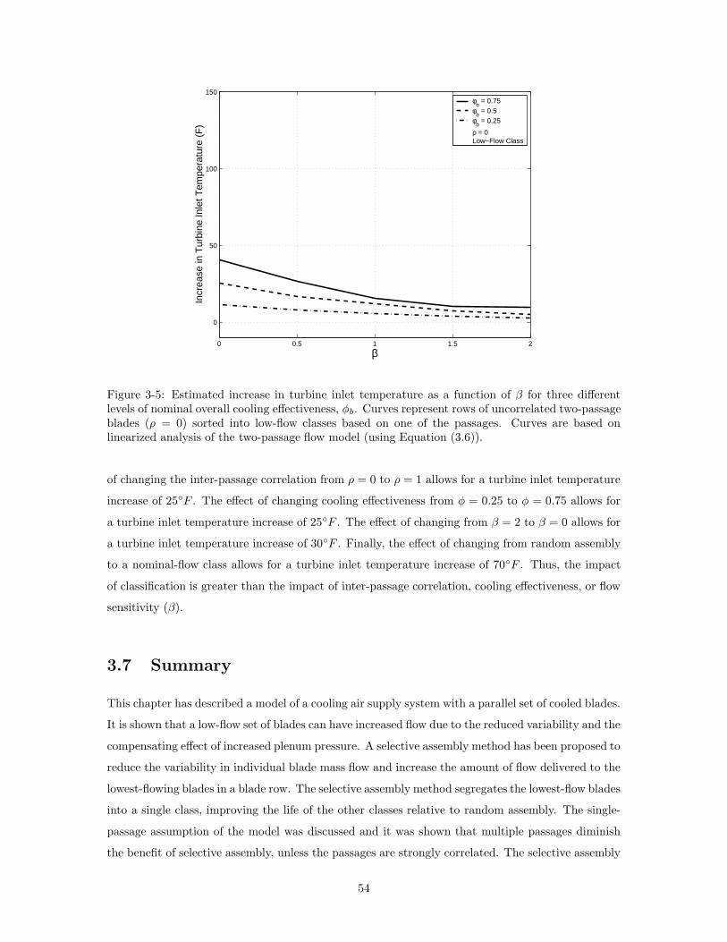
0 0.5 1 1.5 2

0

50

100

150

β

Incr

ease

in T

urbi

ne In

let T

empe

ratu

re (

F)

φb = 0.75

φb = 0.5

φb = 0.25

ρ = 0 Low−Flow Class

Figure 3-5: Estimated increase in turbine inlet temperature as a function of β for three differentlevels of nominal overall cooling effectiveness, φb. Curves represent rows of uncorrelated two-passageblades (ρ = 0) sorted into low-flow classes based on one of the passages. Curves are based onlinearized analysis of the two-passage flow model (using Equation (3.6)).

of changing the inter-passage correlation from ρ = 0 to ρ = 1 allows for a turbine inlet temperature

increase of 25◦F . The effect of changing cooling effectiveness from φ = 0.25 to φ = 0.75 allows for

a turbine inlet temperature increase of 25◦F . The effect of changing from β = 2 to β = 0 allows for

a turbine inlet temperature increase of 30◦F . Finally, the effect of changing from random assembly

to a nominal-flow class allows for a turbine inlet temperature increase of 70◦F . Thus, the impact

of classification is greater than the impact of inter-passage correlation, cooling effectiveness, or flow

sensitivity (β).

3.7 Summary

This chapter has described a model of a cooling air supply system with a parallel set of cooled blades.

It is shown that a low-flow set of blades can have increased flow due to the reduced variability and the

compensating effect of increased plenum pressure. A selective assembly method has been proposed to

reduce the variability in individual blade mass flow and increase the amount of flow delivered to the

lowest-flowing blades in a blade row. The selective assembly method segregates the lowest-flow blades

into a single class, improving the life of the other classes relative to random assembly. The single-

passage assumption of the model was discussed and it was shown that multiple passages diminish

the benefit of selective assembly, unless the passages are strongly correlated. The selective assembly

54

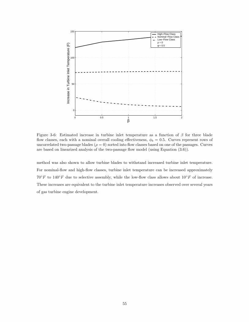
0 0.5 1 1.5 2

0

50

100

150

β

Incr

ease

in T

urbi

ne In

let T

empe

ratu

re (

F)

High−Flow Class Nominal−Flow ClassLow−Flow Class ρ = 0 φ = 0.5

Figure 3-6: Estimated increase in turbine inlet temperature as a function of β for three bladeflow classes, each with a nominal overall cooling effectiveness, φb = 0.5. Curves represent rows ofuncorrelated two-passage blades (ρ = 0) sorted into flow classes based on one of the passages. Curvesare based on linearized analysis of the two-passage flow model (using Equation (3.6)).

method was also shown to allow turbine blades to withstand increased turbine inlet temperature.

For nominal-flow and high-flow classes, turbine inlet temperature can be increased approximately

70◦F to 140◦F due to selective assembly, while the low-flow class allows about 10◦F of increase.

These increases are equivalent to the turbine inlet temperature increases observed over several years

of gas turbine engine development.

55

0 0.5 1 1.5 2

0

50

100

150

β

Incr

ease

in T

urbi

ne In

let T

empe

ratu

re (

F)

ρ = 1 ρ = 0 ρ = −1 φ = 0.5 Low−Flow Class

Figure 3-7: Estimated increase in turbine inlet temperature as a function of β for three levels of inter-passage correlation, each with a nominal overall cooling effectiveness, φb = 0.5. Curves representrows of two-passage blades sorted into low-flow classes based on one of the passages. Curves arebased on linearized analysis of the two-passage flow model (using Equation (3.6)).

56

Chapter 4

Application of Selective Assembly

to a Commercial Turbofan

4.1 Introduction

This chapter considers the application of the selective assembly method to the first turbine rotor

of the commercial turbofan described in Chapter 2. Probabilistic simulations of the auxiliary air

system of this turbofan are used to quantify the benefits of the selective assembly process on blade

flow, metal temperature, and engine life due to oxidation damage for a representative population of

blades.

As related in Section 2.2, the entire auxiliary air system is described using a network flow model

in which all the blades in the row of interest are included as separate elements. The blade metal

temperature and oxidation life are calculated at a variety of points on the airfoil surface using a

flow-scaling analysis.

The first turbine rotor blades for this turbofan consist of three cooling passages: a leading-edge

passage, a midbody passage, and a trailing edge passage. The flow capability of each passage is

measured after manufacture to ensure it is within acceptable limits. These data also provide the

correlation in flow between each passage. The model includes this inter-passage correlation in the

probabilistic simulations of the auxiliary air system. In this example, the passages have a weak

positive correlation, with correlation coefficients less than 0.25.

In addition to individual blade flow variability, the probabilistic simulations include other relevant

sources of variability within the engine. These include engine-to-engine variability in gas path

conditions (temperatures, pressures, rotational speeds), geometric variability within the cooling air

delivery system (hole diameters, radii from engine centerline, rotating seal clearances, effective areas

of flow components), and engine deterioration effects. Description of the included variabilities is

57

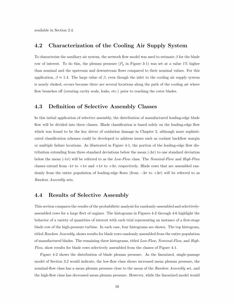
available in Section 2.4.

4.2 Characterization of the Cooling Air Supply System

To characterize the auxiliary air system, the network flow model was used to estimate β for the blade

row of interest. To do this, the plenum pressure (Pp in Figure 3-1) was set at a value 1% higher

than nominal and the upstream and downstream flows compared to their nominal values. For this

application, β ≈ 1.4. The large value of β, even though the inlet to the cooling air supply system

is nearly choked, occurs because there are several locations along the path of the cooling air where

flow branches off (rotating cavity seals, leaks, etc.) prior to reaching the rotor blades.

4.3 Definition of Selective Assembly Classes

In this initial application of selective assembly, the distribution of manufactured leading-edge blade

flow will be divided into three classes. Blade classification is based solely on the leading-edge flow

which was found to be the key driver of oxidation damage in Chapter 2, although more sophisti-

cated classification schemes could be developed to address issues such as coolant backflow margin

or multiple failure locations. As illustrated in Figure 4-1, the portion of the leading-edge flow dis-

tribution extending from three standard deviations below the mean (-3σ) to one standard deviation

below the mean (-1σ) will be referred to as the Low-Flow class. The Nominal-Flow and High-Flow

classes extend from -1σ to +1σ and +1σ to +3σ, respectively. Blade rows that are assembled ran-

domly from the entire population of leading-edge flows (from −3σ to +3σ) will be referred to as

Random Assembly sets.

4.4 Results of Selective Assembly

This section compares the results of the probabilistic analysis for randomly-assembled and selectively-

assembled rows for a large fleet of engines. The histograms in Figures 4-2 through 4-6 highlight the

behavior of a variety of quantities of interest with each trial representing an instance of a first-stage

blade row of the high-pressure turbine. In each case, four histograms are shown. The top histogram,

titled Random Assembly, shows results for blade rows randomly assembled from the entire population

of manufactured blades. The remaining three histograms, titled Low-Flow, Nominal-Flow, and High-

Flow, show results for blade rows selectively assembled from the classes of Figure 4-1.

Figure 4-2 shows the distribution of blade plenum pressure. As the linearized, single-passage

model of Section 3.2 would indicate, the low-flow class shows increased mean plenum pressure, the

nominal-flow class has a mean plenum pressure close to the mean of the Random Assembly set, and

the high-flow class has decreased mean plenum pressure. However, while the linearized model would

58

Leading Edge Flow Capability

Low−Flow Nominal−Flow High−Flow

−3σ −1σ +1σ +3σ

Figure 4-1: The distribution of manufactured flow capability is divided into three flow classes (Low-

Flow, Nominal-Flow, and High-Flow) for demonstration of selective assembly of turbine blade rows.

indicate a decrease in plenum pressure variability due to classification, the variability of plenum

pressure is similar for Random Assembly and the selective assembly classes. The reason is that the

effective area variabilities of the midbody and trailing edge passages are relatively unaffected by

the leading-edge classification scheme due to the weak correlations among the different passages.

Section 3.5 demonstrated the effect of multiple, uncorrelated passages on the variability of blade

plenum pressure on a selectively assembled class of blades.

Figure 4-3 shows the distribution of blade leading-edge passage flow. The trends are consistent

with the linearized, single-passage model. The low-flow class, which has a decreased mean effective

area, shows a decrease in leading-edge flow. Similarly, the high-flow class, which has an increased

mean effective area, shows an increase in leading-edge flow. The selectively assembled classes show

decreases in the variability of the leading-edge flow relative to the Random Assembly rows since the

classification directly reduces the variability of the leading-edge flow effective area.

As discussed above, the lowest life blade in the row is expected to be the blade with the lowest

flow. In this case, since the dominant failure mechanism occurs at the leading edge, the lowest

leading-edge flow in the row is the critical life-limiting quantity. Figure 4-4 shows the distribution of

the lowest-flowing leading edge in each row, plotted on the same scale as Figure 4-3. These lowest-

flow blades come from the left tails of the distributions shown in Figure 4-3. As a result, the low-flow

class in Figure 4-4 has a distribution which is similar to the Random Assembly set. The nominal-flow

sets have about 5% higher minimum flow than either the low-flow class or Random Assembly rows,

59

0.99 1 1.01

Random Assembly µ = 1.000, σ = 0.003

0.99 1 1.01

Low−Flow µ = 1.003, σ = 0.003

0.99 1 1.01

Nominal−Flow µ = 1.000, σ = 0.003

0.99 1 1.01

Blade Plenum Pressure

High−Flow µ = 0.997, σ = 0.003

Figure 4-2: Histograms showing blade plenum pressure for randomly assembled and selectively as-sembled blade rows. Plenum pressures have been non-dimensionalized by the mean plenum pressurefor the randomly-assembled rows.

and high-flow sets are another 5% higher.

Figure 4-5 shows the distribution of the maximum blade metal temperature in a row. These

results are similar to the worst-flow results of Figure 4-4. Specifically, the low-flow class maximum

blade temperatures have a slightly higher mean but smaller variability than the Random Assembly

set and the nominal-flow and high-flow classes show lower maximum metal temperatures with an

approximately 0.75% drop for each class.

Figure 4-6 shows the impact of selective assembly on turbine life due to high-temperature oxi-

dation. The behavior corresponds to that of the minimum leading-edge flow and maximum metal

temperature. The low-flow class rows have a slightly lower mean life (3%) than the Random As-

sembly set but with less variability. The nominal-flow class has a mean life that is 38% higher

than the Random Assembly set and the high-flow class has a mean life that is 84% higher than the

Random Assembly set. For gas turbine operators, estimates of the B5 life (5 out of 100 cumulative

probability) are frequently used to set the required maintenance intervals in an effort to reduce the

frequency of unscheduled repairs. Post-processing the distributions depicted in Figure 4-6 shows

that the B5 life of the low-flow, nominal-flow, and high-flow rows are 3%, 52%, and 106% higher

than the Random Assembly set, respectively (worst-case at 95% confidence: -0.8%, 48%, and 101%).

To place into perspective the impact of selective assembly on turbine oxidation life, the relative

manufacturing frequency of each class should be considered. For example, measured flow data shows

60

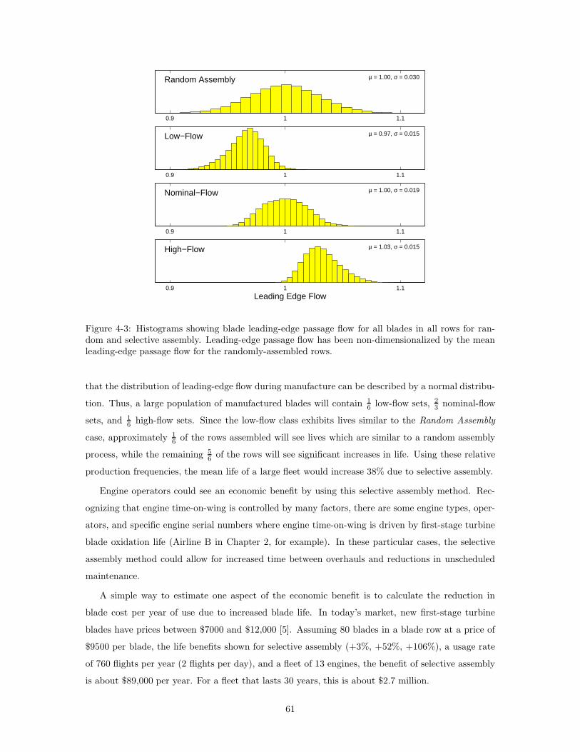
0.9 1 1.1

µ = 1.00, σ = 0.030Random Assembly

0.9 1 1.1

µ = 0.97, σ = 0.015Low−Flow

0.9 1 1.1

µ = 1.00, σ = 0.019Nominal−Flow

0.9 1 1.1

Leading Edge Flow

µ = 1.03, σ = 0.015High−Flow

Figure 4-3: Histograms showing blade leading-edge passage flow for all blades in all rows for ran-dom and selective assembly. Leading-edge passage flow has been non-dimensionalized by the meanleading-edge passage flow for the randomly-assembled rows.

that the distribution of leading-edge flow during manufacture can be described by a normal distribu-

tion. Thus, a large population of manufactured blades will contain 16 low-flow sets, 2

3 nominal-flow

sets, and 16 high-flow sets. Since the low-flow class exhibits lives similar to the Random Assembly

case, approximately 16 of the rows assembled will see lives which are similar to a random assembly

process, while the remaining 56 of the rows will see significant increases in life. Using these relative

production frequencies, the mean life of a large fleet would increase 38% due to selective assembly.

Engine operators could see an economic benefit by using this selective assembly method. Rec-

ognizing that engine time-on-wing is controlled by many factors, there are some engine types, oper-

ators, and specific engine serial numbers where engine time-on-wing is driven by first-stage turbine

blade oxidation life (Airline B in Chapter 2, for example). In these particular cases, the selective

assembly method could allow for increased time between overhauls and reductions in unscheduled

maintenance.

A simple way to estimate one aspect of the economic benefit is to calculate the reduction in

blade cost per year of use due to increased blade life. In today’s market, new first-stage turbine

blades have prices between $7000 and $12,000 [5]. Assuming 80 blades in a blade row at a price of

$9500 per blade, the life benefits shown for selective assembly (+3%, +52%, +106%), a usage rate

of 760 flights per year (2 flights per day), and a fleet of 13 engines, the benefit of selective assembly

is about $89,000 per year. For a fleet that lasts 30 years, this is about $2.7 million.

61

0.9 0.95 1 1.05


0.9 0.95 1 1.05

µ = 0.93, σ = 0.011Low−Flow

0.9 0.95 1 1.05


0.9 0.95 1 1.05

Minimum Leading Edge Flow

µ = 1.02, σ = 0.010High−Flow

Figure 4-4: Histograms showing minimum blade leading-edge passage flow in each blade row forrandom and selective assembly, plotted on the same scale as Figure 4-3.

While improved blade life is possible by increasing the total amount of coolant flow delivered

to the blades, an increase in coolant flow has a detrimental effect on the efficiency of the engine.

However, as described in the discussion of the linearized, single-passage model, the improvements

in blade life when using the proposed selective assembly are not due to increases in the total flow

for the entire population of rows but rather are tied to the reduction blade-to-blade flow variability

within a row. To demonstrate this, the low-flow, nominal-flow, and high-flow classes are combined

with their relative production frequencies (i.e. 16 , 2

3 , and 16 respectively), and the distribution of

total flow is compared for the selective and random assembly populations. As shown in Figure 4-7,

the distributions of total flow are nearly identical, indicating that the amount of total coolant flow

for a large fleet of engines is unchanged due to selective assembly.

A simple cycle analysis of a turbofan can quantify the effect on engine performance due to changes

in the amount of turbine cooling flow. Engine performance parameters are available in the literature

62

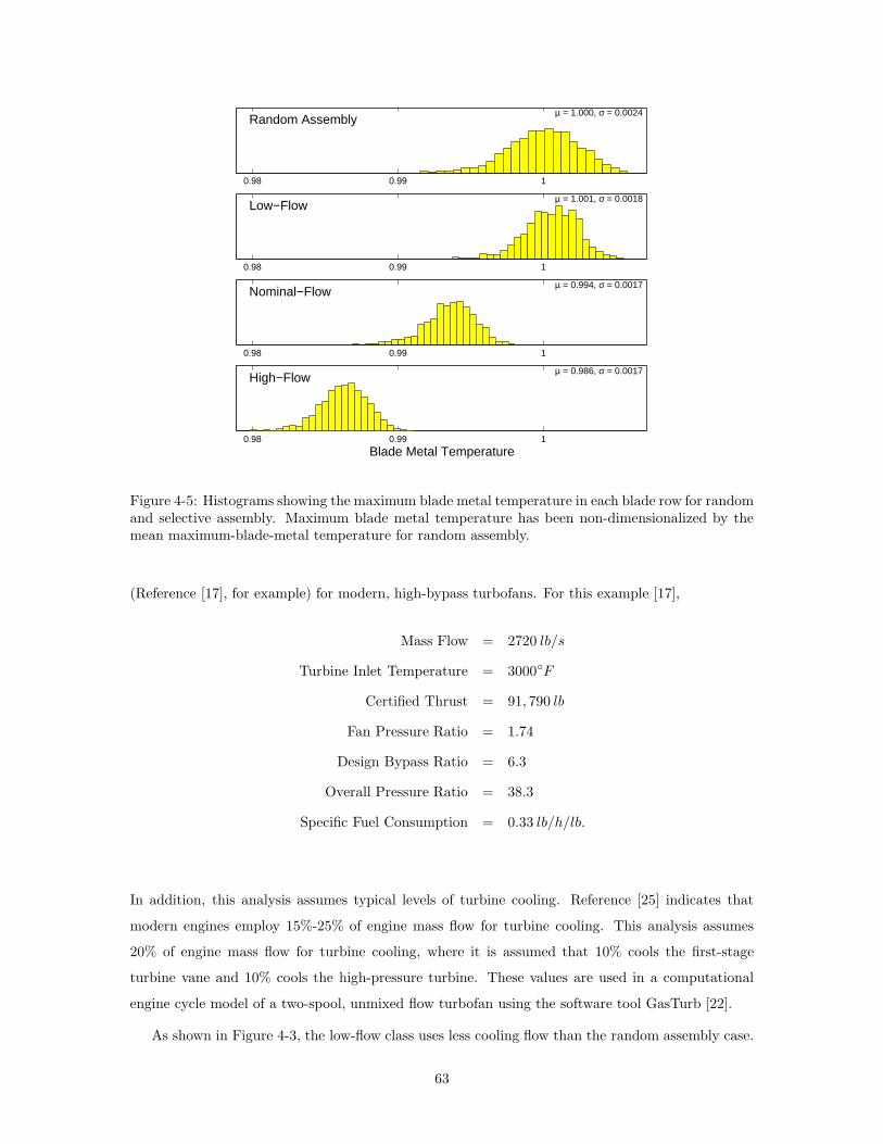
0.98 0.99 1


0.98 0.99 1

µ = 1.001, σ = 0.0018Low−Flow

0.98 0.99 1

µ = 0.994, σ = 0.0017Nominal−Flow

0.98 0.99 1

Blade Metal Temperature

µ = 0.986, σ = 0.0017High−Flow

Figure 4-5: Histograms showing the maximum blade metal temperature in each blade row for randomand selective assembly. Maximum blade metal temperature has been non-dimensionalized by themean maximum-blade-metal temperature for random assembly.

(Reference [17], for example) for modern, high-bypass turbofans. For this example [17],

Mass Flow = 2720 lb/s

Turbine Inlet Temperature = 3000◦F

Certified Thrust = 91, 790 lb

Fan Pressure Ratio = 1.74

Design Bypass Ratio = 6.3

Overall Pressure Ratio = 38.3

Specific Fuel Consumption = 0.33 lb/h/lb.

In addition, this analysis assumes typical levels of turbine cooling. Reference [25] indicates that

modern engines employ 15%-25% of engine mass flow for turbine cooling. This analysis assumes

20% of engine mass flow for turbine cooling, where it is assumed that 10% cools the first-stage

turbine vane and 10% cools the high-pressure turbine. These values are used in a computational

engine cycle model of a two-spool, unmixed flow turbofan using the software tool GasTurb [22].

As shown in Figure 4-3, the low-flow class uses less cooling flow than the random assembly case.

63

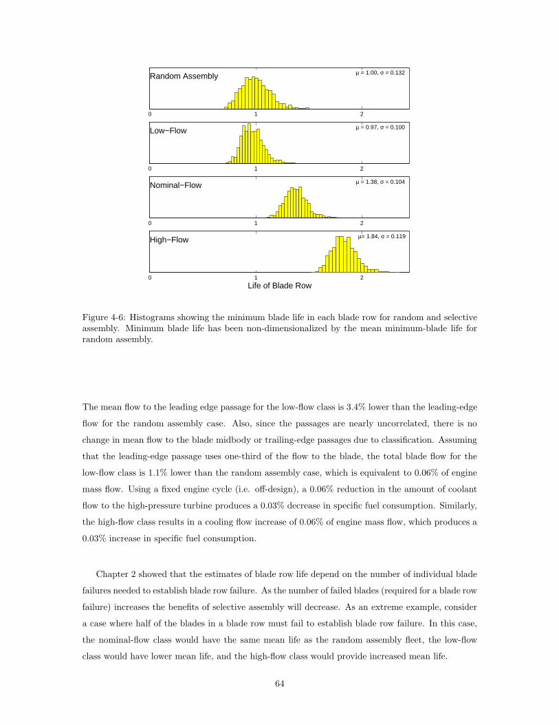
0 1 2


0 1 2

µ = 0.97, σ = 0.100Low−Flow

0 1 2


0 1 2

Life of Blade Row

µ= 1.84, σ = 0.119High−Flow

Figure 4-6: Histograms showing the minimum blade life in each blade row for random and selectiveassembly. Minimum blade life has been non-dimensionalized by the mean minimum-blade life forrandom assembly.

The mean flow to the leading edge passage for the low-flow class is 3.4% lower than the leading-edge

flow for the random assembly case. Also, since the passages are nearly uncorrelated, there is no

change in mean flow to the blade midbody or trailing-edge passages due to classification. Assuming

that the leading-edge passage uses one-third of the flow to the blade, the total blade flow for the

low-flow class is 1.1% lower than the random assembly case, which is equivalent to 0.06% of engine

mass flow. Using a fixed engine cycle (i.e. off-design), a 0.06% reduction in the amount of coolant

flow to the high-pressure turbine produces a 0.03% decrease in specific fuel consumption. Similarly,

the high-flow class results in a cooling flow increase of 0.06% of engine mass flow, which produces a

0.03% increase in specific fuel consumption.

Chapter 2 showed that the estimates of blade row life depend on the number of individual blade

failures needed to establish blade row failure. As the number of failed blades (required for a blade row

failure) increases the benefits of selective assembly will decrease. As an extreme example, consider

a case where half of the blades in a blade row must fail to establish blade row failure. In this case,

the nominal-flow class would have the same mean life as the random assembly fleet, the low-flow

class would have lower mean life, and the high-flow class would provide increased mean life.

64

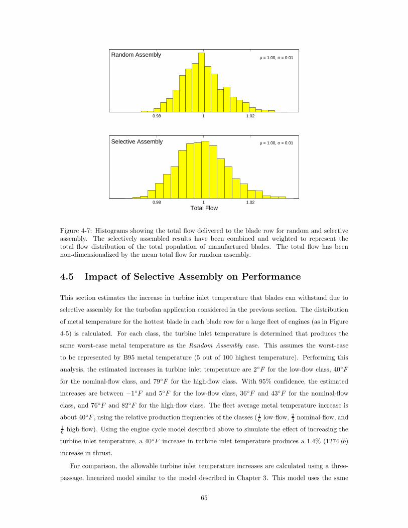
0.98 1 1.02


0.98 1 1.02

Total Flow

µ = 1.00, σ = 0.01Selective Assembly

Figure 4-7: Histograms showing the total flow delivered to the blade row for random and selectiveassembly. The selectively assembled results have been combined and weighted to represent thetotal flow distribution of the total population of manufactured blades. The total flow has beennon-dimensionalized by the mean total flow for random assembly.

4.5 Impact of Selective Assembly on Performance

This section estimates the increase in turbine inlet temperature that blades can withstand due to

selective assembly for the turbofan application considered in the previous section. The distribution

of metal temperature for the hottest blade in each blade row for a large fleet of engines (as in Figure

4-5) is calculated. For each class, the turbine inlet temperature is determined that produces the

same worst-case metal temperature as the Random Assembly case. This assumes the worst-case

to be represented by B95 metal temperature (5 out of 100 highest temperature). Performing this

analysis, the estimated increases in turbine inlet temperature are 2◦F for the low-flow class, 40◦F

for the nominal-flow class, and 79◦F for the high-flow class. With 95% confidence, the estimated

increases are between −1◦F and 5◦F for the low-flow class, 36◦F and 43◦F for the nominal-flow

class, and 76◦F and 82◦F for the high-flow class. The fleet average metal temperature increase is

about 40◦F , using the relative production frequencies of the classes ( 16 low-flow, 2

3 nominal-flow, and

16 high-flow). Using the engine cycle model described above to simulate the effect of increasing the

turbine inlet temperature, a 40◦F increase in turbine inlet temperature produces a 1.4% (1274 lb)

increase in thrust.

For comparison, the allowable turbine inlet temperature increases are calculated using a three-

passage, linearized model similar to the model described in Chapter 3. This model uses the same

65

blade passage variability and inter-passage correlations as the probabilistic analysis described above.

This allows turbine inlet temperature increases of 4◦F for the low-flow class, 44◦F for the nominal-

flow class, and 83◦F for the high-flow class. These linearized model results are similar to the

allowable turbine inlet temperature increases from the above probabilistic analysis, indicating that

the three-passage, linearized model provides a good estimate of the behavior of the full probabilistic

analysis.

Note that engine manufacturers permit different turbine temperature limits depending on the

specific operator’s requirements. In the current row assembly process which does not consider

blade flow capability (beyond some limits of acceptability), any negotiated increases in allowable

turbine temperature would result in decreased life, more frequent inspections, or both. However,

using selective assembly, an engine manufacturer could allow higher temperature operation while

decreasing the impact on life by prescribing the use of blades from nominal-flow or high-flow classes.

Also, these high-performance blade sets could be sold at a premium price. Thus, in practice, the

potential of selectively-assembled rows to operate at different maximum turbine inlet temperatures

could be utilized.

First, as given in Section 3.6, the recent rate of increase in turbine inlet temperature is about

6◦F per year. Therefore, the increases in turbine inlet temperature estimated using the full turbofan

model are quite significant, equivalent to several years of gas turbine engine development. Second,

though this thesis has not investigated this possibility, the potential exists that the impact of selective

assembly could be improved by a more sophisticated classification scheme in which all passages in a

blade are considered.

Engine sales prices tend to correlate with sea-level takeoff thrust. Large engines tend to have

prices around $140 per pound of thrust [17]. Therefore, the estimated increase in thrust would allow

the engine manufacturer to increase engine price by $178,000 per engine. For a fleet of 82 engines

(like Airline A), this increases revenue by $14.6 million.

4.6 Summary

To demonstrate the potential of the selective assembly process, this chapter presented a probabilistic

analysis of an existing high-bypass turbofan focusing on the oxidation life of the first turbine rotor. A

simple classification scheme was utilized in which the blades were classed into low-flow, nominal-flow,

and high-flow sets. For these respective classes, the analysis of the first turbine rotor estimates that

the B5 life would be 3%, 52%, and 106% higher than a random assembly process. Alternatively,

selective assembly can be used to allow blades to withstand increased turbine inlet temperature

while maintaining the maximum blade metal temperatures at current (random assembly) levels. An

analysis of the potential for increased turbine inlet temperature showed that a linearized, three-

66

passage model can closely match the behavior of a higher-fidelity analysis. For the nominal-flow and

high-flow classes in the turbofan application, turbine inlet temperature increases are estimated to

be equivalent to several years of gas turbine technology development.

67

Chapter 5

Summary and Recommendations

5.1 Summary

Chapter 2 presented a probabilistic methodology to determine the effect of component variability

on the cooling flow and oxidation life of a row of turbine blades. The method used a Monte Carlo

approach to propagate known variability in input parameters through an analysis to characterize

the distribution of turbine oxidation life.

This chapter showed that it is critical that the network flow model individually represent every

blade in a blade row to accurately estimate individual blade flow and therefore blade-row oxidation

life. Including every blade individually increases the probability of observing a low-flow (low-life)

blade within a blade row. Further, all blades must be allowed to individually vary to capture

the correct behavior of the cooling air delivery system, and thus accurately estimate blade metal

temperature and life.

A distribution of the probability of oxidation failure was generated for each of two airlines. The

probabilistic distributions of failure times were compared to the field failure distributions of two

airlines and were shown to better capture the difference between a typical engine fleet and a fleet

operating in a hotter environment as compared to current practice.

Using regression analysis, the results of Monte Carlo analysis were used to establish the relative

effect of each input parameter’s variability on the distribution of turbine oxidation life, specifically

identifying which input variabilities drive turbine life. For both airlines, a 10% decrease in the

variability of blade leading edge effective flow area can have an impact on both the typical and

minimum life. For Airline B, this variability decrease can increase the minimum oxidation life of the

engine model by 33%.

Chapter 3 described a simplified model of a cooling air supply system with a parallel set of

cooled blades. This chapter demonstrated that the flow through an individual blade is a function

69

of both its individual flow area and the average-flow area of all blades assembled in the row. In

particular, the blade plenum pressure tends to increase with decreased average-blade flow area. As

a result, the individual blade flow for a row assembled entirely from low-flow blades will tend to be

closer to the design intent than for a single low-flow blade in a randomly-assembled row. Based on

this, a method of selectively assembling rows of turbine blades by flow class was proposed that can

reduce the variability in individual blade mass flow and increase the amount of flow delivered to

the lowest-flowing blades in a blade row. In addition, the selective assembly method segregates the

lowest-flow blades into a single class, significantly improving the performance of the other classes.

The single-passage assumption of the simplified model was discussed and it was shown that multiple

passages can diminish the benefit of selective assembly, unless the passages are strongly correlated.

In addition, Chapter 3 has shown that the selective assembly method can be used to allow blades to

withstand an increase in turbine inlet temperature. For nominal-flow and high-flow classes, turbine

inlet temperature can be increased approximately 70◦F to 140◦F due to selective assembly, while

the low-flow class still allows about 10◦F of increase.

To demonstrate the potential of the selective assembly process, Chapter 4 described a proba-

bilistic analysis of an existing high-bypass turbofan focusing on the oxidation life of the first turbine

rotor. A simplified classification scheme was utilized in which the blades were classed into low-flow,

nominal-flow, and high-flow sets. For these respective classes, the analysis of the first turbine rotor

estimated that the B5 life would be 3%, 52%, and 106% higher than a random assembly process.

Alternatively, selective assembly can be used to increase turbine inlet temperature while maintaining

the maximum blade metal temperatures at current (random assembly) levels. For the nominal-flow

and high-flow classes, turbine inlet temperature increases are estimated to be equivalent to the tur-

bine inlet temperature increases observed over several years of gas turbine technology development.

5.2 Recommendations for Future Work

This thesis has shown the importance of using a probabilistic approach and of individually rep-

resenting every blade in a blade row for network flow models of an engine’s auxiliary air system.

Therefore, in order to improve the estimates of flow through turbine blade cooling passages (and

subsequently, life), it is recommended to probabilistically analyze auxiliary air system models and

to individually represent every blade within these models.

This research can be extended in three broad categories: (1) improvement of the analytical

models, (2) development of more sophisticated classification schemes, and (3) addressing of logistical

problems associated with the application of the selective assembly method.

The models used in this thesis have been adequate to identify the dominant mechanisms and the

controlling parameters, but they are all somewhat simplified. If better predictions of coolant flow

70

and blade life are required, the models should be improved. This analysis modeled each flow passage

in the blade using a single mass flow / pressure ratio relationship. It would be more accurate to

extend the network flow model to capture all the flow features within the blade. In addition, the

calculation of blade metal temperature should be improved, including the ability to capture local

changes in internal and external heat transfer coefficients and cooling effectiveness. Also, there are

other physical phenomena that are difficult to analytically capture, the effects of sand ingestion, for

example, that could impact the life of turbine blades.

This thesis focused on the oxidation life of a single, life-limiting location on blades in a particular

row within the high-pressure turbine. Although many blade designs have a single life-limiting loca-

tion, others have several locations that can limit the blade’s life. The scope of the analysis could be

extended to account for multiple oxidation failure locations on each blade, ultimately assessing the

life of the entire blade by accounting for the variation in failure location. Other failure modes could

also be included, creep and thermo-mechanical fatigue, for example. Furthermore, multiple blade

(and vane) rows could be included in the analysis in order to allow a variety of locations within the

turbine to limit an engine model’s life.

An example application of selective assembly of turbine blades was described in Chapter 4 that

used a simple three-class selection scheme. While the benefits of selective assembly were significant

using this classification scheme, the potential exists to improve upon the results by developing more

sophisticated classification schemes. An optimized classification scheme could balance blade pro-

duction frequency with the benefit of selectively assembled blade rows, acknowledging the difficulty

of populating numerous classes using small production runs. In addition, optimized classes could

address blade ingestion issues, potentially combining higher-flowing classes to avoid introducing

critically low blade plenum pressures.

Further work is required before deploying the selective assembly method in practice, as there

are significant logistical issues involved. Methods need to be identified to ensure that classified

blades are installed along with others from their class, even during overhaul, when new blades may

get assembled with previously-used blades. Inventory must be managed such that sufficient spare

parts are on hand for each blade flow class. Furthermore, to maximize the impact of using separate

blade flow classes, engine makers need the ability to deploy higher-life blade sets to operators that

accumulate more damage.

Finally, experimental validation should be considered. Engine testing is needed to confirm the

benefits in oxidation life. These test could be performed using controlled service use (CSU) testing,

which deploys hardware to airlines and monitors performance during normal use. The most expen-

sive option, and potentially the most useful, would include back-to-back endurance test engines. One

would include a randomly assembled set of blades and the other would include a classified set. The

selective assembly method introduces an additional constraint on turbine durability testing. Typi-

71

cally, durability differences between blades are captured using “rainbow wheels”, which incorporate

a variety of blade differences in a single blade row. The selective assembly method relies on the flow

capability of the entire blade row, so the “rainbow wheel” method is not an option.

72

Appendix A

Correlated and Classified Random

Variables

A.1 Truncated Normal Distribution

This section presents expressions for the mean and variance of a truncated normal distribution,

given a lower and upper limit of the truncation (alow and aup). Define φX(x) to be the standard

normal probability density function and ΦX(x) to be the standard normal cumulative distribution

function. Assume that X is a normally distributed variable with mean µ and variance σ2. Define a

new variable X∗ that consists of a portion of the distribution of X , truncated such that

−∞ < alow < X < aup < ∞.

The mean and variance of X∗ are given by [16]

E[X∗] = µ − σφ(

aup−µσ ) − φ(alow−µ

σ )

Φ(aup−µ

σ ) − Φ(alow−µσ )

V AR[X∗] = σ2

1 −(

aup−µσ )φ(

aup−µσ ) − (alow−µ

σ )φ(alow−µσ )

Φ(aup−µ


−

(

φ(aup−µ

σ ) − φ(alow−µσ )

Φ(aup−µ


)2

.

A.2 Correlated Variables With Classification

If two variables are correlated and one of the variables is selected such that it comes from a portion

of its original distribution, then the distribution of the other variable can be effected. Consider

an n-dimensional random vector x, where the components are independent and standard-normally

distributed. Thus, the joint distribution of x is multivariate normal. Any linear transformation of

73

this vector is also multivariate normal. Applying the linear transformation

y = Ax + b

produces a random vector y that is multivariate normal with mean b and covariance AAT. There-

fore, in order to generate a multivariate normal random vector with mean µ and covariance Σ, use

a standard normal random vector x and the above linear transformation where b = µ and A such

that AAT = Σ [28]. A Cholesky decomposition is an effective way to determine A, given Σ.

For example, to generate two correlated random normal variables, start with two standard normal

variables, X1 and X2, where

X1 ∼ N(0, 1)

X2 ∼ N(0, 1)

and covariance matrix

Σ =

σ2a ρσaσb

ρσaσb σ2b

and mean vector

µ =

µa

µb

.

Perform a Cholesky decomposition on the covariance matrix

Σ = AAT

where

A =

σa 0

ρσb

√

1 − ρ2σb

.

Perform the linear transformation

y = Ax + µ

which expands to

Ya = X1σa + µa

Yb = X1ρσb + X2

√

1 − ρ2σb + µb.

To demonstrate the effect of classification, define a class of Ya, denoted Y ∗

a , that is limited to

a portion of the distribution of Ya, with properties (µ∗

a, σ∗

a). Also, define Yb that results from the

74

classification of Ya as Y ∗

b . The distributions become

Y ∗

a = Y ∗

a

Y ∗

b = (Y ∗

b − µa)ρσb

σa+ X2

√

1 − ρ2σb + µb.

The expected value of the above equations are given by

E[Y ∗

a ] = µ∗

a

E[Y ∗

b ] = (µ∗

a − µa)ρσb

σa+ µb.

Similarly, the variances are

V ar[Y ∗

a ] = σ∗

a2

V ar[Y ∗

b ] = σ∗

a2

(

ρσb

σa

)2

+ σb2(1 − ρ2).

75

Bibliography

[1] R. B. Abernethy, J. E. Breneman, C. H. Medlin, and G. L. Reinman. The Weibull Analysis

Handbook. Technical Report AFWAL-TR-83-2079, Air Force Wright Aeronautical Command,

Wright-Patterson AFB, Ohio, 1983.

[2] G.H. Abumeri and C.C. Chamis. Probabilistic assessment of benefits of advanced compressor

and turbine design. AIAA Paper AIAA-98-3411.

[3] Air Systems Design & Integration, Pratt & Whitney. FABL manual.

[4] Air Systems Design & Integration, Pratt & Whitney. FABL model of auxiliary air system.

[5] K.L. Bobenski. Maintenance Cost Group, Pratt & Whitney. Personal communication, April

2004.

[6] S. Bose and J. DeMasi-Marcin. Thermal barrier coating experience in gas turbine engines at

Pratt & Whitney. Journal of Thermal Spray Technology, 6:99–104, 1997.

[7] G. E. P. Box, W. G. Hunter, and J. S. Hunter. Statistics for Experimenters: An Introduction

to Design, Data Analysis, and Model Building. John Wiley and Sons, New York, 1978.

[8] S.A. Burton, R.M. Kolonay, and M. Dindar. Turbine blade probabilistic analysis using semi-

analytical sensitivities. AIAA Paper AIAA-2001-1613.

[9] D. Candelori. Turbine Durability, Pratt & Whitney. U416 analysis, March 1996.

[10] D. Candelori. Turbine Durability, Pratt & Whitney. Personal communication, September 2002.

[11] D. Candelori. Turbine Durability, Pratt & Whitney. U416 course, November 2003.

[12] H. Cohen, G.F.C. Rogers, and H.I.H. Saravanamuttoo. Gas Turbine Theory. John Wiley and

Sons, New York, 1987.

[13] J. D. Cyrus. Engine component life prediction methodology for conceptual design investigations.

ASME Paper 86-GT-24.

77

[14] V. E. Garzon. Probabilistic Aerothermal Design of Compressor Airfoils. PhD thesis, Mas-

sachusetts Institute of Technology, 2002.

[15] R.J. Goldstein. Advances in Heat Transfer, volume 7, chapter Film Cooling. Academic Press,

New York, 1971.

[16] W.H. Greene. Econometric Analysis. Prentice Hall, 2002.

[17] B. Gunston, editor. Jane’s aero-engines. Jane’s Information Group Limited, 2002.

[18] J-C Han, S. Dutta, and S Eddak. Gas Turbine Heat Transfer and Cooling Technology. Taylor

& Francis, New York, 2000.

[19] M.J. Holland and T.F. Thake. Rotor blade cooling in high pressure turbines. Journal of Aircraft,

17(6), 1980. Article Number 80-4061.

[20] J. L. Kerrebrock. Aircraft Engines and Gas Turbines. The MIT Press, Cambridge, Mas-

sachusetts, 1996.

[21] B.L. Koff. Gas turbine technology evolution - a designer’s perspective. In AIAA/ICAS Inter-

national Air and Space Symposium and Exposition, Dayton, Ohio. July 2003. AIAA Paper

2003-2722.

[22] J. Kurzke. Gasturb. Turbine engine cycle analysis software. Version 9.0.

[23] J.F. Lawless. Statistical Models and Methods for Lifetime Data. John Wiley and Sons, 1982.

[24] Z. Liu, V. Volovoi, and D.N. Mavris. Probabilistic remaining creep life assessment for gas

turbine components under varying operating conditions. AIAA Paper AIAA-2002-1277.

[25] J.D Mattingly, W.H. Heiser, and D.T. Pratt, editors. Aircraft Engine Design. American Insti-

tute of Aeronautics and Astronautics, Inc., 2002.

[26] D. Mavris, B. Roth, and N. Macsotai. A method for probabilistic sensitivity analysis of com-

mercial aircraft engines. In XIV ISABE Conference, Florence, Italy, September, 1999. Paper

IS-SL-230.

[27] D. Mavris, B. Roth, and N. Macsotai. A probabilistic design methodology for commercial

aircraft engine cycle selection. In World Air Congress, Anaheim, California, 1998. SAE985510.

[28] J.F. Monahan. Numerical Methods of Statistics. Cambridge University Press, 2001.

[29] J.H. Mosley. Air Systems Design & Integration, Pratt & Whitney. Personal communication,

July 2001.

78

[30] W. Nelson. Applied Life Data Analysis. John Wiley and Sons, 1982.

[31] S. Pinero and D. Candelori. Pratt & Whitney turbine blade airflow data. Proprietary manu-

facturing process capability data.

[32] Pratt & Whitney. Proprietary manufacturing drawings.

[33] Pratt & Whitney. TRUCE (Tracking of Reliability, Utilization, and Census Experience). Pro-

prietary engine usage database, Version 1.20f, August 2003.

[34] B. Roth and D. Mavris. A probabilistic approach to UCAV engine sizing. AIAA Paper AIAA-

98-3264.

[35] D. Sadowsky. TBC design criteria. Internal memo, Turbine Durability Group, Pratt & Whitney.

[36] W.B. Smith. Turbine oxidation/corrosion life prediction system. Internal memo, Turbine Dura-

bility Group, Pratt & Whitney, January 1989.

[37] E.K. Stearns and D.F. Cloud. Probabilistic analysis of a turbofan secondary flow system. In

ASME Turbo Expo, Vienna, Austria, June, 2004. ASME Paper GT2004-53197.

[38] M. Suo. The Aerothermodynamics of Aircraft Gas Turbine Engines, chapter Turbine Cool-

ing. Air Force Wright Aeronautical Laboratories, Wright-Patterson AFB, Ohio, 1978. Report

AFAPL-TR-78-52, Edited by G. Oates.

[39] I.E. Treager. Aircraft Gas Turbine Engine Technology. Glencoe,McGraw-Hill, New York, third

edition, 1996.

[40] I.Y. Tumer and A. Bajwa. Learning about how aircraft engines work and fail. AIAA Paper

AIAA-99-2850.

[41] A.B. Turner, C.A. Long, P.R.N. Childs, N.J. Hills, and J.A. Millward. A review of some current

problems in gas turbine secondary systems. In International Gas Turbine and Aeroengine

Congress and Exhibition, Orlando, Florida, June, 1997. ASME Paper 97-GT-325.

[42] M.I. Wood. Gas turbine hot section components: The challenge of ’residual life’ assessment. In

Proceedings of the I MECH E: Journal of Power and Energy, Volume 214 Part A, pp.193-201.

[43] O. Younossi, M.V. Arena, R. Moore, M. Lorell, J. Mason, and J.C. Graser. Military Jet Engine

Acquisition: Technology Basics and Cost-Estimating Methodology. The RAND Corporation,

2002. MR-1596-AF.

79

on the impact of variability and assembly on turbine blade

Documents