on the impact of middle-atmosphere thermal tides on the

On the impact of middle-atmosphere thermal tideson the propagation and dissipation of gravity waves

F. Senf1,2 and U. Achatz3

Received 14 February 2011; revised 20 September 2011; accepted 19 October 2011; published 21 December 2011.

[1] In the middle atmosphere, solar thermal tides cause large variations in the backgroundconditions for gravity-wave propagation. The induced modulation of gravity-wavepseudo-momentum fluxes is responsible for a diurnal force. In past studies, this forcingwas derived from gravity-wave parameterizations which neglect time-dependence andhorizontal inhomogeneities of the background flow. In our study, we evaluate theseassumptions using a highly simplified gravity-wave ensemble. With the help of a globalray-tracing model, a small number of different gravity-wave fields is transported througha time-changing background which is composed of a climatological mean and tidalfields from a general circulation model. Within three off-line experiments, assumptionson horizontal and temporal dependence of the background conditions have beensuccessively omitted. Time-dependence leads to a modulation of gravity-wave observedfrequencies and its phase velocities. Transient critical layers disappear. The amplitude ofthe diurnal forcing is reduced. Horizontal inhomogeneities induce a refraction of thegravity waves into the jet stream cores. Horizontal propagation can lead to largemeridional displacements and an inter-hemispheric exchange of gravity-wave energy.With equivalent Rayleigh friction coefficients, it is shown that for the gravity-waveensemble in use the damping of tidal amplitudes is reduced when horizontal and timedependence of tidal background conditions are taken into account.

Citation: Senf, F., and U. Achatz (2011), On the impact of middle-atmosphere thermal tides on the propagation and dissipationof gravity waves, J. Geophys. Res., 116, D24110, doi:10.1029/2011JD015794.

1. Introduction

[2] Upward propagating gravity waves (GWs) transport asignificant amount of momentum and energy from the lowerto the middle atmosphere [Fritts and Alexander, 2003]. In themesosphere / lower thermosphere (MLT) region GW break-ing causes a mean force which is approximately balanced bya mean Coriolis torque and drives the large-scale meridionalcirculation. Main mechanisms which lead to the interactionof GWs and temporally averaged flow are well established[Lindzen, 1981; Holton, 1982; Dunkerton, 1982], but there isstill some uncertainty concerning the interaction of GWswithmiddle-atmosphere variability patterns. One of them are solarthermal tides. These are excited to the largest part by large-scale solar heating of water vapor in the upper troposphereand ozone in the stratosphere as well as latent heat release intropical convection regions [Chapman and Lindzen, 1970;Grieger et al., 2004; Achatz et al., 2008].[3] For the GW-tide interaction it is believed that the

periodic modulation of GW breaking into small turbulent

structures is responsible for the diurnal GW forcing. Hence,a detailed description of the GW-tide interaction processshould incorporate a huge range of scales, from globalstructures to small-scale eddies. But, this is beyond the cur-rent computer capabilities. Most of former investigationsused parameterizations of turbulent and GW forces andheating rates. Especially, GW parameterizations are not wellconstrained in their choice of GW source parameters as wellas diffusion mechanisms [Alexander et al., 2010]. This seemsto be the origin of an ongoing controversy about the effect ofGWs on tidal amplitudes (see Ortland and Alexander [2006]and discussion therein).[4] Previous investigations of the GW-tidal interaction

may be sorted into two groups: (1) global modeling applyinga linear tidal model [Miyahara and Forbes, 1991; Forbeset al., 1991; Meyer, 1999; Ortland and Alexander, 2006] ora non-linear general circulation model (GCM) [Mayr et al.,1999, 2001; Akmaev, 2001; McLandress, 2002] with a sim-plified GW parameterization and (2) local ray-tracing studiesfocusing on the interaction between large-scale and groups ofsmall-scale waves [Broutman, 1984; Broutman and Young,1986; Zhong et al., 1995; Eckermann and Marks, 1996;Sonmor and Klaassen, 2000; Walterscheid, 2000; Sartelet,2003]. Additionally, some new input to the field comesfrom non-linear GCM studies with resolved hydrostatic GWs[Watanabe and Miyahara, 2009].[5] Although simulations of the first group reproduce

many features of both the atmospheric mean circulation and

1Leibniz Institute of Atmospheric Physics at the Rostock University,Kühlungsborn, Germany.

2Now at Leibniz Institute for Tropospheric Research, Leipzig, Germany.3Institute for Atmospheric and Environmental Sciences, Goethe

University, Frankfurt, Germany.

Copyright 2011 by the American Geophysical Union.0148-0227/11/2011JD015794

JOURNAL OF GEOPHYSICAL RESEARCH, VOL. 116, D24110, doi:10.1029/2011JD015794, 2011

D24110 1 of 18

http://dx.doi.org/10.1029/2011JD015794

the solar tides, they possibly suffer from one major disad-vantage hidden in the GW parameterization. In these, strongassumptions about the propagation and time dependence ofGW fields have been imposed. Conventional GW para-meterizations work in vertical columns which are assumedto be independent from each other, ignoring horizontalinhomogeneities in the large-scale flow [McLandress, 1998].Furthermore, time-dependence of the background (BG)conditions is neglected. It is supposed that GW fields justsee a quasi-stationary mean flow and adjust instantaneouslyto its changes. This assumption has originally been intro-duced for the representation of the interaction between GWsand a very slowly developing mean flow, but might be lessappropriate for the interaction of GWs with solar tides.[6] In the second group, detailed studies of GW propaga-

tion in more or less extremely simplified BG situations havebeen performed. For instance, Eckermann and Marks [1996]investigated a set of GW rays within a monochromatic andan amplitude-modulated tidal wave. The time-dependence oftheir chosen large-scale waves caused (1) a modulation ofthe GW observed frequency and thus of the horizontal phasevelocity and (2) a local temporal change in the GW ampli-tude. From the latter, a non-dissipative GW force resultedinduced by transient Eliassen-Palm (EP) flux effects. In thesaturation region, lower diurnal GW forces were foundcompared to the conventional Lindzen GW parameterization[Lindzen, 1981].[7] The aim of our study is to extend the results by

Eckermann and Marks [1996] to more realistic tidal motionand investigate the effect of propagation and dissipation ofGWs in realistic tidal fields with the help of global ray-tracing simulations. We successively relax assumptions onhorizontal inhomogeneity and time-dependence of the BGconditions and directly compare different results of eachapproximation. Special focus is on the diurnal GW forcewhich acts back on the tide.[8] We like to emphasize that the current study is restricted

by the use of an extremely simplified GW ensemble. For thesake of simplicity, a small number of horizontally homoge-neous and continuously emitting GW sources have beenconsidered. This has the advantage that all resulting temporalvariability and horizontal inhomogeneity in the GW fieldscan be uniquely attributed to the impact of the BG conditions.The investigation of more realistic source configurations isleft to future research.[9] The paper is structured as follows: In section 2, the

global ray-tracing model, the GW ensemble and the back-ground-flow data for the different simulation setups aredescribed. In the following sections 3 and 4 effects of GWfrequency modulation and refraction of the horizontal GWvector are discussed, respectively. In section 5, the periodicforces due to GW stresses are presented. Possible effects ofthe GW forcing on tidal structures are discussed on the basisof equivalent Rayleigh-friction coefficients. A summary isgiven in section 6 and a detailed derivation and descriptionof the ray tracing method is provided in Appendix A.

2. Model Description

2.1. Basics

[10] Under the assumption of a clear scale separationbetween background and small-scale gravity wave structures,

an approximate WKB theory of locally monochromatic GWscan be established. With the help of multiscale analysis, ahierarchy of equations can be derived [Grimshaw, 1975;Achatz et al., 2010]. To leading order, a local dispersionrelation and polarization relations between GW amplitudesare obtained.[11] For our study, the dispersion relation

w2 ¼ w� u ⋅ kð Þ2 ¼ N 2k2h þ f 2m2

jkj2 ð1Þ

has been employed where k = kel + lej + mez, kh ¼ffiffiffiffiffiffiffiffiffiffiffiffiffiffik2 þ l2

p, w and w denote wave vector, the horizontal wave

number, intrinsic frequency and observed frequency,respectively, with the set of unit vectors {el, ej, ez} of thespherical coordinate system. The horizontal BG windu = u(l, j, z, t), the reference buoyancy frequency N(z)and the Coriolis parameter f (j) are allowed to vary slowlyin l, j, z, and t which are geographic longitude, latitude,geometric altitude and time, respectively. Thermodynamicreference profiles have been calculated via horizontal aver-aging of the 3D mean flow. Compared to previous ray-tracing studies [Marks and Eckermann, 1995; Hasha et al.,2008], temporal and horizontal variations of the buoyancyfrequency N and the scale height factor 1/4Hr

2 are neglected.Detailed investigations showed that these terms do not sig-nificantly contribute to the diurnal forces which is in linewith Zhong et al. [1995]. Furthermore, the Doppler shift bythe vertical BG wind wm as investigated by Walterscheid[2000] was a priory neglected in our study. The quantifica-tion of the impact of this term on the diurnal force is neededin future research.[12] In ray tracing, an initial, locally monochromatic GW

field is divided into small parts in which local values of w, kand an appropriate amplitude measure can be defined. Eachpart of the GW field is called wave parcel and is followedalong its group velocity cg = cglel + cgjej + cgzez given in(A13)–(A15). The geometric position x of the wave parcelis determined by its initial position and the solution ofdtx = cg where dt is the derivative along the group ray.[13] As shown in Appendix A1, the ray tracing equations

in a shallow atmosphere are

dtw ¼ k ⋅ ∂tu; ð2Þ

dtk ¼ �k ⋅∂lu

aEcosjþ ktanj

aEcgj; ð3Þ

dtl ¼ �k ⋅∂juaE

� fm2

wjkj2∂jfaE

� ktanjaE

cgl; ð4Þ

dtm ¼ �k ⋅ ∂zu� Nk2hwjkj2 ∂zN ð5Þ

where aE is the earth radius, and cgl, cgj denote the intrinsiczonal and meridional group velocity, respectively. The time-dependence of the BG wind, in our case the effect of thediurnal tide, induces a modulation of GW observed fre-quency w along the ray. The horizontal gradients in the BGconditions lead to changes in the horizontal GW numbers.

SENF AND ACHATZ: TIDAL IMPACT ON GW MOTION D24110D24110

2 of 18

Furthermore, the convergence of the meridians due to thecurvature of earth lead to turning of the horizontal wavevector kh as indicated by the last terms of equations (3)and (4). Several aspects of the numerical implementationof the global ray tracing are discussed in Appendix A2.[14] Following Grimshaw [1975], the GW amplitude

equation arises in next order of WKB expansion. It con-denses to the wave action law [see also Bretherton andGarrett [1968]

dtA ¼ �Ar ⋅ cg � t�1A ð6Þ

with

r ⋅ cg ¼∂lcgl þ ∂j cosjcgj

� �aEcosj

þ ∂zcgz; ð7Þ

where A denotes the wave action density and t�1 is thedamping rate mainly due to wave breaking processes. Thechange in the volume of a ray bundle [Walterscheid, 2000] isdetermined by the divergence of the group flow. Waveaction conservation is also known in a much more generalcontext [Andrews and McIntyre, 1978; Grimshaw, 1984].[15] The damping rate t�1 in the second term of ride-hand

side of equation (6) is estimated via a highly simplifiedturbulence parameterization based on saturation theory[Lindzen, 1981]. In this scheme, the GW amplitudes areforced back to the convective instability threshold if theyhave the tendency to grow above it. t�1 is calculated in a wayto ensure that the saturation condition is fulfilled [Holton,1982]. As we are concerned with GW forces only, theexplicit dependence of t on the diffusion coefficient andPrandtl number can remain unspecified (for a sophisticatedapproach see Marks and Eckermann [1995]). Additionally,in the MLT region molecular viscosity and thermal diffu-sivity become more important and are included into thedamping process. Note however that in the middle and upperthermosphere, also the dispersion of GW fields would bestrongly affected by molecular motion [Vadas and Fritts,2005].

[16] Using equation (6), a ray equation for the verticalflux of wave action FA = cgzA is obtained, i.e. dtFA =dtcgzA + cgzdtA, and can be written as

dtFA ¼ � t�1 � t�1non

� �FA; ð8Þ

where all non-dissipative effects have been collected intothe rate

t�1non ¼ c�1

gz ∂tcgz þ cgl∂lcgz � cgz∂lcglaEcosj

�

þ cosjcgj� �

∂jcgz � cgz∂j cosjcgy� �

aEcosj

�ð9Þ

which can be either positive or negative. tnon�1 is derived by

expanding and rewriting the terms dtcgzA and � Ar ⋅ cg viadt = ∂t + cgl/(aEcosj)∂l + cgy /aE∂j + cgz∂z and equation (7).Equation (8) extends the relation given by Marks andEckermann [1995] to time-dependent flows in sphericalgeometry. Changes in FA result from dissipation via �t�1FA

and from temporal and horizontal variations of group veloc-ity via tnon

�1FA. The latter are connected to a local change ofthe volume which neighboring GW rays occupy [Broutmanet al., 2004]. In our simulations, the turbulent damping isthe major contribution and changes in GW properties, e.g. wand kh, modify the GW breakdown, in our formulation, thedamping rate t�1. Hence, time- and horizontal dependenceof the background flow have mainly an indirect impact on thediurnal GW force in changing the turbulence parameteriza-tion. This is in contrast to direct non-dissipative forces due totransience and horizontal refraction, i.e. from tnon

�1FA, asdiscussed by, e.g., Dunkerton [1981], Eckermann and Marks[1996], and Bühler [2009].

2.2. Gravity-Wave Ensemble

[17] In the present simulations, a small and highly ideal-ized GW ensemble of Becker and Schmitz [2003], listed inTable 1, was used. GWs with horizontal wavelengthsbetween about 400 km to 600 km and random initial phasesare globally homogeneously and continuously emitted at thelower boundary, zB = 20 km (z denotes the average geo-potential height, see Appendix A2). Each of the 14 indi-vidual and independent GW components are integratedforward separately. The individual GWs have initial hori-zontal phase velocities ch between 7 and 30 m/s and aredirected into 8 equi-distant azimuth directions with anincrement of 45° beginning at east and increasing counter-clockwise. Furthermore, the GW ensemble is non-isotropicwith largest kh directed to east, largest ch in zonal directionsand largest momentum flux to the west as given in Table 1.[18] It was shown by Becker and Schmitz [2003] that the

mean residual circulation of middle atmosphere is wellreproduced in a large-scale GCM when their GW ensembleis used in a Lindzen GW parameterization. Note howeverthat, as that mostly resulted from tuning the GW parameters,this GW ensemble is just one of many possibilities. There-fore, the simple GW ensemble is viewed as a toy configu-ration in which the effect of temporal and horizontalvariation of the BG conditions is investigated by way of areasonably motivated example. Beside its shortcomings, wedid not indent to retune the given GW ensemble for thepresent study.

Table 1. The 14 Members of the GW Ensemble Used in theSimulationsa

Number a (deg) Lh (km) ch (ms�1) Fh (10�3Jm�3)

1 0 385 6.8 0.322 45 410 6.8 0.383 90 504 10.2 0.354 135 570 6.8 0.385 180 596 6.8 0.456 225 570 6.8 0.387 270 504 10.2 0.358 315 410 6.8 0.389 0 385 32.8 0.3210 45 410 20.4 0.3811 135 570 20.4 0.3812 180 596 32.8 0.4513 225 570 20.4 0.3814 315 410 20.4 0.38

aAbbreviations: a denotes the azimuth angle which is zero toward theeast and increases counter-clockwise, Lh and ch are horizontal wavelengthand phase velocity in wave direction and Fh vertical flux of horizontalmomentum at the lower boundary zB.


3 of 18

2.3. Background Data

[19] In the ray simulations, the background-field has beentaken from the coupled chemistry climate model HAM-MONIA which is explained by Schmidt et al. [2006] indetail. It was shown by several studies that simulation resultsfrom HAMMONIA compare quite well with recent obser-vations [e.g., Achatz et al., 2008; Yuan et al., 2008]. Globalhorizontal wind, temperature and geo-potential height datahave been provided from a twenty year time slice experi-ment from 1980 to 1999 in typical solar maximum condi-tions with a spectral truncation at T31 and 67 vertical levels.Monthly averaged values at eight different times a daywithin an interval of 3 hours have been used to calculate amonthly mean diurnal cycle. Mean January values have beenchosen. By a Fourier analysis in time, the latter has beenanalyzed for the monthly average and the diurnal tide. E.g.the zonal wind is represented by

u l;j; h; tð Þ ¼ �u l;j; hð Þ þ uT l;j; h; tð Þ; ð10Þ

where the tidal wind component is

uT ¼ uR cos Wtð Þ þ uI sin Wtð Þ: ð11Þ

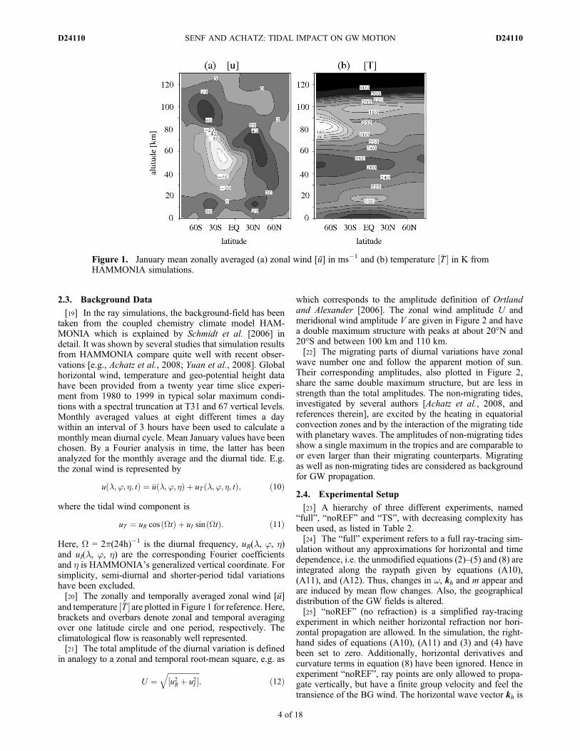
Here, W = 2p(24h)�1 is the diurnal frequency, uR(l, j, h)and uI(l, j, h) are the corresponding Fourier coefficientsand h is HAMMONIA’s generalized vertical coordinate. Forsimplicity, semi-diurnal and shorter-period tidal variationshave been excluded.[20] The zonally and temporally averaged zonal wind [ū]

and temperature �T½ �are plotted in Figure 1 for reference. Here,brackets and overbars denote zonal and temporal averagingover one latitude circle and one period, respectively. Theclimatological flow is reasonably well represented.[21] The total amplitude of the diurnal variation is defined

in analogy to a zonal and temporal root-mean square, e.g. as

U ¼ffiffiffiffiffiffiffiffiffiffiffiffiffiffiffiffiffiffiu2R þ u2I½ �

q; ð12Þ

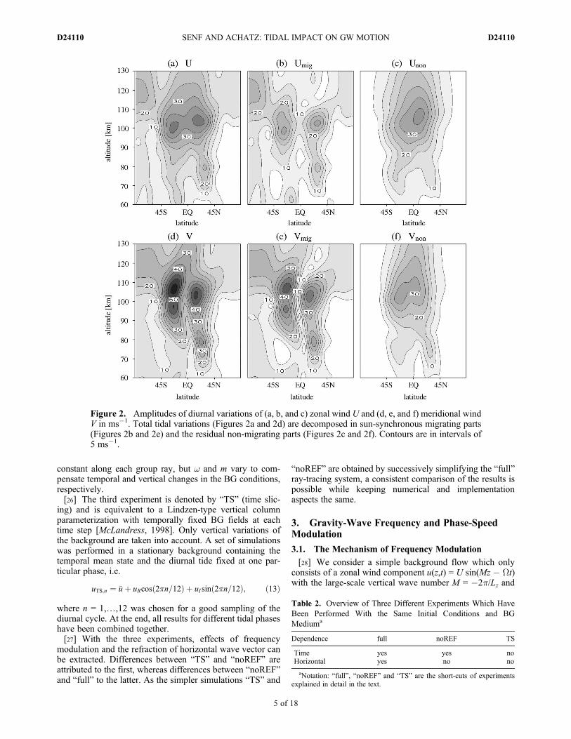
which corresponds to the amplitude definition of Ortlandand Alexander [2006]. The zonal wind amplitude U andmeridional wind amplitude V are given in Figure 2 and havea double maximum structure with peaks at about 20°N and20°S and between 100 km and 110 km.[22] The migrating parts of diurnal variations have zonal

wave number one and follow the apparent motion of sun.Their corresponding amplitudes, also plotted in Figure 2,share the same double maximum structure, but are less instrength than the total amplitudes. The non-migrating tides,investigated by several authors [Achatz et al., 2008, andreferences therein], are excited by the heating in equatorialconvection zones and by the interaction of the migrating tidewith planetary waves. The amplitudes of non-migrating tidesshow a single maximum in the tropics and are comparable toor even larger than their migrating counterparts. Migratingas well as non-migrating tides are considered as backgroundfor GW propagation.

2.4. Experimental Setup

[23] A hierarchy of three different experiments, named“full”, “noREF” and “TS”, with decreasing complexity hasbeen used, as listed in Table 2.[24] The “full” experiment refers to a full ray-tracing sim-

ulation without any approximations for horizontal and timedependence, i.e. the unmodified equations (2)–(5) and (8) areintegrated along the raypath given by equations (A10),(A11), and (A12). Thus, changes in w, kh and m appear andare induced by mean flow changes. Also, the geographicaldistribution of the GW fields is altered.[25] “noREF” (no refraction) is a simplified ray-tracing

experiment in which neither horizontal refraction nor hori-zontal propagation are allowed. In the simulation, the right-hand sides of equations (A10), (A11) and (3) and (4) havebeen set to zero. Additionally, horizontal derivatives andcurvature terms in equation (8) have been ignored. Hence inexperiment “noREF”, ray points are only allowed to propa-gate vertically, but have a finite group velocity and feel thetransience of the BG wind. The horizontal wave vector kh is

Figure 1. January mean zonally averaged (a) zonal wind [ū] in ms�1 and (b) temperature �T½ � in K fromHAMMONIA simulations.


4 of 18

constant along each group ray, but w and m vary to com-pensate temporal and vertical changes in the BG conditions,respectively.[26] The third experiment is denoted by “TS” (time slic-

ing) and is equivalent to a Lindzen-type vertical columnparameterization with temporally fixed BG fields at eachtime step [McLandress, 1998]. Only vertical variations ofthe background are taken into account. A set of simulationswas performed in a stationary background containing thetemporal mean state and the diurnal tide fixed at one par-ticular phase, i.e.

uTS;n ¼ �uþ uRcos 2pn=12ð Þ þ uI sin 2pn=12ð Þ; ð13Þ

where n = 1,…,12 was chosen for a good sampling of thediurnal cycle. At the end, all results for different tidal phaseshave been combined together.[27] With the three experiments, effects of frequency

modulation and the refraction of horizontal wave vector canbe extracted. Differences between “TS” and “noREF” areattributed to the first, whereas differences between “noREF”and “full” to the latter. As the simpler simulations “TS” and

“noREF” are obtained by successively simplifying the “full”ray-tracing system, a consistent comparison of the results ispossible while keeping numerical and implementationaspects the same.

3. Gravity-Wave Frequency and Phase-SpeedModulation

3.1. The Mechanism of Frequency Modulation

[28] We consider a simple background flow which onlyconsists of a zonal wind component u(z,t) = U sin(Mz � Wt)with the large-scale vertical wave number M = �2p/Lz and

Table 2. Overview of Three Different Experiments Which HaveBeen Performed With the Same Initial Conditions and BGMediuma

Dependence full noREF TS

Time yes yes noHorizontal yes no no

aNotation: “full”, “noREF” and “TS” are the short-cuts of experimentsexplained in detail in the text.

Figure 2. Amplitudes of diurnal variations of (a, b, and c) zonal wind U and (d, e, and f) meridional windV in ms�1. Total tidal variations (Figures 2a and 2d) are decomposed in sun-synchronous migrating parts(Figures 2b and 2e) and the residual non-migrating parts (Figures 2c and 2f). Contours are in intervals of5 ms�1.


5 of 18

vertical wavelength Lz [Broutman, 1984; Broutman andYoung, 1986; Eckermann and Marks, 1996]. For diurnaltides with M = �2p (30 km)�1 and W = 2p (1 day)�1, thephase progression C = W/M is downward and in the order of0.3 m/s. We assume that the wind amplitude U is zero at theground and slowly increases to a constant value above acertain altitude z0. Additionally, the thermodynamic BGstate is set to isothermal.[29] Two counter-propagating GW trains, i.e. propagating

in positive and negative zonal direction with zonal wavenumber k =�k0, are continuously emitted at ground with thephase velocities c = �c0. Then the ray-tracing equations (2)and (3) reduce to

dtw ¼ k∂tu; ð14Þ

dtk ¼ 0; ð15Þ

which can be combined to the ray equation for the zonalphase velocity c = w/k

dtc ¼ ∂tu: ð16Þ

From equation (16), we infer that a local tendency of BGwind is connected to a change of zonal phase velocity c alongthe ray. But as also shown by Eckermann and Marks [1996]and Walterscheid [2000], phase velocity changes arise onlydue to frequency changes. Above z0, u is monochromatic anda solution of the form c(z-Ct) can be found for whichequation (16) changes to

1þ cgzjCj

� �∂tc ¼ ∂tu: ð17Þ

Assuming small U, the ansatz

c ≈ �c0 þ dc sin Mz� Wtð Þ: ð18Þ

gives the phase velocity variation dc to the lowest order

dc ¼ U

1þ cgz;0jCj

; ð19Þ

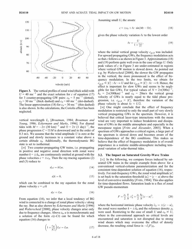
where the initial vertical group velocity cgz,0 was included.For upward propagating GWs, the frequency modulation actsso that c follows u as shown in Figure 3. Approximations (18)and (19) perform quite well even in the case of large U. Onlypeak values of c in Figure 3 are under-estimated in regionswhere vertical GW motion is slowed down. As pointed oute.g. by Walterscheid [2000], the slower the GW propagatesin the vertical, the more pronounced is the effect of fre-quency modulation. In the two limits, we obtain forcgz,0 ≪ |C| : dc → U and for cgz,0 ≫ |C| : dc → 0. Hence, theeffect is important for slow GWs and seems to be negli-gible for fast GWs. For typical values of N = 2p(300s)�1,kh = 2p(300km)�1 and c0 = 20m/s the vertical groupvelocity of GWs is nearly equal to the tidal phase pro-gression, i.e. cgz,0 ≈ |C|, therefore the variation of thephase velocity is about dc ≈ U/2.[30] One might conclude that the effect of frequency

modulation is restricted to only the small part of very slowlyvertical propagating GWs in the spectrum. However, it isbelieved that critical layer-type interactions with the meanwind are very important to induce breakdown and dissipa-tion of GWs in the middle atmosphere and especially in themesopause region [Fritts and Alexander, 2003]. When aspectrum of GWs approaches a critical region, a large part ofthe spectrum is slowed down and becomes aware of thetime-dependence of the BG conditions. This makes usbelieve that the effect of frequency modulation is of overallimportance in a realistic middle-atmosphere including tem-poral variation of solar-thermal tides.

3.2. The Impact on Saturated Gravity-Wave Trains

[31] In the following, we compare forces induced by sat-urated GW trains in the simple example from above: for aconventional vertical-column parameterization and for theconsistent time-dependent solution of equation (16), respec-tively. For mid-frequency GWs, the zonal wind amplitude |u′|is set back to the saturation threshold |us′ | = |c � u| above thelevel of convective instability [Fritts, 1984]. This also appliesfor time-dependent flows. Saturation leads to a flux of zonalGW pseudo-momentum

F ¼ rr2

k

Nc3h ¼

rr2

k0N

c� uð Þ3; ð20Þ

where the horizontal intrinsic phase velocity ch ¼ � c� uð Þ,the zonal wave number k = �k0 and the reference density rrwere used. Restricting to the case of small U and c0 ≫ U,where in the conventional approach no critical levels areencountered and saturation is not disrupted due to strongwind shears which may overcome the effect of densitydecrease, the resulting zonal force is �∂zF/rr.

Figure 3. The vertical profiles of zonal wind (thick solid) withU = 40 ms�1 and the exact solution for c of equation (17)for 3 counter-propagating GW pairs: c0 = 5 ms�1 (dotted),c0 = 30 ms�1 (thick dashed) and c0 = 60 ms�1 (dot-dashed).The linear approximation (18) for c0 = 30 ms�1 (thin dashed)is also shown. In the calculations, the Coriolis effect has beenneglected.


6 of 18

[32] In the conventional approach, the GW phase velocityis assumed is to be constant, i.e. c = �c0, and thus, thesaturation flux becomes

F�conv ¼

rr2

k0N

�c30 � 3c20Usin Mz� Wtð Þ þ…� �

; ð21Þ

where terms nonlinear in U are not given explicitly. Thediurnal force exerted on the mean flow due to the dampingof counter-propagating GWs is

fconv;T ¼ � 1

rr

∂∂z

Fþconv þ F�

conv

� � ð22Þ

¼ � 3c20Uk0N

1

HrsinFT �McosFT

� �ð23Þ

with the tidal phase FT = Mz � Wt and the density scaleheight Hr =� (∂zlnrr)�1. Terms nonlinear in U/c0 have beenneglected.[33] But, by taking realistic GW propagation into account,

the periodic change in the BG wind induces a modulation offrequency and hence zonal phase velocity (see equations (19)and (18)). This effect reduces the variation of the intrinsichorizontal phase velocity, saturation pseudo-momentumflux and hence the diurnal force due to GWs. Utilizingequation (18), we obtain for the diurnal force

fT ¼ fconv;T 1� dcU

� �ð24Þ

and recall that dc < U, which is ensured by equation (19).Therefore, the diurnal GW force fT is reduced due to phasevelocity variations compared to the conventional approach.Note also, that no critical layer is encountered for GWs inthe time-dependent approach. The localized deposition ofGW pseudo-momentum at the conventional critical layer issmoothed out by the effects of frequency modulation.

3.3. Vertical-Column Thinking and Phase-VelocityModulation in Realistic Flows

[34] As mentioned before, large-scale circulation modelsneed to apply GW parameterizations [McLandress, 1998].Horizontal gradients of the BG medium are neglected whichleads via equations (3) and (4) to a conserved horizontalwave number kh. Possibly of graver consequence, time-dependence of the transient large-scale motion is neglectedin the vertical column. GW trains are assumed to feel astationary background and adjust instantaneously to a givenwind field. In this sense, perturbations in the GW fieldpropagate infinitely fast to the levels above. The advectivetimescale, however, connected to the time which a part of aGW field vertically propagates can be in the order of a dayand longer. But, the scale-separation assumption is still ful-filled if the GW times scale �w�1 is significantly smallerthan a day. In equation (18), the ratio cgz,0/C can be inter-preted as ratio between BG timescale and GW advectivetimescale and directly affects the variation of GW phasevelocities and diurnal forces.

[35] The experience obtained from the vertical columnmodel has guided the conventional thinking of gravitywave - mean flow interaction. There, the horizontal phasevelocity of the GWs, ch, is assumed to be constant andcompared to the horizontal BG wind in GW direction,uh = u ⋅ kh/kh. The difference between both, i.e. the intrinsichorizontal phase velocity ch ¼ ch � uh , is to a goodapproximation direct proportional to the vertical GW length.When ch approaches its minimum, the vertical structure ofthe GW shrinks and turbulent diffusion becomes much moreeffective. The saturation momentum flux (20) is/ ch

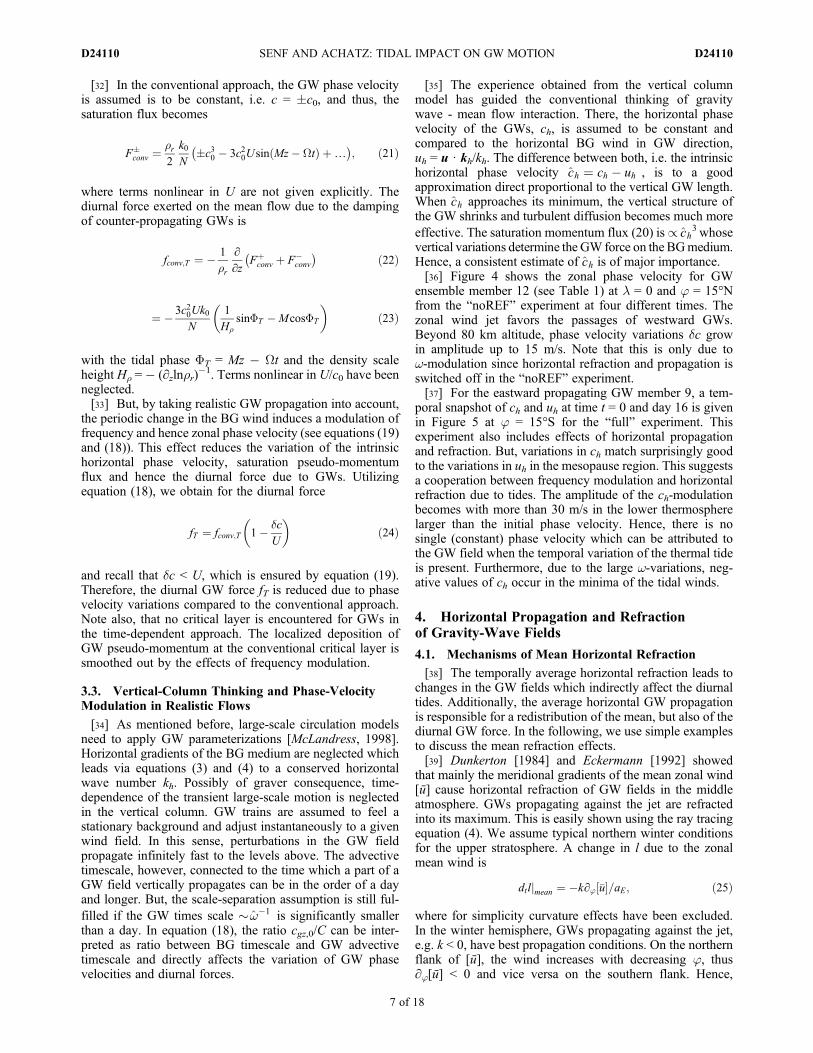
3 whosevertical variations determine the GW force on the BGmedium.Hence, a consistent estimate of ch is of major importance.[36] Figure 4 shows the zonal phase velocity for GW

ensemble member 12 (see Table 1) at l = 0 and j = 15°Nfrom the “noREF” experiment at four different times. Thezonal wind jet favors the passages of westward GWs.Beyond 80 km altitude, phase velocity variations dc growin amplitude up to 15 m/s. Note that this is only due tow-modulation since horizontal refraction and propagation isswitched off in the “noREF” experiment.[37] For the eastward propagating GW member 9, a tem-

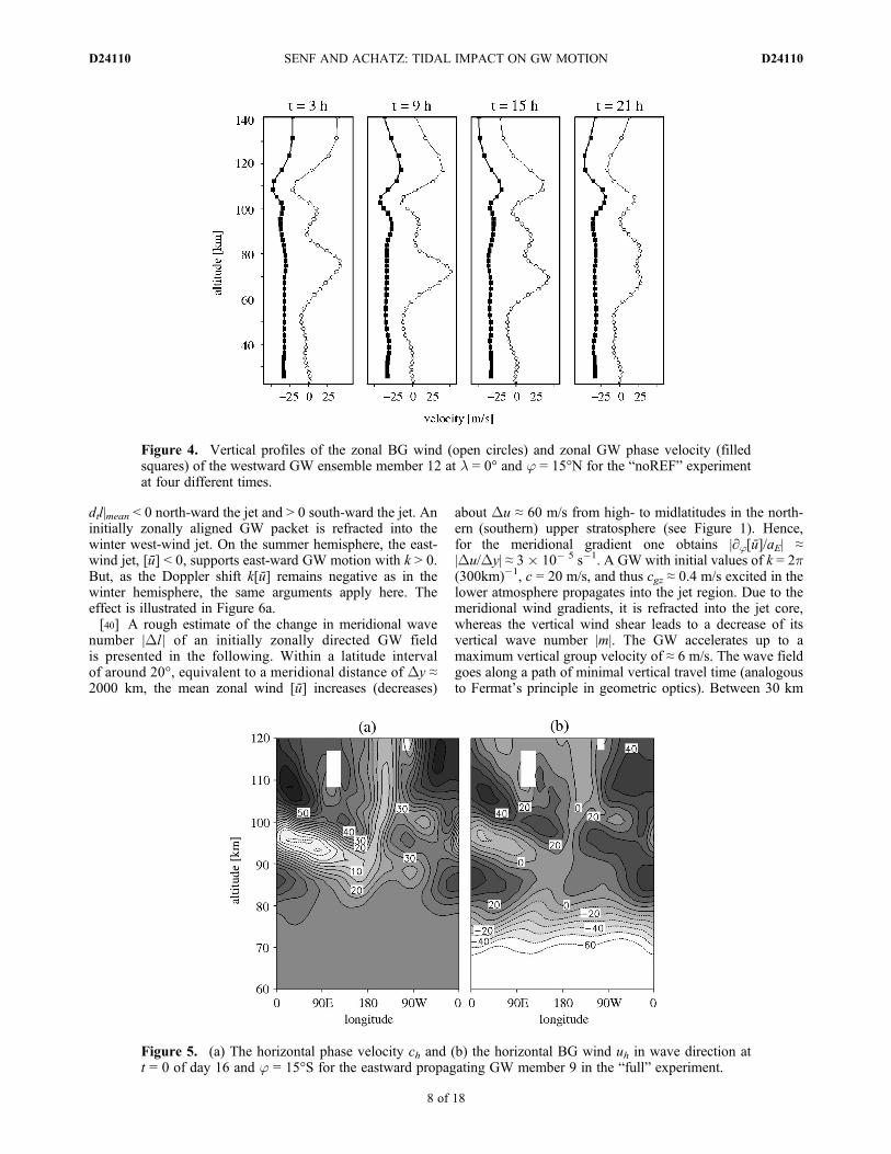
poral snapshot of ch and uh at time t = 0 and day 16 is givenin Figure 5 at j = 15°S for the “full” experiment. Thisexperiment also includes effects of horizontal propagationand refraction. But, variations in ch match surprisingly goodto the variations in uh in the mesopause region. This suggestsa cooperation between frequency modulation and horizontalrefraction due to tides. The amplitude of the ch-modulationbecomes with more than 30 m/s in the lower thermospherelarger than the initial phase velocity. Hence, there is nosingle (constant) phase velocity which can be attributed tothe GW field when the temporal variation of the thermal tideis present. Furthermore, due to the large w-variations, neg-ative values of ch occur in the minima of the tidal winds.

4. Horizontal Propagation and Refractionof Gravity-Wave Fields

4.1. Mechanisms of Mean Horizontal Refraction

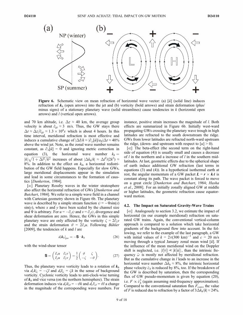
[38] The temporally average horizontal refraction leads tochanges in the GW fields which indirectly affect the diurnaltides. Additionally, the average horizontal GW propagationis responsible for a redistribution of the mean, but also of thediurnal GW force. In the following, we use simple examplesto discuss the mean refraction effects.[39] Dunkerton [1984] and Eckermann [1992] showed

that mainly the meridional gradients of the mean zonal wind[ū] cause horizontal refraction of GW fields in the middleatmosphere. GWs propagating against the jet are refractedinto its maximum. This is easily shown using the ray tracingequation (4). We assume typical northern winter conditionsfor the upper stratosphere. A change in l due to the zonalmean wind is

dtljmean ¼ �k∂j �u½ �=aE; ð25Þ

where for simplicity curvature effects have been excluded.In the winter hemisphere, GWs propagating against the jet,e.g. k < 0, have best propagation conditions. On the northernflank of [ū], the wind increases with decreasing j, thus∂j[ū] < 0 and vice versa on the southern flank. Hence,


7 of 18

dtl|mean < 0 north-ward the jet and > 0 south-ward the jet. Aninitially zonally aligned GW packet is refracted into thewinter west-wind jet. On the summer hemisphere, the east-wind jet, [ū] < 0, supports east-ward GW motion with k > 0.But, as the Doppler shift k[ū] remains negative as in thewinter hemisphere, the same arguments apply here. Theeffect is illustrated in Figure 6a.[40] A rough estimate of the change in meridional wave

number |Dl | of an initially zonally directed GW fieldis presented in the following. Within a latitude intervalof around 20°, equivalent to a meridional distance of Dy ≈2000 km, the mean zonal wind [ū] increases (decreases)

about Du ≈ 60 m/s from high- to midlatitudes in the north-ern (southern) upper stratosphere (see Figure 1). Hence,for the meridional gradient one obtains |∂j[ū]/aE| ≈|Du/Dy| ≈ 3 � 10� 5 s�1. A GW with initial values of k = 2p(300km)�1, c = 20 m/s, and thus cgz ≈ 0.4 m/s excited in thelower atmosphere propagates into the jet region. Due to themeridional wind gradients, it is refracted into the jet core,whereas the vertical wind shear leads to a decrease of itsvertical wave number |m|. The GW accelerates up to amaximum vertical group velocity of ≈ 6 m/s. The wave fieldgoes along a path of minimal vertical travel time (analogousto Fermat’s principle in geometric optics). Between 30 km

Figure 5. (a) The horizontal phase velocity ch and (b) the horizontal BG wind uh in wave direction att = 0 of day 16 and j = 15°S for the eastward propagating GW member 9 in the “full” experiment.

Figure 4. Vertical profiles of the zonal BG wind (open circles) and zonal GW phase velocity (filledsquares) of the westward GW ensemble member 12 at l = 0° and j = 15°N for the “noREF” experimentat four different times.


8 of 18

and 70 km altitude, i.e. Dz ≈ 40 km, the average groupvelocity is about cgz ≈ 3 m/s. Thus, the GW stays thereDt ≈ Dz=cgz ≈ 1:3� 104s which is about 4 hours. In thistime interval, meridional refraction is most effective andinduces a cumulative change of |Dl|/k ≈ |∂j[ū]/aE|Dt ≈ 40%above the wind jet. Note, as the zonal wave number remainsconstant, as ∂l[ū] = 0 and ignoring metric correction inequation (3), the horizontal wave number kh ¼jkj ffiffiffiffiffiffiffiffiffiffiffiffiffiffiffiffiffiffiffiffiffiffiffi

1þDl2=k2p

increases of about |Dkh/k| ≈ Dl2/(2k2) ≈8%. In addition to the effect on kh, a horizontal redistri-bution of the GW field happens. Especially for slow GWs,large meridional displacements appear in the simulationand lead in some circumstances to the formation of caus-tics [Dunkerton, 1984].[41] Planetary Rossby waves in the winter stratosphere

also affect the horizontal refraction of GWs [Dunkerton andButchart, 1984]. We refer to a simple wave field in a channelwith Cartesian geometry shown in Figure 6b. The planetarywave is described by a simple stream function y = �Ysin(x)sin(y), where x and y have been scaled by the channel sizeand Y is arbitrary. For u =�∂yy and v = ∂xy, divergence andshear deformation are zero. Hence, the GWs in this simpleplanetary wave are only affected by the vorticity z = 2∂xvand the strain deformation J = 2∂xu. Following Bühler[2009], the tendencies of k and l are

dtkhjpw ¼ �S ⋅ kh ð26Þ

with the wind-shear tensor

S ¼ ∂xu ∂xv∂yu ∂yv

� �¼ 1

2J z�z �J

� �: ð27Þ

Thus, the planetary wave vorticity leads to a rotation of khvia dtk|z = �zl and dtl|z = zk in the sense of backgroundvorticity. Cyclonic vorticity leads to anti-clock-wise turningof kh and vice versa (on the northern hemisphere). The straindeformation induces via dtk|J = �Jk and dt l |J = Jl a changein the magnitude of the corresponding wave numbers. For

instance, positive strain increases the magnitude of l. Botheffects are summarized in Figure 6b. Initially west-wardpropagating GWs crossing the planetary wave trough in highlatitudes are refracted to the south downstream the ridge.GWs from lower latitudes are refracted north-ward upstreamthe ridge, (down- and upstream with respect to [u] > 0).[42] The beta-effect (the second term on the right-hand

side of equation (4)) is usually small and causes a decreaseof l in the northern and a increase of l in the southern mid-latitudes. At last, geometric effects due to the spherical shapeof earth induce additional GW refraction (last terms inequations (3) and (4)). In a hypothetical isothermal earth atrest, the angular momentum of a GW packet L = r � kA isconstant along its path. The wave packet is forced to moveon a great circle [Dunkerton and Butchart, 1984; Hashaet al., 2008]. For an initially zonally aligned GW at middleor higher latitudes, the geometric refraction cause equator-ward motion.

4.2. The Impact on Saturated Gravity-Wave Trains

[43] Analogously to section 3.2, we estimate the impact ofhorizontal (in our example meridional) refraction on satu-rated GW trains. Again, the conventional vertical-columnapproach is compared to a solution which take horizontalgradients of the background flow into account. In the fol-lowing, we refer to the example of the last paragraph, a GWwith initial values of k = 2p(300 km)�1 and c = 20 m/smoving through a typical January zonal mean wind [ū]. Ifthe influence of the mean meridional wind on the Dopplershift is neglected, i.e. jl �v½ �j≪ jk �u½ �j , than the intrinsic fre-quency w is mostly not affected by meridional refraction.But as the cumulative change in l leads to an increase in thehorizontal wave number Dkh ≈ 8%, the intrinsic horizontalphase velocity ch is reduced by 8%, too. If the breakdown ofthe GW is described by saturation, then the correspondingflux of GW pseudo-momentum is given by equation (20),i.e. F / c3h (again assuming mid-frequency approximation).Compared to the conventional saturation flux Fconv, the valueof F is reduced due to refraction by a factor of 3Dkh/|k| ≈ 24%.

Figure 6. Schematic view on mean refraction of horizontal wave vector: (a) [ū] (solid line) inducesrefraction of kh (open arrows) into the jet and (b) vorticity (bold arrows) and strain deformation (plus/minus signs) of a stationary planetary wave (solid streamlines) cause tendencies in k (horizontal openarrows) and l (vertical open arrows).


9 of 18

Therefore, if the vertical dependence of this additional factoris ignored, the real zonal force fl is also diminished byhorizontal refraction compared to the force fconv,l calculatedwithin the vertical-column approach, i.e.

fl ¼ fconv;l 1� 3Dkhkh

� �: ð28Þ

The force reduction due to horizontal gradients is mainly atemporally average effect, but reduces the diurnal GW forceas well.

4.3. Horizontal Refraction in Realistic Flows

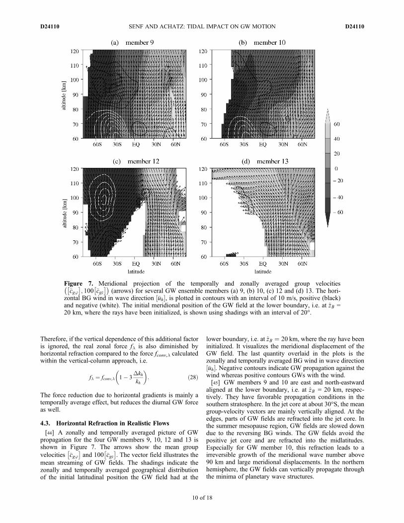
[44] A zonally and temporally averaged picture of GWpropagation for the four GW members 9, 10, 12 and 13 isshown in Figure 7. The arrows show the mean groupvelocities �cgj

� �and 100 �cgz

� �. The vector field illustrates the

mean streaming of GW fields. The shadings indicate thezonally and temporally averaged geographical distributionof the initial latitudinal position the GW field had at the

lower boundary, i.e. at zB ¼ 20 km, where the ray have beeninitialized. It visualizes the meridional displacement of theGW field. The last quantity overlaid in the plots is thezonally and temporally averaged BG wind in wave direction�uh½ �. Negative contours indicate GW propagation against thewind whereas positive contours GWs with the wind.[45] GW members 9 and 10 are east and north-eastward

aligned at the lower boundary, i.e. at zB = 20 km, respec-tively. They have favorable propagation conditions in thesouthern stratosphere. In the jet core at about 30°S, the meangroup-velocity vectors are mainly vertically aligned. At theedges, parts of GW fields are refracted into the jet core. Inthe summer mesopause region, GW fields are slowed downdue to the reversing BG winds. The GW fields avoid thepositive jet core and are refracted into the midlatitudes.Especially for GW member 10, this refraction leads to airreversible growth of the meridional wave number above90 km and large meridional displacements. In the northernhemisphere, the GW fields can vertically propagate throughthe minima of planetary wave structures.

Figure 7. Meridional projection of the temporally and zonally averaged group velocities�cgj� �

; 100 �cgz� ��

(arrows) for several GW ensemble members (a) 9, (b) 10, (c) 12 and (d) 13. The hori-zontal BG wind in wave direction �uh½ �, is plotted in contours with an interval of 10 m/s, positive (black)and negative (white). The initial meridional position of the GW field at the lower boundary, i.e. at zB =20 km, where the rays have been initialized, is shown using shadings with an interval of 20°.


10 of 18

[46] GW members 12 and 13 are west and south-westwardaligned at the lower boundary, i.e. at zB = 20 km, respec-tively. The westerly wind vortex of the northern winterhemisphere provides most favorable propagation conditions.In the jet core, the group velocities are mainly vertical. Atthe wind reversal, GW fields are refracted into meridionaldirection. For GW member 13, the mean latitude positionsare interchanged in the lower thermosphere. Parts of the GWfield initially from the northern midlatitudes have movedsouth-ward to the equatorial region and even to the southernhemisphere, whereas parts of the GW field initially from thesubtropics have propagated north-wards. As discussedbefore, due to the modulation of stratospheric winds byplanetary waves zonally dependent waveguides develop.The easterly wind jet in the southern hemisphere mainlyprohibits propagation of GW member 12 and 13. Interest-ingly, some chance exists for parts of the high-latitude GWfield to circumvent the jet core (GW member 12). Above thecritical jet GW fields are refracted southward and spreadover a large horizontal domain. The considerable horizontalexpansion of GW fields, as seen for GW member 12 at e.g.100 km and between 80° and 10°N as well as GW member13 above 110 km and between 80°S and 30°N, also influ-ences the amplitudes of the GW field via equation (8). Thecorresponding change in GW amplitudes is not incorporatedin most previous ray-tracing work [Marks and Eckermann,1995; Hasha et al., 2008; Song and Chun, 2008] whichcommonly apply the assumption of a constant vertical fluxFA = cgzA of wave action density A.[47] The median meridional displacement for GW mem-

ber 9 and 12 remains around zero in the MLT, but largedisplacements up to 50° are also possible. For member 10and 13, median displacement of 26° and �27° occur,respectively, but its distribution is broad with maximumvalues up to 100°. Hence, some parts of the GW fields areinterchanged between both hemispheres.

5. Gravity-Wave Forces on the Tide

5.1. Mean Gravity-Wave Forces

[48] Before investigating the periodic GW forces, whichare one major focus of this study, changes in the temporallymean GW force are inspected. As discussed e.g. by Andrewset al. [1987], the relevant GW forcing of the mean flow, inour case temporally averaged flow plus diurnal tides, isgiven by the divergence of the GW pseudo-momentum fluxrather than the GW momentum flux itself. The main differ-ence between both arise for slowly vertically propagating,inertia-gravity waves. These waves produce a Stokes driftwhich is counterbalanced by an Eulerian mean flow locallyattached to the waves [Bühler, 2009]. Hence, some parts ofthe force inferred from the divergence of momentum flux areneeded to sustain the local Eulerian circulation and do notchange the BG conditions. The vertical flux of zonal pseudo-momentum is [Fritts and Alexander, 2003]

FP;l ¼ cgzkA ¼ rr⟨u′w′⟩ 1� f 2

w2

� �; ð29Þ

where the prime denotes GW perturbations which are aver-aged over reasonable GW scales via the bracket operator.

Therefore, the wave stress on the (Lagrangian) mean flow isreduced by a factor of f 2 over w2.[49] In neglecting horizontal variations in the GW fields,

the horizontal force due to GW stresses is expressed as[Fritts and Alexander, 2003]

fh ≈� 1

rr∂z cgzkhA� �

: ð30Þ

As we are interested in the effects of horizontal inhomoge-neities in the BG conditions on the diurnal GW force, themore complete form [Grimshaw, 1975]

fh ¼ � 1

rrr ⋅ cgkhA

� � ð31Þ

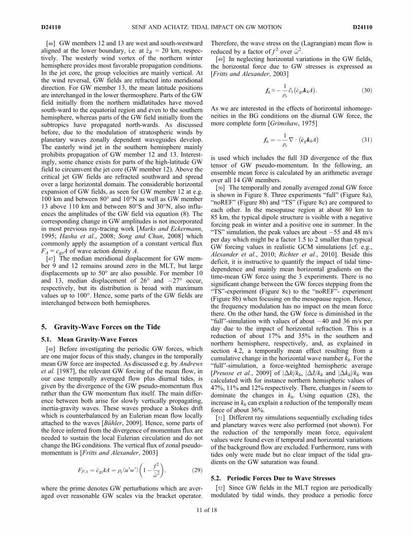
is used which includes the full 3D divergence of the fluxtensor of GW pseudo-momentum. In the following, anensemble mean force is calculated by an arithmetic averageover all 14 GW members.[50] The temporally and zonally averaged zonal GW force

is shown in Figure 8. Three experiments “full” (Figure 8a),“noREF” (Figure 8b) and “TS” (Figure 8c) are compared toeach other. In the mesopause region at about 80 km to85 km, the typical dipole structure is visible with a negativeforcing peak in winter and a positive one in summer. In the“TS” simulation, the peak values are about �55 and 48 m/sper day which might be a factor 1.5 to 2 smaller than typicalGW forcing values in realistic GCM simulations [cf. e.g.,Alexander et al., 2010; Richter et al., 2010]. Beside thisdeficit, it is instructive to quantify the impact of tidal time-dependence and mainly mean horizontal gradients on thetime-mean GW force using the 3 experiments. There is nosignificant change between the GW forces stepping from the“TS”-experiment (Figure 8c) to the “noREF”- experiment(Figure 8b) when focusing on the mesopause region. Hence,the frequency modulation has no impact on the mean forcethere. On the other hand, the GW force is diminished in the“full”-simulation with values of about �40 and 36 m/s perday due to the impact of horizontal refraction. This is areduction of about 17% and 35% in the southern andnorthern hemisphere, respectively, and, as explained insection 4.2, a temporally mean effect resulting from acumulative change in the horizontal wave number kh. For the“full”-simulation, a force-weighted hemispheric average[Preusse et al., 2009] of |Dk|/kh, |Dl|/kh and |Dkh|/kh wascalculated with for instance northern hemispheric values of47%, 11% and 12% respectively. There, changes in l seem todominate the changes in kh. Using equation (28), theincrease in kh can explain a reduction of the temporally meanforce of about 36%.[51] Different ray simulations sequentially excluding tides

and planetary waves were also performed (not shown). Forthe reduction of the temporally mean force, equivalentvalues were found even if temporal and horizontal variationsof the background flow are excluded. Furthermore, runs withtides only were made but no clear impact of the tidal gra-dients on the GW saturation was found.

5.2. Periodic Forces Due to Wave Stresses

[52] Since GW fields in the MLT region are periodicallymodulated by tidal winds, they produce a periodic force


11 of 18

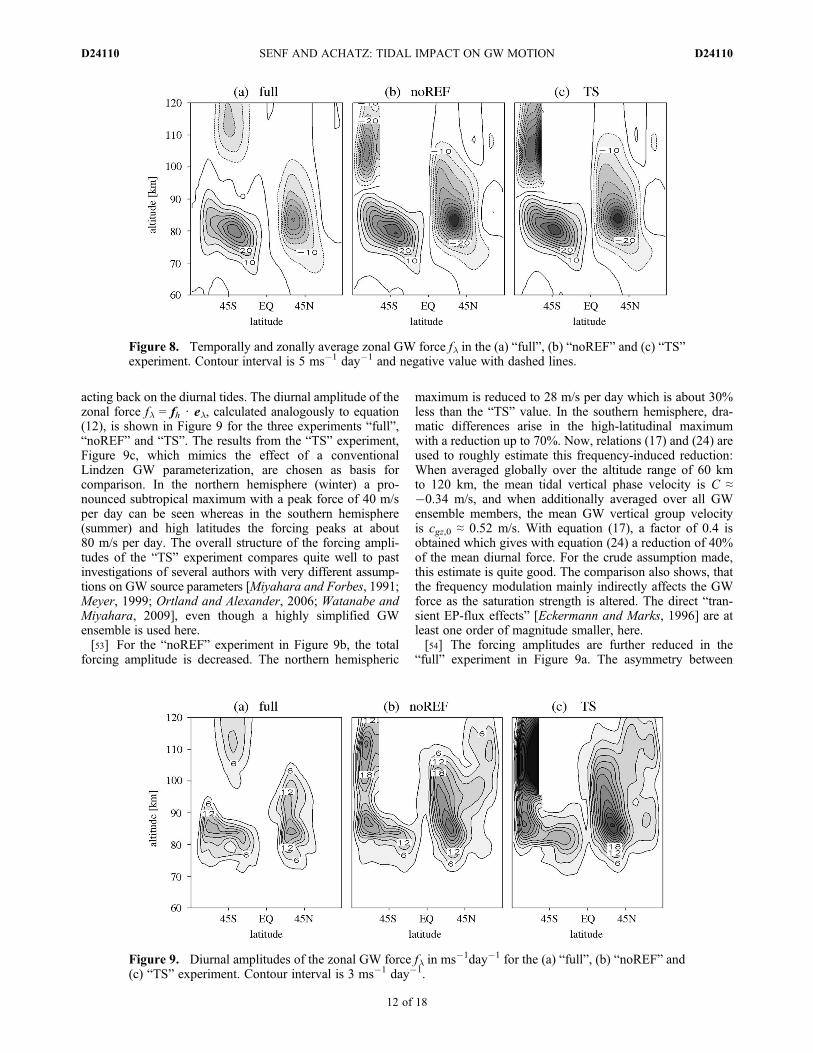
acting back on the diurnal tides. The diurnal amplitude of thezonal force fl = fh ⋅ el, calculated analogously to equation(12), is shown in Figure 9 for the three experiments “full”,“noREF” and “TS”. The results from the “TS” experiment,Figure 9c, which mimics the effect of a conventionalLindzen GW parameterization, are chosen as basis forcomparison. In the northern hemisphere (winter) a pro-nounced subtropical maximum with a peak force of 40 m/sper day can be seen whereas in the southern hemisphere(summer) and high latitudes the forcing peaks at about80 m/s per day. The overall structure of the forcing ampli-tudes of the “TS” experiment compares quite well to pastinvestigations of several authors with very different assump-tions on GW source parameters [Miyahara and Forbes, 1991;Meyer, 1999; Ortland and Alexander, 2006; Watanabe andMiyahara, 2009], even though a highly simplified GWensemble is used here.[53] For the “noREF” experiment in Figure 9b, the total

forcing amplitude is decreased. The northern hemispheric

maximum is reduced to 28 m/s per day which is about 30%less than the “TS” value. In the southern hemisphere, dra-matic differences arise in the high-latitudinal maximumwith a reduction up to 70%. Now, relations (17) and (24) areused to roughly estimate this frequency-induced reduction:When averaged globally over the altitude range of 60 kmto 120 km, the mean tidal vertical phase velocity is C ≈�0.34 m/s, and when additionally averaged over all GWensemble members, the mean GW vertical group velocityis cgz,0 ≈ 0.52 m/s. With equation (17), a factor of 0.4 isobtained which gives with equation (24) a reduction of 40%of the mean diurnal force. For the crude assumption made,this estimate is quite good. The comparison also shows, thatthe frequency modulation mainly indirectly affects the GWforce as the saturation strength is altered. The direct “tran-sient EP-flux effects” [Eckermann and Marks, 1996] are atleast one order of magnitude smaller, here.[54] The forcing amplitudes are further reduced in the

“full” experiment in Figure 9a. The asymmetry between

Figure 9. Diurnal amplitudes of the zonal GW force fl in ms�1day�1 for the (a) “full”, (b) “noREF” and(c) “TS” experiment. Contour interval is 3 ms�1 day�1.

Figure 8. Temporally and zonally average zonal GW force fl in the (a) “full”, (b) “noREF” and (c) “TS”experiment. Contour interval is 5 ms�1 day�1 and negative value with dashed lines.


12 of 18

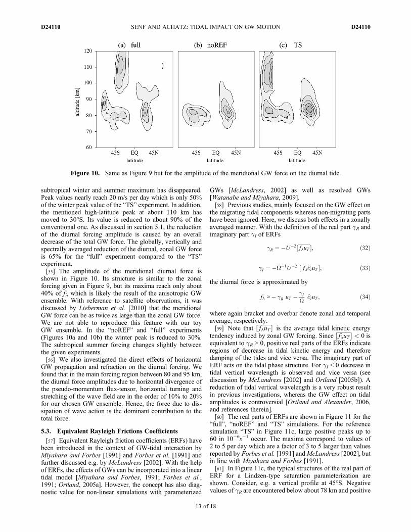
subtropical winter and summer maximum has disappeared.Peak values nearly reach 20 m/s per day which is only 50%of the winter peak value of the “TS” experiment. In addition,the mentioned high-latitude peak at about 110 km hasmoved to 30°S. Its value is reduced to about 90% of theconventional one. As discussed in section 5.1, the reductionof the diurnal forcing amplitude is caused by an overalldecrease of the total GW force. The globally, vertically andspectrally averaged reduction of the diurnal, zonal GW forceis 65% for the “full” experiment compared to the “TS”experiment.[55] The amplitude of the meridional diurnal force is

shown in Figure 10. Its structure is similar to the zonalforcing given in Figure 9, but its maxima reach only about40% of fl which is likely the result of the anisotropic GWensemble. With reference to satellite observations, it wasdiscussed by Lieberman et al. [2010] that the meridionalGW force can be as twice as large than the zonal GW force.We are not able to reproduce this feature with our toyGW ensemble. In the “noREF” and “full” experiments(Figures 10a and 10b) the winter peak is reduced to 30%.The subtropical summer forcing changes slightly betweenthe given experiments.[56] We also investigated the direct effects of horizontal

GW propagation and refraction on the diurnal forcing. Wefound that in the main forcing region between 80 and 95 km,the diurnal force amplitudes due to horizontal divergence ofthe pseudo-momentum flux-tensor, horizontal turning andstretching of the wave field are in the order of 10% to 20%for our chosen GW ensemble. Hence, the force due to dis-sipation of wave action is the dominant contribution to thetotal force.

5.3. Equivalent Rayleigh Frictions Coefficients

[57] Equivalent Rayleigh friction coefficients (ERFs) havebeen introduced in the context of GW-tidal interaction byMiyahara and Forbes [1991] and Forbes et al. [1991] andfurther discussed e.g. by McLandress [2002]. With the helpof ERFs, the effects of GWs can be incorporated into a lineartidal model [Miyahara and Forbes, 1991; Forbes et al.,1991; Ortland, 2005a]. However, the concept has also diag-nostic value for non-linear simulations with parameterized

GWs [McLandress, 2002] as well as resolved GWs[Watanabe and Miyahara, 2009].[58] Previous studies, mainly focused on the GW effect on

the migrating tidal components whereas non-migrating partshave been ignored. Here, we discuss both effects in a zonallyaveraged manner. With the definition of the real part gR andimaginary part gI of ERFs

gR ¼ �U�2�fluT �;½ ð32Þ

gI ¼ �W�1U�2�fl∂tuT �;½ ð33Þ

the diurnal force is approximated by

fl ≈� gR uT � gIW

∂tuT ; ð34Þ

where again bracket and overbar denote zonal and temporalaverage, respectively.[59] Note that�fluT �½ is the average tidal kinetic energy

tendency induced by zonal GW forcing. Since�fluT � < 0½ isequivalent to gR > 0, positive real parts of the ERFs indicateregions of decrease in tidal kinetic energy and thereforedamping of the tides and vice versa. The imaginary part ofERF acts on the tidal phase structure. For gI < 0 decrease intidal vertical wavelength is observed and vice versa (seediscussion by McLandress [2002] and Ortland [2005b]). Areduction of tidal vertical wavelength is a very robust resultin previous investigations, whereas the GW effect on tidalamplitudes is controversial [Ortland and Alexander, 2006,and references therein].[60] The real parts of ERFs are shown in Figure 11 for the

“full”, “noREF” and “TS” simulations. For the referencesimulation “TS” in Figure 11c, large positive peaks up to60 in 10�6s�1 occur. The maxima correspond to values of2 to 5 per day which are a factor of 3 to 5 larger than valuesreported by Forbes et al. [1991] andMcLandress [2002], butin line with Miyahara and Forbes [1991].[61] In Figure 11c, the typical structures of the real part of

ERF for a Lindzen-type saturation parameterization areshown. Consider, e.g. a vertical profile at 45°S. Negativevalues of gR are encountered below about 78 km and positive

Figure 10. Same as Figure 9 but for the amplitude of the meridional GW force on the diurnal tide.


13 of 18

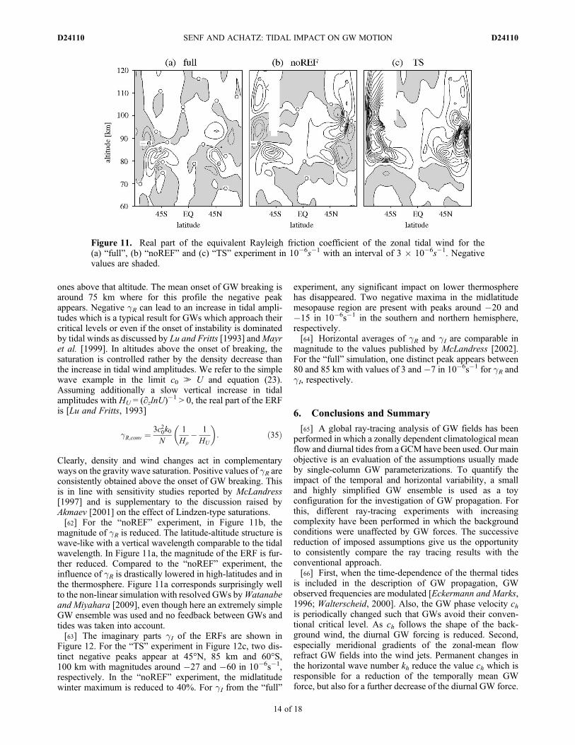
ones above that altitude. The mean onset of GW breaking isaround 75 km where for this profile the negative peakappears. Negative gR can lead to an increase in tidal ampli-tudes which is a typical result for GWs which approach theircritical levels or even if the onset of instability is dominatedby tidal winds as discussed by Lu and Fritts [1993] andMayret al. [1999]. In altitudes above the onset of breaking, thesaturation is controlled rather by the density decrease thanthe increase in tidal wind amplitudes. We refer to the simplewave example in the limit c0 ≫ U and equation (23).Assuming additionally a slow vertical increase in tidalamplitudes with HU = (∂zlnU)�1 > 0, the real part of the ERFis [Lu and Fritts, 1993]

gR;conv ¼3c20k0N

1

Hr� 1

HU

� �: ð35Þ

Clearly, density and wind changes act in complementaryways on the gravity wave saturation. Positive values of gR areconsistently obtained above the onset of GW breaking. Thisis in line with sensitivity studies reported by McLandress[1997] and is supplementary to the discussion raised byAkmaev [2001] on the effect of Lindzen-type saturations.[62] For the “noREF” experiment, in Figure 11b, the

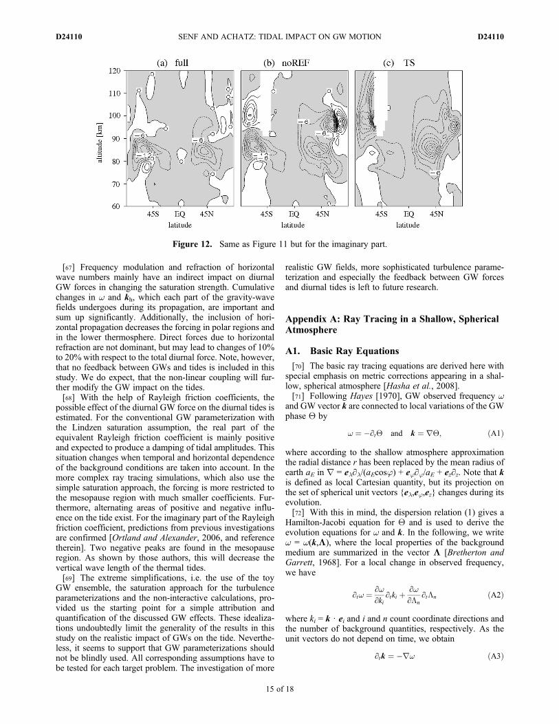
magnitude of gR is reduced. The latitude-altitude structure iswave-like with a vertical wavelength comparable to the tidalwavelength. In Figure 11a, the magnitude of the ERF is fur-ther reduced. Compared to the “noREF” experiment, theinfluence of gR is drastically lowered in high-latitudes and inthe thermosphere. Figure 11a corresponds surprisingly wellto the non-linear simulation with resolved GWs byWatanabeand Miyahara [2009], even though here an extremely simpleGW ensemble was used and no feedback between GWs andtides was taken into account.[63] The imaginary parts gI of the ERFs are shown in

Figure 12. For the “TS” experiment in Figure 12c, two dis-tinct negative peaks appear at 45°N, 85 km and 60°S,100 km with magnitudes around �27 and �60 in 10�6s�1,respectively. In the “noREF” experiment, the midlatitudewinter maximum is reduced to 40%. For gI from the “full”

experiment, any significant impact on lower thermospherehas disappeared. Two negative maxima in the midlatitudemesopause region are present with peaks around �20 and�15 in 10�6s�1 in the southern and northern hemisphere,respectively.[64] Horizontal averages of gR and gI are comparable in

magnitude to the values published by McLandress [2002].For the “full” simulation, one distinct peak appears between80 and 85 km with values of 3 and �7 in 10�6s�1 for gR andgI, respectively.

6. Conclusions and Summary

[65] A global ray-tracing analysis of GW fields has beenperformed in which a zonally dependent climatological meanflow and diurnal tides from a GCM have been used. Our mainobjective is an evaluation of the assumptions usually madeby single-column GW parameterizations. To quantify theimpact of the temporal and horizontal variability, a smalland highly simplified GW ensemble is used as a toyconfiguration for the investigation of GW propagation. Forthis, different ray-tracing experiments with increasingcomplexity have been performed in which the backgroundconditions were unaffected by GW forces. The successivereduction of imposed assumptions give us the opportunityto consistently compare the ray tracing results with theconventional approach.[66] First, when the time-dependence of the thermal tides

is included in the description of GW propagation, GWobserved frequencies are modulated [Eckermann and Marks,1996; Walterscheid, 2000]. Also, the GW phase velocity chis periodically changed such that GWs avoid their conven-tional critical level. As ch follows the shape of the back-ground wind, the diurnal GW forcing is reduced. Second,especially meridional gradients of the zonal-mean flowrefract GW fields into the wind jets. Permanent changes inthe horizontal wave number kh reduce the value ch which isresponsible for a reduction of the temporally mean GWforce, but also for a further decrease of the diurnal GW force.

Figure 11. Real part of the equivalent Rayleigh friction coefficient of the zonal tidal wind for the(a) “full”, (b) “noREF” and (c) “TS” experiment in 10�6s�1 with an interval of 3 � 10�6s�1. Negativevalues are shaded.


14 of 18

[67] Frequency modulation and refraction of horizontalwave numbers mainly have an indirect impact on diurnalGW forces in changing the saturation strength. Cumulativechanges in w and kh, which each part of the gravity-wavefields undergoes during its propagation, are important andsum up significantly. Additionally, the inclusion of hori-zontal propagation decreases the forcing in polar regions andin the lower thermosphere. Direct forces due to horizontalrefraction are not dominant, but may lead to changes of 10%to 20% with respect to the total diurnal force. Note, however,that no feedback between GWs and tides is included in thisstudy. We do expect, that the non-linear coupling will fur-ther modify the GW impact on the tides.[68] With the help of Rayleigh friction coefficients, the

possible effect of the diurnal GW force on the diurnal tides isestimated. For the conventional GW parameterization withthe Lindzen saturation assumption, the real part of theequivalent Rayleigh friction coefficient is mainly positiveand expected to produce a damping of tidal amplitudes. Thissituation changes when temporal and horizontal dependenceof the background conditions are taken into account. In themore complex ray tracing simulations, which also use thesimple saturation approach, the forcing is more restricted tothe mesopause region with much smaller coefficients. Fur-thermore, alternating areas of positive and negative influ-ence on the tide exist. For the imaginary part of the Rayleighfriction coefficient, predictions from previous investigationsare confirmed [Ortland and Alexander, 2006, and referencetherein]. Two negative peaks are found in the mesopauseregion. As shown by those authors, this will decrease thevertical wave length of the thermal tides.[69] The extreme simplifications, i.e. the use of the toy

GW ensemble, the saturation approach for the turbulenceparameterizations and the non-interactive calculations, pro-vided us the starting point for a simple attribution andquantification of the discussed GW effects. These idealiza-tions undoubtedly limit the generality of the results in thisstudy on the realistic impact of GWs on the tide. Neverthe-less, it seems to support that GW parameterizations shouldnot be blindly used. All corresponding assumptions have tobe tested for each target problem. The investigation of more

realistic GW fields, more sophisticated turbulence parame-terization and especially the feedback between GW forcesand diurnal tides is left to future research.

Appendix A: Ray Tracing in a Shallow, SphericalAtmosphere

A1. Basic Ray Equations

[70] The basic ray tracing equations are derived here withspecial emphasis on metric corrections appearing in a shal-low, spherical atmosphere [Hasha et al., 2008].[71] Following Hayes [1970], GW observed frequency w

and GW vector k are connected to local variations of the GWphase Q by

w ¼ �∂tQ and k ¼ rQ; ðA1Þ

where according to the shallow atmosphere approximationthe radial distance r has been replaced by the mean radius ofearth aE in r = el∂l/(aEcosj) + ej∂j/aE + ez∂z. Note that kis defined as local Cartesian quantity, but its projection onthe set of spherical unit vectors {el,ej,ez} changes during itsevolution.[72] With this in mind, the dispersion relation (1) gives a

Hamilton-Jacobi equation for Q and is used to derive theevolution equations for w and k. In the following, we writew = w(k,L), where the local properties of the backgroundmedium are summarized in the vector L [Bretherton andGarrett, 1968]. For a local change in observed frequency,we have

∂tw ¼ ∂w∂ki

∂tki þ ∂w∂Ln

∂tLn ðA2Þ

where ki = k ⋅ ei and i and n count coordinate directions andthe number of background quantities, respectively. As theunit vectors do not depend on time, we obtain

∂tk ¼ �rw ðA3Þ

Figure 12. Same as Figure 11 but for the imaginary part.


15 of 18

and

dtw ¼ ∂w∂Ln

∂tLn; ðA4Þ

where the group velocity is cg = (∂kiw)ei, and the advectivederivative along a ray dt = ∂t + cg ⋅ r.[73] For the GW vector k, the same procedure applies and

using equation (A3) gives

∂tk ¼ � ∂w∂ki

rki � ∂w∂Ln

rLn: ðA5Þ

Next we show that the term cgirki can be rewritten as anadvective derivative supplemented by metric corrections.We get

cgirki ¼ cgir k ⋅ eið Þ ¼ rk ⋅ cg þ cgirei ⋅ k:

Sincerk =rrQ is a symmetric tensor of second order, i.e.rk = (rk)T, we obtain rk ⋅ cg = cg ⋅ rk. Applying theprojection k = kiei, once again, we arrive at

cgirki ¼ cg ⋅rki� �

ei þ cg ⋅reiki þ cgirei ⋅ k¼ cg ⋅rki

� �ei þ cg ⋅ rei � reið ÞT

ki;

where in the last line r(ei ⋅ ej) = 0 was used. Hence, the rayequations for the wave numbers ki are

dtkið Þei ¼ � ∂w∂Ln

rLn � cg ⋅ rei � reð ÞT

ki; ðA6Þ

which are valid for quite general coordinate systems [Hashaet al., 2008].[74] As before, the shallow atmosphere approximation

will be used in which vertical derivatives of all unit vectorsand all derivatives of the outward pointing unit vector ez areneglected. Thus, only the convergence of meridians is takeninto account via

rel ¼ tanjaE

elej and rej ¼ � tanjaE

elel: ðA7Þ

Using additionally

∂w∂u

¼ k;∂w∂v

¼ l;∂w∂f

¼ fm2

wjkj2 and∂w∂N

¼ Nk2hwjkj2 ; ðA8Þ

the ray equations (2)–(5) are obtained. Furthermore, rewrit-ing ui = u ⋅ ei in equations (2)–(5) led to the change cg → cgin the corresponding metric corrections.

A2. RAPAGI: The Numerical Implementation

[75] The RAy parameterization of Gravity wave Impacts(RAPAGI) is a fast numerical model which allows to solvethe ray tracing equations on a spherical globe. For the directuse of GCM data, it is favorable to identify the position x ofthe wave parcel in spherical coordinates l, j and an altitudezwhich will be the globally averaged geo-potential height onsurfaces of the vertical hybrid coordinate h. As each changeof z along the ray is expressed as

dtz ¼ ∂tzþ dtlð Þ∂lzþ dtjð Þ∂jzþ dtzð Þ∂z z; ðA9Þ

the evolution of a ray point is given by

dtl ¼ cglaEcosj

; ðA10Þ

dtj ¼ cgyaE

; ðA11Þ

dtz ¼ cgz � ∂tz� cg⋅rhz

∂z z; ðA12Þ

where the components of group velocity cg are

cgl ¼ uþ k

jkj2N2 � w2

w; ðA13Þ

cgj ¼ vþ l

jkj2N 2 � w2

w; ðA14Þ

cgz ¼ � m

jkj2w2 � f 2

w: ðA15Þ

This facilitates inter-model communication. The partialderivatives in equations (2)–(5) are given in a coordinatesystem with geometric altitude z, while these quantities areusually calculated from the large-scale flow in generalizedcoordinates l;j; z hð Þf g . The transformation between bothwas taken into account in our ray tracing simulations.[76] The time-integration of equations (2)–(5) is done in

two stages. First, an integration estimate {wn+1* ,kn+1* } fortime (n + 1)Dt is obtained using the Heun scheme witha fixed time step of Dt = 5 min for which convergencehas been verified. Second, an optimization technique is usedto adaptively change all ray properties till the dispersionrelation is retained. For bi ≪ 1, the corrected estimateswn+1 =wn + Dw(1 + b0) with Dw = wn+1* � wn and ki,n+1 =ki,n + Dki(1 + bi) with Dki = ki,n+1* � ki,n fulfill dispersionrelation (1). In the optimization progress, the functional

G ¼ 1

2

X3i¼0

b2i þ b w knþ1;Lnþ1ð Þ � wnþ1ð Þ ðA16Þ

is minimized. The variation of G with respect to bi givesb0 ¼ bDw and bi ¼ �bcgi;nþ1Dki for i > 0. Inserted in thedispersion relation, a non-linear equation for the Lagrangianmultiplier b results which is solved numerically via theNewton method. Therefore, in the two-stage scheme, theadditional information gained by the w-equation (2) is usedto correct numerical errors and stabilize the implementedmethod.[77] Each time step, new ray points are injected at zB =

20 km and after a warming time of one day most of themodel domain, in which GW propagation is possible, isfilled with ray points. Furthermore, ray points are randomlyremoved when their number exceeds 32 in a grid box of thelarge-scale model.[78] All BG quantities are interpolated to the ray position

via a linear polygonal interpolation. Furthermore, a distance-weighted interpolation and running median average is usedto obtain smooth GW properties on the large-scale mesh.


16 of 18

Especially, for the forcing term (9), the group velocity cg issmoothly interpolated to the large-scale mesh. Derivatives ofcg were calculated using centered differences and tnon isobtained via equation (9). In the last step, tnon is interpolatedback to the ray position. Within this pragmatic approach,caustics appearing at ray crossings, are smoothed out and thecorresponding wave action density remains finite, there.This might be interpreted as caustic correction, for which, toour current knowledge, no efficient method for full time-dependent 3D flows exists.[79] For ray integrations, no explicit test of WKB validity

is performed. Only rays which cross the extreme thresholdsof 100 km vertical wavelength and 10 days intrinsic periodare removed from the model run. As noted by Sartelet[2003], ray theory performs remarkably good even if thescale separation assumption is not fulfilled.

[80] Acknowledgments. The authors would like to thank ErichBecker for fruitful and inspiring discussions and Hauke Schmidt fromMPI Hamburg for providing the set of HAMMONIA data. Furthermore,we thank three anonymous reviewers whose suggestions led to considerableimprovements. U.A. thanks Deutsche Forschungsgemeinschaft for partialsupport through the MetStröm Priority Research Program (SPP 1276),and through grant Ac 71/4-1. U.A. and F.S. thank Deutsche Forschungsge-meinschaft for partial support through the CAWSES Priority ResearchProgram (SPP 1176), and through grant Ac 71/2-1.

ReferencesAchatz, U., N. Grieger, and H. Schmidt (2008), Mechanisms controlling thediurnal solar tide: Analysis using a GCM and a linear model, J. Geophys.Res., 113, A08303, doi:10.1029/2007JA012967.

Achatz, U., R. Klein, and F. Senf (2010), Gravity waves, scale asymptoticsand the pseudo-incompressible equations, J. Fluid Mech., 663, 120–147,doi:10.1017/S0022112010003411.

Akmaev, R. A. (2001), Simulation of large-scale dynamics in the meso-sphere and lower thermosphere with the Doppler-spread parameterizationof gravity waves: 2. Eddy mixing and the diurnal tide, J. Geophys. Res.,106, 1205–1213, doi:10.1029/2000JD900519.

Alexander, M., et al. (2010), Recent developments in gravity-wave effectsin climate models and the global distribution of gravity-wave momentumflux from observations and models, Q. J. R. Meteorol. Soc., 136(650),1103–1124.

Andrews, D. G., and M. E. McIntyre (1978), On wave-action and its rela-tives, J. Fluid Mech., 89, 647–664, doi:10.1017/S0022112078002785.

Andrews, D. G., J. R. Holton, and C. B. Leovy (1987), Middle AtmosphereDynamics, Academic, San Diego, Calif.

Becker, E., and G. Schmitz (2003), Climatological effects of orography andland-sea heating contrasts on the gravity wave-driven circulation of themesosphere, J. Atmos. Sci., 60, 103–118, doi:10.1175/1520-0469(2003)060.

Bretherton, F. P., and C. J. R. Garrett (1968), Wavetrains in Inhomogeneousmoving media, Proc. R. Soc. A, 302, 529–554, doi:10.1098/rspa.1968.0034.

Broutman, D. (1984), The focusing of short internal waves by an inertialwave, Geophys. Astrophys. Fluid Dyn., 30, 199–225, doi:10.1080/03091928408222850.

Broutman, D., and W. R. Young (1986), On the interaction of small-scaleoceanic internal waves with near-inertial waves, J. Fluid Mech., 166,341–358, doi:10.1017/S0022112086000186.

Broutman, D., J. W. Rottman, and S. D. Eckermann (2004), Ray methodsfor internal waves in the atmosphere and ocean, Annu. Rev. Fluid Mech.,36, 233–253, doi:10.1146/annurev.fluid.36.050802.122022.

Bühler, O. (2009), Waves and Mean Flows, Cambridge Univ. Press,Cambridge, U. K.

Chapman, S., and R. Lindzen (1970), Atmospheric Tides. Thermal andGravitational, D. Reidel, Dordrecht, Holland.

Dunkerton, T. J. (1981), Wave transience in a compressible atmosphere.Part I: Transient internal wave, mean-flow interaction, J. Atmos. Sci.,38, 281–297, doi:10.1175/1520-0469(1981)038.

Dunkerton, T. J. (1982), Stochastic parameterization of gravity wave stres-ses, J. Atmos. Sci., 39, 1711–1725, doi:10.1175/1520-0469(1982)039.

Dunkerton, T. J. (1984), Inertia-gravity waves in the stratosphere, J. Atmos.Sci., 41, 3396–3404, doi:10.1175/1520-0469(1984)041.

Dunkerton, T. J., and N. Butchart (1984), Propagation and selective trans-mission of internal gravity waves in a sudden warming, J. Atmos. Sci.,41, 1443–1460, doi:10.1175/1520-0469(1984)041.

Eckermann, S. D. (1992), Ray-tracing simulation of the global propagationof inertia gravity waves through the zonally averaged middle atmosphere,J. Geophys. Res., 97(D14), 15,849–15,866, doi:10.1029/92JD01410.

Eckermann, S. D., and C. J. Marks (1996), An idealized ray model of grav-ity wave-tidal interactions, J. Geophys. Res., 101(D16), 21,195–21,212,doi:10.1029/96JD01660.

Forbes, J. M., J. Gu, and S. Miyahara (1991), On the interactions betweengravity waves and the diurnal propagating tide, Planet. Space Sci., 39,1249–1257, doi:10.1016/0032-0633(91)90038-C.

Fritts, D. C. (1984), Gravity wave saturation in the middle atmosphere:A review of theory and observations, Rev. Geophys., 22, 275–308,doi:10.1029/RG022i003p00275.

Fritts, D. C., andM. J. Alexander (2003), Gravity wave dynamics and effectsin the middle atmosphere, Rev. Geophys., 41(1), 1003, doi:10.1029/2001RG000106.

Grieger, N., G. Schmitz, and U. Achatz (2004), The dependence of thenonmigrating diurnal tide in the mesosphere and lower thermosphereon stationary planetary waves, J. Atmos. Sol. Terr. Phys., 66, 733–754,doi:10.1016/j.jastp.2004.01.022.

Grimshaw, R. (1975), Nonlinear internal gravity waves in a rotatingfluid, J. Fluid Mech., 71, 497–512, doi:10.1017/S0022112075002704.

Grimshaw, R. (1984), Wave action and wave-mean flow interaction, withapplication to stratified shear flows, Annu. Rev. Fluid Mech., 16, 11–44,doi:10.1146/annurev.fl.16.010184.000303.

Hasha, A., O. Bühler, and J. Scinocca (2008), Gravity wave refraction bythree-dimensionally varying winds and the global transport of angularmomentum, J. Atmos. Sci., 65, 2892–2906, doi:10.1175/2007JAS2561.1.

Hayes, W. D. (1970), Kinematic wave theory, Proc. R. Soc. A, 320,209–226, doi:10.1098/rspa.1970.0206.

Holton, J. R. (1982), The role of gravity wave induced drag and diffusion inthe momentum budget of the mesosphere, J. Atmos. Sci., 39, 791–799,doi:10.1175/1520-0469(1982)039.

Lieberman, R. S., D. A. Ortland, D. M. Riggin, Q. Wu, and C. Jacobi(2010), Momentum budget of the migrating diurnal tide in the mesosphereand lower thermosphere, J. Geophys. Res., 115, D20105, doi:10.1029/2009JD013684.

Lindzen, R. S. (1981), Turbulence and stress owing to gravity wave andtidal breakdown, J. Geophys. Res., 86, 9707–9714, doi:10.1029/JC086iC10p09707.

Lu, W., and D. C. Fritts (1993), Spectral estimates of gravity wave energyand momentum fluxes. Part 3: Gravity wave-tidal interactions, J. Atmos.Sci., 50, 3714–3727, doi:10.1175/1520-0469(1993)050.

Marks, C. J., and S. D. Eckermann (1995), A three-dimensional nonhydro-static ray-tracing model for gravity waves: Formulation and preliminaryresults for the middle atmosphere, J. Atmos. Sci., 52, 1959–1984,doi:10.1175/1520-0469(1995)052.

Mayr, H. G., J. G. Mengel, K. L. Chan, and H. S. Porter (1999), Seasonalvariations and planetary wave modulation of diurnal tides influenced bygravity waves, Adv. Space Res., 24, 1541–1544, doi:10.1016/S0273-1177(99)00877-7.

Mayr, H. G., J. G. Mengel, K. L. Chan, and H. S. Porter (2001),Mesosphere dynamics with gravity wave forcing: Part I. Diurnaland semi-diurnal tides, J. Atmos. Sol. Terr. Phys., 63, 1851–1864,doi:10.1016/S1364-6826(01)00056-6.

McLandress, C. (1997), Sensitivity studies using the Hines and Frittsgravity-wave drag parameterizations, in Gravity Wave Processes andTheir Parameterization in Global Climate Models, edited by K. Hamilton,pp. 245–256, Springer, Berlin.

McLandress, C. (1998), On the importance of gravity waves in the middleatmosphere and their parameterization in general circulation models,J. Atmos. Sol. Terr. Phys., 60, 1357–1383, doi:10.1016/S1364-6826(98)00061-3.

McLandress, C. (2002), The seasonal variation of the propagating diurnaltide in the mesosphere and lower thermosphere. Part I: The role of gravitywaves and planetary waves, J. Atmos. Sci., 59, 893–906, doi:10.1175/1520-0469(2002)059.

Meyer, C. K. (1999), Gravity wave interactions with the diurnal propagatingtide, J. Geophys. Res., 104, 4223–4240, doi:10.1029/1998JD200089.

Miyahara, S., and J. Forbes (1991), Interactions between gravity waves andthe diurnal tide in the mesosphere and lower thermosphere, J. Meteorol.Soc. Jpn., 69(5), 523–531.

Ortland, D. A. (2005a), A study of the global structure of the migratingdiurnal tide using generalized Hough modes, J. Atmos. Sci., 62,2684–2702, doi:10.1175/JAS3501.1.

Ortland, D. A. (2005b), Generalized Hough modes: The structure ofdamped global-scale waves propagating on a mean flow with horizontal


17 of 18

and vertical shear, J. Atmos. Sci., 62, 2674–2683, doi:10.1175/JAS3500.1.

Ortland, D. A., and M. J. Alexander (2006), Gravity wave influence on theglobal structure of the diurnal tide in the mesosphere and lower thermo-sphere, J. Geophys. Res., 111, A10S10, doi:10.1029/2005JA011467.

Preusse, P., S. D. Eckermann, M. Ern, J. Oberheide, R. H. Picard, R. G.Roble, M. Riese, J. M. Russell, and M. G. Mlynczak (2009), Global raytracing simulations of the SABER gravity wave climatology, J. Geophys.Res., 114, D08126, doi:10.1029/2008JD011214.

Richter, J. H., F. Sassi, and R. R. Garcia (2010), Toward a physically basedgravity wave source parameterization in a general circulation model,J. Atmos. Sci., 67, 136–156, doi:10.1175/2009JAS3112.1.

Sartelet, K. N. (2003), Wave propagation inside an inertia wave. Part I: Roleof time dependence and scale separation, J. Atmos. Sci., 60, 1433–1447,doi:10.1175/1520-0469(2003)060.

Schmidt, H., et al. (2006), The HAMMONIA Chemistry Climate Model:Sensitivity of the mesopause region to the 11-year solar cycle and CO2doubling, J. Clim., 19, 3903–3931, doi:10.1175/JCLI3829.1.

Song, I., and H. Chun (2008), A Lagrangian spectral parameterization ofgravity wave drag induced by cumulus convection, J. Atmos. Sci., 65,1204–1224, doi:10.1175/2007JAS2369.1.

Sonmor, L. J., and G. P. Klaassen (2000), Mechanisms of gravity wavefocusing in the middle atmosphere, J. Atmos. Sci., 57, 493–510,doi:10.1175/1520-0469(2000)057.

Vadas, S. L., and D. C. Fritts (2005), Thermospheric responses to grav-ity waves: Influences of increasing viscosity and thermal diffusivity,J. Geophys. Res., 110, D15103, doi:10.1029/2004JD005574.

Walterscheid, R. L. (2000), Propagation of small-scale gravity wavesthrough large-scale internal wave fields: Eikonal effects at low-frequencyapproximation critical levels, J. Geophys. Res., 105(D14), 18,027–18,037,doi:10.1029/2000JD900207.

Watanabe, S., and S. Miyahara (2009), Quantification of the gravity waveforcing of the migrating diurnal tide in a gravity wave–resolving generalcirculation model, J. Geophys. Res., 114, D07110, doi:10.1029/2008JD011218.

Yuan, T., C.-Y. She, D. A. Krueger, F. Sassi, R. Garcia, R. G. Roble,H.-L. Liu, and H. Schmidt (2008), Climatology of mesopause region tem-perature, zonal wind, and meridional wind over Fort Collins, Colorado(41°N, 105°W), and comparison with model simulations, J. Geophys.Res., 113, D03105, doi:10.1029/2007JD008697.

Zhong, L., L. J. Sonmor, A. H. Manson, and C. E. Meek (1995), The influ-ence of time-dependent wind on gravity-wave propagation in the middleatmosphere, Ann. Geophys., 13, 375–394, doi:10.1007/s00585-995-0375-6.

U. Achatz, Institute for Atmospheric and Environmental Sciences,Goethe University, Altenhöferallee 1, D-60438 Frankfurt (Main), Germany.F. Senf, Leibniz Institute for Tropospheric Research, Permoserstrasse 15,

D-04318 Leipzig, Germany. ([email protected])


18 of 18

on the impact of middle-atmosphere thermal tides on the

Documents