On the formulation of sea-ice models. Part 1:

Effects of different solver implementations and

parameterizations

Martin Losch a,1, Dimitris Menemenlis b, Jean-Michel Campin c,Patick Heimbach c, and Chris Hill c

aAlfred-Wegener-Institut fur Polar- und Meeresforschung, Postfach 120161, 27515Bremerhaven, Germany

bJet Propulsion Laboratory, California Institute of Technology, 4800 Oak GroveDrive, Pasadena, CA 91109, USA

cDepartment of Earth, Atmospheric, and Planetary Sciences, MassachusettsInstitute of Technology, 77 Massachusetts Avenue, Cambridge, MA 02139, USA

Abstract

This paper describes the sea ice component of the Massachusetts Institute of Tech-nology general circulation model (MITgcm); it presents example Arctic and Antarc-tic results from a realistic, eddy-admitting, global ocean and sea ice configuration;and it compares B-grid and C-grid dynamic solvers and other numerical details ofthe parameterized dynamics and thermodynamics in a regional Arctic configura-tion. Ice mechanics follow a viscous-plastic rheology and the ice momentum equa-tions are solved numerically using either line-successive-over-relaxation (LSOR) orelastic-viscous-plastic (EVP) dynamic models. Ice thermodynamics are representedusing either a zero-heat-capacity formulation or a two-layer formulation that con-serves enthalpy. The model includes prognostic variables for snow thickness and forsea ice salinity. The above sea ice model components were borrowed from current-generation climate models but they were reformulated on an Arakawa C grid in orderto match the MITgcm oceanic grid and they were modified in many ways to permitefficient and accurate automatic differentiation. Both stress tensor divergence andadvective terms are discretized with the finite-volume method. The choice of thedynamic solver has a considerable effect on the solution; this effect can be largerthan, for example, the choice of lateral boundary conditions, of ice rheology, andof ice-ocean stress coupling. The solutions obtained with different dynamic solverstypically differ by a few cm s−1 in ice drift speeds, 50 cm in ice thickness, and order200 km3 yr−1 in freshwater (ice and snow) export out of the Arctic.

Key words: NUMERICAL SEA ICE MODELING, VISCOUS-PLASTICRHEOLOGY, EVP, COUPLED OCEAN AND SEA ICE MODEL, STATE

Preprint submitted to Elsevier 29 January 2010

ESTIMATION, ADJOINT MODELING, CANADIAN ARCTICARCHIPELAGO, SEA-ICE EXPORT, SENSITIVITIES

1 Introduction1

It is widely recognized that high-latitude processes are an important com-2

ponent of the climate system (Lemke et al., 2007, Serreze et al., 2007). As3

a consequence, these processes need to be accurately represented in climate4

state estimates and in predictive models. Sea ice, though only a thin layer5

between the air and the sea, has strong and numerous influences within the6

climate system; it influences radiation balance due to its high albedo, sur-7

face heat and mass fluxes due to its insulating properties, freshwater fluxes8

due to transport and ablation, ocean mixed layer processes, and human op-9

erations. Sea ice variability and long term trends are distinctly different in10

the polar regions of the Northern and of the Southern hemispheres (Cavalieri11

and Parkinson, 2008, Parkinson and Cavalieri, 2008). These differences and12

their interaction with the global climate system are still poorly represented in13

state-of-the-art general circulation models (Holloway et al., 2007, Kwok et al.,14

2008). In addition, the atmospheric and oceanic states, which are needed to15

drive sea ice models, are still highly uncertain. Sea ice in turn constrains the16

state of both ocean and atmosphere near the surface so that observations of17

sea ice contain valuable information about the state of the coupled system.18

One way to reduce the model and boundary-condition uncertainties and to19

improve the representation of coupled ocean and sea ice processes is via cou-20

pled ocean and sea ice state estimation, that is, by using ocean and sea ice21

data to constrain a numerical model of the coupled system in order to obtain22

a dynamically consistent ocean and sea ice state with closed property budgets.23

This paper describes a new sea ice model designed to be used for coupled ocean24

and sea ice state estimation. While many of its features are “conventional” (yet25

for the most part state-of-the-art), the model is different from previous mod-26

els in that it is tailored for the generation of efficient adjoint code for coupled27

ocean and sea ice simulations by means of automatic (or algorithmic) differ-28

entiation (AD, Griewank, 2000). Sensitivity propagation in coupled systems is29

highly desirable as it permits both ocean and sea ice observations to be used30

as simultaneous constraints, leading to a truly coupled estimation problem.31

For example this approach is being used in planetary scale ocean and sea-ice32

monitoring and measuring activities, such as Heimbach (2008), Stammer et al.33

1 corresponding author, email: Martin.Losch@awi.de,ph: ++49 (471) 4831-1872, fax: ++49 (471) 4831-1797

2

(2002) and Menemenlis et al. (2005).34

Our work is presented in two parts. Part 1 (this paper) outlines the dynamic35

and thermodynamic sea ice model that has been coupled to the MITgcm36

ocean, with special emphasis on examining the influence of sea-ice rheology37

solvers and on model behavior. Part 2 (a companion paper) is devoted to the38

development of an efficient and accurate coupled ocean and sea ice adjoint39

model by means of automatic differentiation and to using adjoint sensitivity40

calculations to understand model sea ice dynamics.41

Most standard sea-ice models are discretized on Arakawa B grids (e.g., Hibler,42

1979, Harder and Fischer, 1999, Kreyscher et al., 2000, Zhang et al., 1998,43

Hunke and Dukowicz, 1997), probably because early numerical ocean models44

were formulated on the Arakawa B grid and because of the easier (implicit)45

treatment of the Coriolis term. As model resolution increases, more and more46

ocean and sea ice models use an Arakawa C grid discretization (e.g., Marshall47

et al., 1997a, Ip et al., 1991, Tremblay and Mysak, 1997, Lemieux et al., 2008,48

Bouillon et al., 2009). The new MITgcm sea ice model is formulated on an49

Arakawa C grid, and two different solvers (LSOR and EVP) are implemented;50

a previous version of the LSOR solver on a B grid is also available. It is used51

here for comparison with the new C grid implementation.52

From the perspective of coupling a sea ice-model to a C-grid ocean model, the53

exchange of fluxes of heat and freshwater pose no difficulty for a B-grid sea54

ice model (e.g., Timmermann et al., 2002). Surface stress, however, is defined55

at velocity points and thus needs to be interpolated between a B-grid sea ice56

model and a C-grid ocean model. Smoothing implicitly associated with this57

interpolation may mask grid scale noise and may contribute to stabilizing the58

solution. Additionally, the stress signals are damped by smoothing, which may59

lead to reduced variability of the system. By choosing a C grid for the sea-ice60

model, we avoid this difficulty altogether and render the stress coupling as61

consistent as the buoyancy flux coupling.62

A further characteristic of the C-grid formulation is apparent in narrow straits.63

In the limit of only one grid cell between coasts, there is no flux allowed for64

a B grid (with no-slip lateral boundary conditions, which are natural for the65

B grid) and models have used topographies with artificially widened straits66

in order to avoid this problem (Holloway et al., 2007). The C-grid formula-67

tion, however, allows a flux through narrow passages even if no-slip boundary68

conditions are imposed (Bouillon et al., 2009). We examine the quantitative69

impact of this effect in the Canadian Arctic Archipelago (CAA) by explor-70

ing differences between the solutions obtained on either the B or the C grid,71

with either the LSOR or the EVP solver, and under various options for lateral72

boundary conditions (free-slip vs. no-slip). Compared to the study of Bouillon73

et al. (2009), which was carried out using a grid with minimum horizontal grid74

3

spacing of 65 km in the Arctic Ocean, this study includes discussion of the75

LSOR solver and the sensitivity experiments are carried out on an Arctic grid76

with uniform 18-km horizontal grid spacing.77

The remainder of this paper is organized as follows. Section 2 describes the78

dynamics and thermodynamics components, which have been incorporated in79

the MITgcm sea ice model. Section 3 presents example Arctic and Antarctic80

results from a realistic, eddy-admitting, global ocean and sea ice configura-81

tion. Section 4 compares B-grid and C-grid dynamic solvers under different82

lateral boundary conditions and investigates other numerical details of the pa-83

rameterized dynamics and thermodynamics in a regional Arctic configuration.84

Discussion and conclusions follow in Section 5.85

2 Sea ice model formulation86

The MITgcm sea ice model is based on a variant of the viscous-plastic (VP)87

dynamic-thermodynamic sea-ice model of Zhang and Hibler (1997) first intro-88

duced by Hibler (1979, 1980). Many aspects of the original codes have been89

adapted; these are the most important ones:90

• the model has been rewritten for an Arakawa C grid, both B- and C-grid91

variants are available; the finite-volume C-grid code allows for no-slip and92

free-slip lateral boundary conditions,93

• two different solution methods for solving the nonlinear momentum equa-94

tions, LSOR (Zhang and Hibler, 1997) and EVP (Hunke, 2001, Hunke and95

Dukowicz, 2002), have been adopted,96

• ice-ocean stress can be formulated as in Hibler and Bryan (1987) as an97

alternative to the standard method of applying ice-ocean stress directly,98

• ice concentration and thickness, snow, and ice salinity or enthalpy can be99

advected by sophisticated, conservative advection schemes with flux lim-100

iters.101

The sea ice model is tightly coupled to the ocean component of the MITgcm102

(Marshall et al., 1997b,a). Heat, freshwater fluxes and surface stresses are103

computed from the atmospheric state and modified by the ice model at every104

time step. The remainder of this section describes the model equations and105

details of their numerical realization. Further documentation and model code106

can be found at http://mitgcm.org.107

4

2.1 Dynamics108

Sea-ice motion is driven by ice-atmosphere, ice-ocean and internal stresses;109

and by the horizontal surface elevation gradient of the ocean. The internal110

stresses are evaluated following a viscous-plastic (VP) constitutive law with111

an elliptic yield curve as in Hibler (1979). The full momentum equations for the112

sea-ice model and the solution by line successive over-relaxation (LSOR) are113

described in Zhang and Hibler (1997). Implicit solvers such as LSOR usually114

require capping very high viscosities for numerical stability reasons. Alter-115

natively, the elastic-viscous-plastic (EVP) technique following Hunke (2001)116

regularizes large viscosities by adding an extra term in the constitutive law117

that introduces damped elastic waves. The EVP-solver relaxes the ice state118

towards the VP rheology by sub-cycling the evolution equations for the in-119

ternal stress tensor components and the sea ice momentum solver within one120

ocean model time step. Neither solver requires limiting the viscosities from121

below (see Appendix A for details).122

For stress tensor computations the replacement pressure (Hibler and Ip, 1995)123

is used so that the stress state always lies within the elliptic yield curve by124

definition. In an alternative to the elliptic yield curve, the so-called truncated125

ellipse method (TEM), the shear viscosity is capped to suppress any tensile126

stress (Hibler and Schulson, 1997, Geiger et al., 1998).127

The horizontal gradient of the ocean’s surface is estimated directly from128

ocean sea surface height and pressure loading from atmosphere, ice and snow129

(Campin et al., 2008). Ice does not float on top of the ocean, instead it de-130

presses the ocean surface according to its thickness and buoyancy.131

Lateral boundary conditions are naturally “no-slip” for B grids, as the tan-132

gential velocities points lie on the boundary. For C grids, the lateral boundary133

condition for tangential velocities allow alternatively no-slip or free-slip con-134

ditions. In ocean models free-slip boundary conditions in conjunction with135

piecewise-constant (“castellated”) coastlines have been shown to reduce to136

no-slip boundary conditions (Adcroft and Marshall, 1998); for coupled ocean137

sea-ice models the effects of lateral boundary conditions have not yet been138

studied (as far as we know). Free-slip boundary conditions are not imple-139

mented for the B grid.140

Moving sea ice exerts a surface stress on the ocean. In coupling the sea-ice141

model to the ocean model, this stress is applied directly to the surface layer142

of the ocean model. An alternative ocean stress formulation is given by Hibler143

and Bryan (1987). Rather than applying the interfacial stress directly, the144

stress is derived from integrating over the ice thickness to the bottom of the145

oceanic surface layer. In the resulting equation for the combined ocean-ice146

5

momentum, the interfacial stress cancels and the total stress appears as the147

sum of wind stress and divergence of internal ice stresses (see also Eq. 2 of148

Hibler and Bryan, 1987). While this formulation tightly embeds the sea ice149

into the surface layer of the ocean, its disadvantage is that the velocity in the150

surface layer of the ocean that is used to advect ocean tracers is an average over151

the ocean surface velocity and the ice velocity, leading to an inconsistency as152

the ice temperature and salinity are different from the oceanic variables. Both153

stress coupling options are available for a direct comparison of their effects on154

the sea-ice solution.155

The finite-volume discretization of the momentum equation on the Arakawa156

C grid is straightforward. The stress tensor divergence, in particular, is dis-157

cretized naturally on the C grid with the diagonal components of the stress158

tensor on the center points and the off-diagonal term on the corner (or vor-159

ticity) points of the grid. With this choice all derivatives are discretized as160

central differences and very little averaging is involved (see Appendix B for161

details). Apart from the standard C-grid implementation, the original B-grid162

implementation of Zhang and Hibler (1997) is also available as an option in163

the code.164

2.2 Thermodynamics165

Upward conductive heat flux through the ice is parameterized assuming a166

linear temperature profile and a constant ice conductivity implying zero heat167

capacity for ice. This type of model is often referred to as a “zero-layer” model168

(Semtner, 1976). The surface heat flux is computed in a similar way to that169

of Parkinson and Washington (1979) and Manabe et al. (1979).170

The conductive heat flux depends strongly on the ice thickness h. However,171

the ice thickness in the model represents a mean over a potentially very het-172

erogeneous thickness distribution. In order to parameterize a sub-grid scale173

distribution for heat flux computations, the mean ice thickness h is split into174

seven thickness categories Hn that are equally distributed between 2h and a175

minimum imposed ice thickness of 5 cm by Hn = 2n−17

h for n ∈ [1, 7]. The176

heat fluxes computed for each thickness category are area-averaged to give the177

total heat flux (Hibler, 1984).178

The atmospheric heat flux is balanced by an oceanic heat flux. The oceanic179

flux is proportional to the difference between ocean surface temperature and180

the freezing point temperature of seawater, which is a function of salinity. This181

flux is not assumed to instantaneously melt or create ice, but a time scale of182

three days is used to relax the ocean temperature to the freezing point. While183

this parameterization is not new (it follows the ideas of, e.g., Mellor et al.,184

6

1986, McPhee, 1992, Lohmann and Gerdes, 1998, Notz et al., 2003), it avoids185

a discontinuity in the functional relationship between model variables, which186

improves the smoothness of the differentiated model (see Fenty, 2010, for187

details). The parameterization of lateral and vertical growth of sea ice follows188

that of Hibler (1979, 1980).189

On top of the ice there is a layer of snow that modifies the heat flux and190

the albedo as in Zhang et al. (1998). If enough snow accumulates so that its191

weight submerges the ice and the snow is flooded, a simple mass conserving192

parameterization of snow ice formation (a flood-freeze algorithm following193

Archimedes’ principle) turns snow into ice until the ice surface is back at194

sea-level (Lepparanta, 1983).195

The concentration c, effective ice thickness (ice volume per unit area, c · h),196

effective snow thickness (c·hs), and effective ice salinity (in g m−2) are advected197

by ice velocities. From the various advection schemes that are available in198

the MITgcm (MITgcm Group, 2002), we choose flux-limited schemes, that199

is, multidimensional 2nd and 3rd-order advection schemes with flux limiters200

(Roe, 1985, Hundsdorfer and Trompert, 1994), to preserve sharp gradients201

and edges that are typical of sea ice distributions and to rule out unphysical202

over- and undershoots (negative thickness or concentration). These schemes203

conserve volume and horizontal area and are unconditionally stable, so that204

no extra diffusion is required.205

There is considerable doubt about the reliability of a “zero-layer” thermody-206

namic model — Semtner (1984) found significant errors in phase (one month207

lead) and amplitude (≈50% overestimate) in such models — so that today208

many sea ice models employ more complex thermodynamics. The MITgcm209

sea ice model provides the option to use the thermodynamics model of Win-210

ton (2000), which in turn is based on the 3-layer model of Semtner (1976) and211

which treats brine content by means of enthalpy conservation. This scheme212

requires additional state variables, namely the enthalpy of the two ice layers213

(instead of effective ice salinity), to be advected by ice velocities. The internal214

sea ice temperature is inferred from ice enthalpy. To avoid unphysical (nega-215

tive) values for ice thickness and concentration, a positive 2nd-order advection216

scheme with a SuperBee flux limiter (Roe, 1985) is used in this study to ad-217

vect all sea-ice-related quantities of the Winton (2000) thermodynamic model.218

Because of the non-linearity of the advection scheme, care must be taken in219

advecting these quantities: when simply using ice velocity to advect enthalpy,220

the total energy (i.e., the volume integral of enthalpy) is not conserved. Alter-221

natively, one can advect the energy content (i.e., product of ice-volume and222

enthalpy) but then false enthalpy extrema can occur, which then leads to un-223

realistic ice temperature. In the currently implemented solution, the sea-ice224

mass flux is used to advect the enthalpy in order to ensure conservation of225

enthalpy and to prevent false enthalpy extrema.226

7

In Section 3 and 4 we exercise and compare several of the options, which have227

been discussed above; we intercompare the impact of the different formulations228

(all of which are widely used in sea ice modeling today) on Arctic sea ice229

simulation (Proshutinsky and Kowalik, 2007).230

3 Global Ocean and Sea Ice Simulation231

One example application of the MITgcm sea ice model is the eddy-admitting,232

global ocean and sea ice state estimates, which are being generated by the Es-233

timating the Circulation and Climate of the Ocean, Phase II (ECCO2) project234

(Menemenlis et al., 2005). One particular, unconstrained ECCO2 simulation,235

labeled cube76, provides the baseline solution and the lateral boundary con-236

ditions for all the numerical experiments carried out in Section 4. Figure 1237

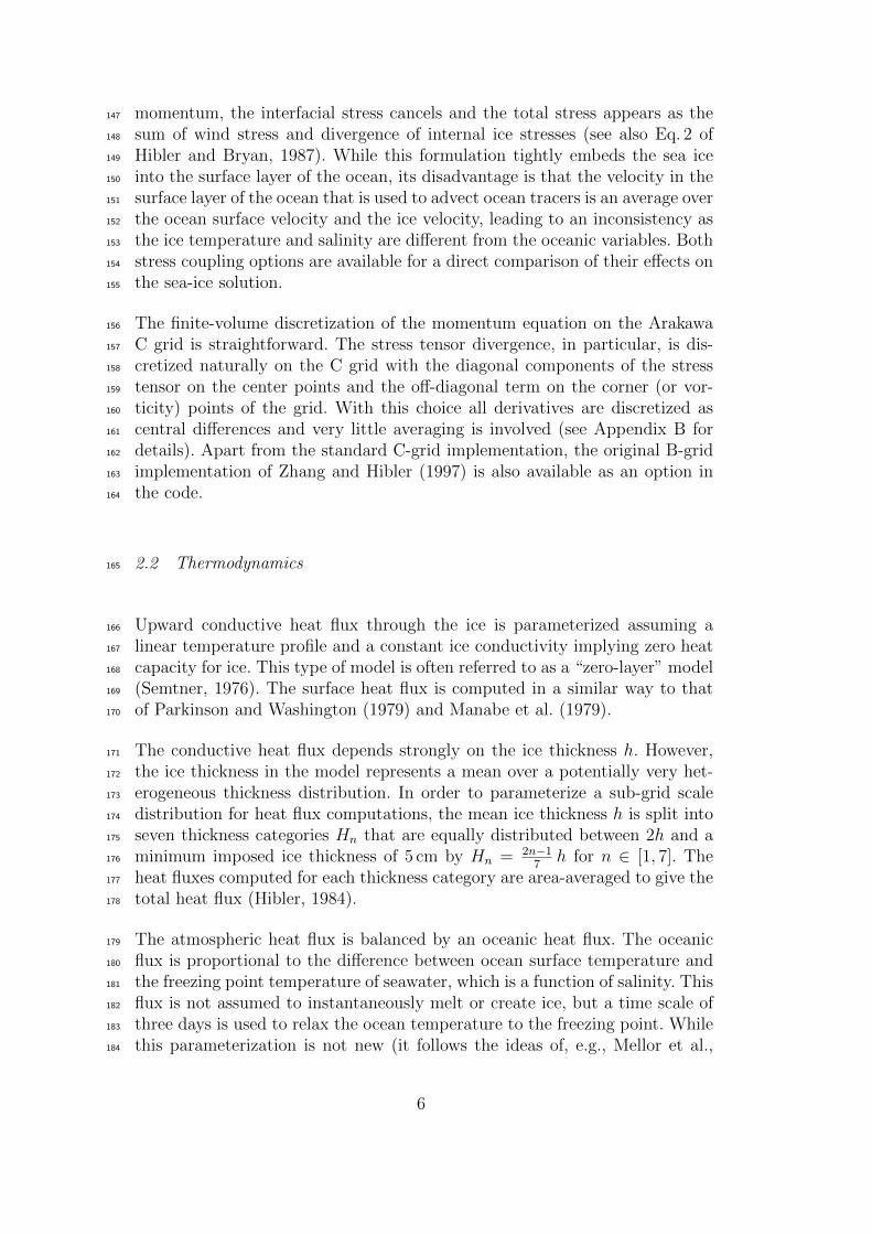
shows representative sea ice results from this simulation.238

The simulation is integrated on a cubed-sphere grid, permitting relatively even239

grid spacing throughout the domain and avoiding polar singularities (Adcroft240

et al., 2004). Each face of the cube comprises 510 by 510 grid cells for a mean241

horizontal grid spacing of 18 km. There are 50 vertical levels ranging in thick-242

ness from 10 m near the surface to approximately 450 m at a maximum model243

depth of 6150 m. The model employs the rescaled vertical coordinate “z∗”244

(Adcroft and Campin, 2004) with partial-cell formulation of Adcroft et al.245

(1997), which permits accurate representation of the bathymetry. Bathymetry246

is from the S2004 (W. Smith, unpublished) blend of the Smith and Sandwell247

(1997) and the General Bathymetric Charts of the Oceans (GEBCO) one arc-248

minute bathymetric grid. In the ocean, the non-linear equation of state of249

Jackett and McDougall (1995) is used. Vertical mixing follows Large et al.250

(1994) but with meridionally and vertically varying background vertical diffu-251

sivity; at the surface, vertical diffusivity is 4.4× 10−6 m2 s−1 at the Equator,252

3.6 × 10−6 m2 s−1 north of 70◦ N, and 1.9 × 10−5 m2 s−1 south of 30◦ S and253

between 30◦ N and 60◦ N, with sinusoidally varying values in between these254

latitudes; vertically, diffusivity increases to 1.1 × 10−4 m2 s−1 at a depth of255

6150 m as per Bryan and Lewis (1979). A 7th-order monotonicity-preserving256

advection scheme (Daru and Tenaud, 2004) is employed and there is no explicit257

horizontal diffusivity. Horizontal viscosity follows Leith (1996) but is modified258

to sense the divergent flow (Fox-Kemper and Menemenlis, 2008). The global259

ocean model is coupled to a sea ice model in a configuration similar to the case260

C-LSR-ns (see Table 1 in Section 4). The values of open water, dry ice, wet261

ice, dry snow, and wet snow albedos are, respectively, 0.15, 0.88, 0.79, 0.97,262

and 0.83. These values are relatively high compared to observations and they263

were chosen to compensate for deficiencies in the surface boundary conditions264

and to produce realistic sea ice extent (Figure 1).265

8

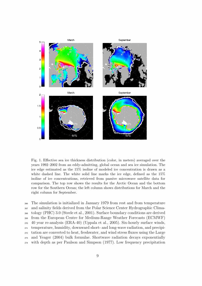
Fig. 1. Effective sea ice thickness distribution (color, in meters) averaged over theyears 1992–2002 from an eddy-admitting, global ocean and sea ice simulation. Theice edge estimated as the 15% isoline of modeled ice concentration is drawn as awhite dashed line. The white solid line marks the ice edge, defined as the 15%isoline of ice concentrations, retrieved from passive microwave satellite data forcomparison. The top row shows the results for the Arctic Ocean and the bottomrow for the Southern Ocean; the left column shows distributions for March and theright column for September.

The simulation is initialized in January 1979 from rest and from temperature266

and salinity fields derived from the Polar Science Center Hydrographic Clima-267

tology (PHC) 3.0 (Steele et al., 2001). Surface boundary conditions are derived268

from the European Centre for Medium-Range Weather Forecasts (ECMWF)269

40 year re-analysis (ERA-40) (Uppala et al., 2005). Six-hourly surface winds,270

temperature, humidity, downward short- and long-wave radiation, and precipi-271

tation are converted to heat, freshwater, and wind stress fluxes using the Large272

and Yeager (2004) bulk formulae. Shortwave radiation decays exponentially273

with depth as per Paulson and Simpson (1977). Low frequency precipitation274

9

has been adjusted using the pentad (5-day) data from the Global Precipita-275

tion Climatology Project (GPCP, Huffman et al., 2001). The time-mean river276

run-off from Large and Nurser (2001) is applied globally, except in the Arc-277

tic Ocean where monthly mean river runoff based on the Arctic Runoff Data278

Base (ARDB) and prepared by P. Winsor (personal communication, 2007) is279

specified.280

The remainder of this article discusses results from forward sensitivity exper-281

iments in a regional Arctic Ocean model, which operates on a sub-domain of,282

and which obtains open boundary conditions from, the cube76 simulation just283

described.284

4 Arctic Ocean Sensitivity Experiments285

This section presents results from regional coupled ocean and sea ice simu-286

lations of the Arctic Ocean that exercise various capabilities of the MITgcm287

sea ice model. The objective is to compare the old B-grid LSOR dynamic288

solver with the new C-grid LSOR and EVP solvers. Additional experiments289

are carried out to illustrate the differences between different lateral boundary290

conditions, ice advection schemes, ocean-ice stress formulations, and alternate291

sea ice thermodynamics.292

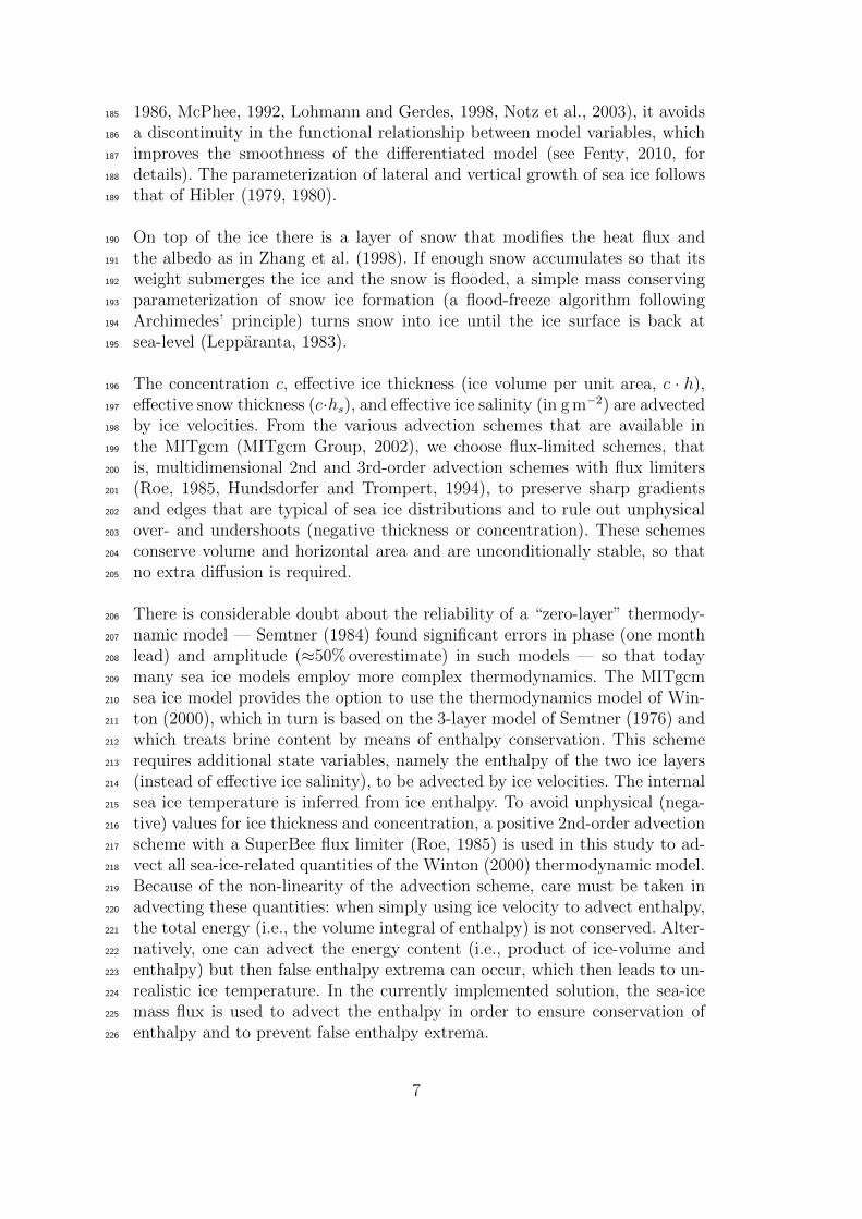
The Arctic Ocean domain has 420 by 384 grid boxes and is illustrated in Fig-293

ure 2. For each sensitivity experiment, the model is integrated from January 1,294

1992 to March 31, 2000. This time period is arbitrary and for comparison pur-295

poses only: it was chosen to be long enough to observe systematic differences296

due to details of the model configuration and short enough to allow many297

sensitivity experiments.298

Table 1 gives an overview of all the experiments discussed in this section. In299

all experiments except for DST3FL ice is advected with the original second300

order central differences scheme that requires small extra diffusion for stability301

reasons. The differences between integrations B-LSR-ns and C-LSR-ns can be302

interpreted as being caused by model finite dimensional numerical truncation.303

Both the LSOR and the EVP solvers aim to solve for the same viscous-plastic304

rheology; while the LSOR solver is an iterative scheme with a convergence305

criterion the EVP solution relaxes towards the VP solution in the limit of306

infinite intergration time. The differences between integrations C-LSR-ns, C-307

EVP-10, and C-EVP-03 are caused by fundamentally different approaches to308

regularize large bulk and shear viscosities; LSOR and other iterative tech-309

niques need to clip large viscosities, while EVP introduces elastic waves that310

damp out within one sub-cycling sequence. Both LSOR and EVP solutions311

10

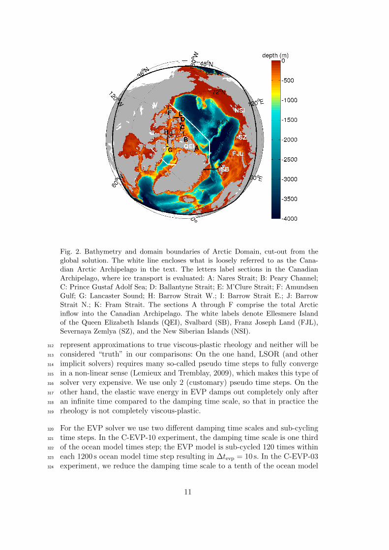
Fig. 2. Bathymetry and domain boundaries of Arctic Domain, cut-out from theglobal solution. The white line encloses what is loosely referred to as the Cana-dian Arctic Archipelago in the text. The letters label sections in the CanadianArchipelago, where ice transport is evaluated: A: Nares Strait; B: Peary Channel;C: Prince Gustaf Adolf Sea; D: Ballantyne Strait; E: M’Clure Strait; F: AmundsenGulf; G: Lancaster Sound; H: Barrow Strait W.; I: Barrow Strait E.; J: BarrowStrait N.; K: Fram Strait. The sections A through F comprise the total Arcticinflow into the Canadian Archipelago. The white labels denote Ellesmere Islandof the Queen Elizabeth Islands (QEI), Svalbard (SB), Franz Joseph Land (FJL),Severnaya Zemlya (SZ), and the New Siberian Islands (NSI).

represent approximations to true viscous-plastic rheology and neither will be312

considered “truth” in our comparisons: On the one hand, LSOR (and other313

implicit solvers) requires many so-called pseudo time steps to fully converge314

in a non-linear sense (Lemieux and Tremblay, 2009), which makes this type of315

solver very expensive. We use only 2 (customary) pseudo time steps. On the316

other hand, the elastic wave energy in EVP damps out completely only after317

an infinite time compared to the damping time scale, so that in practice the318

rheology is not completely viscous-plastic.319

For the EVP solver we use two different damping time scales and sub-cycling320

time steps. In the C-EVP-10 experiment, the damping time scale is one third321

of the ocean model times step; the EVP model is sub-cycled 120 times within322

each 1200 s ocean model time step resulting in ∆tevp = 10 s. In the C-EVP-03323

experiment, we reduce the damping time scale to a tenth of the ocean model324

11

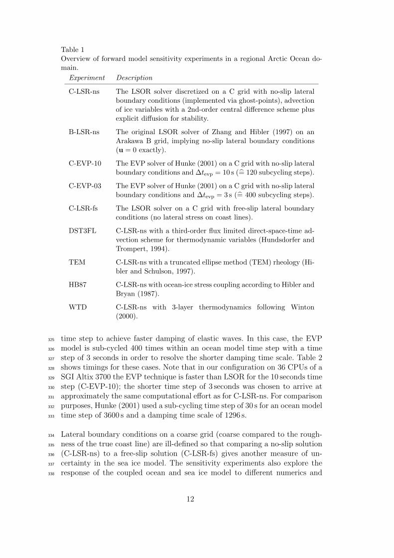
Table 1Overview of forward model sensitivity experiments in a regional Arctic Ocean do-main.

Experiment Description

C-LSR-ns The LSOR solver discretized on a C grid with no-slip lateralboundary conditions (implemented via ghost-points), advectionof ice variables with a 2nd-order central difference scheme plusexplicit diffusion for stability.

B-LSR-ns The original LSOR solver of Zhang and Hibler (1997) on anArakawa B grid, implying no-slip lateral boundary conditions(u = 0 exactly).

C-EVP-10 The EVP solver of Hunke (2001) on a C grid with no-slip lateralboundary conditions and ∆tevp = 10 s (= 120 subcycling steps).

C-EVP-03 The EVP solver of Hunke (2001) on a C grid with no-slip lateralboundary conditions and ∆tevp = 3 s (= 400 subcycling steps).

C-LSR-fs The LSOR solver on a C grid with free-slip lateral boundaryconditions (no lateral stress on coast lines).

DST3FL C-LSR-ns with a third-order flux limited direct-space-time ad-vection scheme for thermodynamic variables (Hundsdorfer andTrompert, 1994).

TEM C-LSR-ns with a truncated ellipse method (TEM) rheology (Hi-bler and Schulson, 1997).

HB87 C-LSR-ns with ocean-ice stress coupling according to Hibler andBryan (1987).

WTD C-LSR-ns with 3-layer thermodynamics following Winton(2000).

time step to achieve faster damping of elastic waves. In this case, the EVP325

model is sub-cycled 400 times within an ocean model time step with a time326

step of 3 seconds in order to resolve the shorter damping time scale. Table 2327

shows timings for these cases. Note that in our configuration on 36 CPUs of a328

SGI Altix 3700 the EVP technique is faster than LSOR for the 10 seconds time329

step (C-EVP-10); the shorter time step of 3 seconds was chosen to arrive at330

approximately the same computational effort as for C-LSR-ns. For comparison331

purposes, Hunke (2001) used a sub-cycling time step of 30 s for an ocean model332

time step of 3600 s and a damping time scale of 1296 s.333

Lateral boundary conditions on a coarse grid (coarse compared to the rough-334

ness of the true coast line) are ill-defined so that comparing a no-slip solution335

(C-LSR-ns) to a free-slip solution (C-LSR-fs) gives another measure of un-336

certainty in the sea ice model. The sensitivity experiments also explore the337

response of the coupled ocean and sea ice model to different numerics and338

12

Table 2Integration throughput on 36 CPUs of a SGI Altix 3700.

Wall clock per integration month (2232 time steps)

Experiment ice dynamics entire model

C-LSR-ns 600 sec 2887 sec

C-EVP-10 262 sec 2541 sec

C-EVP-03 875 sec 3159 sec

physics, that is, to changes in advection and diffusion properties (DST3FL), in339

rheology (TEM), in stress coupling (HB87), and in thermodynamics (WTD).340

Comparing the solutions obtained with different realizations of the model dy-341

namics is difficult because of the non-linear feedback of the ice dynamics and342

thermodynamics. Already after a few months the model trajectories have di-343

verged far enough so that velocity differences are easier to interpret within the344

first 3 months of the integration while the ice distributions are still compara-345

ble. The effect on ice-thickness of different numerics tends to accumulate along346

the time integration, resulting in larger differences - also easier to interpret -347

at the end of the integration. We choose C-LSR-ns as the reference run for all348

comparisons bearing in mind that any other choice is equally valid.349

Tables 3 and 4 summarize the differences in drift speed and effective ice thick-350

ness for all experiments. These differences are discussed in detail below.351

4.1 Ice velocities in JFM 1992352

Figure 3 shows ice velocities averaged over January, February, and March353

(JFM) of 1992 for the C-LSR-ns solution; also shown are the differences be-354

tween this reference solution and various sensitivity experiments. The velocity355

field of the C-LSR-ns solution (Figure 3a) roughly resembles the drift veloc-356

ities of some of the AOMIP (Arctic Ocean Model Intercomparison Project)357

models in a cyclonic circulation regime (Martin and Gerdes, 2007, their Fig-358

ure 6) with a Beaufort Gyre and a Transpolar Drift shifted eastwards towards359

Alaska.360

The difference between experiments C-LSR-ns and B-LSR-ns (Figure 3b) is361

most pronounced (∼ 2 cm/s) along the coastlines, where the discretization362

differs most between B and C grids. On a B grid the tangential velocity lies363

on the boundary, and is thus zero through the no-slip boundary conditions,364

whereas on the C grid it is half a cell width away from the boundary, thus365

allowing more flow. The B-LSR-ns solution has less ice drift through the Fram366

Strait and along Greenland’s East Coast; also, the flow through Baffin Bay and367

13

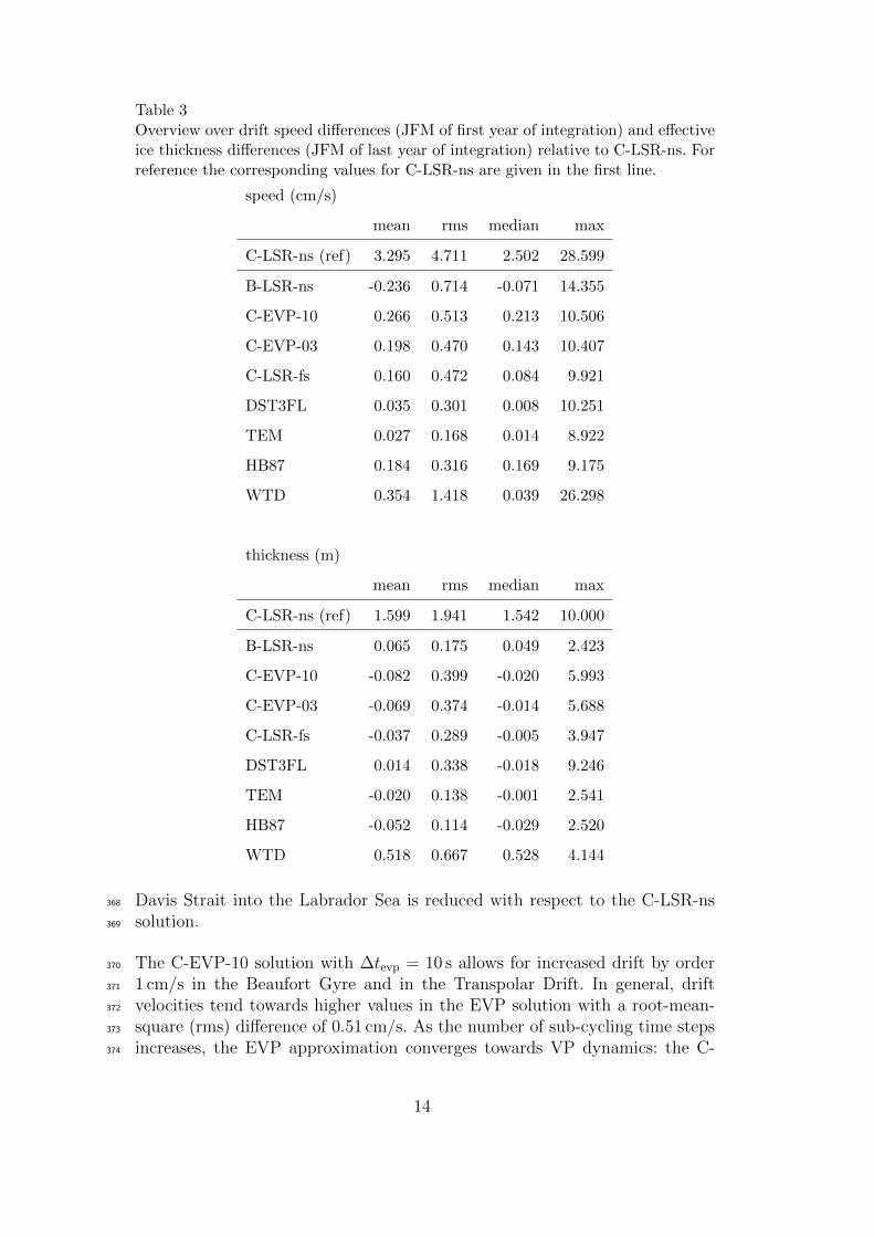
Table 3Overview over drift speed differences (JFM of first year of integration) and effectiveice thickness differences (JFM of last year of integration) relative to C-LSR-ns. Forreference the corresponding values for C-LSR-ns are given in the first line.

speed (cm/s)

mean rms median max

C-LSR-ns (ref) 3.295 4.711 2.502 28.599

B-LSR-ns -0.236 0.714 -0.071 14.355

C-EVP-10 0.266 0.513 0.213 10.506

C-EVP-03 0.198 0.470 0.143 10.407

C-LSR-fs 0.160 0.472 0.084 9.921

DST3FL 0.035 0.301 0.008 10.251

TEM 0.027 0.168 0.014 8.922

HB87 0.184 0.316 0.169 9.175

WTD 0.354 1.418 0.039 26.298

thickness (m)

mean rms median max

C-LSR-ns (ref) 1.599 1.941 1.542 10.000

B-LSR-ns 0.065 0.175 0.049 2.423

C-EVP-10 -0.082 0.399 -0.020 5.993

C-EVP-03 -0.069 0.374 -0.014 5.688

C-LSR-fs -0.037 0.289 -0.005 3.947

DST3FL 0.014 0.338 -0.018 9.246

TEM -0.020 0.138 -0.001 2.541

HB87 -0.052 0.114 -0.029 2.520

WTD 0.518 0.667 0.528 4.144

Davis Strait into the Labrador Sea is reduced with respect to the C-LSR-ns368

solution.369

The C-EVP-10 solution with ∆tevp = 10 s allows for increased drift by order370

1 cm/s in the Beaufort Gyre and in the Transpolar Drift. In general, drift371

velocities tend towards higher values in the EVP solution with a root-mean-372

square (rms) difference of 0.51 cm/s. As the number of sub-cycling time steps373

increases, the EVP approximation converges towards VP dynamics: the C-374

14

Table 4Root-mean-square differences for drift speed (JFM of first year of integration)and effective thickness (JFM of last year of integration) for the “Candian ArcticArchipelago” defined in Figure 2 and the remaining domain (“rest”). For referencethe corresponding values for C-LSR-ns are given in the first line.

rms(speed) (cm/s) rms(thickness) (m)

total CAA rest total CAA rest

C-LSR-ns (ref) 4.711 1.425 5.037 1.941 3.304 1.625

B-LSR-ns 0.714 0.445 0.747 0.175 0.369 0.117

C-EVP-10 0.513 0.259 0.543 0.399 1.044 0.105

C-EVP-03 0.470 0.234 0.497 0.374 0.982 0.095

C-LSR-fs 0.472 0.266 0.497 0.289 0.741 0.099

DST3FL 0.301 0.063 0.323 0.338 0.763 0.201

TEM 0.168 0.066 0.179 0.138 0.359 0.040

HB87 0.316 0.114 0.337 0.114 0.236 0.079

WTD 1.418 1.496 1.406 0.667 1.110 0.566

EVP-03 solution with ∆tevp = 3 s (Figure 3d) is closer to the C-LSR-ns so-375

lution (root-mean-square of 0.47 cm/s and only 0.23 cm/s in the CAA). Both376

EVP solutions have a stronger Beaufort Gyre as in Hunke and Zhang (1999).377

As expected the differences between C-LSR-fs and C-LSR-ns (Figure 3e) are378

also largest (∼ 2 cm/s) along the coastlines. The free-slip boundary condition379

of C-LSR-fs allows the flow to be faster, for example, along the East Coast of380

Greenland, the North Coast of Alaska, and the East Coast of Baffin Island, so381

that the ice drift for C-LSR-fs is on average faster than for C-LSR-ns where382

for B-LSR-ns it is on average slower.383

The more sophisticated advection scheme of DST3FL (Figure 3f) has the384

largest effect along the ice edge (see also Merryfield and Holloway, 2003),385

where the gradients of thickness and concentration are largest and differences386

in velocity can reach 5 cm/s (maximum differences are 10 cm/s at individual387

grid points). Everywhere else the effect is very small (rms of 0.3 cm/s) and388

can mostly be attributed to smaller numerical diffusion (and to the absence389

of explicit diffusion that is required for numerical stability in a simple second390

order central differences scheme). Note, that the advection scheme has an391

indirect effect on the ice drift, but a direct effect on the ice transport, and392

hence the ice thickness distribution and ice strength; a modified ice strength393

then leads to a modified drift field.394

Compared to the other parameters, the ice rheology TEM (Figure 3g) also has395

15

(a) C-LSR-ns (b) B-LSR-ns − C-LSR-ns

(c) C-EVP-10 − C-LSR-ns (d) C-EVP-03 − C-LSR-ns

Fig. 3. (a) Ice drift velocity of the C-LSR-ns solution averaged over the first 3 monthsof integration (cm/s); (b)-(h) difference between the C-LSR-ns reference solutionand solutions with, respectively, the B-grid solver, the EVP-solver with ∆tevp = 10 s,the EVP-solver with ∆tevp = 3 s, free lateral slip, a different advection scheme(DST3FL) for thermodynamic variables, the truncated ellipse method (TEM), anda different ice-ocean stress formulation (HB87). Color indicates speed or differencesof speed and vectors indicate direction only. The direction vectors represent blockaverages over eight by eight grid points at every eighth velocity point. Note thatcolor scale varies from panel to panel.

a very small (mostly < 0.5 cm/s and the smallest rms-difference of all solu-396

tions) effect on the solution. In general the ice drift tends to increase because397

there is no tensile stress and ice can drift apart at no cost. Consequently,398

the largest effect on drift velocity can be observed near the ice edge in the399

Labrador Sea. Note in experiments DST3FL and TEM the drift pattern is400

slightly changed as opposed to all other C-grid experiments, although this401

change is small.402

By way of contrast, the ice-ocean stress formulation of Hibler and Bryan (1987)403

results in stronger drift by up to 2 cm/s almost everywhere in the computa-404

tional domain (Figure 3h). The increase is mostly aligned with the general405

direction of the flow, implying that the Hibler and Bryan (1987) stress formu-406

lation reduces the deceleration of drift by the ocean.407

16

(e) C-LSR-fs − C-LSR-ns (f) DST3FL − C-LSR-ns

(g) TEM − C-LSR-ns (h) HB87 − C-LSR-ns

Fig. 3. Continued.

4.2 Integrated effect on ice volume during JFM 2000408

Figure 4a shows the effective thickness (volume per unit area) of the C-LSR-ns409

solution, averaged over January, February, and March of year 2000, that is,410

eight years after the start of the simulation. By this time of the integration,411

the differences in ice drift velocities have led to the evolution of very different412

ice thickness distributions (as shown in Figs. 4b–h) and concentrations (not413

shown) for each sensitivity experiment. The mean ice volume for the January–414

March 2000 period is also reported in Table 5.415

The generally weaker ice drift velocities in the B-LSR-ns solution, when com-416

pared to the C-LSR-ns solution, in particular through the narrow passages in417

the Canadian Arctic Archipelago, where the B-LSR-ns solution tends to block418

channels more often than the C-LSR-ns solution, lead to a larger build-up of419

ice (2 m or more) north of Greenland and north of the Archipelago in the B-420

grid solution (Figure 4b). The ice volume, however, is not larger everywhere.421

Further west there are patches of smaller ice volume in the B-grid solution,422

most likely because the Beaufort Gyre is weaker and hence not as effective in423

transporting ice westwards. There is no obvious explanation, why the ice is424

17

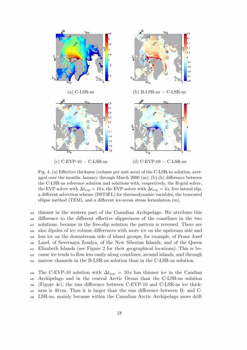
(a) C-LSR-ns (b) B-LSR-ns − C-LSR-ns

(c) C-EVP-10 − C-LSR-ns (d) C-EVP-03 − C-LSR-ns

Fig. 4. (a) Effective thickness (volume per unit area) of the C-LSR-ns solution, aver-aged over the months January through March 2000 (m); (b)-(h) difference betweenthe C-LSR-ns reference solution and solutions with, respectively, the B-grid solver,the EVP-solver with ∆tevp = 10 s, the EVP-solver with ∆tevp = 3 s, free lateral slip,a different advection scheme (DST3FL) for thermodynamic variables, the truncatedellipse method (TEM), and a different ice-ocean stress formulation (m).

thinner in the western part of the Canadian Archipelago. We attribute this425

difference to the different effective slipperiness of the coastlines in the two426

solutions, because in the free-slip solution the pattern is reversed. There are427

also dipoles of ice volume differences with more ice on the upstream side and428

less ice on the downstream side of island groups, for example, of Franz Josef429

Land, of Severnaya Zemlya, of the New Siberian Islands, and of the Queen430

Elizabeth Islands (see Figure 2 for their geographical locations). This is be-431

cause ice tends to flow less easily along coastlines, around islands, and through432

narrow channels in the B-LSR-ns solution than in the C-LSR-ns solution.433

The C-EVP-10 solution with ∆tevp = 10 s has thinner ice in the Candian434

Archipelago and in the central Arctic Ocean than the C-LSR-ns solution435

(Figure 4c); the rms difference between C-EVP-10 and C-LSR-ns ice thick-436

ness is 40 cm. Thus it is larger than the rms difference between B- and C-437

LSR-ns, mainly because within the Canadian Arctic Archipelago more drift438

18

(e) C-LSR-fs − C-LSR-ns (f) DST3FL − C-LSR-ns

(g) TEM − C-LSR-ns (h) HB87 − C-LSR-ns

Fig. 4. Continued.

Table 5Arctic ice volume averaged over Jan–Mar 2000, in km3. Mean ice transport (andstandard deviation in parenthesis) for the period Jan 1992 – Dec 1999 through theFram Strait (FS), the total northern inflow into the Canadian Arctic Archipelago(CAA), and the export through Lancaster Sound (LS), in km3 y−1.

Volume Sea ice transport (km3 yr−1)

Experiment (km3) FS CAA LS

C-LSR-ns 24,769 2196 (1253) 70 (224) 77 (110)

B-LSR-ns 23,824 2126 (1278) 34 (122) 43 (76)

C-EVP-10 22,633 2174 (1260) 186 (496) 133 (128)

C-EVP-03 22,819 2161 (1252) 175 (461) 123 (121)

C-LSR-fs 23,286 2236 (1289) 80 (276) 91 (85)

DST3FL 24,023 2191 (1261) 88 (251) 84 (129)

TEM 23,529 2222 (1258) 60 (242) 87 (112)

HB87 23,060 2256 (1327) 64 (230) 77 (114)

WTD 31,634 2761 (1563) 23 (140) 94 (63)

19

in C-EVP-10 leads to faster ice export and to reduced effective ice thickness.439

With a shorter time step (∆tevp = 3 s) the EVP solution converges towards440

the LSOR solution in the central Arctic (Figure 4d). In the narrow straits in441

the Archipelago, however, the ice thickness is not affected by the shorter time442

step and the ice is still thinner by 2 m or more, as it is in the EVP solution443

with ∆tevp = 10 s.444

Imposing a free-slip boundary condition in C-LSR-fs leads to much smaller445

differences to C-LSR-ns (Figure 4e) than the transition from the B grid to the446

C grid, except in the Canadian Arctic Archipelago, where the free-slip solution447

allows more flow (see Table 4). There, it reduces the effective ice thickness by448

2 m or more where the ice is thick and the straits are narrow (leading to an449

overall larger rms-difference than the B-LSR-ns solution, see Table 4). Dipoles450

of ice thickness differences can also be observed around islands because the451

free-slip solution allows more flow around islands than the no-slip solution.452

The differences in the Central Arctic are much smaller in absolute value than453

the differences in the Canadian Arctic Archipelago although there are also454

interesting changes in the ice-distribution in the interior: Less ice in the Central455

Arctic is most likely caused by more export (see Table 5).456

The remaining sensitivity experiments, DST3FL, TEM, and HB87, have the457

largest differences in effective ice thickness along the north coasts of Greenland458

and Ellesmere Island in the Canadian Arctic Archipelago. Although using the459

TEM rheology and the Hibler and Bryan (1987) ice-ocean stress formulation460

has different effects on the initial ice velocities (Figure 3g and h), both experi-461

ments have similarly reduced ice thicknesses in this area. The 3rd-order advec-462

tion scheme (DST3FL) has an opposite effect of similar magnitude, pointing463

towards more implicit lateral stress with this numerical scheme. The HB87 ex-464

periment shows ice thickness reduction in the entire Arctic basin greater than465

in any other experiment, possibly because more drift leads to faster export of466

ice.467

Figure 5 summarizes Figures 3 and 4 by showing histograms of sea ice thickness468

and drift velocity differences to the reference C-LSR-ns. The black line is the469

cumulative number grid points in percent of all grid points of all models where470

differences up to the value on the abscissa are found. For example, ice thickness471

differences up to 50 cm are found in 90% of all grid points, or equally differences472

above 50 cm are only found in 10% of all grid points. The colors indicate the473

distribution of these grid points between the various experiments. For example,474

65% to 90% of grid points with ice thickness differences between 40 cm and475

1 m are found in the run WTD. The runs B-LSR-ns, C-EVP-10, and HB87476

only have a fairly large number of grid points with differences below 40 cm.477

B-LSR-ns and WTD dominate nearly all velocity differences. The remaining478

contributions are small except for small differences below 1 cm/s. Only very479

few points contribute to very large differences in thickness (above 1 m) and480

20

Fig. 5. Histograms of ice thickness and drift velocity differences relative to C-LSR-ns;the bin-width is 2 cm for thickness and 0.1 cm/s for speed. The black line is thecumulative number of grid points in percent of all grid points. The colors indicatethe distribution of these grid points between the various experiments in percent ofthe black line.

velocity (above 4 cm/s) indicated by the small slope of the cumlative number481

of grid point (black line).482

4.3 Ice transports483

The difference in ice volume and in ice drift velocity between the various484

sensitivity experiments has consequences for sea ice export from the Arctic485

Ocean. As an illustration (other years are similar), Figure 6 shows the 1996486

time series of sea ice transports through the northern edge of the Canadian487

Arctic Archipelago, through Lancaster Sound, and through Fram Strait for488

each model sensitivity experiment. The mean and standard deviation of these489

ice transports, over the period January 1992 to December 1999, are reported490

in Table 5. In addition to sea ice dynamics, there are many factors, e.g., atmo-491

spheric and oceanic forcing, drag coefficients, and ice strength, that control sea492

ice export. Although calibrating these various factors is beyond the scope of493

this manuscript, it is nevertheless instructive to compare the values in Table 5494

with published estimates, as is done next. This is a necessary step towards con-495

21

Fig. 6. Transports of sea ice during 1996 for model sensitivity experiments listed inTable 1. Top panel shows flow through the northern edge of the Canadian ArcticArchipelago (Sections A–F in Figure 2), middle panel shows flow through LancasterSound (Section G), and bottom panel shows flow through Fram Strait (Section K).Positive values indicate sea ice flux out of the Arctic Ocean. The time series aresmoothed using a monthly running mean. The mean range, i.e., the time-meandifference between the model solution with maximum flux and that with minimumflux, is computed over the period January 1992 to December 1999.

straining this model with data, a key motivation for developing the MITgcm496

sea ice model and its adjoint.497

The export through Fram Strait for all the sensitivity experiments is consistent498

with the value of 2300 ± 610 km3 yr−1 reported by Serreze et al. (2006, and499

references therein). Although Arctic sea ice is exported to the Atlantic Ocean500

principally through the Fram Strait, Serreze et al. (2006) estimate that a501

22

considerable amount of sea ice (∼ 160 km3 yr−1) is also exported through the502

Canadian Arctic Archipelago. This estimate, however, is associated with large503

uncertainties. For example, Dey (1981) estimates an inflow into Baffin Bay of504

370 to 537 km3 yr−1 but a flow of only 102 to 137 km3 yr−1 further upstream in505

Barrow Strait in the 1970’s from satellite images; Aagaard and Carmack (1989)506

give approximately 155 km3 yr−1 for the export through the CAA. The recent507

estimates of Agnew et al. (2008) for Lancaster Sound are lower: 102 km3 yr−1.508

The model results suggest annually averaged ice transports through Lancaster509

Sound ranging from 43 to 133 km3 yr−1 and total northern inflow of 34 to510

186 km3 yr−1 (Table 5). These model estimates and their standard deviations511

cannot be rejected based on the observational estimates.512

Generally, the EVP solutions have the highest maximum (export out of the513

Arctic) and lowest minimum (import into the Arctic) fluxes as the drift veloc-514

ities are largest in these solutions. In the extreme of the Nares Strait, which515

is only a few grid points wide in our configuration, both B- and C-grid LSOR516

solvers lead to practically no ice transport, while the EVP solutions allow517

200–500 km3 yr−1 in summer (not shown). Tang et al. (2004) report 300 to518

350 km3 yr−1 and Kwok (2005) 130± 65 km3 yr−1. As as consequence, the im-519

port into the Canadian Arctic Archipelago is larger in all EVP solutions than520

in the LSOR solutions. The B-LSR-ns solution is even smaller by another521

factor of two than the C-LSR solutions.522

4.4 Thermodynamics523

The last sensitivity experiment (WTD) listed in Table 1 is carried out using524

the 3-layer thermodynamics model of Winton (2000). This experiment has525

different albedo and basal heat exchange formulations from all the other ex-526

periments. Although, the upper-bound albedo values for dry ice, dry snow, and527

wet snow are the same as for the zero-layer model, the ice albedos in WTD are528

computed following Hansen et al. (1983) and can become much smaller as a529

function of thickness h, with a minimum value of 0.2 exp(−h/0.44 m). Further530

the snow age is taken into account when computing the snow albedo. With531

the same values for wet snow (0.83), dry snow (0.97), and dry ice (0.88) as532

for the zero-heat-capacity model (see Section 3), this results in albedos that533

range from 0.22 to 0.95 (not shown). Similarly, large differences can be found534

in the basal heat exchange parameterizations. For this reason, the resulting535

ice velocities, volume, and transports have not been included in the earlier536

comparisons. However, this experiment gives another measure of uncertainty537

associated with ice modeling. The key difference with the “zero-layer” thermo-538

dynamic model is a delay in the seaice cycle of approximately one month in the539

maximum sea-ice thickness and two months in the minimum sea-ice thickness.540

This is shown in Figure 7, which compares the mean sea-ice thickness seasonal541

23

Fig. 7. Seasonal cycle of mean sea-ice thickness (cm) in a sector in the western Arctic(75◦ N to 85◦ N and 180◦ W to 140◦ W) averaged over 1992–2000 of experimentsC-LSR-ns and WTD.

cycle of experiments with the zero-heat-capacity (C-LSR-ns) and three-layer542

(WTD) thermodynamic model. The mean ice thickness is computed for a sec-543

tor in the western Arctic (75◦ N to 85◦ N and 180◦ W to 140◦ W) in order to544

avoid confounding thickness and extent differences. Similar to Semtner (1976),545

the seasonal cycle for the “zero-layer” model (gray dashed line) is almost twice546

as large as for the three-layer thermodynamic model.547

5 Conclusions548

We have shown that changes in discretization details, in boundary conditions,549

and in sea-ice-dynamics formulation lead to considerable differences in model550

results. Notably the sea-ice-dynamics formulation, e.g., B-grid versus C-grid or551

EVP versus LSOR, has as much or even greater influence on the solution than552

physical parameterizations, e.g., free-slip versus no-slip boundary conditions.553

This is especially true554

• in regions of convergence (see ice thickness north of Greenland in Fig. 4),555

• along coasts (see eastern coast of Greenland in Fig. 3 where velocity differ-556

24

ences are apparent),557

• and in the vicinity of straits (see the Canadian Arctic Archipelago in Figs. 3558

and 4).559

These experiments demonstrate that sea-ice export from the Arctic into both560

the Baffin Bay and the GIN (Greenland/Iceland/Norwegian) Sea regions is561

highly sensitive to numerical formulation. Changes in export in turn impact562

deep-water mass formation in the northern North Atlantic. Therefore uncer-563

tainties due to numerical formulation might potentially have wide reaching564

impacts outside of the Arctic.565

The relatively large differences between solutions with different dynamical566

solvers is somewhat surprising. The expectation was that the solution tech-567

nique should not affect the solution to a higher degree than actually modifying568

the equations. The EVP solutions tend to produce effectively “weaker” ice that569

yields more easily to stress than the LSOR solutions, similar to the findings570

in Hunke and Zhang (1999). The differences between LSOR and EVP can, in571

part, stem from incomplete convergence of the solvers due to linearization and572

due to different methods of linearization (Hunke, 2001, and B. Tremblay, pers.573

comm. 2008). We note that the EVP-to-LSOR differences decrease with de-574

creasing sub-cycling time step but that the difference remains significant even575

at a 3-second sub-cycling period. For the LSOR solutions we use 2 pseudo576

time steps so that the convergence of the non-linear momentum equations577

may not be complete. This effect is most likely reduced and constrained to578

small areas as in Lemieux and Tremblay (2009) because of the small time step579

that we used. Whether more pseudo time steps make the LSOR solution gen-580

erate weaker ice requires further investigation. Preliminary tests indicate that581

the viscosity increases with increasing number of LSOR pseudo time steps,582

especially in areas of thick ice (not shown).583

Other numerical formulation choices that were tested include switching from584

one horizontal grid staggering (C-grid) to another (B-grid). This change signif-585

icantly affects narrow straits, for example, in the Canadian Arctic Archipelago,586

and subsequent conditions upstream and downstream of the straits. It also587

affects flows of ice along the West Greenland coast. Similar, but smaller, dif-588

ferences between B-grid and C-grid sea ice solutions were noted in the coarser-589

resolution study of Bouillon et al. (2009). The differences between the no-slip590

and free-slip lateral boundary conditions are also most significant near the591

coast. As in the case of oceanic boundary conditions (Adcroft and Marshall,592

1998), we expect that the changes are due to the effective “slipperiness” of593

the coastline boundary condition.594

The flux-limited scheme without explicit diffusion (DST3FL) is recommended.595

This is because the flux-limited scheme preserves sharp gradients and edges596

that are typical of sea ice distributions and because it avoids unphysical (neg-597

25

ative) values for ice thickness and concentration (see also Merryfield and Hol-598

loway, 2003). The flux limited scheme conserves volume and horizontal area599

and is unconditionally stable, so that no extra diffusion is required.600

Changing the ice rheology to the truncated ellipse method (TEM) primar-601

ily impacts the solution in the Canadian Arctic Archipelago and the West602

Greenland coast as does altering the stress formulation on the ice solution.603

We interpret this result as indicating that the CAA and West Greenland cur-604

rent are regions of high-sensitivity. Here, more ice leads to a rigid structure605

that inhibits ice flow and yields ice accumulation upstream.606

Although the Hibler and Bryan (1987) stress formulation appears more natural607

for advecting sea ice, the advection of oceanic properties is problematic: Ther-608

modynamic and passive tracers in the top ocean model level are advected with609

a velocity that is the average over ice drift and ocean currents rather than an610

average of surface oceanic currents alone. For our purposes, the preferred ice-611

ocean coupling uses the rescaled vertical coordinates of Campin et al. (2008),612

which allows the ice to depress the ocean surface according to its thickness613

and buoyancy.614

A few comments regarding the robustness of our results against choice of615

forcing, integration period, and horizontal resolution follow. Strictly speaking,616

our results refer to an 8-year integration with 18 km horizontal grid spacing.617

We find that the differences between the solutions have an obvious trend after618

the first season but that this trend flattens out after a few seasons. We do619

not expect the differences to increase dramatically with additional integration620

time, since the simulated multi-year sea ice has reached a quasi equilibrium.621

Surface atmospheric conditions are specified every 6 hours. Models with weaker622

ice can react more quickly to a change in wind forcing, therefore we speculate623

that the differences between EVP and LSOR integrations would change with624

different forcing: less variable wind forcing would lead to smaller differences,625

while larger fluctuations in the forcing would increase them. In the same way,626

we expect that with coarser grids, the ocean component is much less variable627

so that in this case one will only find smaller differences between ice models.628

The MITgcm sea ice model enables, within the same code, the direct compari-629

son of various widely used dynamics and thermodynamics model components.630

What sets apart the MITgcm sea ice model from other current-generation sea631

ice models is the ability to derive an accurate, stable, and efficient adjoint632

model using automatic differentiation source transformation tools. This capa-633

bility is the topic of a companion, second paper. The adjoint model greatly634

facilitates and enhances exploration of the model’s parameter space. It lays635

the foundation for coupled ocean and sea ice state estimation.636

26

A Dynamics637

For completeness we provide more details on the ice dynamics of the sea-ice638

model. The momentum equations are639

mDu

Dt= −mfk× u + τ air + τ ocean −m∇φ(0) + F, (A.1)640

where m = mi +ms is the ice and snow mass per unit area; u = ui + vj is the641

ice velocity vector; i, j, and k are unit vectors in the x, y, and z directions,642

respectively; f is the Coriolis parameter; τ air and τ ocean are the wind-ice643

and ocean-ice stresses, respectively; g is the gravity acceleration; ∇φ(0) is the644

gradient (or tilt) of the sea surface height; φ(0) = gη+pa/ρ0 +mg/ρ0 is the sea645

surface height potential in response to ocean dynamics (gη), to atmospheric646

pressure loading (pa/ρ0, where ρ0 is a reference density) and a term due to647

snow and ice loading (Campin et al., 2008); and F = ∇·σ is the divergence of648

the internal ice stress tensor σij. Advection of sea-ice momentum is neglected.649

The wind and ice-ocean stress terms are given by650

τ air =ρairCair|Uair − u|Rair(Uair − u),651

τ ocean =ρoceanCocean|Uocean − u|Rocean(Uocean − u),652653

where Uair/ocean are the surface winds of the atmosphere and surface cur-654

rents of the ocean, respectively; Cair/ocean are air and ocean drag coefficients;655

ρair/ocean are reference densities; and Rair/ocean are rotation matrices that act656

on the wind/current vectors. In this paper both rotation angles are set to zero.657

For an isotropic system the stress tensor σij (i, j = 1, 2) can be related to the658

ice strain rate and strength by a nonlinear viscous-plastic (VP) constitutive659

law (Hibler, 1979, Zhang and Hibler, 1997):660

σij = 2η(εij, P )εij + [ζ(εij, P )− η(εij, P )] εkkδij −P

2δij. (A.2)661

The ice strain rate is given by662

εij =1

2

(∂ui∂xj

+∂uj∂xi

).663

The maximum ice pressure Pmax, a measure of ice strength, depends on both664

thickness h and compactness (concentration) c:665

Pmax = P ∗c h e[C∗·(1−c)], (A.3)666

with the constants P ∗ and C∗; we use P ∗ = 27 500 N m−2 and C∗ = 20. Thenonlinear bulk and shear viscosities η and ζ are functions of ice strain rateinvariants and ice strength such that the principal components of the stress

27

lie on an elliptical yield curve with the ratio of major to minor axis e equal to2; they are given by:

ζ = min

(Pmax

2 max(∆,∆min), ζmax

)

η =ζ

e2

with the abbreviation

∆ =[(ε211 + ε222

)(1 + e−2) + 4e−2ε212 + 2ε11ε22(1− e−2)

] 12 .

In the simulations of this paper, the bulk viscosities are bounded above by im-667

posing both a minimum ∆min = 10−11 s−1 and a maximum ζmax = Pmax/∆∗,668

where ∆∗ = (5× 1012/2× 104) s−1. For stress tensor computation the replace-669

ment pressure P = 2 ∆ζ (Hibler and Ip, 1995) is used so that the stress state670

always lies on the elliptic yield curve by definition.671

In the so-called truncated ellipse method (experiment TEM) the shear vis-672

cosity η is capped to suppress any tensile stress (Hibler and Schulson, 1997,673

Geiger et al., 1998):674

η = min

ζ

e2,

P2− ζ(ε11 + ε22)√

(ε11 + ε22)2 + 4ε212

. (A.4)675

In the current implementation, the VP-model is integrated with the semi-676

implicit line successive over relaxation (LSOR)-solver of Zhang and Hibler677

(1997), which allows for long time steps that, in our case, are limited by the678

explicit treatment of the Coriolis term. The explicit treatment of the Coriolis679

term does not represent a severe limitation because it restricts the time step680

to approximately the same length as in the ocean model where the Coriolis681

term is also treated explicitly.682

Hunke and Dukowicz (1997) introduced an elastic contribution to the strain683

rate in order to regularize Eq. A.2 in such a way that the resulting elastic-684

viscous-plastic (EVP) and VP models are identical at steady state,685

1

E

∂σij∂t

+1

2ησij +

η − ζ4ζη

σkkδij +P

4ζδij = εij. (A.5)686

The EVP-model uses an explicit time stepping scheme with a short time step.687

According to the recommendation of Hunke and Dukowicz (1997), the EVP-688

model is stepped forward in time O(120) times within the physical ocean model689

time step, to allow for elastic waves to disappear. Because the scheme does690

not require a matrix inversion it is fast in spite of the small internal time step691

28

and simple to implement on parallel computers (Hunke and Dukowicz, 1997).692

For completeness, we repeat the equations for the components of the stress693

tensor σ1 = σ11 + σ22, σ2 = σ11 − σ22, and σ12. Introducing the divergence694

DD = ε11 + ε22, and the horizontal tension and shearing strain rates, DT =695

ε11 − ε22 and DS = 2ε12, respectively, and using the above abbreviations, the696

equations A.5 can be written as:697

∂σ1

∂t+σ1

2T+

P

2T=

P

2T∆DD (A.6)698

∂σ2

∂t+σ2e

2

2T=

P

2T∆DT (A.7)699

∂σ12

∂t+σ12e

2

2T=

P

4T∆DS (A.8)700

701

Here, the elastic parameter E is redefined in terms of a damping time scale Tfor elastic waves

E =ζ

T.

T = E0∆t with the tunable parameter E0 < 1 and the external (long) time702

step ∆t. In experiment C-EVP-10 use E0 = 13

which is close to value of 0.36703

used by Hunke (2001). In experiment C-EVP-03 we use E0 = 110

resulting in704

T = 120 s for our choice of ∆t.705

B Finite-volume discretization of the stress tensor divergence706

On an Arakawa C grid, ice thickness and concentration and thus ice strength707

P and bulk and shear viscosities ζ and η are naturally defined at C-points in708

the center of the grid cell. Discretization requires only averaging of ζ and η to709

vorticity or Z-points at the bottom left corner of the cell to give ζZ

and ηZ .710

In the following, the superscripts indicate location at Z or C points, distance711

across the cell (F), along the cell edge (G), between u-points (U), v-points712

(V), and C-points (C). The control volumes of the u- and v-equations in the713

grid cell at indices (i, j) are Awi,j and Asi,j, respectively. With these definitions714

(which follow the model code documentation at http://mitgcm.org except715

that vorticity or ζ-points have been renamed to Z-points in order to avoid716

29

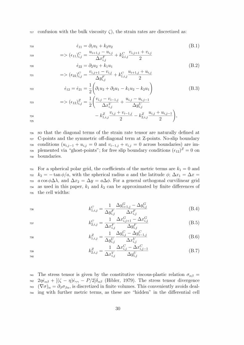
confusion with the bulk viscosity ζ), the strain rates are discretized as:717

ε11 = ∂1u1 + k2u2 (B.1)718

=> (ε11)Ci,j =ui+1,j − ui,j

∆xFi,j+ kC2,i,j

vi,j+1 + vi,j2

719

ε22 = ∂2u2 + k1u1 (B.2)720

=> (ε22)Ci,j =vi,j+1 − vi,j

∆yFi,j+ kC1,i,j

ui+1,j + ui,j2

721

ε12 = ε21 =1

2

(∂1u2 + ∂2u1 − k1u2 − k2u1

)(B.3)722

=> (ε12)Zi,j =1

2

(vi,j − vi−1,j

∆xVi,j+ui,j − ui,j−1

∆yUi,j723

− kZ1,i,jvi,j + vi−1,j

2− kZ2,i,j

ui,j + ui,j−1

2

),724

725

so that the diagonal terms of the strain rate tensor are naturally defined at726

C-points and the symmetric off-diagonal term at Z-points. No-slip boundary727

conditions (ui,j−1 + ui,j = 0 and vi−1,j + vi,j = 0 across boundaries) are im-728

plemented via “ghost-points”; for free slip boundary conditions (ε12)Z = 0 on729

boundaries.730

For a spherical polar grid, the coefficients of the metric terms are k1 = 0 and731

k2 = − tanφ/a, with the spherical radius a and the latitude φ; ∆x1 = ∆x =732

a cosφ∆λ, and ∆x2 = ∆y = a∆φ. For a general orthogonal curvilinear grid733

as used in this paper, k1 and k2 can be approximated by finite differences of734

the cell widths:735

kC1,i,j =1

∆yFi,j

∆yGi+1,j −∆yGi,j∆xFi,j

(B.4)736

kC2,i,j =1

∆xFi,j

∆xGi,j+1 −∆xGi,j∆yFi,j

(B.5)737

kZ1,i,j =1

∆yUi,j

∆yCi,j −∆yCi−1,j

∆xVi,j(B.6)738

kZ2,i,j =1

∆xVi,j

∆xCi,j −∆xCi,j−1

∆yUi,j(B.7)739

740

The stress tensor is given by the constitutive viscous-plastic relation σαβ =741

2ηεαβ + [(ζ − η)εγγ − P/2]δαβ (Hibler, 1979). The stress tensor divergence742

(∇σ)α = ∂βσβα, is discretized in finite volumes. This conveniently avoids deal-743

ing with further metric terms, as these are “hidden” in the differential cell744

30

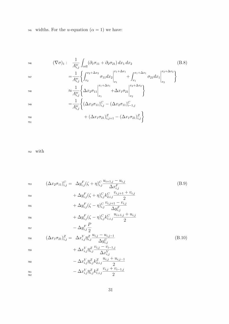
widths. For the u-equation (α = 1) we have:745

(∇σ)1 :1

Awi,j

∫cell

(∂1σ11 + ∂2σ21) dx1 dx2 (B.8)746

=1

Awi,j

{∫ x2+∆x2

x2σ11dx2

∣∣∣∣∣x1+∆x1

x1

+∫ x1+∆x1

x1σ21dx1

∣∣∣∣∣x2+∆x2

x2

}747

≈ 1

Awi,j

{∆x2σ11

∣∣∣∣∣x1+∆x1

x1

+∆x1σ21

∣∣∣∣∣x2+∆x2

x2

}748

=1

Awi,j

{(∆x2σ11)Ci,j − (∆x2σ11)Ci−1,j749

+ (∆x1σ21)Zi,j+1 − (∆x1σ21)Zi,j

}750

751

with752

(∆x2σ11)Ci,j = ∆yFi,j(ζ + η)Ci,jui+1,j − ui,j

∆xFi,j(B.9)753

+ ∆yFi,j(ζ + η)Ci,jkC2,i,j

vi,j+1 + vi,j2

754

+ ∆yFi,j(ζ − η)Ci,jvi,j+1 − vi,j

∆yFi,j755

+ ∆yFi,j(ζ − η)Ci,jkC1,i,j

ui+1,j + ui,j2

756

−∆yFi,jP

2757

(∆x1σ21)Zi,j = ∆xVi,jηZi,j

ui,j − ui,j−1

∆yUi,j(B.10)758

+ ∆xVi,jηZi,j

vi,j − vi−1,j

∆xVi,j759

−∆xVi,jηZi,jk

Z2,i,j

ui,j + ui,j−1

2760

−∆xVi,jηZi,jk

Z1,i,j

vi,j + vi−1,j

2761

762

31

Similarly, we have for the v-equation (α = 2):763

(∇σ)2 :1

Asi,j

∫cell

(∂1σ12 + ∂2σ22) dx1 dx2 (B.11)764

=1

Asi,j

{∫ x2+∆x2

x2σ12dx2

∣∣∣∣∣x1+∆x1

x1

+∫ x1+∆x1

x1σ22dx1

∣∣∣∣∣x2+∆x2

x2

}765

≈ 1

Asi,j

{∆x2σ12

∣∣∣∣∣x1+∆x1

x1

+∆x1σ22

∣∣∣∣∣x2+∆x2

x2

}766

=1

Asi,j

{(∆x2σ12)Zi+1,j − (∆x2σ12)Zi,j767

+ (∆x1σ22)Ci,j − (∆x1σ22)Ci,j−1

}768

769

with770

(∆x1σ12)Zi,j = ∆yUi,jηZi,j

ui,j − ui,j−1

∆yUi,j(B.12)771

+ ∆yUi,jηZi,j

vi,j − vi−1,j

∆xVi,j772

−∆yUi,jηZi,jk

Z2,i,j

ui,j + ui,j−1

2773

−∆yUi,jηZi,jk

Z1,i,j

vi,j + vi−1,j

2774

(∆x2σ22)Ci,j = ∆xFi,j(ζ − η)Ci,jui+1,j − ui,j

∆xFi,j(B.13)775

+ ∆xFi,j(ζ − η)Ci,jkC2,i,j

vi,j+1 + vi,j2

776

+ ∆xFi,j(ζ + η)Ci,jvi,j+1 − vi,j

∆yFi,j777

+ ∆xFi,j(ζ + η)Ci,jkC1,i,j

ui+1,j + ui,j2

778

−∆xFi,jP

2779

780

Acknowledgements781

We thank Jinlun Zhang for providing the original B-grid code and for many782

helpful discussions. ML thanks Elizabeth Hunke for multiple explanations and783

Sergey Danilov and Rudiger Gerdes for comments on the manuscript. This784

work was supported by NSF award ARC-0804150, DOE award DE-FG02-785

08ER64592, and NASA award NNG06GG98G. It is a contribution to the786

ECCO2 project sponsored by the NASA Modeling Analysis and Prediction787

32

(MAP) program and to the ECCO-GODAE project sponsored by the National788

Oceanographic Partnership Program (NOPP). Computing resources were pro-789

vided by NASA/ARC, NCAR/CSL, and JPL/SVF.790

References791

Aagaard, K., Carmack, E. C., 1989. The role of sea ice and other fresh waters792

in the Arctic circulation. J. Geophys. Res. 94 (C10), 14,485–14,498.793

Adcroft, A., Campin, J.-M., 2004. Rescaled height coordinates for accurate794

representation of free-surface flows in ocean circulation models. Ocean Mod-795

elling 7 (3-4), 269–284.796

Adcroft, A., Campin, J.-M., Hill, C. N., Marshall, J. C., 2004. Implementation797

of an atmosphere-ocean general circulation model on the expanded spherical798

cube. Mon. Weather Rev. 132 (12), 2845–2863.799

Adcroft, A., Hill, C., Marshall, J., 1997. Representation of topography by800

shaved cells in a height coordinate ocean model. Mon. Weather Rev. 125 (9),801

2293–2315.802

Adcroft, A., Marshall, D., 1998. How slippery are piecewise-constant coastlines803

in numerical ocean models? Tellus 50A, 95–108.804

Agnew, T., Lambe, A., Long, D., 2008. Estimating sea ice area flux across the805

Canadian Arctic Archipelago using enhanced AMSR-E. J. Geophys. Res.806

113, C10011.807

Bouillon, S., Maqueda, M. A. M., Legat, V., Fichefet, T., 2009. An elastic-808

viscous-plastic sea ice model formulated on Arakawa B and C grids. Ocean809

Modelling 27 (3–4), 174–184.810

Bryan, K., Lewis, L. J., 1979. A water mass model of the world ocean. J.811

Geophys. Res. 84 (C5), 2503–2517.812

Campin, J.-M., Marshall, J., Ferreira, D., 2008. Sea-ice ocean coupling using813

a rescaled vertical coordinate z∗. Ocean Modelling 24 (1–2), 1–14.814

Cavalieri, D. J., Parkinson, C., 2008. Antarctic sea ice variability and trends,815

1979–2006. J. Geophys. Res. 113, C07004.816

Daru, V., Tenaud, C., 2004. High order one-step monotonicity-preserving817

schemes for unsteady compressible flow calculations. J. Comput. Phys.818

193 (2), 563–594.819

Dey, B., 1981. Monitoring winter sea ice dynamics in the Canadian Arctic820

with NOAA-TIR images. J. Geophys. Res. 86 (C4), 3223–3235.821

Fenty, I., 2010. State estimation of the Labrador Sea with a coupled ocean/sea-822

ice adjoint model. Ph.D. thesis, MIT, Program in Atmosphere, Ocean and823

Climate (PAOC), Cambridge (MA), USA.824

Fox-Kemper, B., Menemenlis, D., 2008. Can large eddy simulation techniques825

improve mesoscale rich ocean models? In: Hecht, M., Hasumi, H. (Eds.),826

Ocean Modeling in an Eddying Regime. AGU, Washington, D.C., pp. 319–827

338.828

33

Geiger, C. A., Hibler, III, W. D., Ackley, S. F., 1998. Large-scale sea ice829

drift and deformation: Comparison between models and observations in the830

western Weddell Sea during 1992. J. Geophys. Res. 103 (C10), 21893–21913.831

Griewank, A., 2000. Evaluating Derivatives. Principles and Techniques of832

Algorithmic Differentiation. Vol. 19 of Frontiers in Applied Mathematics.833

SIAM, Philadelphia.834

Hansen, J., Russell, G., Rind, D., Stone, P., Lacis, A., Lebedeff, S., Ruedy,835

R., Travis, L., 1983. Efficient three-dimensional global models for climate836

studies: Models I and II. Mon. Weather Rev. 111, 609–662.837

Harder, M., Fischer, H., 1999. Sea ice dynamics in the Weddell Sea simulated838

with an optimzed model. J. Geophys. Res. 104 (C5), 11,151–11,162.839

Heimbach, P., January 2008. The MITgcm/ECCO adjoint modelling infras-840

tructure. CLIVAR Exchanges 44 (Volume 13, No. 1), 13–17.841

Hibler, III, W. D., 1979. A dynamic thermodynamic sea ice model. J. Phys.842

Oceanogr. 9 (4), 815–846.843

Hibler, III, W. D., 1980. Modeling a variable thickness sea ice cover. Mon.844

Weather Rev. 108 (2), 1943–1973.845

Hibler, III, W. D., 1984. The role of sea ice dynamics in modeling co2 increases.846

In: Hansen, J. E., Takahashi, T. (Eds.), Climate processes and climate sen-847

sitivity. Vol. 29 of Geophysical Monograph. AGU, Washington, D.C., pp.848

238–253.849

Hibler, III, W. D., Bryan, K., 1987. A diagnostic ice-ocean model. J. Phys.850

Oceanogr. 17 (7), 987–1015.851

Hibler, III, W. D., Ip, C. F., 1995. The effect of sea ice rheology on Arctic852

buoy drift. In: Dempsey, J. P., Rajapakse, Y. D. S. (Eds.), Ice Mechanics.853

Vol. 204 of AMD. Am. Soc. of Mech. Eng., New York, pp. 255–264.854

Hibler, III, W. D., Schulson, E. M., 1997. On modeling sea-ice fracture and855

flow in numerical investigations of climate. Ann. Glaciol. 25, 26–32.856

Holloway, G., Dupont, F., Golubeva, E., Hakkinen, S., Hunke, E., Jin,857

M., Karcher, M., Kauker, F., Maltrud, M., Morales Maqueda, M. A.,858

Maslowsksi, W., Platov, G., Stark, D., Steele, M., Suzuki, T., Wang, J.,859

Zhang, J., 2007. Water properties and circulation in Arctic Ocean models.860

J. Geophys. Res. 112 (C04S03).861

Huffman, G. J., Adler, R. F., Morrissey, M. M., Curtis, S., Joyce, R., Mc-862

Gavock, B., Susskind, J., 2001. Global precipitation at one-degree daily863

resolution from multi-satellite observations. J. Hydrometeor. 2, 36–50.864

Hundsdorfer, W., Trompert, R. A., 1994. Method of lines and direct discretiza-865

tion: a comparison for linear advection. Applied Numerical Mathematics866

13 (6), 469–490.867

Hunke, E. C., 2001. Viscous-plastic sea ice dynamics with the EVP model:868

Linearization issues. J. Comp. Phys. 170, 18–38.869

Hunke, E. C., Dukowicz, J. K., 1997. An elastic-viscous-plastic model for sea870

ice dynamics. J. Phys. Oceanogr. 27, 1849–1867.871

Hunke, E. C., Dukowicz, J. K., 2002. The elastic-viscous-plastic sea ice dy-872

namics model in general orthogonal curvilinear coordinates on a sphere—873

34

incorporation of metric terms. Mon. Weather Rev. 130 (7), 1847–1865.874

Hunke, E. C., Zhang, Y., 1999. A comparison of sea ice dynamics models at875

high resolution. Mon. Weather Rev. 127, 396–408.876

Ip, C. F., Hibler, III, W. D., Flato, G. M., 1991. On the effect of rheology on877

seasonal sea-ice simulations. Ann. Glaciol. 15, 17–25.878

Jackett, D. R., McDougall, T. J., 1995. Minimal adjustment of hydrographic879

profiles to achieve static stability. J. Atmos. Oceanic Technol. 12 (2), 381–880

389.881

Kreyscher, M., Harder, M., Lemke, P., Flato, G. M., 2000. Results of the Sea882

Ice Model Intercomparison Project: Evaluation of sea ice reology schemes883

for use in climate simulations. J. Geophys. Res. 105 (C5), 11,299–11,320.884

Kwok, R., 2005. Variability of Nares Strait ice flux. Geophys. Res. Lett.885

32 (L24502).886

Kwok, R., Hunke, E. C., Maslowski, W., Menemenlis, D., Zhang, J., 2008.887

Variability of sea ice simulations assessed with RGPS kinematics. J. Geo-888

phys. Res. 113 (C11012).889

Large, W., Yeager, S., 2004. Diurnal to decadal global forcing for ocean890

and sea-ice models: the data sets and flux climatologies. Technical Note891

NCAR/TN-460+STR, NCAR, Boulder, CO.892

Large, W. G., McWilliams, J. C., Doney, S., 1994. Oceanic vertical mixing: A893

review and a model with a nonlocal boundary layer parameterization. Rev.894

Geophysics 32 (4), 363–403.895

Large, W. G., Nurser, A. J. G., 2001. Ocean surface water mass transforma-896

tion. In: Siedler, G., Church, J., Gould, J. (Eds.), Ocean Circulation and897

Climate. Academic, San Diego, Calif., pp. 317–336.898

Leith, C. E., 1996. Stochastic models of chaotic systems. Physica D 98, 481–899

491.900

Lemieux, J.-F., Tremblay, B., 2009. Numerical convergence of viscous-plastic901

sea ice models. J. Geophys. Res. 114 (C05009).902

Lemieux, J.-F., Tremblay, B., Thomas, S., Sedlacek, J., Mysak, L. A., 2008. Us-903

ing the preconditioned Generalized Minimum RESidual (GMRES) method904

to solve the sea-ice momentum equation. J. Geophys. Res. 113 (C10004).905

Lemke, P., Ren, J., Alley, R. B., Allison, I., Carrasco, J., Flato, G., Fujii,906

Y., Kaser, G., Mote, P., Thomas, R. H., Zhang, T., 2007. Observations:907

Changes in snow, ice and frozen ground. In: Solomon, S., Qin, D., Manning,908

M., Chen, Z., Marquis, M., Averyt, K. B., Tignor, M., Miller, H. L. (Eds.),909

Climate Change 2007: The Physical Science Basis. Contribution of Working910

Group I to the Fourth Assessment Report of the Intergovernmental Panel on911

Climate Change. Cambridge University Press, Cambridge, United Kingdom912

and New York, NY, USA, pp. 338–383.913

Lepparanta, M., 1983. A growth model for black ice, snow ice and snow thick-914

ness in subarctic basins. Nordic Hydrology 14, 59–70.915

Lohmann, G., Gerdes, R., 1998. Sea ice effects on the sensitivity of the thermo-916

haline circulation in simplified atmosphere-ocean-sea ice models. J. Climate917

11, 2789–2803.918

35

Manabe, S., Bryan, K., Spelman, M. J., 1979. A global ocean-atmosphere cli-919

mate model with seasonal variation for future studies of climate sensitivity.920

Dyn. Atmos. Oceans 3 (393–426).921

Marshall, J., Adcroft, A., Hill, C., Perelman, L., Heisey, C., 1997a. A finite-922

volume, incompressible Navier Stokes model for studies of the ocean on923

parallel computers. J. Geophys. Res. 102 (C3), 5753–5766.924

Marshall, J., Hill, C., Perelman, L., Adcroft, A., 1997b. Hydrostatic, quasi-925

hydrostatic, and nonhydrostatic ocean modeling. J. Geophys. Res. 102 (C3),926

5733–5752.927

Martin, T., Gerdes, R., 2007. Sea ice drift variability in Arctic Ocean928

Model Intercomparison Project models and observations. J. Geophys. Res.929

112 (C04S10).930

McPhee, M. G., 1992. Turbulent heat flux in the upper ocean under sea ice.931

J. Geophys. Res. 97 (C4), 5365–5379.932

Mellor, G. L., McPhee, M. G., Steele, M., 1986. Ice-seawater turbulent bound-933

ary layer interaction with melting or freezing. J. Phys. Oceanogr. 16 (11),934

1829–1846.935

Menemenlis, D., Hill, C., Adcroft, A., Campin, J.-M., Cheng, B., Ciotti, B.,936

Fukumori, I., Koehl, A., Heimbach, P., Henze, C., Lee, T., Stammer, D.,937

Taft, J., Zhang, J., 2005. NASA supercomputer improves prospects for ocean938

climate research. Eos Trans. AGU 86 (9), 89, 95–96.939

Merryfield, W. J., Holloway, G., 2003. Application of an accurate advection940

algorithm to sea-ice modelling. Ocean Modelling 5 (1), 1–15.941

URL http://www.sciencedirect.com/science/article/B6VPS-45XT%942

1F8-1/2/3cb5a53883cbb37eec41e7418910082e943

MITgcm Group, 2002. MITgcm Release 1 Manual. Online documentation,944

MIT/EAPS, Cambridge, MA 02139, USA, http://mitgcm.org/sealion/945

online_documents/manual.html.946

Notz, D., McPhee, M. G., Worster, M. G., Maykut, G. A., Schlunzen, K. H., ,947

Eicken, H., 2003. Impact of underwater-ice evolution on Arctic summer sea948

ice. J. Geophys. Res. 108 (C7), 3223.949

Parkinson, C. L., Cavalieri, D., 2008. Arctic sea ice variability and trends,950

1979–2006. J. Geophys. Res. 113, C07003.951

Parkinson, C. L., Washington, W. M., Jan. 1979. A Large-Scale Numerical952

Model of Sea Ice. J. Geophys. Res. 84 (C1), 311–337.953

Paulson, C. A., Simpson, J. J., 1977. Irradiance measurements in the upper954

ocean. J. Phys. Oceanogr. 7 (6), 952–956.955

Proshutinsky, A., Kowalik, Z., 2007. Preface to special section on Arctic Ocean956

Model Intercomparison Project (AOMIP) studies and results. J. Geophys.957

Res. 112 (C4S01).958

Roe, P., 1985. Some contributions to the modelling of discontinuous flows. In:959

Engquist, B., Osher, S., Somerville, R. (Eds.), Large-Scale Computations960

in Fluid Mechanics. Vol. 22 of Lectures in Applied Mathematics. American961

Mathematical Society, pp. 163–193.962

Semtner, Jr., A. J., 1976. A model for the thermodynamic growth of sea ice963

36

in numerical investigations of climate. J. Phys. Oceanogr. 6, 379–389.964

Semtner, Jr., A. J., 1984. On modelling the seasonal thermodynamic cycle of965

sea ice in studies of climatic change. Clim. Change 6 (1), 27–37.966

Serreze, M. C., Barrett, A. P., Slater, A. G., Woodgate, R. A., Aagaard, K.,967

Lammers, R. B., Steele, M., Moritz, R., Meredith, M., Lee, C. M., 2006. The968

large-scale freshwater cycle of the Arctic. J. Geophys. Res. 111 (C11010).969

Serreze, M. C., Holland, M. M., J., S., 2007. Perspectives on the Arctic’s970

shrinking sea-ice cover. Science 315, 1533–1536.971

Smith, W. H. F., Sandwell, D. T., 1997. Global sea floor topography from972

satellite altimetry and ship depth soundings. Science 277 (5334), 1956–1962.973

Stammer, D., Wunsch, C., Giering, R., Eckert, C., Heimbach, P., Marotzke,974

J., Adcroft, A., Hill, C., Marshall, J., 2002a. The global ocean circulation975

and transports during 1992 – 1997, estimated from ocean observations and976

a general circulation model. J. Geophys. Res. 107(C9), 3118.977

Steele, M., Morley, R., Ermold, W., 2001. PHC: A global ocean hydrography978

with a high quality arctic ocean. J. Clim. 14, 2079–2087.979

Tang, C. C. L., Ross, C. K., Yao, T., Petrie, B., DeTracey, B. M., Dunlap,980

E., December 2004. The circulation, water masses and sea-ice of Baffin Bay.981

Prog. Oceanogr. 63 (4), 183–228.982

Timmermann, R., Beckmann, A., Hellmer, H. H., 2002. Simulation of ice-ocean983

dynamics in the Weddell Sea. Part I: Model configuration and validation.984

J. Geophys. Res. 107 (C3), 3024.985

Tremblay, L.-B., Mysak, L. A., 1997. Modeling sea ice as a granular material,986

including the dilatancy effect. J. Phys. Oceanogr. 27, 2342–2360.987

Uppala, S. M., Kallberg, P. W., Simmons, A. J., Andrae, U., da Costa Bech-988

told, V., Fiorino, M., Gibson, J. K., Haseler, J., Hernandez, A., Kelly, G. A.,989

Li, X., Onogi, K., Saarinen, S., Sokka, N., Allan, R., Andersson, E., Arpe,990

K., Balmaseda, M., Beljaars, A., van de Berg, L., Bidlot, J., Bormann, N.,991

Caires, S., Chevallier, F., Dethof, A., Dragosavac, M., Fisher, M., Fuentes,992

M., Hagemann, S., Holm, E., Hoskins, B., Isaksen, L., Janssen, P., Jenne,993

R., McNally, A., Mahfouf, J.-F., Morcrette, J.-J., Rayner, N., Saunders, R.,994

Simon, P., Sterl, A., Trenberth, K., Untch, A., Vasiljevic, D., Viterbo, P.,995

Woollen, J., 2005. The ERA-40 re-analysis. Q. J. R. Meteorol. Soc. 131,996

2961–3012.997

Winton, M., 2000. A reformulated three-layer sea ice model. J. Atmos. Oceanic998

Technol. 17 (4), 525–531.999

Zhang, J., Hibler, III, W. D., 1997. On an efficient numerical method for1000

modeling sea ice dynamics. J. Geophys. Res. 102 (C4), 8691–8702.1001

Zhang, J., Hibler, III, W. D., Steele, M., Rothrock, D. A., 1998. Arctic ice-1002

ocean modeling with and without climate restoring. J. Phys. Oceanogr.1003

28 (2), 191–217.1004

37