On the Exergy Content of an Isolated Body in

Thermodynamic Disequilibrium

Robert Grubbström

Linköping University Post Print

N.B.: When citing this work, cite the original article.

Original Publication:

Robert Grubbström, On the Exergy Content of an Isolated Body in Thermodynamic

Disequilibrium, 2012, International Journal of Energy Optimization and Engineering, (1), 1,

1-18.

http://dx.doi.org/10.4018/ijeoe.2012010101

Copyright: IGI Global

http://www.igi-global.com/

Postprint available at: Linköping University Electronic Press

http://urn.kb.se/resolve?urn=urn:nbn:se:liu:diva-74714

On the Exergy Content of an Isolated Body in Thermodynamic Disequilibrium

Robert W. Grubbström FVR RI, FLO K robert@grubbstrom.com

Linköping Institute of Technology, SE-581 83 Linköping, Sweden Mediterranean Institute for Advanced Studies,SI- 5290 Šempeter pri Gorici, Slovenia

ABSTRACT

Exergy is a concept that is gaining an increasingly wider recognition as a proper measure for the actual energy resources consumed, when energy is used. Energy as such is indestructible, but exergy is not. As entropy is generated while energy is used, exergy is consumed. Exergy can be interpreted as the qualitative content of energy, or as energy in its highest quality. Therefore, there is an interest in investigating this concept from as many theoretical aspects as possible. In earlier papers the author has developed formulae for the exergy potential of a system of finitely extended objects, not necessarily having any environment. It was there shown that the classical formula for exergy obtains as one of the objects grows beyond all bounds thereby taking on the rôle as an environment. In this current paper formulae are derived for the exergy content of an isolated body in thermodynamic disequilibrium, viewed as a system of infinitely many objects each with infinitesimal extension and in microscopic equilibrium. Keywords: Exergy, available energy, availability, second law of thermodynamics,

thermodynamic disequilibrium, microscopic reversibility, Gibbs, Onsager.

1: INTRODUCTION

The term exergy was coined in 1956 by Zoran Rant (1904-1972), (Rant, 1956). Earlier terms for this concept have been available energy and availability, inter alia (Kline, 1999). For a bibliography on exergy-related work, see (Wall, 1997). For arguments supporting the further development and application of this concept, please see e. g. (Rosen et al., 2008). Exergy may be defined as the maximum amount of mechanical work that can be extracted from a source with given properties. The original concept relies on the existence of an environment that has constant intensive properties (temperature, pressure, chemical potentials, etc.), which are not affected by the processes taking place during the extraction. If a maximal amount of mechanical work is to be extracted, the processes involved need to be ideal in the sense that no entropy is generated, i. e. the processes are reversible.

2

The main development in this paper is based on the following universal principle (Grubbström, 1985):

The exergy of a system of objects equals its total inner energy less the inner energy of a single body having the same total extensive properties as those of the system.

The new basic results in this article are obtained from reinterpreting an object in disequilibrium as a system of infinitely many infinitesimal objects with heterogeneous intensive properties. These results are summarised in the single formula (21) in Section 4 below. By “thermodynamic disequilibrium” we thus mean that the object under consideration on a macroscopic level has a heterogeneous distribution of at least one intensive property (such as temperature or pressure). An object in equilibrium has all its intensive properties at constant levels throughout. We summarise classical developments in Section 2, followed by formulae for the exergy of a set of finite objects in Section 3. Our new considerations are mainly developed in Section 4, in which a finite object in disequilibrium is interpreted as a continuous set of infinitely small objects, each in microscopic equilibrium, but with different intensive properties in the finite perspective. Section 5 offers three simple examples illustrating our findings, and a final section contains a summary and some ideas for further developments. The concept of microscopic equilibrium is elaborated in Section 4. In our treatment, we make use of two abstract spaces, on the one hand the thermodynamic configuration space erected by one axis for each thermodynamic property considered, on the other, the geometric space in which the object is physically embedded, the latter space erected by axes representing spatial co-ordinates. 2: THE INNER ENERGY FUNCTION AND CLASSICAL EXERGY EXPRESSION The following table lists the main notation used.

3

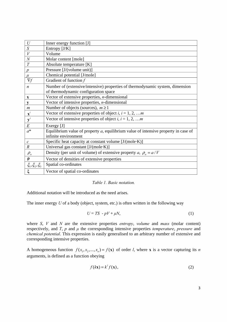
U Inner energy function [J] S Entropy [J/K] V Volume N Molar content [mole] T Absolute temperature [K] p Pressure [J/(volume unit)] μ Chemical potential [J/mole] ∇f Gradient of function f n Number of (extensive/intensive) properties of thermodynamic system, dimension

of thermodynamic configuration space x Vector of extensive properties, n-dimensional y Vector of intensive properties, n-dimensional m Number of objects (sources), 1≥m

ix Vector of extensive properties of object i, i = 1, 2, …m iy Vector of intensive properties of object i, i = 1, 2, …m

E Exergy [J] a* Equilibrium value of property a, equilibrium value of intensive property in case of

infinite environment c Specific heat capacity at constant volume [J/(mole·K)] R Universal gas constant [J/(mole·K)] ρa Density (per unit of volume) of extensive property a, /ρ =a a V ρ Vector of densities of extensive properties

1 2 3, ,ξ ξ ξ Spatial co-ordinates

ξ Vector of spatial co-ordinates

Table 1. Basic notation. Additional notation will be introduced as the need arises. The inner energy U of a body (object, system, etc.) is often written in the following way

U = TS - pV + μN, (1) where S, V and N are the extensive properties entropy, volume and mass (molar content) respectively, and T, p and μ the corresponding intensive properties temperature, pressure and chemical potential. This expression is easily generalised to an arbitrary number of extensive and corresponding intensive properties. A homogeneous function 1 2( , ,..., ) ( )=nf x x x f x of order l, where x is a vector capturing its n

arguments, is defined as a function obeying

( ) ( )lf k k f=x x ,

(2)

4

where k is any positive constant. A linearly homogeneous function is of unit order, l = 1. If

1 2

( ) , , ... , ∂ ∂ ∂= ∇ = ∂ ∂ ∂ n

f f ff

x x xy x is the gradient of such a function, we have:

1

( )( )

( )=

∂= =∂

n

ii i

ff x

x

xx yx .

(3)

Ever since the days of Josiah Willard Gibbs (1839-1903), (Gibbs, 1876, 1878), it has been recognised that the inner energy function is a linearly homogeneous function of the extensive properties of an object, that is with U(S, V, N), then the function obeys

( , , ) ( , , )=U kS kV kN kU S V N , (4)for any positive constant k. Hence, the intensive properties T, p and μ, may be interpreted as together forming the gradient of the inner energy function in thermodynamic configuration space

( )( , , ) , , , , μ∂ ∂ ∂ ∇ = = − ∂ ∂ ∂ U U U

U S V N T pS V N

,

(5)

and

( )( , , ) ( , , ) ( , , ) ( , , ) , , μ μ= ∇ = − = − +U S V N S V N U S V N S V N T p TS pV N ,

(6)

or in a more general form

( ) ( )= ∇ =U Ux x x xy . (7) where x and y are vectors capturing extensive and intensive properties, respectively. Eq. (7) is a generalisation of Gibbs’ Fundamental Equation (Gibbs, 1876, 1878). The classical formula given for the exergy content E of an object has the form (Ford, 1975, Eriksson et al., 1978, Wall, 1986):

( *) ( *) ( *)μ μ= − − − + −E T T S p p V N , (8) where T, p, and μ are the initial intensive properties of the source (object), *, * and *μT p the constant intensive properties of the environment, and S, V, N the initial extensive properties of the source, or in a more general form

( )( ) ( *)= ∇ − ∇E U Ux x x ,

(9)

where ( *)∇U x is a gradient vector holding the constant intensive properties of the environment. As an example, we may consider an ideal gas, the inner energy of which most often is written

5

=U cNT , (10) where c is the specific heat capacity (per mole and Kelvin at constant volume), and which obeys the ideal gas law:

=pV NRT , (11) where R is the universal gas constant. The standard formula (10) contains a mixture of intensive (T) and extensive (N) properties. But the inner energy may be written using only extensive properties (Grubbström, 1985, 2007)

/( ) / 1 /− += S cN R c R cU const e V N ,

(12) which is a linearly homogeneous function, where const is a positive undetermined constant. The gradient of U capturing its intensive properties is

/( ) / 1 /2

1 1, , 1− + ∇ = − + −

S cN R c R c R R S

U const e V NcN cV c N cN

,

(13)

from which we identify:

( )

/( ) / /

/( ) / 1 1 /

/( ) / /

( / ) ,

( / ) ,

( / ) / .μ

−

− − +

−

=

∇ = − = − = + −

S cN R c R c

S cN R c R c

S cN R c R c

T const c e V N

U p const R c e V N

const c e V N c R S N

(14)

Making the simple multiplications /( ) / 1 /( / ) − += S cN R c R cpV const R c e V N and =NRT

/( ) / /( / ) − =S cN R c R cNR const c e V N /( ) / 1 /( / ) − +S cN R c R cconst R c e V N , the ideal gas law obtains, and

taking /( ) / 1 /− += =S cN R c R ccNT const e V N U , we have the standard inner energy formula (10). So the inner energy function (12) includes both of these relations. 3: EXERGY FROM A SYSTEM OF FINITE OBJECTS Even if there is no environment, or if the environment is interpreted as an object with finite extension, the exergy concept may still be defined as the ideal maximum amount of mechanical work that a system of (at least two) objects may generate from the objects interacting (Grubbström, 1985, 2007). The formula for the exergetic content of m bodies in the system may then be written:

* * *

1 1 1 1

( ) ( ) ( ) ( )= = = =

= − = ∇ − ∇ = m m m m

i i i i i i i i

i i i i

E U U U Ux x x x x x

( )*

1

( ) ( )=

= ∇ − ∇m

i i i

i

U Ux x x ,

(15)

6

where ( )i iU x is the inner energy of body i having initial extensive properties ix , and *( )i iU x

the equilibrium inner energy of the same body when its extensive properties are *ix . Since the

sum of extensive properties are conserved for reversible processes *

1 1= =

= m m

i i

i i

x x , and the

intensive properties the same for all objects in equilibrium * *( ) ( )∇ = ∇i jU Ux x , i, j = 1, 2, …, m, the right-hand member obtains.

At equilibrium, we have * *

1 1

( )= =

∇ = ∇ = ∇

m mi j j

j j

U U Ux x x , for all i, so the exergy formula

(15) may conveniently be written:

1 1

( )= =

= ∇ − ∇

m m

i i i

i i

E U Ux x x ,

(16)

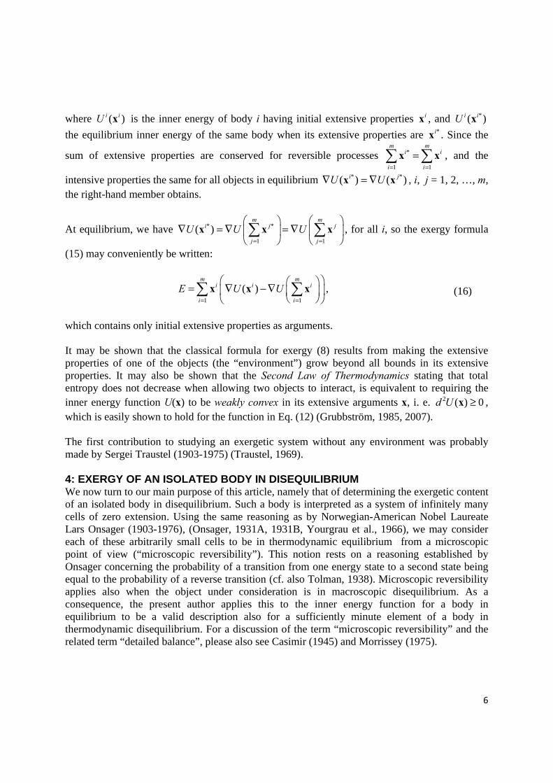
which contains only initial extensive properties as arguments. It may be shown that the classical formula for exergy (8) results from making the extensive properties of one of the objects (the “environment”) grow beyond all bounds in its extensive properties. It may also be shown that the Second Law of Thermodynamics stating that total entropy does not decrease when allowing two objects to interact, is equivalent to requiring the inner energy function U(x) to be weakly convex in its extensive arguments x, i. e. 2 ( ) 0≥d U x , which is easily shown to hold for the function in Eq. (12) (Grubbström, 1985, 2007). The first contribution to studying an exergetic system without any environment was probably made by Sergei Traustel (1903-1975) (Traustel, 1969). 4: EXERGY OF AN ISOLATED BODY IN DISEQUILIBRIUM We now turn to our main purpose of this article, namely that of determining the exergetic content of an isolated body in disequilibrium. Such a body is interpreted as a system of infinitely many cells of zero extension. Using the same reasoning as by Norwegian-American Nobel Laureate Lars Onsager (1903-1976), (Onsager, 1931A, 1931B, Yourgrau et al., 1966), we may consider each of these arbitrarily small cells to be in thermodynamic equilibrium from a microscopic point of view (“microscopic reversibility”). This notion rests on a reasoning established by Onsager concerning the probability of a transition from one energy state to a second state being equal to the probability of a reverse transition (cf. also Tolman, 1938). Microscopic reversibility applies also when the object under consideration is in macroscopic disequilibrium. As a consequence, the present author applies this to the inner energy function for a body in equilibrium to be a valid description also for a sufficiently minute element of a body in thermodynamic disequilibrium. For a discussion of the term “microscopic reversibility” and the related term “detailed balance”, please also see Casimir (1945) and Morrissey (1975).

7

Let us first consider the inner energy function of a body in equilibrium U(x). This function is linearly homogeneous. Defining the inner energy (volume) density as ( ) /ρ =U U Vx , where V is

one of the components belonging to x, this density becomes a homogeneous function of order zero:

0( ) ( ) / ( ) / ( )ρ ρ= = =U Uk U k kV kU x kV kx x x .

(17)

Let us further define the vector of densities by /= Vρ x . Setting k=1/V, ignoring temporarily that V is one of the variables, we obtain:

( / ) ( ) ( ) / ( )ρ ρ= = =U UV U kV Ux ρ ρ ρ . (18)

Hence, the inner energy density for a body in equilibrium is the inner energy function with the extensive properties exchanged for their corresponding densities, the density of volume necessarily being unity 1ρ =V .

For the special case of an ideal gas (remembering that 1ρ ≡V ), we may illustrate this by:

( )1 //( ) / 1 1 / ( / )/( / )/ /ρ +− − += = = =R cS cN R c R c S V cN VU U V const e V N const e N V

( )/( ) / 1 / , ,ρ ρ ρ ρ ρ ρ ρ− += =S Nc R c R cV N S V Nconst e U .

(19)

We introduce spatial co-ordinates contained in the vector ( )1 2 3, ,ξ ξ ξ=ξ , and divide the body

into small cells of size 1 2 3ξ ξ ξ=dV d d d . Each cell is located by its spatial co-ordinates ξ having

the density vector ( )ρ ξ at ξ and assumed to be in microscopic equilibrium according to Onsager’s hypothesis (Onsager, 1931A, 1931B, Yourgrau et al., 1966, pp. 35 ff.). The initial total extensive properties are thus contained in the vector:

1 2 3( ) ( ) ξ ξ ξ= = dV d d dξ ξ

x ρ ξ ρ ξ .

(20)

Generalising (16), we thus obtain the exergy content E for the body according to:

( ) 1 2 3 1 2 3( ) ( )ρ ξ ξ ξ ξ ξ ξ

= − =

UE d d d U d d dξ ξ

ρ ξ ρ ξ

( ) 1 2 3 1 2 3( ) ( )ξ ξ ξ ξ ξ ξ

= −

U d d d U d d dξ ξ

ρ ξ ρ ξ .

(21)

That exergy is a non-negative entity is clear from U being a weakly convex function of its extensive arguments. A function U(z), z being a point in the space considered, is defined to be weakly convex if

( ) ( ) ( )1 1 2 2 1 1 2 2+ ≥ +wU w U U w wz z z z .

(22)

8

where 1w and 1w are arbitrary non-negative weights adding up to unity. Letting ( )z ξ be a

vector-valued function of spatial co-ordinates ξ , we then have

( )( ) ( )( ) ( ) ( )( )1 1 2 2 1 1 2 2+ ≥ +wU w U U w wz ξ z ξ z ξ z ξ . The generalisation to a set of k points is

obvious:

( )( ) ( )1 1= =

≥

k k

i i i ii i

wU U wz ξ z ξ ,

(23)

with 1

1=

=k

ii

w , 0≥iw . Let the points represent individual volume elements each of size dV,

( ) =i iw dV wξ , ( )w ξ being a non-negative function with ( ) 1 2 3 1ξ ξ ξ =w d d dξ

ξ . For a

sufficiently large number k (small dV) , the two members of (23) keeping their relation then approach:

( ) ( )( ) ( ) ( )1 2 3 1 2 3ξ ξ ξ ξ ξ ξ

≥

w U d d d U w d d dξ ξ

ξ z ξ ξ z ξ .

(24)

With ( )w ξ chosen as a constant function ( ) 1/=w Vξ , and interpreting ( )z ξ as ( )ρ ξ , we obtain

( )( ) ( ) ( )1 2 3 1 2 3 1 2 3/ / /ξ ξ ξ ξ ξ ξ ξ ξ ξ

≥ =

U d d d V U d d d V U d d d Vξ ξ ξ

ρ ξ ρ ξ ρ ξ ,

(25)

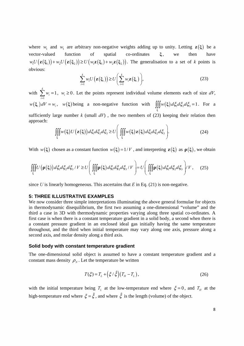
since U is linearly homogeneous. This ascertains that E in Eq. (21) is non-negative. 5: THREE ILLUSTRATIVE EXAMPLES We now consider three simple interpretations illuminating the above general formulae for objects in thermodynamic disequilibrium, the first two assuming a one-dimensional “volume” and the third a case in 3D with thermodynamic properties varying along three spatial co-ordinates. A first case is when there is a constant temperature gradient in a solid body, a second when there is a constant pressure gradient in an enclosed ideal gas initially having the same temperature throughout, and the third when initial temperature may vary along one axis, pressure along a second axis, and molar density along a third axis. Solid body with constant temperature gradient

The one-dimensional solid object is assumed to have a constant temperature gradient and a constant mass density ρN . Let the temperature be written

( )( )ˆ( ) /ξ ξ ξ= + −L H LT T T T ,

(26)

with the initial temperature being LT at the low-temperature end where 0ξ = , and HT at the

high-temperature end where ˆξ ξ= , and where ξ is the length (volume) of the object.

9

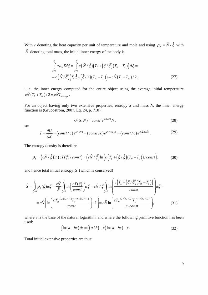
With c denoting the heat capacity per unit of temperature and mole and using ˆˆ /ρ ξ=N N with

N denoting total mass, the initial inner energy of the body is

( ) ( )( )( )ˆ ˆ

0 0

ˆ ˆˆ / /ξ ξ

ξ ξ

ρ ξ ξ ξ ξ ξ= =

= + − = N L H Lc Td c N T T T d

( ) ( )( )( ) ( )ˆ ˆ ˆˆ ˆ/ / 2 / 2ξ ξ ξ= + − = +L H L L Hc N T T T cN T T ,

(27)

i. e. the inner energy computed for the entire object using the average initial temperature

( )ˆ ˆ/ 2+ =L H averagecN T T cNT .

For an object having only two extensive properties, entropy S and mass N, the inner energy function is (Grubbström, 2007, Eq. 24, p. 710):

/( )( , ) = S cNU S N const e N ,

(28)so:

( ) ( ) ( ) ˆ ˆ/( ) /( )/( )/ / /ρ ρ ρ ξ∂= = = =∂

S N Sc cNS cNUT const c e const c e const c e

S.

(29)

The entropy density is therefore

( ) ( ) ( ) ( )( )( )( )ˆ ˆ ˆˆ ˆ/ ln ( ) / / ln / /ρ ξ ξ ξ ξ ξ= = + −S L H LcN cT const cN c T T T const ,

(30)

and hence total initial entropy S (which is conserved)

( )( )( )ˆ ˆ ˆ

0 0 0

ˆ/ˆ ( )ˆ ˆˆ( ) ln / lnˆ

ξ ξ ξ

ξ ξ ξ

ξ ξξρ ξ ξ ξ ξ ξξ= = =

+ − = = = =

L H L

S

c T T TcN cTS d d cN d

const const

( ) ( ) ( ) ( )/ / / /

ˆ ˆln 1 ln− − − − − −

= − = ⋅

H H L L H L H H L L H LT T T T T T T T T T T TH L H LcT T cT T

cN cNconst e const

,

(31)

where e is the base of the natural logarithm, and where the following primitive function has been used:

( ) ( )( ) ( )ln / ln+ = + + − a bz dz a b z a bz z .

(32)

Total initial extensive properties are thus:

10

( )( ) ( )ˆ / /

ˆ ˆ ˆˆ ˆ ˆˆ ( ) , , ln , ,ξ ξ ξ− − −

= = = ⋅

H H L L H LT T T T T TH LcT T

d S N cN Ne const

ξ

ξ

x ρ ξ .

(33)

The total equilibrium inner energy after maximal work extraction becomes

( ) ( )ˆ

ˆ / /ˆ/( ) ˆ ˆ( ) /ξ − − − = = H H L L H LT T T T T TS cn

H LU d const e N cNT T eξ

ξ

ρ ξ ,

(34)

which shows that the equilibrium temperature finalT after maximal work extraction is:

( ) ( )/ / /− − −= H H L L H LT T T T T T

final H LT T T e .

(35)

The initial inner energy density is obtained as

ˆ ˆ/( ) /( ) ˆˆ( , ) /ρ ρ ρ ξρ ρ ρ ρ ξ= = =S N Sc cNU S N NU const e const e N ,

(36)

so, using (36), the initial total inner energy may be obtained alternatively from:

( ) ( )( )( )( )ˆ ˆ ˆ

( )/( )

0 0 0

ˆ ˆˆ( ) / /ξ ξ ξ

ρ ξ ρ

ξ ξ ξ

ρ ξ ρ ξ ξ ξ ξ ξ= = =

= = + − = S NcU N L H Ld const e d c T T T N dρ ξ

( )ˆ / 2= +H LcN T T .

(37)

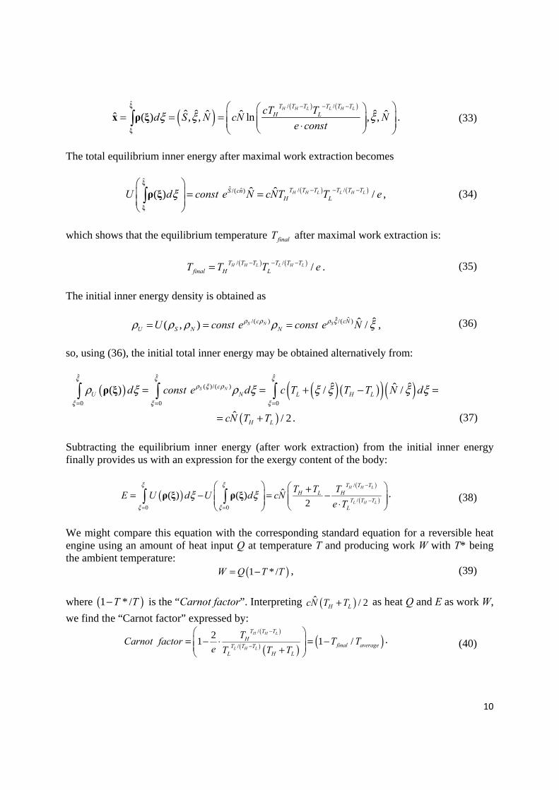
Subtracting the equilibrium inner energy (after work extraction) from the initial inner energy finally provides us with an expression for the exergy content of the body:

( )( )

( )

/

/0 0

ˆ( ) ( )2

ξ ξ

ξ ξ

ξ ξ−

−= =

+= − = − ⋅

H H L

L H L

T T TH L H

T T TL

T T TE U d U d cN

e Tρ ξ ρ ξ .

(38)

We might compare this equation with the corresponding standard equation for a reversible heat engine using an amount of heat input Q at temperature T and producing work W with T* being the ambient temperature:

( )1 * /= −W Q T T , (39)

where ( )1 * /−T T is the “Carnot factor”. Interpreting ( )ˆ / 2+H LcN T T as heat Q and E as work W,

we find the “Carnot factor” expressed by: ( )

( ) ( ) ( )/

/

21 1 /

−

−

= − ⋅ = − +

H H L

L H L

T T TH

final averageT T TL H L

TCarnot factor T T

e T T T.

(40)

11

So, as expected, finalT may be interpreted as the ambient temperature T*, and averageT as the input

temperature. If the two initial temperatures approach each other, the exergy of the body should approach zero, which is also shown by setting ( )/= −L H Lt T T T and taking

( )

( ) ( )( ) ( ) ( )/

1

/

1 1 1lim lim lim 1 1/ lim 1 1/ 1 1/

−+

−→ → →∞ →∞= = + = + + =

H H L

L H LH L H L

T T Tt tH

final L L LT T TT T T T t tL

TT t T t t T T

e e eT,

(41)

which makes E in (38) zero and the “Carnot factor” zero. Defining α from ( )1 α= +H LT T , i.e. 1 /α = t , where we accept that α might be negative, but

greater than -1, we find that the “Carnot factor” may be written as ( )( )1 ω α− e , where

( )( ) ( )( )( )1 1/( ) ln 2 1 / 2 /

αω α α α+= + + e . Analysing properties of ( )ω α results in ( )ω α always

being negative, except for 0α = , when (0) 0ω = , so the “Carnot factor” is positive and less than

unity for 0α ≠ and zero only for 0α = (the case of equal temperatures, =H LT T ). Hence, we are

assured that ≤final averageT T , as intuition suggests. If any other conclusion, then 0≥E in Eq. (21)

would have been violated. If the initial entropy density ( )ρ ξS instead would have been constant throughout the body,

ˆ( )ρ ξ ρ=S S , for all ξ , then total initial entropy becomes

ˆ

0

ˆ ˆˆ( )ξ

ξ

ρ ξ ξ ρ ξ=

= = S SS d ,

(42)

and total initial inner energy according to (36):

( ) ( )ˆ ˆ

ˆ ˆ ˆ ˆˆ /( ) /( )

0 0

ˆˆ ˆ( ) /ξ ξ

ρ ξ

ξ ξ

ρ ξ ξ ξ= =

= = S cN S cNU d const e N d const e Nρ ξ .

(43)

Temperature, according to (29), will take on the constant value T

( ) ( ) ( )ˆ ˆ ˆ ˆˆ ˆ/( ) /( ) /( ) ˆ( ) / / /ρ ρ ρ ξξ ∂= = = = =∂

S N Sc cN S cNUT const c e const c e const c e T

S,

(44)

for all ξ . Equilibrium total inner energy will then remain at the level

ˆ ˆ/( )ˆ ˆ ˆ= S cNcNT const Ne ,

(45)

12

and no mechanical work is possible to extract, i.e. E = 0. As a final consideration, we examine the equilibrium state if no work would be extracted, i. e. the case when inner energy is conserved and intensive properties are equalised throughout the

object. Conservation of inner energy implies ˆ ˆ *=averagecNT cNT , where T* is the equilibrium

temperature, which obviously must equal the initial average temperature. Furthermore, from Eq. (28), we obtain the equilibrium entropy S* as

( )ˆ* ln /= averageS cN cT const ,

(46)

so using (31) the (maximal) increase in entropy becomes:

( )( ) ( ) ( )/ /

/ 2ˆ ˆ ˆ* ln ln //− − −

+− = =

H H L L H L

H Laverage finalT T T T T T

H L

T TS S cN cN T T

T T e.

(47)

Ideal gas with constant pressure gradient and constant temperature

As a second illustration, we consider an ideal gas enclosed within a given one-dimensional volume with a constant pressure gradient, but having the same initial temperature throughout, say ˆ=T T . Let the pressure be written

( )ˆ( ) ( / )( )ξ ξ ξ= + −L H Lp p p p ,

(48)

where, as before, ξ is the one-dimensional spatial co-ordinate and ξ the spatial extension of the

object (the gas), and where Hp is the pressure at the high-pressure end, and Lp at the low-

pressure end. For an ideal gas, the inner energy function may be written according to (12), which by (19) means that the inner energy density is distributed as:

( ) ( )( )/ ( ) 1 /( ) ( , , ) ( ),1, ( ) ( )ρ ξ ρ ξρ ξ ρ ρ ρ ρ ξ ρ ξ ρ ξ += = = S Nc R cU S V N S N NU U const e .

(49)

But for an ideal gas in equilibrium we have =U cNT , so in microscopic equilibrium at the

location ξ having the temperature T the inner energy density becomes

ˆ( ) ( )ρ ξ ρ ξ=U Nc T ,

(50)

so the initial total inner energy will be

ˆ ˆ

0 0

ˆ ˆ ˆ( ) ( )ξ ξ

ξ ξ

ρ ξ ξ ρ ξ ξ= =

= = = initial U NU d cT d cNT ,

(51)

13

where N is the initial mass (moles), a total extensive property which will be conserved.

Apart from ξ , there are the initial extensive properties entropy S and mass N . Beginning with the latter, for an ideal gas with =pV NRT , at the co-ordinate ξ in microscopic equilibrium with

ˆ=T T , we must have ˆ( ) ( ) / ( )ρ ξ ξ=N p RT ,

(52)

so

( ) ( )ˆ ˆ ˆ

0 0 0

ˆ1 1 ˆˆ ( ) ( ) ( / )( )ˆ ˆ ˆ2

ξ ξ ξ

ξ ξ ξ

ξρ ξ ξ ξ ξ ξ ξ ξ

= = =

+= = = + − = H L

N L H L

p pN d p d p p p d

RT RT RT,

(53)

which by (51) shows the initial average pressure ( ) / 2= +average H Lp p p as an argument yielding

the initial inner energy for the object as ( ) ˆ/ ξ=initial averageU c R p .

Concerning total initial entropy the computations are more lengthy. Taking the logarithm of (49) and (50), the entropy density is found to be

( ) ( )( )ˆ( ) ( ) ln / / ln ( )ρ ξ ρ ξ ρ ξ= − =S N Nc cT const R c

( )( ) ( ) ( ) ( )( )ˆ ˆ/ /ˆln / / ln

ˆ ˆ

ξ ξ ξ ξ + − + − = −

L H L L H Lp p p p p pc cT const R c

RT RT. (54)

So total initial entropy S (which is conserved) is

( )( )2 2 2 2 2 2

ˆ/

/( ) /( )1/2

0

ˆˆ ˆ ˆ( ) ln /

ˆ 2

ξ

ξ

ξρ ξ ξ − − −

=

+= = H H L L H Lc R

p p p p p pH LS H L

p pS d e RT cT const p p

T,

(55)

where the following primitive function has been used:

( )2

ln ln 1/ 22

= −z

z z dz z .

(56)

Total inner energy at equilibrium after maximal work extraction then becomes:

( ) ( )2 2 2 2/(2 )

ˆ ˆ/( ) / 1 / 1 /( )ˆ

ˆ ˆ ˆˆ ˆ, ,ξξ ξ −− + +−= = L H H L

RR cp pS cN R c R c R cc p p

L H average

c eU S N const e N p p p

R, (57)

where, as before, averagep is initial average pressure.

According to (21), the exergy of this ideal gas in disequilibrium is therefore:

14

( ) ( )2 2 2 2

ˆ 1 //(2 ) ( )

0

ˆ ˆ ˆˆ ˆ ˆ( ) , , ( / )2

ξ

ξ

ρ ξ ξ ξ ξ+

− −

=

+ = − = − = L H H L

R R cp pR c H Lc p p

U L H

p pE d U S N cNT c R e p p

= ( )2 2 2 2/(2 ) /( )ˆ

1ξ − −

−

L H H L

Rp pR c R cc p p

average L H average

cp e p p p

R. (58)

The final pressure after maximal work extraction will be:

ˆ ˆ/( ) 1 / 1 /ˆ ˆ ˆ ˆˆ ˆ( , , ) / ( / )ξ ξ ξ − − += −∂ ∂ = =S cN R c R cfinalp U S N R c const e N

2 2

2 2 2 2

/

( ) ( )1 / 1/2−

− −+ =

L H

H L H L

R cp p

p p p pR caverage L Hp e p p ,

(59)

from which we find

2 2

2 2 2 2( ) ( )1/2 / 1 /−

− − − −=L H

H L H L

p p

p p p p c R c RL H final averagee p p p p , so exergy may be written:

( ) ( )ˆ/ 1 /ξ= −average final averageE c R p p p .

(60)

Again, we may interpret a “Carnot factor”, in this case as:

( )1 /= − final averageCarnot factor p p .

(61)

Since exergy is non-negative, we find ≤final averagep p as expected. From the pressure being the

same throughout the body after work extraction, the final temperature must obey ˆ ˆξ =final finalp NRT , which, using (59), gives the final temperature finalT :

2 2

2 2 2 2

/

( ) ( )1 /ˆ

ˆ /ˆ

ξ −− −+

= =

L H

H L H L

R cp p

p p p pR cfinal average L H final averageT p e p p Tp p

RN,

(62)

which also shows the intuitive result ˆ≤finalT T .

To complete this example, we examine the situation arising from a case when no work is extracted and the system is moved into equilibrium generating a maximal entropy increase. Then

=initial finalU U , so ˆ ˆcNT equals ( )ˆ*/ / 1 /ˆ ˆξ − +S cN R c R cconst e N , where S* is final entropy. From (53), we

thus obtain: 1 /

1 /

ˆˆ* ln

ˆξ +

+

=

R caverage

R c

c pS cN

const RN.

(63)

Subtracting initial entropy S , using (55) and (59), yields the entropy increase as:

15

( )ˆ ˆ* ln /− = average finalS S cN p p ,

(64)

which may be compared with the similar expression in our first example (47). If the two extreme pressures initially are equal, =H Lp p , one would expect the exergy content to

be zero, which is also shown by using ( )/= −L H Lt p p p and letting → ∞t :

( ) ( )2 2

2 2 2 21 /

( ) ( )/(2 )lim lim2

+−− −

→ →

+ = =

L H

H L H L

H L H L

R p R p R cc p p c p pR c H L

final L Hp p p p

p pp e p p

( ) ( ) ( )( )2

2 /(2 )2 /(1 2 )/(2 ) 1 2lim / (1 ) lim / (1 )

++

→∞ →∞= + = +

R cRtt tR c c t

H Ht t

e p t t p e t t =

=

( )( ) ( )2

/(2 )/(2 )

2

1 2lim 1 1/lim 1 1/ + →∞

→∞

= = + +

R cR c

H H Htt

t tt

e ep p p

tt

.

(65)

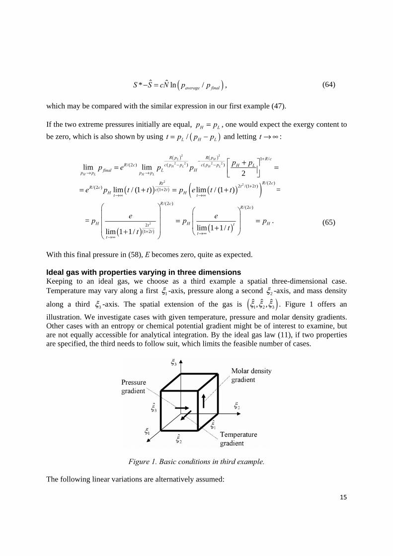
With this final pressure in (58), E becomes zero, quite as expected. Ideal gas with properties varying in three dimensions Keeping to an ideal gas, we choose as a third example a spatial three-dimensional case. Temperature may vary along a first 1ξ -axis, pressure along a second 2ξ -axis, and mass density

along a third 3ξ -axis. The spatial extension of the gas is ( )1 2 3ˆ ˆ ˆ, ,ξ ξ ξ . Figure 1 offers an

illustration. We investigate cases with given temperature, pressure and molar density gradients. Other cases with an entropy or chemical potential gradient might be of interest to examine, but are not equally accessible for analytical integration. By the ideal gas law (11), if two properties are specified, the third needs to follow suit, which limits the feasible number of cases.

Figure 1. Basic conditions in third example. The following linear variations are alternatively assumed:

16

Along 1ξ -axis (temperature gradient)

( ) ( )( )1 2 3 1 1, , /ξ ξ ξ ξ ξ= + −L H LT T T T , (66)

along 2ξ -axis (pressure gradient)

( ) ( )( )( )1 2 3 2 2, , /ξ ξ ξ ξ ξ= + −L H Lp p p p , (67)

along 3ξ -axis (molar density gradient)

( ) ( )( )1 2 3 3 3, , /ρ ξ ξ ξ ρ ξ ξ ρ ρ= + −N NL NH NL , (68)

where subscripts with “H” refer to values at high property ends, and “L” at low property ends. For an ideal gas we always have ( ) ( )1 2 3 1 2 3, , ( / ) , ,ρ ξ ξ ξ ξ ξ ξ=U c R p , so total initial inner energy

in cases of a constant pressure gradient will then be:

( ) ( ) ( )( )1 2 3 1 2 3

1 2 3 3 2 1 2 2 3 2 1

, , , ,

ˆ, , / /ξ ξ ξ ξ ξ ξ

ρ ξ ξ ξ ξ ξ ξ ξ ξ ξ ξ ξ= = + − = initial U L H LU d d d c R p p p d d d

( ) ( )1 2 3 1 2 3ˆ ˆ ˆ ˆ ˆ ˆ/ /

2ξ ξ ξ ξ ξ ξ+= =L H

average

p pc R c R p ,

(69)

where, as before, ( ) / 2= +average L Hp p p .

Case I. Given constant temperature and pressure gradients As a first case we assume a temperature and pressure gradient (66) and (67). Starting by

calculating the total molar content N , from ( / )ρ =Nc T c R p , we find the molar density to be

( )( )( )( )

( )( )( )2 2

1 2 3

1 1

ˆ/, ,

ˆ/

ξ ξρ ξ ξ ξ

ξ ξ

+ −=

+ −

L H L

N

L H L

p p p

R T T T,

(70)

which gives

( )( )( )( )( )( )

( )( )( )( )( )( )

1 2

1 2

ˆ ˆ2 2 2 2

1 2 3 3 2 1

0 01 1 1 1

ˆ ˆ/ /ˆˆ

ˆ ˆ/ /

ξ ξ

ξ ξ

ξ ξ ξ ξξ ξ ξ ξ ξ ξ

ξ ξ ξ ξ= =

+ − + −= = =

+ − + −

L H L L H L

L H L L H L

p p p p p pN d d d d d

R T T T R T T Tξ

( )( )( )( )

( )1

1

ˆ

1 2 313 2

0 1 1

ˆ ˆ ˆ ln /ˆ ˆˆ2 /

ξ

ξ

ξ ξ ξξξ ξξ ξ=

−= =

−+ − averageH L H L

H LL H L

pp p T Td

R T TR T T T.

(71)

Secondly, the entropy density ρS is given by taking the logarithm of (19):

17

( ) ( )1 2 3, , ( ) ln( / ( )) ln (1 / ) lnρ ξ ξ ξ ρ ρ= + − + =S N Nc c constR p R c

/( / ) (1 / )ln − +

=

R cR c R ccp cR

p TRT const

,

(72)

where p and T have given distributions in space. So, after lengthy calculations, total initial

entropy S is obtained as:

/( / ) (1 / )2

2 1 1 2 31

( )ˆ ln ( ) ( )( )

ξ ξ ξ ξ ξ ξξ

− + = =

R cR c R ccp cR

S p T d d dRT constξ

( ) ( ) ( )( ) ( ) ( )2 2

2 2 2 2

/

1 / /2/1 2 3ˆ ˆ ˆ ln /

ln /ξ ξ ξ −

− −+

= −

H L

H L H L

R cp p

p p p pR cH L R caverage H L H L

H L

T Tcp c const R e T T p p

R T T.

(73)

Inserting S , N and 1 2 3ˆ ˆ ˆξ ξ ξ=V into the inner energy function (12) gives us the inner energy after

work extraction:

( ) ( ) ( ) ( )2 2

2 2 2 2

/1 /

1 2 3

ln /ˆ ˆ ˆ/ ξ ξ ξ+ −

− − = −

H L

H L H L

R cp pR c

p p p pH L H Lfinal average average H L

H L

T T T TU c R e p p p p

T T.

(74)

So, by subtracting finalU from initialU in (69), exergy becomes

( ) ( ) ( ) ( )2 2

2 2 2 2

/1 /

1 2 3

ln /ˆ ˆ ˆ/ 1ξ ξ ξ+ −

− −

= − −

H L

H L H L

R cp pR c

p p p pH L H Laverage average H L

H L

T T T TE c R p e p p p

T T,

(75)

which also shows the corresponding “Carnot factor”. Further final equilibrium properties finalT and finalp after work extraction are found from

ˆ=final finalU cNT and 1 2 3ˆ ˆ ˆ ˆξ ξ ξ =final finalp RNT :

( ) ( ) ( ) ( )2 2

2 2 2 2

//

(1 / ) ln / −+ − − = −

H L

H L H L

R cp pR c

R c p p p pH Lfinal H L average H L

H L

T TT e T T p p p

T T.

(76)

( ) ( ) ( )2 2

2 2 2 2

/1 /

ln /+ −

− − = −

H L

H L H L

R cp pR c

p p p pH Lfinal H L average H L

H L

T Tp e T T p p p

T T.

(77)

18

Hence the “Carnot factor” may be written ( )1 /− final averagep p (which is the same as in (61)) and

exergy becomes:

( ) ( )1 2 3ˆ ˆ ˆ/ 1 /ξ ξ ξ= −average final averageE c R p p p ,

(78)

which is the 3D equivalent of (60). If instead of work extraction, the ideal gas had been brought to rest in equilibrium preserving its

inner energy, we have ˆ *=initialU cNT and 1 2 3ˆ ˆ ˆ ˆ* *ξ ξ ξ =p NRT with T* and p* being equilibrium

temperature and pressure, which by (69) and (71) yields:

( ) ( )* / ln /= −H L H LT T T T T ,

(79)

* = averagep p .

(80)

If HT and LT were equal, l’Hôpital’s rule applied to (79) shows * = =L HT T T , and if Hp and Lp

were equal, then * = =L Hp p p .

Other cases Since the derivations of the other cases are very similar to Case I, we refrain from reporting details and conclude by listing results for all three cases in Tables 2-8. In the formulae, we use

1 2 3ˆ ˆ ˆˆ ξ ξ ξ=V for the fixed volume.

Case Variations Given parameter values Equations I Temperature and pressure ,L HT T , ,L Hp p (66), (67) II Pressure and molar density ,L Hp p , ,ρ ρNL NH (67), (68) III Temperature and molar density ,L HT T , ,ρ ρNL NH (66), (68)

Table 2. Description of three cases treated.

Case Total initial mass N

I ( ) ( ) ( ) ˆ1/ ln / / −average H L H LR p T T T T V

II ˆρNaverageV

III ˆρNaverageV

Table 3. Total initial mass.

19

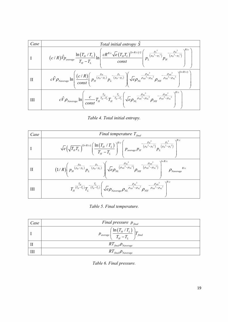
Case Total initial entropy S

I ( ) ( ) ( )( )( ) ( )

2 2

2 2 2 2

/1 / /2/ln /ˆ/ ln+ −

− −

−

L H

H L H L

R cp pR cR c

p p p pH L H Laverage L H

H L

T T cR e T Tc R Vp p p

T T const

II ( ) ( ) ( )

2 2

2 2 2 2

(1 / )

/ˆ lnρ ρ

ρ ρ ρ ρρ ρ ρ

+−−

− − − −

NL NHH L

H L H L NH NL NH NL

R cp p

p p p pNaverage H L NL NH

c RcV p p e

const

III

2 2

2 2 2 2

/

ˆ lnρ ρ

ρ ρ ρ ρρ ρ ρ−−

− −− −

NL NHH L

NH NL NH NLH L H L

R cT T

T T T TNaverage H H NL NH

ccV T T e

const

Table 4. Total initial entropy.

Case Final temperature finalT

I ( ) ( ) ( ) ( )2 2

2 2 2 2

//

(1 / ) ln / −+ − −

−

H L

H L H L

R cp pR c

R c p p p pH LH L average H L

H L

T Te T T p p p

T T

II ( ) ( ) ( ) ( ) ( )2 2

2 2 2 2

1 /

/1 /

ρ ρρ ρ ρ ρρ ρ ρ

+−− − −− −

NL NHH L

NH NL NH NLH L H L

R cp p

p p p p R cH L NL NH NaverageR p p e

III ( ) ( )2 2

2 2 2 2

/ρ ρ

ρ ρ ρ ρρ ρ ρ−−

− − − −

NL NHH L

H L H L NH NL NH NL

R cT T

T T T TH L Naverage NL NHT T e

Table 5. Final temperature.

Case Final pressure finalp

I ( )ln /

−

H Laverage final

H L

T Tp T

T T

II ρfinal NaverageRT

III ρfinal NaverageRT

Table 6. Final pressure.

20

Case Total initial inner energy

initialU Total final inner energy

finalU Exergy

E

I ( ) ˆ/ averagec R p V ( ) ˆ/ finalc R p V ( )( ) ˆ/ −average finalc R p p V

II ( ) ˆ/ averagec R p V ( ) ˆ/ finalc R p V ( )( ) ˆ/ −average finalc R p p V

III ˆρaverage NaveragecT V ˆρfinal NaveragecT V ( ) ˆρ−average final Naveragec T T V

Table 7. Total initial and final inner energy, exergy.

For the situation that inner energy would be preserved and the gas brought to thermodynamic equilibrium without any work extraction, Table 8 presents relevant formulae:

Case Entropy increase

( )ˆ*−S S

Equilibrium temperature T*

Equilibrium pressure p*

I ( )( ) ( )ˆ/ / ln /final final average finalc R p T V p p ( ) ( )/ ln /−H L H LT T T T averagep

II ( )ˆ ln /ρNaverage average finalc V p p ( )( )1/ / ρaverage NaverageR p averagep

III ( )ˆ ln /ρNaverage average finalc V T T averageT ρNaverage averageR T

Table 8. Entropy increase, equilibrium temperature and pressure in cases of no work extraction. As a final consideration, we may assume an intermediate situation between the extremes of no work output (Table 8) and maximal work output (exergy), i. e. W, 0 < <W E . Then, limiting ourselves to Case III, with ΔS being the entropy increase, we have

( )ˆ/( )ˆ 1 /ρρ Δ= − averageS c Vaverage Naverage final averageW cT V e T T ,

(81)

showing the inverse relation between work output and entropy generation. With a zero entropy increase 0Δ =S , then work output is exergy (cf. Table 7), and with no work output, the entropy increase is maximal (Table 8, first column). It should be noted that finalT in (81) is the expression

from Table 5 and not the final temperature if the work output were less than E. Sensitivity analyses by examining effects from adjusting given parameters in (66)-(68) are easily performed, but left to the reader. CONCLUSIONS AND FURTHER RESEARCH After having summarised previous related findings in the first three sections of this paper, we derived general formulae for the exergetic content of an isolated object, which is in thermodynamic disequilibrium, meaning that the intensive properties of the body are distributed heterogeneously in space. This led to the basic formula (21) in Section 4. Our developments have

21

relied heavily on the validity of Gibbs’ Fundamental Equation, stating that the inner energy function is linearly homogeneous in its extensive variables, and on the notion of Onsager assuming that an infinitely small portion of an object may be considered to be in microscopic thermodynamic equilibrium. Two one-dimensional examples and one three-dimensional example were provided in Section 5, on the one hand, a solid object with an initial constant temperature gradient, on the second, an ideal gas with a constant pressure gradient but having a homogeneous temperature distribution. In the third example, an ideal gas was considered with intensive properties varying along three axes. As side results from these examples, formulae have been provided for final state temperatures and pressures in the examples as well as comparisons with an alternative transition to equilibrium without work extraction. Of course the results obtained are theoretical, and neither explain how the mechanical work is to be extracted nor what losses are expected. For instance, in the first example one could imagine a heat engine taking heat from a hot point and delivering it to a cold point, the difference in flows being the work output. But the hot and cold spots would probably all the time be moving in a complicated way. And one would also expect a simultaneous internal transfer of heat within the body due to conduction, necessarily destroying exergy. But exergy is the upper bound of work extracted, and although it is unattainable in practice, this measure still has a concrete physical meaning. In future research there could be several avenues of approach opening themselves up for investigation. A first question might be to study a body in disequilibrium, when surrounded by an environment with constant intensive properties, and how the exergy formulae then are affected. But the real challenge would be met when combining disequilibrium exergetics with empirical laws like Fourier’s Law, Hartley-Fick’s Law, Ohm’s law, etc., by which the fluxes, at least as a first approximation, are proportional to corresponding thermodynamic gradients with densities of extensive properties as arguments. Then extreme generalisations of finite time thermodynamics of the Curzon-Ahlborn type (Curzon & Ahlborn, 1975) might not be far off to reach. ACKNOWLEDGEMENT The author gratefully recognises the valuable comments given by Professor Lars-Erik Andersson, Department of Mathematics, Linköping Institute of Technology. REFERENCES Casimir, H. B. G. (1945). On Onsager's Principle of Microscopic Reversibility, Reviews of Modern Physics, 17 (2-3), pp. 343-350. Curzon, F. L. & Ahlborn, B. (1975). Efficiency of a Carnot engine at maximum output, American Journal of Physics, 43(1), 22-24. Eriksson, B., Eriksson, K.-E. & Wall, G. (1978). Towards an Integrated Accounting of Energy and Other Natural Resources, Dept of Theoretical Physics, Chalmers University of Technology, January.

22

Ford, K. W., et al., (Eds), (1975). Efficient Use of Energy, AIP Conference Proceedings No 25, American Institute of Physics, New York, N.Y. Gibbs, J. W. (1876). On the Equilibrium of Heterogeneous Substances, Transactions of the Connecticut Academy, III, 108-248 (October, 1875-May, 1876), 343-524 (May, 1877-July, 1878). Gibbs, J. W. (1878). On the Equilibrium of Heterogeneous Substances: Abstract by the Author, American Journal of Science, XVI, 441-458. Grubbström, R. W. (1985). Towards a generalized exergy concept. In: van Gool W. & Bruggink J. J. C., (Eds). Energy and time in the economic and physical sciences. Amsterdam: North-Holland, 41–56. Grubbström, R. W. (2007). An attempt to introduce dynamics into generalised exergy considerations, Applied Energy, 84, 701–718. Kline, S. J. (1999). The Low-Down on Entropy and Interpretive Thermodynamics, La Cañada, CA: DCW Industries. Morrissey, B. W. (1975). Microscopic Reversibility and Detailed Balance. An overview, Journal of Chemical Education, 52(5), pp. 296-298. Onsager, L. (1931A). Reciprocal relations in irreversible processes. I, Physical Review, 37, 405-436, Feb. Onsager, L. (1931B). Reciprocal relations in irreversible processes. II, Physical Review, 38, 2265-2279, Dec. Rant, Z. (1956). Exergie, Ein neues Wort für "technische Arbeitsfähigkeit", Forschung auf dem Gebiete des Ingenieurswesens, 22, pp. 36-37. Rosen, M. A., Dincer, I. & Kanoglu, M. (2008). Role of exergy in increasing efficiency and sustainability and reducing environmental impact, Energy Policy, 36, 128–137. Tolman, R. C. (1938). The Principles of Statistical Mechanics, London: Oxford University Press, 152-165. Traustel, S. (1969). Die Arbeitsfähigkeit eines System-Paares, Brennstoff-Wärme-Kraft, 21(1), 2-5. Wall, G. (1986). Exergy - A Useful Concept, Physical Resource Theory Group, Chalmers University of Technology, Gothenburg.

23

Wall, G., (1997). Bibliography on Exergy, from http://users.ntua.gr/rogdemma/Bibliography%20on%20Exergy.pdf. Yourgrau, W., van der Merwe, A. & Raw, G. (1966). Treatise on Irreversible and Statistical Thermophysics, Macmillan, New York.