on the estimation and properties of logistic regression ... · pdf fileon the estimation and...

IOSR Journal of Mathematics (IOSR-JM)

e-ISSN: 2278-5728, p-ISSN: 2319-765X. Volume 10, Issue 4 Ver. III (Jul-Aug. 2014), PP 57-68 www.iosrjournals.org

www.iosrjournals.org 57 | Page

On the Estimation and Properties of Logistic Regression

Parameters

1Anthony Ngunyi,

2Peter Nyamuhanga Mwita, 2 Romanus O. Odhiambo

Abstract: Logistic regression is widely used as a popular model for the analysis of binary data with the areas

of applications including physical, biomedical and behavioral sciences. In this study, the logistic regression model, as well as the maximum likelihood procedure for the estimation of its parameters, are introduced in

detail. The study has been necessited with the fact that authors looked at the simulation studies of the logistic

models but did not test sensitivity of the normal plots. The fundamental assumption underlying classical results

on the properties of MLE is that the stochastic law which determines the behaviour of the phenomenon

investigated is known to lie within a specified parameter family of probability distribution (the model). This

study focuses on investigating the asymptotic properties of maximum likelihood estimators for logistic

regression models. More precisely, we show that the maximum likelihood estimators converge under conditions

of fixed number of predictor variables to the real value of the parameters as the number of observations tends to

infinity.We also show that the parameters estimates are normal in distribution by plotting the quantile plots and

undertaking the Kolmogorov -Smirnov an the Shapiro-Wilks test for normality,where the result shows that the

null hypothesis is to reject at 0.05% and conclude that parameters came from a normal distribution.

Key Words: Logistic, Asymptotic, Normality, MRA(Multiple Regression Analysis)

I. Introduction Regression analysis is one of the most useful and the most frequently used statistical methods [24, 3].

The aim of the regression methods is to describe the relationship between a response variable and one or more

explanatory variables. Among the different regression models, logistic regression plays a particular role. The

basic concept, however, is universal. The linear regression model is, under certain conditions, in many

circumstances a valuable tool for quantifying the effects of several explanatory variables on one dependent

continuous variable. For situations where the dependent variable is qualitative, however, other methods have

been developed. One of these is the logistic regression model, which specifically covers the case of a binary (dichotomous) response. [6] discussed an overview of the development of the logistic regression model. He

identifies three sources that had a profound impact on the model: applied mathematics, experimental statistics,

and economic theory. [?] also provided details of the development on logistic regression in different areas. He

states that, “Sir [5] introduced many statisticians to logistic regression through his 1958 article and 1970 book,

“The Analysis of Binary Data”. However, logistic regression is widely used as a popular model for the analysis

of binary data with the areas of applications including physical, biomedical, and behavioral sciences.

In this study, the logistic regression models, as well as the maximum likelihood procedure for the

estimation of their parameters, are introduced in detail. Based on real data set, an attempt has been made to

illustrate the application of the logistic regression model.

Simulation is used in the study since it involves construction of complicated integrals that do not exists

in a closed form that can be evaluated. Simulation methods can be used to evaluate it to within acceptable degrees of approximation by estimating the expectation of the mean of a random sample.

II. Literature Review The method of maximum likelihood is the estimation method used in the logistic regression models,

however, two other methods have been and may still be used for estimating the coefficient . These methods are

the least squares and the discriminant function analysis. The linear model approach of analysis of categorical

data proposed by Grizzle et al.(1969) used estimaton based on NonLinear Weighted S(NLWS). They

demostrated that logistic model can be handled by the method of maximum likelihood using an iterative

reweighted least squares algorithm. The discriminant approach to estimation of the coefficients is of historical importance as popularized by [4]. [14] compared the two methods when the model is dichotomous and

1 Dedan Kimathi University of Technology Kenya

P.O BOX 657-10100, Nyeri 2 Jomo Kenyatta University of Agriculture & Technology Kenya

P.O BOX 62000-00200, Nairobi

On the Estimation and Properties of Logistic Regression Parameters


concluded that the discriminat function was sensitive to the assumption of normality. In particular, the

estimation of the coefficient for the nonnormal distributed variables are biased away from zero, when the

coefficient is in fact different from zero. This implies that for the dichotomous independent variable the

discrimnant function will overestimate the magnitude of the coefficient.

According to [13], the fact concerning the interpretability of the coefficients is the fundamental reason

why logistic regression has proven such a powerful analytic tool for epidemiologic research. At least, this

argumentation holds whenever the explanatory variables x are quantitative. [9] investigate the asymptotic

properties of various discrete and qualitative response models (including logit model) and provided conditions

under which the MLE has its usual asymptotic properties, that is, the p -vector of coefficients of linear

combinations ,x has to be estimated from a finite sample of n observations. The method of analysis of

generalized linear models can be used since logistic models are sub-category [17].

[11] established that the maximum likelihood estimators are the best asympotically and strong

consistent estimators of the logit model, other estimators have been suggested for logit model including the

minimum divergent estimator which are generalization of maximum likelihood and are also consistent and

asymptotically normal [20].

[25] discussed the inconsistency of the generalized method of moments estimator of qualitative models with random regressors and suggested a suitable modification in case of the probit and not the logit.

In the parameter estimation and inference in statistics, maximum likelihood has many optimal

properties in estimation: sufficiency (complete information about the parameter of interest contained in its

estimation); consistency (true parameter value that generated the data recovered asymptotically, i.e. data of

sufficiently large samples); efficiency (lowest possible variance of parameter estimates achieved asymptotically)

and parameterization invariance. The asymptotic normality of the maximum likelihood in logistic regression

models are also found in [18] and [19]. [18] presents regularity conditions for a multinomial response model

when the logit link is used. [19] presents regularity conditions that assure asymptotic normality for the logit link

in binomial response models and further verifies that his conditions are equivalent to those of [18]. [7] discuss

the asymptotic distribution of the MLE for constructing confidence intervals and conducting tests of

hypotheses.[12] prove that the MLE is asymptotically normal in this setting as long as certain regularity

conditions are satisfied

2.1 Logistic function

The function has been discussed by many reseachers like [10]. It is given by;

gexp

gexpgf

1

)(=

gexp1

1= (1)

when modelling a bernoulli random variable with multivariables, one directly models the probabilities

of group membership, as follows;

jij

d

j

xexp

xXYP

1=

01

1==|1= (2)

where g in 1 is given by

dd XXXXg 11221110=; (3)

To illustrate, the applicability of the logistic function, the bold curve in the figure 0 shows that the

logistic function puts more weight on the tails than the normal distribution.



Figure 1: Standardized Normal and Logistic CDF’s

The logistic model is bounded between zero and one, this property estimates the possibility of getting

estimated or predicted probabilities outside this range which would not make sense. Also with a proper

transformation, one can get a linear model from the logistic function. [10] uses the logit function of the

Bernoulli distributed response variable. Transforming 2 as in [10] we have ;

xXYP

xXYPlogxXYPLogit e

=|1=1

=|1===|1=

ijj

d

j

ijj

d

j

e

Xexp

Xexp

log

1=

0

1=

0

1

1

=

ijj

d

j

e Xexplog 1=

0=

ijj

d

j

X 1=

0= (4)

the function 4 is a generalized linear model (GLM) with d independent variables.

The motivation to the use of logistic model is that it follows the properties of the GLM. Lets define the

hypothetical population proportion of cells for which 1=Y as xXYP =|1== . Then the theoretical

proportion of cells for which 0=Y is xXYP =|0==1 . We estimate by the sample proportions

of cells for which 1=Y . In the GLM context, it is assumed that there exists a set of predictor variables,

dXXX 11211 ,,, , that are related to Y and therefore provides additional information for estimating Y . For

mathematical reasons of additivity and multiplicity, logistic model is based on linear model for the log odds in

favour of 1.=Y

ijj

d

ji

ie Xlog

1=

=1

thus

ijj

d

j

i X 0=

=

where d of unknown parameters.

The logistic regression (logit link)



i

i

iei logitlogg

=

1=

and

iigg =1

thus the inverse of the logit function in terms of ;X is given by;

jij

d

j

i

xexp

Xg

1=

0

1

1

1==;

This model can be rewritten as

ijj

d

j

i Xlogit 0=

=)(

III. Methodology

3.1 Maximum Likelihood Estimation of the Parameter β

[10] pointed out that estimating the function xXYP =|1= in 1 is equivalent to estimating the

function ;Xg 2. Parametric estimation of ;Xg can be found in [15], [21] and [22] among other

authors, they used the maximum likelihood estimation method. As they pointed out, one first defines the

likelihood function. For the Bernoulli distribution case we have

iy

iy

n

i

xXYPxXYPXYL

1

1=

=|1=1=|1==;,

So, taking the logarithm and upon simplification we have

;1;(=;, XgexplogXgyXYL ei (5)

The regularity conditions requires that the MLEs of satisfies the usual consistency and asymptotic

normality properties [1, 11].

The optimization of the function in 5 with respect to the unknown vector requires iterative

techniques since first derivative is nonlinear in ̂ and has no simple analytical solution for ̂ [16].

ij

ijj

d

i

ijj

d

i

iiji

d

i

' x

Xexp

Xexp

nxyXYL

1=

1=

1=1

=;, (6)

ijiiiji

d

i

xnxy 1=

= (7)

In matrix form, 7 can be rewritten in the form;

Xii

n

i

' yXYL 1=

=;, (8)

The equation,



ijj

d

i

ijj

d

i

i

Xexp

Xexp

1=

1=

1

=

is strictly increasing function (monotone) of j and approaches 0 as j and approaches n as

.j The second derivative of 6 is strictly negative for all sj ' and as such the solution is a maximum

[2, 23].

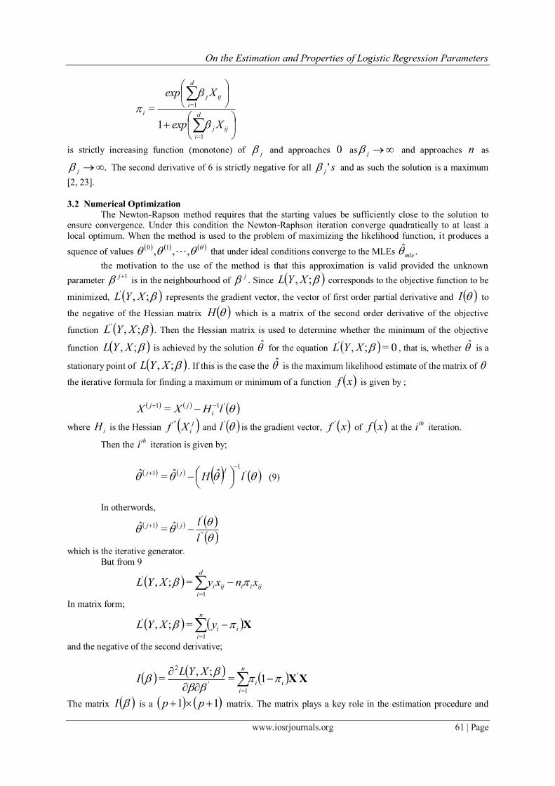
3.2 Numerical Optimization

The Newton-Rapson method requires that the starting values be sufficiently close to the solution to ensure convergence. Under this condition the Newton-Raphson iteration converge quadratically to at least a

local optimum. When the method is used to the problem of maximizing the likelihood function, it produces a

squence of values ,,, 10 that under ideal conditions converge to the MLEs .ˆ

mle

the motivation to the use of the method is that this approximation is valid provided the unknown

parameter 1j is in the neighbourhood of

j . Since ;, XYL corresponds to the objective function to be

minimized, ;, XYL' represents the gradient vector, the vector of first order partial derivative and I to

the negative of the Hessian matrix H which is a matrix of the second order derivative of the objective

function ;, XYL''. Then the Hessian matrix is used to determine whether the minimum of the objective

function ;, XYL is achieved by the solution ̂ for the equation 0=;, XYL', that is, whether ̂ is a

stationary point of ;, XYL . If this is the case the ̂ is the maximum likelihood estimate of the matrix of

the iterative formula for finding a maximum or minimum of a function xf is given by ;

'

i

jj lHXX 11 =

where iH is the Hessian j

i

'' Xf and 'l is the gradient vector, xf ' of xf at the

thi iteration.

Then the thi iteration is given by;

'

jjj lH

11 ˆˆ=ˆ

(9)

In otherwords,

''

'jj

l

l ˆ=ˆ 1

which is the iterative generator.

But from 9

ijiiiji

d

i

' xnxyXYL 1=

=;,

In matrix form;

Xii

n

i

' yXYL 1=

=;,

and the negative of the second derivative;

XX'

ii

n

i'

XYLI

1=

;,=

1=

2

The matrix I is a 11 pp matrix. The matrix plays a key role in the estimation procedure and



yields the logit estimates obtained by inverting the Hessian (or expected Hessian ) matrix or the information

matrix. Then the Newton-Raphson iterative solution of the system of equations can be used to obtain the

solution of s' . At the thi iteration, estimates are obtained as;

i'iii XYLI ˆ;,ˆˆ=ˆ

11

(10)

where the least square estimates of the s' are used as initial estimates.

Continue applying Equation 10 until there is essentially no change between the elements of from

one iteration to the next. At that point, the maximum likelihood estimates are said to converge.

IV. Simulation study 4.1 Checking consistency of the maximum likelihood Estimators

Nonlinear system of equations arise commonly in statistic. In some cases, there will be a naturally

associated scalar function of parameters which can be optimized to obtain parameter estimates. The MLE cannot

be written in closed form expression, thus substantialy complicating the task of evaluating the characteristic of

its (finite sample) distribution, whether the variables are random or not. Maximum likelihood estimator

simulation for large samples are carried out using the Monte-Carlo simulation method. The simulations of the

study involves the regressor variables which are fixed and for each model parameter, n-simulation binomial data

set are generated for each of the regressor variable nxxx ,,, 21 . We consider the complete model to be

simulated as;

ii eXgy ;=

aeXif i 1=

aeXif i <0=

where iy is the dependent variable to incorporate the effects of the independent variables. The row

vector iX represents the thi observations on all predictor variables.

The basic model can be structured as

iii xyPr |1==

iii xyPr |0==1

For the logit model;

'

'

ixexp

xexp

1=

which is the cdf of the logistic distribution.

For each generated data set, the mle for ̂ is computed and saved. This procedure is repeated for

0,200,300,50=n and 700 at each of the regressor levels.

The following table gives the results of the simulation study for different sample sizes.

Table 1: Estimated-parameter values and their standard errors using the regression model for different sample

sizes

200=n 300=n 500=n 700=n

Estimates

SE

Estimates

SE

Estimates

SE

Estimates

SE

0 -

42.356

472.855

-

24.268

12.830

-22.872

3.583

-

22.497

2.947

1

6.237

73.156

3.425

2.173

3.236

0.436

3.177

0.357

2

0.310

4.085

0.136

0.079

0.129

0.057

0.127

0.047

3

0.039

0.716

0.036

0.024

0.034

0.018

0.033

0.015

4

1.501

2.204

0.983

0.29

0.937

0.206

0.920

0.169



As seen in the table 0, as the sample size increases from 200=n to 700=n the estimated values

of the parameters are very close to the true values 43210 and,,,, and the standard deviations of the

estimates are noticeably smaller. This indicates that this simulation study performs well in showing the

consistency of the maximum likelihood estimators for parameters of the logistic model.

4.2 Regularity conditions of the asymptotic normality of a Binomial Response model

[9] present regularity conditions for a very general class of generalized linear models. In this section,

we explain the regularity conditions under the Binomial response model and then we apply Theorem 1 to show

the asymptotic properties of ML estimators for the Binomial response model.

(C1): The pdf ;Xg is distinct, that is ' implying that 'XgXg ;; , thus the

model is identifiable.

The proof of this assumption has been well documented by [23]

(C2): The pdf have common support for all , the true parameter vector is in the interior of this space.

This condition holds if the domain (support) of X is a closed set [18].

[18] noted that the restriction that true parameter vector in the interior excludes some cases where

consistent and asymptotically normal (CAN) breaks down. This is not a restrictive assumption in most

application, but it is for some.

(C3): The response model is measurable in x , and for almost all x is continous in the parameters. The

standard models such as the probit, logit and the linear probability model are all continous in their argument and

in x , so that this assumption holds.

(C4): The model satisfies a global identification (that is it guarantees that there is at most one global maxima, see [18].

The proof of this assumption has been discussed well by [23]. The concavity of the log-likelihood of an

observation for the logit guarantees global identification, provided only that the sx are not linearly

independent.

(C5): The assumption states that the model log likelihood is twice or three times differentiable, this is true provided the parameters do not give observations on the boundary in the linear or log linear models where

probabilities are zero or one. [8] shows that these conditions are specifically satisfied for the binomial model.

(C6): The log likelihood and its derivative have bounds independent of the parameters in some

neighbourhood of the true parameter values. The first derivative have the Lipschitz property in the

neighbourhood. This property is satisfied by the logistic model since it is continously differentiable

(McFadden,1999).

(C7): The pdf ;Xg is three times differentiable as a function of . Further, for all ,

there exists a constant c and a function xM such that for all cc 00 << and all x in the support

of X .

xMXglog

;

3

3

with

<0

XME

for all cc 00 << and all x in the support of X . The proof of this assumption has been done by

many authors like [2, 23]. This implies that the information matrix, equal to the expectation of the outer product

of the score of an observation is non-singular at the true parameter.

The conditions 7,,1 CC may seem restrictive at first, but are met for a wide range of link

functions. The results guarantee that the MLE estimates of is essentially carried out by linearizing the first

order condition for the estimator using a Taylor’s expansion. Since the binomial model satisfies the above

conditions, then following theorem holds for the parameter

.

1 Let nxxxx ,,,, 321 be iid each with a density );( xg . Then, with probability tending to 1 as



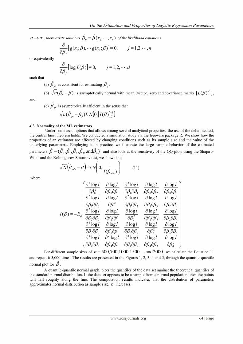
n , there exists solutions ),,(ˆ=ˆ1 nn xx of the likelihood equations.

njxgxg n

j

,1,2,=0,=);(),;( 1

or equivalently

djLj

,1,2,=0,=)(log

such that

(a) jn̂ is consistent for estimating j .

(b) )ˆ( nn is asymptotically normal with mean (vector) zero and covariance matrix ])([ 1L ,

and

(c) jn̂ is asymptotically efficient in the sense that

1)(0,)ˆ(

jjjjn INLn

4.3 Normality of the ML estimators

Under some assumptions that allows among several analytical properties, the use of the delta method,

the central limit theorem holds. We conducted a simulation study via the freeware package R. We show how the properties of an estimator are affected by changing conditions such as its sample size and the value of the

underlying parameters. Employing it in practice, we illustrate the large sample behavior of the estimated

parameters )ˆand,ˆ,ˆ,ˆ,ˆ(=ˆ43210 and also look at the sensitivity of the QQ-plots using the Shapiro-

Wilks and the Kolmogorov-Smornov test, we show that;

)(

10,ˆ

mle

mleI

NN

(11)

where

2

43424

2

14

2

04

243

2

3231303

24232

2

21202

2413121

2

2

101

2102010

2

10

2

0

2

logloglogloglog

logloglogloglog

logloglogloglog

logloglogloglog

logloglogloglog

=)(

lllll

lllll

lllll

lllll

lllll

EI

For different sample sizes of 2000and,150000,500,700,10=n , we calculate the Equation 11

and repeat it 5,000 times. The results are presented in the Figures 1, 2, 3, 4 and 5, through the quantile-quantile

normal plot for ̂ .

A quantile-quantile normal graph, plots the quantiles of the data set against the theoretical quantiles of the standard normal distribution. If the data set appears to be a sample from a normal population, then the points

will fall roughly along the line. The computation results indicates that the distribution of parameters

approximates normal distribution as sample size, n increases.



Figure 2: Monte Carlo Simulation of finite sample behaviour for normality of the parameter 0̂

Table 2: Test for Nomality 0

Kolmogorov-Smirnov test Shapiro-Wilks test

Sample size(n) Test

statistic (D)

P-value Test

statistic (D)

P-value

500 0.0501 0.09864 0.9948 0.0016

700 0.0664 0.0100 0.9961 0.0119

1000 0.0389 0.3246 0.9964 0.01997

1500 0.0325 0.5600 0.9987 0.3417

2000 0.0323 0.5567 0.9986 0.0462


Table 3: Test for Nomality Kolmogorov-Smirnov test Shapiro-Wilks test

Sample size(n) Test

statistic (D) P-value

Test

statistic (D) P-value

500 0.0600 0.0015 0.0600 0.0015

700 0.0584 0.0037 0.0654 0.0004

1000 0.0493 0.0156 0.0493 0.0156

1500 0.0431 0.0491 0.0431 0.0491

2000 0.0312 0.2846 0.0312 0.2846





Sample size(n) Test

statistic (D)

P-value

Test

statistic (D)

P-value

500 0.0309 0.2948 0.9998 0.0899

700 0.0346 0.1831 0.9970 0.1934

1000 0.0326 0.2378 0.9961 0.05678

1500 0.0295 0.3457 0.9974 0.0403

2000 0.0291 0.3661 0.9995 0.1101





Sample size(n) Test

statistic (D)

P-value Test

statistic (D)

P-value

500 0.0315 0.2731 0.9930 0.0001

700 0.0287 0.3825 0.9952 0.0029

1000 0.0167 0.5498 0.9969 0.0471

1500 0.0122 0.8700 0.9945 0.0707

2000 0.0096 0.8374 0.9988 0.7674



Sample size(n) Test

statistic (D)

P-value Test

statistic (D)

P-value

500 0.0426 0.0529 0.9958 0.0084

700 0.0363 0.1431 0.9916 .01843

1000 0.0459 0.2952 0.9968 .04791

1500 0.0225 0.6946 0.9973 0.09807

2000 0.0187 0.9001 0.9995 0.9980

V. Conclusion The study shows that the asymptotic properies of the maximum likelihood estimates of the logistic

regression model can be obtained by some transformation of the regularity conditions of the linear regression model. The simulation studies done show that there is consistency in the parameter estimates, where fixed

values of regression parameters are used, this shows that simulated estimates converge well to the fixed values

as the sample size approaches infinity. The finite behaviour of consistency is upheld.

On the otherhand, simulated result on the normality were taken using the Q-Q-plots and using the the

Kolmogorov-Smirnov and Shapiro-Wilks test. The analysis shows that the parameters are normally distributed,

this can be checked on the decrease of the statistic values on both tests and also from tables 1, 2, 3, 4 and 5, we

see that we fail to reject the null hypothesis at 5%= as the sample size increases and conclude that the

samples are taken from the normal distribution.

References [1] T. Amemiya. Advanced Econometric. Havard University Press, Cambridge, 1985.

[2] M. Beer. Asymptotic properies of the maximum likelihood estimator in [1] dichotomodi logistic regression model. 2001.

[3] David Collett. Modelling Binary Data. Chapman & Hall/CRC, New York, USA, second edition, (2002).

[4] Jerome Cornfield. Joint dependence of risk of coronary heart disease on serum cholesterol and systolic blood pressure: A

discriminant function analysis. In Federation Proceedings, volume 21, page 58, 1962.

[5] D. R. Sir Cox and E. J. Snell. Analysis of Binary Data. London.Chapman & Hall, 1989.

[6] J. S. Cramer. Logit Models from Economics and Other Fields. Cambridge University Press, 2003.

[7] K. S. Crump, H. A. Guess, and K. I. Deal. Confidence intervals and test of hypothesis concerning dose response relations inferense.

1977.



[8] R. C. Deutsch. Phd thesis. 2007.

[9] I. Fahrmeir and H. Kaufmann. Consistency and asymptotic normality of maximum likelihood estimator in generalized linear

models. 1985.

[10] J. Fan, M. Farmen, and J. Gijbels. Local maximum likelihood estimator and inference. 1998.

[11] C. Gourienx and A. Monfort. Asymptotic properties of the maximum likelihood estimation in dichotomous logit models. Journal

of Econometric 17, 83–97, 1981.

[12] H. A. Guess and K. S. Crump. Maximum likelihood estimation of dose response models subject absolutely monotonic constraints.

1978.

[13] D. W Hosmer and S. Lemeshow. Applied Logistic Regression. New York, Wiley, 1989.

[14] Trina Hosmer, David Hosmer, and Lloyd Fisher. A comparison of the maximum likelihood and discriminant function estimators of

the coefficients of the logistic regression model for mixed continuous and discrete variables. Communications in Statistics-

Simulation and Computation, 12(1):23–43, 1983.

[15] D. N. Joanes. Reject inference applied to logistic regression for credit scoring. 1993.

[16] G.S Maddala. Limited dependent variables and quantitative variables. 1983.

[17] P. McCullagh and J. A. Nelder. Generalized linear models. 1989.

[18] L. McFadden. Conditional logit analysis of qualitative choice behaviour. 1974.

[19] L. Nordberg. Asymptotic normality of maximum likelihood estimators based on independent unequal distributed observations in

exponential family models. 1980.

[20] Leandro Pardo. Statistical inference based on divergence measures. CRC Press, 2005.

[21] R. Pastor-Barriuso, E. Guallar, and J. Coresh. Use of two-segmented logistic regression to estimate change of point in

epidemological studies. 1998.

[22] R. Pastor-Barriuso and E. Guallar. Transition model for change point estimation on logistic regression. 2003.

[23] M. Rashid and N. Shifa. Consistency of the maximum likelihood estimator in logistic regression model:a different approach. 2009.

[24] R.Christensen. Log-Linear Models and Logistic Regression. Springer-Verlag Inc., New York, USA, 1997.

[25] J Wilde. A note on gmm estimator of probit models with endogenous regression . 2008.

on the estimation and properties of logistic regression ... · pdf fileon the estimation and...

Documents