Noname manuscript No.(will be inserted by the editor)

On the enumerative natureof Gomory’s dual cutting plane method

Egon Balas · Matteo Fischetti · Arrigo

Zanette

Received: 30 April 2009, rev. December 14, 2009 / Accepted: date

Abstract For thirty years after their invention half a century ago, cutting planes for

integer programs have been an object of theoretical investigations that had no apparent

practical use. When they finally proved their practical usefulness in the late eighties,

that happened in the framework of branch and bound procedures, as an auxiliary

tool meant to reduce the number of enumerated nodes. To this day, pure cutting

plane methods alone have poor convergence properties and are typically not used in

practice. Our reason for studying them is our belief that these negative properties

can be understood and thus remedied only based on a thorough investigation of such

procedures in their pure form.

In this paper, the second in a sequence, we address some important issues arising

when designing a computationally sound pure cutting plane method. We analyze the

dual cutting plane procedure proposed by Gomory in 1958, which is the first (and most

famous) convergent cutting plane method for integer linear programming. We focus on

the enumerative nature of this method as evidenced by the relative computational suc-

cess of its lexicographic version (as documented in our previous paper on the subject),

and we propose new versions of Gomory’s cutting plane procedure with an improved

performance. In particular, the new versions are based on enumerative schemes that

treat the objective function implicitly, and redefine the lexicographic order on the fly

to mimic a sound branching strategy. Preliminary computational results are reported.

Keywords Cutting Plane Methods · Gomory Cuts · Degeneracy in Linear Program-

ming · Lexicographic Dual Simplex · Computational Analysis

E. BalasCarnegie Mellon University, Pittsburgh, PAE-mail: eb17@andrew.cmu.edu

M. FischettiDEI, University of PadovaE-mail: matteo.fischetti@unipd.it

A. ZanetteDEI, University of PadovaE-mail: zanettea@gmail.com

2

1 Introduction

Let us consider the following Integer Linear Program (ILP):

min cT x

Ax = b

x ≥ 0 integer

where A ∈ Zm×n, b ∈ Zm, and c ∈ Zn. Let P := {x ∈ <n : Ax = b, x ≥ 0} denote the

LP relaxation polyhedron, that we assume to be bounded.

The structure of a pure cutting plane algorithm for the solution of an ILP problem

can be outlined roughly as follows:

1. solve the LP relaxation min{cT x : x ∈ P} and denote by x∗ an optimal vertex

2. if x∗ is integer, we are done

3. otherwise, search for a violated cut, i.e., an inequality αT x ≤ α0 whose associated

hyperplane separates x∗ from the convex hull of integer feasible points, introduce a

slack variable to bring the cut to its equality form, add it to the original formulation,

and repeat.

Cut generation is a crucial step in the above method. In 1958, Gomory [11] (see

also [13]) proposed an elegant procedure to generate violated cuts, showing that x∗

can always be separated by means of a cut easily derived from a row of the optimal LP

tableau. This cut, expressing the requirement that the sum of fractional parts of the

coefficients must be at least equal to the fractional part of the righthand side, can be

deduced by the following simple rounding argument: Given any equation∑nj=1 γjxj =

γ0 valid for P , the fact that x is constrained to be nonnegative and integer implies that

both∑nj=1bγjcxj ≤ bγ0c and

∑nj=1dγjexj ≥ dγ0e are valid inequalities. Subtracting

the above equation from either of these inequalities yields a valid cut expressing the

requirement concerning the sum of fractional parts.In order to find a violated cut,

Gomory’s proposal is to apply the above procedure to the equation associated with

a row of the LP optimal tableau whose basic variable is fractional: we will refer to

this row as the cut generating row, and to the corresponding basic variable as the cut

generating variable.

The resulting cuts are called Gomory Fractional Cuts (GFCs) and can be used to

derive a finitely-convergent cutting plane method. GFCs are also known as Chvatal-

Gomory (CG) cuts after the work of Chvatal [7] who proved some basic polyhedral

properties of these cuts. It is interesting to observe that the connection between GFCs

(in their equivalent “fractional form” originally described by Gomory) and CG cuts

(in the all-integer form introduced above) was not recognized immediately. In our view

this is not surprising since, as we will discuss in the sequel, the specific GFCs actually

used in Gomory’s method are based on enumerative (rather than purely polyhedral)

considerations.

In 1960, Gomory [12] introduced the Gomory Mixed Integer (GMI) cuts to deal

with the mixed-integer case. In case of pure ILPs, GMI cuts are applicable as well,

and actually dominate GFCs in that each variable xj always receives a coefficient

increased by a quantity θj ∈ [0, 1) with respect to the GFCs (writing the GMI in its

≤ form, with the same right-hand-side value as in its GFC counterpart). So, from a

strictly polyhedral point of view, there is no apparent reason to insist on GFCs when

a stronger replacement is readily available at no extra computational effort. However,

3

the coefficient integrality of GMI cuts is no longer guaranteed, and some nice numerical

properties of GFCs are lost. In addition, GMI cuts introduce continuous slack variables

that may receive weak coefficients in the next iterations, leading to weaker and weaker

GMI cuts in the long run. As a result, it is unclear whether GFCs or GMI cuts are

better suited for a cutting plane method for pure integer programs based on tableau

cuts.

We face here a fundamental issue in the design of pure cutting plane methods based

on Gomory’s (mixed-integer or fractional) cuts read from the LP optimal tableau.

Because we expect to generate a long sequence of cuts that eventually lead to an

optimal integer solution, we have to take into account side effects of the cuts that

are unimportant when just a few cuts are used (within an enumeration scheme) to

improve the LP bound. It is important to stress that the requirement of reading the

cuts directly from the optimal LP tableau makes the Gomory method intrinsically

different from a method that works solely with the original polyhedron where the cut

separation is decoupled from the LP reoptimization, as in the recent work of Fischetti

and Lodi [10] on CG cuts, or Balas and Saxena [3] and Dash, Gunluk and Lodi [9] on

GMI (split/MIR) cuts.

In Zanette, Fischetti and Balas [17] we implemented the lexicographic version of

the Gomory method that is actually used in one of the two finite convergence proofs

given in [13]. Gomory himself never advocated the practical use of this method; on

the contrary, he stressed that its sole purpose was to provide one of the two finiteness

proofs, and that in practice other choice criteria in the pivoting sequence were likely

to work better. (Actually, we have no information on anybody ever having tried exten-

sively this method before.) In computational testing on a battery of MIPLIB problems

we compared the performance of the lexicographic variant with that of the “textbook”

Gomory algorithm, both in the single-cut and in the multi-cut (rounds of cuts) ver-

sion, and showed that it provides a radical improvement over the standard procedure.

In particular, we reported the exact solution of ILP instances from MIPLIB such as

stein15, stein27, and bm23, for which the textbook Gomory cutting plane algorithm

is not able to close more than a tiny fraction of the integrality gap.

In the present paper we analyze in more detail the characteristics that make the lex-

icographic Gomory method substantially better than its textbook (nonlexicographic)

counterpart, with the help of a number of illustrative examples. In particular, in Sec-

tion 2 we discuss the role of dual degeneracy in pure cutting plane methods, and address

the lexicographic dual simplex method. In Section 3, the relationship between GFCs

and the sign pattern of lex-optimal tableaux is addressed, whereas in Section 4 the

enumerative nature of Gomory method is discussed. Section 5 introduces some vari-

ants of the Gomory method where the objective function is treated implicitly. Section 6

describes a Gomory-like method where the lexicographic order is redefined on the fly

to mimic a sound branching strategy. Preliminary computational results are reported

Section 7. Some conclusions are finally drawn in Section 8.

2 Dual degeneracy and the lexicographic dual simplex

Dual degeneracy arises in an LP when alternative optimal vertices exist. Dual degener-

acy occurs almost invariably when solving ILPs by means of cutting plane algorithms.

This is due to the fact that cutting plane methods introduce a large number of cuts that

tend to become almost parallel to the objective function, whose main goal is to prove

4

or to disprove the existence of an integer point with a certain value of the objective

function. In this way, it is the cutting plane method itself that injects dual degeneracy

into the LPs to be solved. As a consequence, every sound pure cutting plane method

has to deal with it.

It is worth observing that dual degeneracy is an intrinsic property of the LPs en-

countered when solving an NP-hard problem by pure cutting plane methods, even if

the original LP is not dual degenerate. Indeed, if one could sensibly assume that all the

LPs to be solved during the cutting plane process were not dual degenerate, then the

following naive ILP method would work in pseudo-polynomial time. At each iteration,

let x∗ be the (unique) optimal LP vertex and consider its associated optimal tableau.

If cT x∗ is fractional, then add the cut cT x ≥ dcT x∗e (which is just a weakening of the

GFC that can be read from the tableau row associated with the objective function).

Otherwise, add any cut (e.g.,∑j∈N xj ≥ 1 where N is the index set of the nonbasic

variables) and observe that, due the dual nondegeneracy assumption, the LP optimal

value cannot stay unchanged after reoptimization. It then follows that, after the addi-

tion of at most two cuts (the first to change x∗, and the second to move the objective

function), the optimal LP value increases by, at least, one unit. Thus the above method

reaches the optimal ILP value in a pseudo-polynomial number of steps, and then ex-

hibits (again, because of the nondegeneracy assumption) a unique LP solution that is

integer.

In one of his two proofs of convergence, Gomory used the lexicographic dual simplex

to cope with degeneracy. The lexicographic dual simplex is a generalized version of

the simplex algorithm where, instead of considering the minimization of the objective

function, viewed without loss of generality as an additional integer variable x0 = cT x,

one is interested in the minimization of the entire solution vector (x0, x1, . . . , xn), where

(x0, x1, . . . , xn) <LEX (y0, y1, . . . , yn) means that there exists an index k such that

xi = yi for all i = 1, . . . , k − 1, and xk < yk.

In the lexicographic, as opposed to the usual, dual simplex method the ratio test

is modified so as to involve not just two scalars (reduced cost and pivot candidate),

but an entire tableau column and a scalar; see e.g. [14]. So, its implementation is

straightforward, at least in theory. In practice, however, there are a number of major

concerns that limit the applicability of this approach:

1. the ratio test may be quite time consuming;

2. the ratio test may fail in selecting the right column to preserve lex-optimality, due

to round-off errors;

3. the algorithm rigidly prescribes the pivot choice, which excludes the possibility of

applying much more effective pivot-selection criteria.

The last point is maybe the most important. As a practical approach should not

interfere too much with the black-box LP solver used, one could think of using a

perturbed linear objective function x0 + ε1x1 + ε2x2 . . .+ εnxn, where x0 is the actual

objective and 1� ε1 � ε2 � . . .� εn are suitable weights. This approach is however

numerically unacceptable. We proposed in [17] the following alternative method, akin

to the slack fixing used in the sequential solution of preemptive linear goal programs

[2,16]; see also Balinski and Tucker [4].

Starting from an optimal solution (x∗0, x∗1, . . . , x

∗n) with respect to x0 only, we want

to find another basic solution for which x0 = x∗0 but x1 < x∗1 (if any), by exploiting

dual degeneracy. So, we fix the variables that are nonbasic (at their bound) and have a

nonzero reduced cost. This implies the fixing of the objective function value to x∗0, but

5

x0 x1 x3 x5 x4 x2 x11 x10 x9 x8 x6 x7

x0 = x∗0 1 0 0 0 0 0 0 0 0 0 – –

x1 = x∗1 0 1 0 0 0 0 0 0 – – * *

x3 = x∗3 0 0 1 0 0 0 0 – * * * *

x5 = x∗5 0 0 0 1 – – – * * * * *

Fig. 1 Sign pattern in a lexicographic optimal tableau

has a major advantage: since we fix only variables at their bounds, the fixed variables

will remain out of the basis in all the subsequent steps. Then we reoptimize the LP

in the free variables (i.e. those with zero reduced cost) by using x1 as the objective

function to be minimized, fix other nonbasic variables, and repeat. The method then

keeps optimizing subsequent variables, in lexicographic order, thus iteratively reducing

the extent of dual degeneracy either no degeneracy remains, or all variables are fixed. At

this point we can keep the current (lex-optimal) basis and unfix all the fixed variables.

This approach proved to be quite effective and stable in practice: even for large

problems, where the classical algorithm is painfully slow or even fails, our alterna-

tive method requires a reasonable computing time to convert the optimal basis into a

lexicographically-minimal one.

3 Lexicographic dual simplex and Gomory cuts

GFCs and the dual lexicographic simplex are intimately related to each other, in the

sense that GFCs are precisely the kind of cuts that allow for a significant lexicographic

improvement of the solution found after each reoptimization. It is therefore not sur-

prising that Gomory’s (first) proof of convergence relies on the use of the lexicographic

dual simplex [13]. We next outline the main ingredients of this proof, in a slightly

modified form that makes it more suitable for implementation.

In what follows we assume without loss of generality that the tableau rows have

been sorted in increasing order of the corresponding basic variables. The lexicographic

dual simplex method starts with a lexicographically optimal tableau, which means that

all columns are lexicographically positive or lexicographically negative—depending on

whether one minimizes or maximizes, and on the sign rule one follows in representing

the columns. To fix our ideas, let us opt for minimization and the sign rule that requires

all columns to be lexicographically negative, which means that the first column entry

is the negative of what usually goes under the name of reduced cost. Thus the first

nonzero entry of each nonbasic column is negative.

Example 1. Let us consider the lexicographic optimal tableau of Figure 1, where the

entry in row i associated with variable xj will be denoted by aij . The rows have

been sorted in increasing order of the corresponding basic variables, and the objective

function variable x0 (with its sign) is basic in the first row (row 0). The tableau columns

have been rearranged for typographical reasons. Note that the low-index variables x2

and x4 are nonbasic, so x∗2 = x∗4 = 0, whereas x∗1, x∗3, x∗5 ≥ 0. Entries marked by a minus

sign are strictly negative, whereas those marked by an asterisk are non restricted in

sign.

6

As claimed, the first nonzero entry in each nonbasic column is negative, a property

that guarantees that x∗ is a lexicographic optimal solution. Indeed, take any feasible

solution x that is lexicographically not worse than x∗. We will prove that x = x∗, which

implies that no strictly better solution than x∗ exist. The equation associated with the

first row reads x0 + a0,6x6 + a0,7x7 = x∗0, which implies x0 ≥ x∗0 for all x ≥ 0 due

to sign assumption a0,6, a0,7 < 0. Since every solution with x6 + x7 > 0 has a strictly

worse value for x0, we can fix the nonbasic variables x6 = x7 = 0 and analyze x1. From

the equation in the second row we have x1 +a1,9x9 +a1,8x8 = x∗1, i.e., x1 ≥ x∗1 because

a1,9, a1,8 < 0. As before, we can fix the nonbasic variables x9 = x8 = 0 and proceed

with the analysis of the next variable in the lexicographic order, x2. This is itself a

nonbasic variable that cannot be decreased, so we fix x2 = 0 and proceed with the

analysis of the remaining variables, in their lexicographic order x3, x4, · · · , x11, each

time fixing to zero some nonbasic variables. In the end, all nonbasic variables are fixed

to zero, and the only remaining feasible choice is x = x∗, as required.

The above example also suggests that an optimal tableau with the required sign

pattern (and hence lexicographically optimal) can always be obtained through a se-

quence of reoptimizations on a smaller and smaller set of variables, each bringing a

tableau row (viewed as an objective function) to its “reduced cost form” with non-

positive entries for all nonbasic (nonfixed) variables—which is precisely the way we

compute it.

�

The tableau sign pattern has a fundamental role in Gomory’s method in that it

guarantees a certain property of the sequence of cuts generated under the lexicographic

rule, provided that the “right” rounding operation is used in generating the cuts. As a

matter of fact, the Gomory method using the lexicographic simplex can be proved to be

convergent only in case the kind of rounding used is consistent with the lexicographic

objective. We next briefly discuss the GFC properties that lead to a convergent method.

Let the ith row of the current tableau be

xh +∑j∈J−

aijxj +∑j∈J+

aijxj = ai0 (= x∗h)

where xh is the basic variable in row i, J− is the set of indices of nonbasic variables

such that aij ≤ 0, and J+ is the set of indices of nonbasic variables such that aij > 0.

Moreover, let us suppose h is the first index such that x∗h is fractional.

A key observation is that, due to the lexicographic sign pattern, for each j ∈ J+

there exists a row t < i with atj < 0; see, e.g., Figure 1.

The rounding procedure can be used to obtain the following GFC, in integer form:

xh +∑j∈J−

daijexj +∑j∈J+

daijexj ≥ dx∗he (1)

Note that we round the coefficients of the original row upward. The choice is mo-

tivated by the fact that, for a minimization problem, we expect to lexicographically

minimize the solution vector of the linear relaxation, hence the cut is intended to

contribute in the opposite direction, namely, to increase lexicographically the solution

vector.

7

Clearly, the round-up operation maintains the nonpositiveness of the coefficients in

J− and the positiveness of those in J+. In case no xj with j ∈ J+ becomes strictly

positive after the lexicographic reoptimization, cut (1) requires

xh ≥ dai0e −∑j∈J−

daijexj ≥ dx∗he.

Otherwise, due to the particular tableau sign pattern, the increase of some xj with

j ∈ J+ implies the increase of some higher lex-ranked basic variable xr by a positive

amount.

In both cases, a significant lexicographic step is performed: either the cut-generating

variable xh jumps, at least, to its upper integer value dx∗he, or some higher lex-ranked

variable increases by a positive amount. This guarantees a substantial increase of the

lexicographic value of the current LP solution x∗, a property that implies convergence

after a finite number of steps; see [13] for more details.

Example 1 (cont.d). Take again Example 1 of Figure 1, and assume that the first

fractional variable is x∗5, so the GFC is read from the last tableau row (row 3). In this

case, J− ⊇ {4, 2, 11} and J+ ⊆ {10, 9, 8, 6, 7} and the “right” GFC reads

x5+da3,10ex10+da3,9ex9+da3,8ex8+da3,6ex6+da3,7ex7 ≥ dx∗5e−da3,4ex4−da3,2ex2−da3,11ex11

For any feasible LP solution x that satisfies the equation above, one of the following

cases apply:

– If x6 + x7 > 0, then from tableau row 0 we have x0 > x∗0.

– If x6 = x7 = 0 but x9 + x8 > 0, then x0 = x∗0 and, from tableau row 1, we have

x1 > x∗1.

– If x6 = x7 = x9 = x8 = 0 but x10 > 0, then x0 = x∗0, x1 = x∗1, x2 ≥ x∗2 = 0 while

tableau row 2 implies x3 > x∗3.

– If x6 = x7 = x9 = x8 = x10 = 0, the GFC implies x5 ≥ dx∗5e−da3,4ex4−da3,2ex2−da3,11ex11 ≥ dx∗5e because a3,4, a3,2, a3,11 < 0.

�

Figure 2 illustrates on a small instance the contrast between the behavior of the

textbook version and the lexicographic one of Gomory’s cutting plane algorithm: In

the textbook version, a week bound obtained after adding a few cuts cannot be further

improved, whereas in the lexicographic one a substantially higher bound is obtained.

Moreover, in the lexicographic version the cut coefficients remain throughout the run

in the low digits, whereas in the textbook version they keep steadily growing (when

the cuts are expressed in the structural variables, hence with integer coefficients).

This bad behavior would however be prevented by reading GFCs from the lexico-

graphic optimal tableau, in that a very long sequence of iterations without a significant

change in one of the components of the LP solution could not occur. Actually, even

with the lexicographic method it may well be the case that only a small change of the

LP solution occurs after the addition of a cut, but this implies that an integer-valued

variable of lower rank increases by a nonzero quantity. So, in the next iteration this

variable (or a lower-rank one) will generate a new GFC that will either increase its

8

0 20 40 605

6

7

8

9Bound

#itrs

obje

ctiv

e va

lue

LexTb

0 20 40 6010

0

105

1010

Cut coefficients

#itrsav

erag

e cu

t coe

ffici

ent

LexTb

Fig. 2 Lexicographic (Lex) vs. textbook (Tb) Gomory method; single-cut version on instancestein15 with an initial LP bound of 5 and integer optimum value 9.

value to its nearest integer, or it will increase another integer-valued variable with

lower rank. It then follows that, after at most n steps, a significant change in the LP

solution (or in its cost) must necessarily occur.

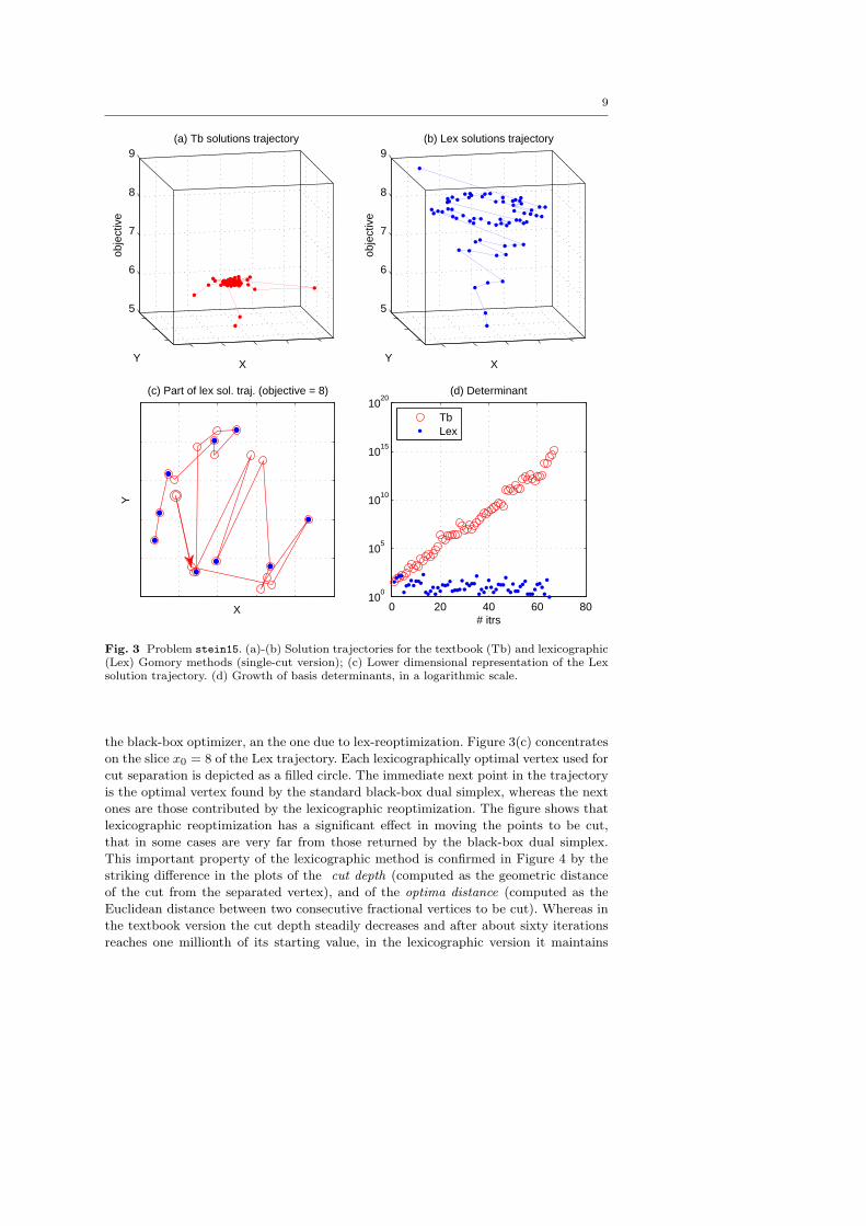
Figure 3, taken from [17], gives a representation of the trajectory of the LP optimal

vertices to be cut (along with a plot of the basis determinant) when the textbook and

the lexicographic methods are used, again for problem stein15. In Figures 3(a) and

(b), the vertical axis represents the objective function value. As to the XY space,

it is a projection of the original 15-dimensional variable space obtained by using a

multidimensional scaling procedure [6] that preserves the metric of the original 15-

dimensional space as much as possible. In particular, the original Euclidean distances

tend to be preserved, so points that look close one to each other in the figure are likely

to be also close in the original space.

Both Figures 3(a) and (b) show that the initial lower bound of value 5 is improved.

According to Figure 3(a), however, after a few iterations the textbook method reduces

to cutting points belonging to a shrunk region. This behavior is in a sense a consequence

of the efficiency of the underlying LP solver, that has no reason to change the LP

solution once it becomes optimal with respect to the original objective function—the

standard dual simplex will stop as soon as a feasible point (typically very close to the

previous optimal vertex) is reached. As new degenerate vertices are created by the cuts

themselves, the textbook method enters a feedback loop that is responsible for the

exponential growth of the determinant of the current basis, as reported in Figure 3(d).

On the contrary, as shown in Figure 3(b), the lexicographic method prevents this

drawback by always moving the fractional vertex to be cut as far as possible (in the

lexicographic sense) from the previous one. Note that, in principle, this property does

not guarantee that there will be no numerical problemsdue to huge determinants, but

the method seems to work pretty well in practice.

Figure 3(c) offers a closer look at the effect of lexicographic reoptimization. Recall

that our implementation of the lexicographic dual simplex method involves a sequence

of reoptimizations, each of which produces an alternative optimal vertex possibly dif-

ferent from the previous one. As a result, between two consecutive cuts our method

internally traces a trajectory of equivalent solutions, hence one can distinguish between

two contributions to the movement of x∗ after the addition of a new cut: the one due to

9

5

6

7

8

9

X

(a) Tb solutions trajectory

Y

obje

ctiv

e

5

6

7

8

9

X

(b) Lex solutions trajectory

Yob

ject

ive

X

Y

(c) Part of lex sol. traj. (objective = 8)

0 20 40 60 8010

0

105

1010

1015

1020

# itrs

(d) Determinant

TbLex

Fig. 3 Problem stein15. (a)-(b) Solution trajectories for the textbook (Tb) and lexicographic(Lex) Gomory methods (single-cut version); (c) Lower dimensional representation of the Lexsolution trajectory. (d) Growth of basis determinants, in a logarithmic scale.

the black-box optimizer, an the one due to lex-reoptimization. Figure 3(c) concentrates

on the slice x0 = 8 of the Lex trajectory. Each lexicographically optimal vertex used for

cut separation is depicted as a filled circle. The immediate next point in the trajectory

is the optimal vertex found by the standard black-box dual simplex, whereas the next

ones are those contributed by the lexicographic reoptimization. The figure shows that

lexicographic reoptimization has a significant effect in moving the points to be cut,

that in some cases are very far from those returned by the black-box dual simplex.

This important property of the lexicographic method is confirmed in Figure 4 by the

striking difference in the plots of the cut depth (computed as the geometric distance

of the cut from the separated vertex), and of the optima distance (computed as the

Euclidean distance between two consecutive fractional vertices to be cut). Whereas in

the textbook version the cut depth steadily decreases and after about sixty iterations

reaches one millionth of its starting value, in the lexicographic version it maintains

10

0 20 40 6010

−6

10−4

10−2

100

cut d

epth

Tb

0 20 40 6010

−6

10−4

10−2

100

Lex

0 20 40 600

1

2

3

4

optim

a di

stan

ce

#itrs0 20 40 60

0

1

2

3

4

#itrs

Fig. 4 Cut depth and distance between consecutive fractional solutions for the textbook (left)and lexicographic (right) Gomory methods (single-cut version on instance stein15)

0 20 40 605

6

7

8

9Bound

#itrs

obje

ctiv

e va

lue

right directionwrong direction

0 20 40 6010

0

105

1010

Cut coefficients

#itrs

aver

age

cut c

oeffi

cien

t

right directionwrong direction

Fig. 5 Impact of rounding direction on GFCs read from the lex-optimal tableau rows (single-cut version on instance stein15)

throughout its original order of magnitude. Similarly, the distance between two con-

secutive solutions to be cut is orders of magnitude larger in the lexicographic version

than in the textbook one.

Finally, to show the importance of reading the “right” GFC from the tableau

rows, in Figure 5 we plot the behavior on stein15 of two variants of the lexicographic

method—in its single-cut version. One variant exploits the right (≥) GFCs, while the

11

other uses their wrong (≤) counterpart. The figure shows a huge difference not only in

terms of gap closed, but also of numerical stability (coefficient size).

4 Enumerative interpretation of the lexicographic cutting plane procedure

The Gomory algorithm coupled with lexicographic reoptimizations has a nice interpre-

tation in terms of implicit enumeration, as observed first by Nourie and Venta [15]; see

also [14]. The underlying enumeration tree has, at level zero, the nodes corresponding

to the possible different integer values of the objective function variable (x0). Lower

levels correspond to the possible integer values of other variables, in lexicographic order

x1, x2, · · · Leaves correspond to integer solutions, ranked in increasing lexicographic

order. During the lexicographic Gomory method the tree is visited in a depth–first

manner. Once a fractional value is found, the separated GFC cut ensures either to

move the first fractional variable to its next integer value in a kind of branching step,

or to backtrack the search to an upper level of the tree.

Example 2. Consider the 0-1 ILP

min −4x1 − 8x2 + 4x3 +7

4x1 + 4x2 ≥ 4

4x2 ≤ 4

4x1 + 4x2 − 4x3 ≤ 3

x1, x2, x3 ∈ {0, 1}

The underlying search tree is depicted in Figure 6. In the figure, the horizontal

axis reports the possible values of the solution vector (x0, x1, x2, x3), in increasing

lexicographic order. For illustration purposes, the scale is obtained by considering a

function z =∑nj=0 ε

jxj for a sufficiently small ε > 0 that maps lex-increasing solution

vectors into increasing scalar values z. In our case, ε = 0.2 suffices. For typographical

reasons, the z scale is interrupted at some points.

The optimal solution of the LP relaxation has value 0, and the corresponding lexi-

cographic optimal tableau (with the sign convention used in Figure 1) is as follows; note

that the nonbasic variable x2 at its upper bound has been replaced by its complement.

x0 x1 1−x2 x3 s1 s2 s3

x0 = 0 1 0 -4 0 0 0 -1

x1 = 0 0 1 -1 0 -0.25 0 0

x3 = 0.25 0 0 0 1 -0.25 0 -0.25

s2 = 0 0 0 -4 0 0 1 0

The Gomory method with lexicographic reoptimizations then produces the follow-

ing sequence of lex-optimal LP solutions, that is also plotted in Figure 6.

12

zo o o o o o o o o o o o o o o o

x0

x1

x2

x3

0.042 0.12 0.406 1.044 1.148 1.781

Fig. 6 The enumeration implicitly performed by the “right” Gomory method (with lexico-graphic reoptimization and GFCs in ≥ form)

z x0 x1 x2 x3 # pivots

0.042 0 0 1 0.25 2

0.120 0 0.375 1 0.625 1

0.406 0.2 0.8 0.95 1 1

1.044 1 0 1 0.5 1

1.148 1 0.5 1 1 1

1.781 1.667 0.333 1 1 1

3.048 3 0 1 1 1

As expected, the sequence is monotonically increasing in lexicographic sense (and

also in terms of z), and each GFC moves the fractional point by a significant quantity

that can be interpreted in terms of branching/backtracking along the tree. For example,

a branching occurs at step 2 (z = 0.406) when x∗0 = 0.2 is moved to 1, whereas a

backtracking arises at step 4 (z = 1.148) when the subtree x0 = 1, x1 = 1 is not

explored.

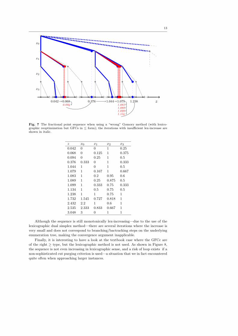
If the lexicographic method is still used but the “wrong” GFCs are used, instead,

the following sequence of LP solutions is traced; see Figure 7 for an illustration.

13

zo o o o o o o o o o o o o o o o

x0

x1

x2

x3

0.042 0.0680.094

0.376 1.044 1.0791.0831.0891.0991.134

1.238

Fig. 7 The fractional point sequence when using a “wrong” Gomory method (with lexico-graphic reoptimization but GFCs in ≤ form); the iterations with insufficient lex-increase areshown in italic.

z x0 x1 x2 x3

0.042 0 0 1 0.25

0.068 0 0.125 1 0.375

0.094 0 0.25 1 0.5

0.376 0.333 0 1 0.333

1.044 1 0 1 0.5

1.079 1 0.167 1 0.667

1.083 1 0.2 0.95 0.6

1.089 1 0.25 0.875 0.5

1.099 1 0.333 0.75 0.333

1.134 1 0.5 0.75 0.5

1.238 1 1 0.75 1

1.732 1.545 0.727 0.818 1

2.432 2.2 1 0.6 1

2.535 2.333 0.833 0.667 1

3.048 3 0 1 1

Although the sequence is still monotonically lex-increasing—due to the use of the

lexicographic dual simplex method—there are several iterations where the increase is

very small and does not correspond to branching/bactracking steps on the underlying

enumeration tree, making the convergence argument inapplicable.

Finally, it is interesting to have a look at the textbook case where the GFCc are

of the right ≥ type, but the lexicographic method is not used. As shown in Figure 8,

the sequence is not even increasing in lexicographic sense, and a risk of loop exists if a

non-sophisticated cut purging criterion is used—a situation that we in fact encountered

quite often when approaching larger instances.

14

zo o o o o o o o o o o o o o o o

x0

x1

x2

x3

0.042 0.12 0.406 1.148 1.238 1.7811.845

1.901

Fig. 8 The fractional point sequence when using a “textbook” Gomory method without lex-icographic reoptimization.

�

5 Getting rid of the objective function

In order to better exhibit the enumerative nature of Gomory lexicographic cutting

plane procedure, we will compare it to a specialized Branch&Bound (B&B) scheme

constructed for this purpose, which we call lexicographic branch-and-bound. Such a

comparison permits us to make some provable statements about the efficiency of the

lexicographic cutting plane procedure when compared to a similar purely enumerative

one.

For this purpose, one has to modify the Gomory method because it considers the

objective function as a general-integer variable x0 associated with the very first level

of the tree. On the contrary, B&B algorithms treat the objective function differently

from the other variables, using it only for fathoming purposes. This is a wise operation

in that it typically reduces the size of the overall search tree and isolates a linear

expression (the objective function) whose coefficients often differ substantially from

those of other constraints.

Example 3. Drawbacks deriving from the use of the objective function as the lexico-

graphically most-significant variable can be illustrated with the help of the following

small example, which is the 0-1 version of a famous pathological case due to Cook,

Kannan and Schrijver [8]; see also Nemhauser and Wolsey [14] (p. 382, ex. 12):

max{y : x1 + x2 + y ≤ 2, y ≤ x1, y ≤ x2, x1, x2 ∈ {0, 1}, y ≥ 0}

15

· · · · · ·

−z

x1

x2

−z =x1 =x2 =

−666.6670.6670.667

−666.000

0.6660.666

−665.6690.6690.669

−665.000

0.6650.665

−664.6710.6710.671

500.0

0.50.5

500.01.00.5

−499.7500.7500.750

−499.000

0.4990.499

−499.0001.0000.499

−498.7510.7510.751

−0.9990.9990.999

0

00

Fig. 9 Tree implicitly explored by the lexicographic Gomory method on a small example.

In the original example, y is a continuous variable, which makes the standard Gomory

cutting plane method using GMIs nonconvergent. By replacing the continuous variable

y by y = z/M , z ≥ 0 and integer (for a large integer M > 0 so as to simulate

very small fractionalities for y) we obtain a pure ILP instance that requires about

M GFCs to be solved by the lexicographic Gomory method. Figure 9 illustrates the

tree implicitly explored by the lexicographic Gomory cutting plane algorithm when

M = 1000, i.e., when solving min{−z : z+1000x1 +1000x2 ≤ 2000, z ≤ 1000x1, z ≤1000x2, x1, x2 ∈ {0, 1}, z ∈ Z+}. Levels from the root correspond to variables −z, x1,

and x2, respectively. The solution values are reported below the pictorial representation

of the tree, aligned on two different layers representing two different types of elementary

steps. For each layer, solution values are reported between square brackets. Note the

large number of integer objective function values that need to be enumerated. The

same instance can however be solved with just a pair of GFCs if one gets rid of the

problematic variable z by using the modified cutting plane scheme to be described

next.

�

To better mimic the B&B approach, we remove the objective function and replace

it with a constraint that uses the current incumbent integer value U . In this modified

approach, the lexicographic Gomory cutting plane method is used, without objective

function, as a feasibility subroutine to find an integer solution of the original problem

amended by the (invalid) upper bound constraint cT x ≤ U − 11. If an integer solution

is found, the incumbent solution and its value U are updated, and the cutting-plane

subroutine is called again. The process stops when the cutting plane subroutine certifies

the infeasibility of the current subproblem.

To illustrate the modified Gomory algorithm above, that we call the Lexicographic

Cutting Plane method (L-CP), let us concentrate on a 0-1 ILP and compare it with

the following Lexicographic B&B procedure (L-B&B).

1 For technical reasons, the upper bound constraint is written as 2cT x ≤ 2U − 1 so as toavoid to have it tight when an integer solution is found.

16

L-B&B differs from straightforward lexicographic enumeration (in increasing order)

in that it uses the LP relaxation to generate bounds and prune the search tree. The

complete lexicographic tree is a binary tree whose leaves represent all 0-1 n-vectors in

lexicographically increasing order from left to right. In this tree, each node has one

parent and two children: a left child joined to the parent by a left edge, and a right

child joined to the parent by a right edge. The tree has 2(n+1) − 1 nodes, of which 2n

leaves.

Procedure L-B&B is defined on a lexicographic search tree T , which is a subtree

of the complete tree pruned by the bounds generated by the LP solver. Each node on

level p of T is associated with a 0-1 p-vector representing the first p components of

some x ∈ {0, 1}n. In particular, with every n-vector x with components 0 ≤ xj ≤ 1,

we associate a node N(x) of T as follows: if xi is the first fractional component of x,

then N(x) = (x1, . . . , xi−1), i.e., N(x) is the node on level i − 1 of T defined by the

first i− 1 components of x. L-B&B can now be described as follows.

Let the problem to be solved be min{cT x : x ∈ P ∩ Zn}, where the set of

linear constraints defining P contains the bound condition x ∈ [0, 1]n. We write the

lexicographic linear programming relaxation of this as

lex- min{0T x : x ∈ P, 2cT x ≤ 2U − 1} (LP)

where U is an upper bound on the optimal integer solution value.

1. Solve LP amended by the branching conditions associated with the current node. If

LP is infeasible, discard the current node and go to step 3 (backtrack). Otherwise,

let x∗ be the lex-optimal solution. If x∗ is integer, store it in place of the incumbent,

update U = cT x∗, and return to step 1.

2. Branch: Let x∗i be the first fractional component of x∗. Go to node N(x∗) of T , dis-

card the left child (x∗, . . . , x∗i−1, 0) of N(x∗), go to the right child (x∗, . . . , x∗i−1, 1)

of N(x∗), and apply step 1.

3. Backtrack: discard the current node and go to its parent. If the parent is reached

through a right arc, backtrack again. Otherwise go to the parent’s right child, and

apply step 1.

The procedure stops when the next step is to backtrack from the root node. The

last stored solution is optimal (if no such solution exist, then the problem is infeasible).

The correctness of L-B&B follows from the following facts: If LP is infeasible, then

no descendent of the current node can have a feasible solution. If x∗ is a lexico-minimal

solution to the LP relaxation of the current subproblem, then any integer solution that

shares the first i − 1 components of x∗ is among the descendants of the node N(x∗),and the left child of N(x∗) can be discarded as lexicographically smaller than x∗ (the

left child has xi = 0 versus 0 < x∗i < 1).

The number of steps required by L-B&B is of course O(2n), the number of leaves

of the complete enumeration tree. The actual number can be much smaller, and it

depends on how tightly the problem is constrained and what lexicographic ordering

one chooses.

It is not difficult to show that L-CP always visits a smaller number of nodes than

L-B&B. In practice, the difference can be substantial, as we will see in the Section 7

(Table 3).

17

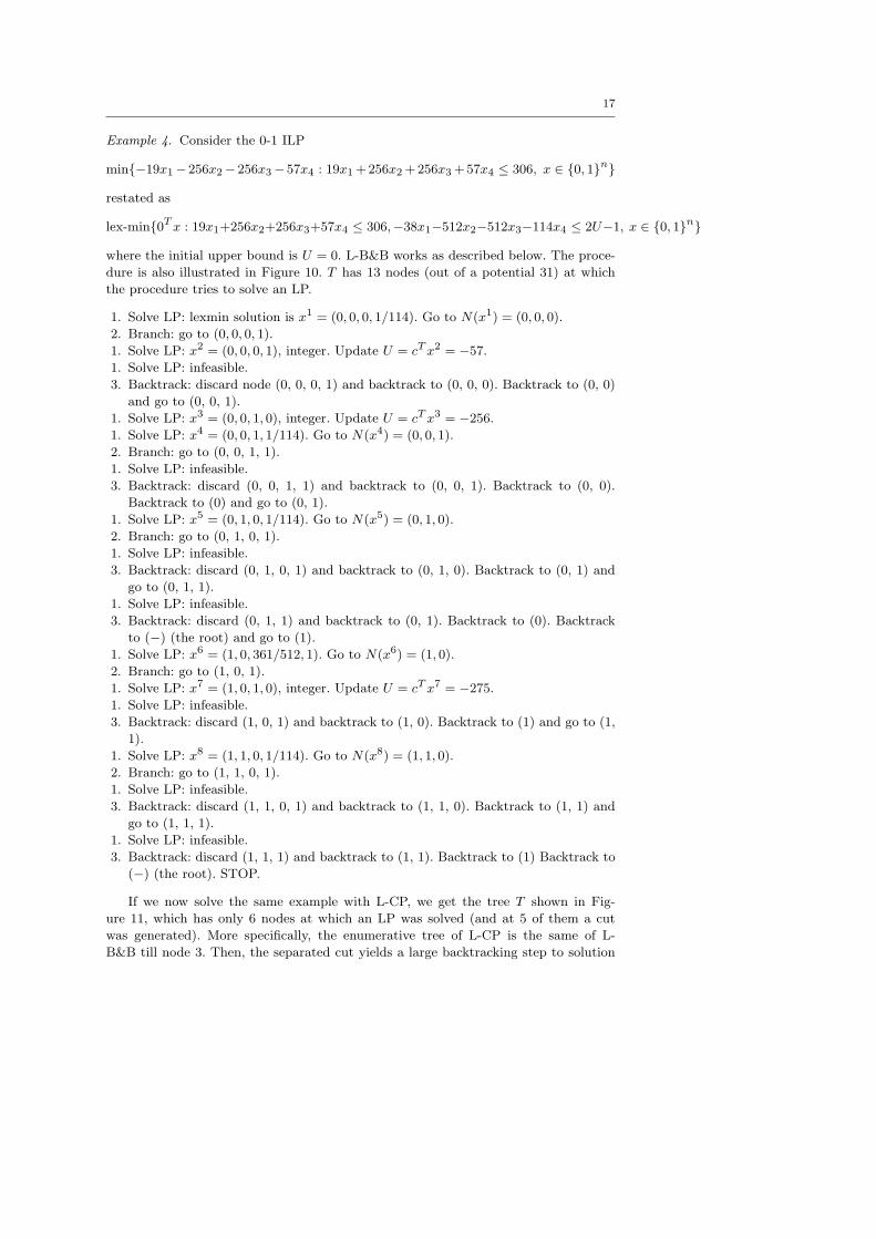
Example 4. Consider the 0-1 ILP

min{−19x1−256x2−256x3−57x4 : 19x1 + 256x2 + 256x3 + 57x4 ≤ 306, x ∈ {0, 1}n}

restated as

lex-min{0T x : 19x1+256x2+256x3+57x4 ≤ 306,−38x1−512x2−512x3−114x4 ≤ 2U−1, x ∈ {0, 1}n}

where the initial upper bound is U = 0. L-B&B works as described below. The proce-

dure is also illustrated in Figure 10. T has 13 nodes (out of a potential 31) at which

the procedure tries to solve an LP.

1. Solve LP: lexmin solution is x1 = (0, 0, 0, 1/114). Go to N(x1) = (0, 0, 0).

2. Branch: go to (0, 0, 0, 1).

1. Solve LP: x2 = (0, 0, 0, 1), integer. Update U = cT x2 = −57.

1. Solve LP: infeasible.

3. Backtrack: discard node (0, 0, 0, 1) and backtrack to (0, 0, 0). Backtrack to (0, 0)

and go to (0, 0, 1).

1. Solve LP: x3 = (0, 0, 1, 0), integer. Update U = cT x3 = −256.

1. Solve LP: x4 = (0, 0, 1, 1/114). Go to N(x4) = (0, 0, 1).

2. Branch: go to (0, 0, 1, 1).

1. Solve LP: infeasible.

3. Backtrack: discard (0, 0, 1, 1) and backtrack to (0, 0, 1). Backtrack to (0, 0).

Backtrack to (0) and go to (0, 1).

1. Solve LP: x5 = (0, 1, 0, 1/114). Go to N(x5) = (0, 1, 0).

2. Branch: go to (0, 1, 0, 1).

1. Solve LP: infeasible.

3. Backtrack: discard (0, 1, 0, 1) and backtrack to (0, 1, 0). Backtrack to (0, 1) and

go to (0, 1, 1).

1. Solve LP: infeasible.

3. Backtrack: discard (0, 1, 1) and backtrack to (0, 1). Backtrack to (0). Backtrack

to (−) (the root) and go to (1).

1. Solve LP: x6 = (1, 0, 361/512, 1). Go to N(x6) = (1, 0).

2. Branch: go to (1, 0, 1).

1. Solve LP: x7 = (1, 0, 1, 0), integer. Update U = cT x7 = −275.

1. Solve LP: infeasible.

3. Backtrack: discard (1, 0, 1) and backtrack to (1, 0). Backtrack to (1) and go to (1,

1).

1. Solve LP: x8 = (1, 1, 0, 1/114). Go to N(x8) = (1, 1, 0).

2. Branch: go to (1, 1, 0, 1).

1. Solve LP: infeasible.

3. Backtrack: discard (1, 1, 0, 1) and backtrack to (1, 1, 0). Backtrack to (1, 1) and

go to (1, 1, 1).

1. Solve LP: infeasible.

3. Backtrack: discard (1, 1, 1) and backtrack to (1, 1). Backtrack to (1) Backtrack to

(−) (the root). STOP.

If we now solve the same example with L-CP, we get the tree T shown in Fig-

ure 11, which has only 6 nodes at which an LP was solved (and at 5 of them a cut

was generated). More specifically, the enumerative tree of L-CP is the same of L-

B&B till node 3. Then, the separated cut yields a large backtracking step to solution

18

1

9

5 11

x3

3 6 8 x710 13

x22 4 7 12

Fig. 10 The lexicographic branch-and-bound method (L-B&B) for a small example.

4

5

1x3

3 x76

x22

Fig. 11 The lexicographic cutting plane method (L-CP) for the same example as in theprevious figure.

(6/161, 31/161, 1, 0), whereas the subsequent two cuts produce solutions (1, 0, 0.8, 1)

and x7 = (1, 0, 1, 0), respectively.

�

We next outline an alternative way to get rid of the objective function. Let lex-GFC

denote the original Gomory dual cutting plane method with lexicographic reoptimiza-

tion and GFCs in their correct ≥ form. The new method, called bin-GFC in the sequel,

consists of embedding lex-GFC in a binary-search scheme that converts the original

19

optimization problem into a sequence of feasibility problems looking for better and

better solutions.

To this end, let [L′, U ′] denote the current objective function interval that corre-

sponds to an integer solution strictly better than the incumbent of value (say) U , where

L′ and U ′ are integer values updated dynamically during the binary search. If L′ > U ′

the incumbent solution is guaranteed to be optimal and we stop.

Otherwise, we apply lex-GFC to find, if any, a (lexicographically minimal) feasible

solution of the original ILP with the objective function replaced by the upper bound

constraint cT x ≤ Utry = b(L′ + U ′)/2c, whose slack variable is put at the bottom

of the lexicographic order. If a solution is found, we update the incumbent value U ,

redefine U ′ = U − 1, and repeat (in this case, we keep in the current ILP model all

the previously-generated cuts, because they will be still valid for the new subproblem

whose feasible set is a subset of that of the previous main iteration). Otherwise, we

update the lower bound L′ = Utry + 1, remove all the previously-generated GFCs, and

repeat.

Note that the method above does not add the lower bound constraint cT x ≥ L′ to

the LP, but only uses value L′ to compute Utry. Indeed, according to our computa-

tional experience the explicit condition cT x ≥ L′ (though mathematically valid in our

context) would actually tend to slow-down the overall computation, due to numerical

issues.

6 Changing the lexicographic order dynamically

According to our computational experience, L-B&B typically generates an unexpect-

edly large number of decision nodes. This behavior is quite surprising as it does not

seem to be explained just by intrinsic inefficiencies related to the depth-first nature

of the lexicographic search, nor by the fact that the branching sequence is fixed be-

forehand. A deeper analysis shows however that there is a crucial issue that heavily

affects the efficiency of every method that makes an explicit or implicit enumeration

on a fixed lexicographic tree: the resort to “unnatural” branchings on integer-valued

variables.

In a typical branch-and-bound run, a large percentage of the decision variables is

likely to stay integer (e.g., nonbasic) during the whole execution, the difficulty of the

instance being related to the remaining “problematic” variables that assume fractional

values or flip during the run. Any sensible branching rule would therefore try to keep

the problematic variables at the top of the branching tree, because otherwise their

fixing would occur down in the tree and hence would be repeated over and over. This

elementary observation is however not taken into account within Gomory-like pure

cutting plane methods, that actually perform (as explained in the previous sections)

a very rigid implicit enumeration of the integer solutions. In other words, Gomory-

like cutting plane methods do need a dynamic rearrangement of the lexicographic

sequence, just as branch-and-bound algorithms need to avoid branching on integer-

valued variables.

The above considerations motivated us to design a new Gomory-like cutting plane

method that uses a dynamic lexicographic order, to be built (and modified) at run-

time. This is in fact possible because of the way we construct the lexicographic optimal

tableau, namely, through a sequence of LP reoptimizations—rather than through a

rigid pivot rule. We next describe in some detail the “dynamic variant” of L-CP, called

20

L-CP.dyn in the sequel. The dynamic variants of lex-GFC (lex-GFC.dyn) and L-B&B

(L-B&B.dyn) can be obtained in an analogous way.

Throughout the algorithm we maintain a partial lexicographic sequence, the vari-

ables outside this sequence having a still-to-be-decided position. The current partial

lexicographic order is represented by a scalar k, giving its length, and by two integer ar-

rays π and V having the following meaning: the current enumeration node corresponds

to fixing xπ[i] = V [i] for i = 1, · · · , k, and it is implicitly assumed that all solutions

x with (xπ[1], · · · , xπ[k]) <LEX (V [1], · · · , V [k]) have been already enumerated. For

instance, for k = 3 we may have xπ[1] = x4 = 0, xπ[2] = x1 = 1, xπ[3] = x5 = 0.

Initially (root node) the sequence is empty, hence k = 0. At each main iteration, we

have a partial lexicographic sequence stored as the triple (k, π, V ) and the current LP

model consisting of a null objective function (recall that the original objective function

cT x is treated implicitly in L-CP) and the original constraints, plus the upper bound

constraint 2cT x ≤ 2U − 1, plus the previously generated GFCs that automatically

ensure that no feasible LP solution x with (xπ[1], · · · , xπ[k]) <LEX (V [1], · · · , V [k])

exists.

We first take a diving step (i.e., a partial lex-optimization step) along the current

partial lexicographic order, that constructs the partial lexicographic optimal tableau

that will generate the GFC. To be specific, for i = 1, 2, · · · , k (in sequence) we perform

the following steps: (i) solve the current LP by using variable xπ[i] as the objective

function to be minimized, and let x be the optimal solution found; (ii) if xπ[i] = V [i],

implicity fix xπ[i] = V [i] by setting to zero all nonbasic variables with positive reduced

cost in the last LP, and proceed with the next position i (if any). At the end of this

loop, if i ≤ k and xπ[i] > V [i] (meaning that the last added GFC yielded a backtracking

step) we shorten the partial sequence by setting k = i− 1.

At this point, the current LP (with some of its variables fixed in their nonbasic

positions) implicitly contains the conditions xπ[i] = V [i] for i = 1, · · · , k, and we

choose our “branching variable” as follows. We put the original objective function

cT x back into the current LP, find an optimal basic solution x∗, and then select a

potential “branching” fractional variable x∗b (b for branching) according to a certain

criterion, e.g., the one whose fractional part is as close as possible to 0.5 or a more

clever rule.2 This step mimics the classical branch-and-bound approach, the difference

being that we actually do not “branch” immediately on xb. Instead, we apply our

lexicographic reoptimization subroutine that discards the original objective function

(cT x) and minimizes xb. If, after reoptimization, variable xb becomes integer in the

new LP solution x (say), we implicitly fix it by setting to zero all nonbasic variables

with positive reduced costs, extend the partial sequence by setting k = k+ 1, π[k] = b,

V [k] = xb, and repeat by looking for another “branching” variable.

At the end of the above branch-selection loop, if all the variables are integer then

a new incumbent has been found, and U is updated along with the associated upper-

bound constraint. Otherwise, we generate a GFC from the tableau row associated with

the “branching” variable xb so as to cut the last fractional point x. In both cases, we

repeat from the diving step above, until the current LP becomes infeasible (meaning

that the current incumbent, if any, is a provably optimal solution).

2 Note that we use notation x∗ for optimal LP solutions with respect to cT x, and notation xfor optimal solutions obtained after lexicographic reoptimizations using some xj as objectivefunction. Also note that the dynamic version of lex-GFC does not need any reoptimization todefine x∗ in that it deals with the objective function through its variable x0, hence x∗ := x.

21

Note that the method above always generates globally-valid GFCs even for general-

integer (as opposed to binary) ILPs—a property that is not easily enforced for the

GFCs typically embedded in a generic branch-and-cut scheme. This is because we

never impose invalid branching conditions on the variables, but we just force some

variables not to belong to the final LP basis that generates the cuts.

The dynamic version of L-B&B, L-B&B.dyn, is obtained in the same way: instead

of using a fixed order of branching, thus allowing for branching even on integer val-

ued variables, the most fractional variable in the current LP solution is used as next

branching variable. It is worth observing that, unlike L-CP vs. L-B&B, the trees under-

lying L-CP.dyn and L-B&B.dyn are typically different because the branching variables

are determined at runtime with respect to different LP solutions, so there is no strict

dominance between the two.

7 Computational experiments

We ran some computational experiments to evaluate some main variants of the Gomory

cutting plane procedure. To this end, we implemented the original Gomory dual cutting

plane method with lexicographic reoptimization and GFCs in their correct ≥ form (lex-

GFC, as described in section 3 and implemented in [17]), as well as the lexicographic

cutting plane (L-CP), the lexicographic branch-and-bound (L-B&B), and the binary-

search (bin-GFC) methods described in the previous sections, along with their dynamic

(.dyn) versions described in Section 6.

For all methods, the lexicographic sequence of LP reoptimizations needed at each

main iteration to get a lex-optimal tableau is stopped as soon as the current variable

xh receives a fractional value x∗h after reoptimization, thus saving the subsequent re-

optimization calls for xh+1, · · · , xn that would not change the tableau row having xhas basic variable, and hence would have no effect on the GFC generated from this row.

In addition, we use a multi-cut separation strategy that generates all the GFCs that

can be read from the final tableau, and not just the first one that would be enough

for the convergence proof. It is easy to see that this does not affect the finiteness of

the procedure. On the other hand, the addition of “rounds of cuts” tends to improve

the numerical stability of the overall method and to accelerate convergence—though

the speedup is not as dramatic as in a branch-and-cut context where lexicographically

non-optimal tableaux are used to derive the cuts.

All algorithms have been coded in C++ and run on a PC Intel Core 2 Q6600,

2.40GHz, with a time limit of 2 hours of CPU time and a memory limit of 2GB for

each instance. ILOG Cplex 11 with default parameters has been used as LP black-box

solver. All reported times are in CPU seconds.

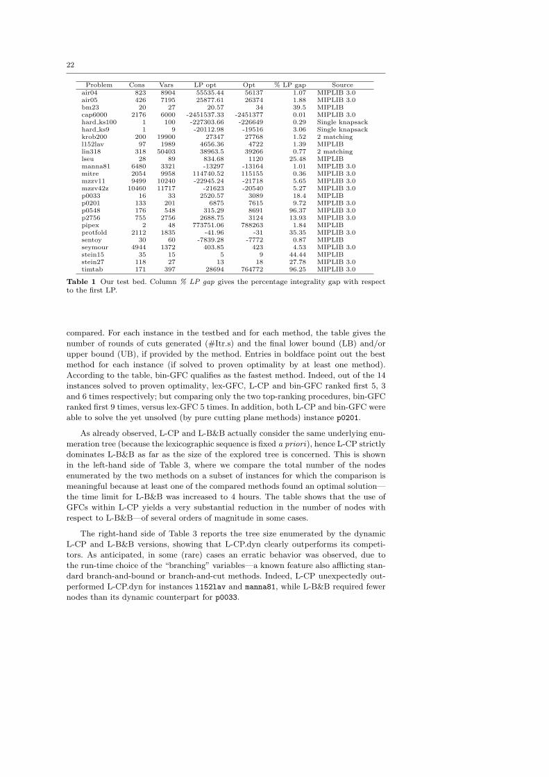
Our testbed is the same as in [17], and consists of 25 pure ILP instances coming

from MIPLIB 3 and 2003 [5,1]; see Table 1. As our computational analysis is aimed at

comparing the performance of different cutting plane approaches, we did not include

in the testbed some difficult instances that are likely not to be solvable by any pure

cutting plane method. It is worth noting, however, that even very small instances of

our testbed (e.g., stein15 and bm23) have never before been solved by a pure cutting

plane method based on GFC or GMI cuts read from the LP tableau [17].

Table 2 reports the outcome of a first experiment aimed at evaluating the effect of

getting rid of the objective function (without exploiting a the dynamic rearrangement

of the lexicographic sequence) . Three methods (lex-GFC, L-CP, and bin-GFC) are

22

Problem Cons Vars LP opt Opt % LP gap Sourceair04 823 8904 55535.44 56137 1.07 MIPLIB 3.0air05 426 7195 25877.61 26374 1.88 MIPLIB 3.0bm23 20 27 20.57 34 39.5 MIPLIBcap6000 2176 6000 -2451537.33 -2451377 0.01 MIPLIB 3.0hard ks100 1 100 -227303.66 -226649 0.29 Single knapsackhard ks9 1 9 -20112.98 -19516 3.06 Single knapsackkrob200 200 19900 27347 27768 1.52 2 matchingl152lav 97 1989 4656.36 4722 1.39 MIPLIBlin318 318 50403 38963.5 39266 0.77 2 matchinglseu 28 89 834.68 1120 25.48 MIPLIBmanna81 6480 3321 -13297 -13164 1.01 MIPLIB 3.0mitre 2054 9958 114740.52 115155 0.36 MIPLIB 3.0mzzv11 9499 10240 -22945.24 -21718 5.65 MIPLIB 3.0mzzv42z 10460 11717 -21623 -20540 5.27 MIPLIB 3.0p0033 16 33 2520.57 3089 18.4 MIPLIBp0201 133 201 6875 7615 9.72 MIPLIB 3.0p0548 176 548 315.29 8691 96.37 MIPLIB 3.0p2756 755 2756 2688.75 3124 13.93 MIPLIB 3.0pipex 2 48 773751.06 788263 1.84 MIPLIBprotfold 2112 1835 -41.96 -31 35.35 MIPLIB 3.0sentoy 30 60 -7839.28 -7772 0.87 MIPLIBseymour 4944 1372 403.85 423 4.53 MIPLIB 3.0stein15 35 15 5 9 44.44 MIPLIBstein27 118 27 13 18 27.78 MIPLIB 3.0timtab 171 397 28694 764772 96.25 MIPLIB 3.0

Table 1 Our test bed. Column % LP gap gives the percentage integrality gap with respectto the first LP.

compared. For each instance in the testbed and for each method, the table gives the

number of rounds of cuts generated (#Itr.s) and the final lower bound (LB) and/or

upper bound (UB), if provided by the method. Entries in boldface point out the best

method for each instance (if solved to proven optimality by at least one method).

According to the table, bin-GFC qualifies as the fastest method. Indeed, out of the 14

instances solved to proven optimality, lex-GFC, L-CP and bin-GFC ranked first 5, 3

and 6 times respectively; but comparing only the two top-ranking procedures, bin-GFC

ranked first 9 times, versus lex-GFC 5 times. In addition, both L-CP and bin-GFC were

able to solve the yet unsolved (by pure cutting plane methods) instance p0201.

As already observed, L-CP and L-B&B actually consider the same underlying enu-

meration tree (because the lexicographic sequence is fixed a priori), hence L-CP strictly

dominates L-B&B as far as the size of the explored tree is concerned. This is shown

in the left-hand side of Table 3, where we compare the total number of the nodes

enumerated by the two methods on a subset of instances for which the comparison is

meaningful because at least one of the compared methods found an optimal solution—

the time limit for L-B&B was increased to 4 hours. The table shows that the use of

GFCs within L-CP yields a very substantial reduction in the number of nodes with

respect to L-B&B—of several orders of magnitude in some cases.

The right-hand side of Table 3 reports the tree size enumerated by the dynamic

L-CP and L-B&B versions, showing that L-CP.dyn clearly outperforms its competi-

tors. As anticipated, in some (rare) cases an erratic behavior was observed, due to

the run-time choice of the “branching” variables—a known feature also afflicting stan-

dard branch-and-bound or branch-and-cut methods. Indeed, L-CP unexpectedly out-

performed L-CP.dyn for instances l152lav and manna81, while L-B&B required fewer

nodes than its dynamic counterpart for p0033.

23

Lex-GFC L-CP Bin-GFCInstance #Itr.s Time LB #Itr.s Time UB #Itr.s Time LB UB

air4 434 7207 55687 19 7761.37 – 22 7500 – –air5 833 7209 26003 172 7218.49 – 151 7208 – –bm23 660 2 ? 836 2.65 ? 357 0.82 ? ?cap6000 16043 7201 -2451485 19339 7201.29 -145849 12490 7201 2451541 -1266187hard ks100 99 0.43 ? 8089 16.67 ? 345 0.51 ? ?hard ks9 141 0.22 ? 81 0.07 ? 83 0.05 ? ?krob200 41 93.94 ? 445 7228.16 312340 293 1901 ? ?l152lav 744 118.2 ? 5214 705.22 ? 2304 125.61 ? ?lin318 28 200.08 ? 111 7378.44 816595 29 7561 38965 428586lseu 9591 53.24 ? 42160 199.6 ? 2600 10.89 ? ?manna81 12 19.05 ? 16640 2991.28 ? 2542 1307 ? ?mitre 565 7209 115117 239 7204.77 133920 246 7240 114742 134160mzzv11 16 8533 -22566.5 297 7227.45 -2518 34 7224 22946 0mzzv42z 19 7519 -21434 233 7219.34 -2828 51 7279 21623 0p0033 501 1.2 ? 106 0.16 ? 51 0.1 ? ?p0201 190383 7201 7521 5574 117.79 ? 6672 125.44 ? ?p0548 129823 7201 6753 172771 7201.02 28953 144918 7201 317 40214p2756 51454 7201 3036 42973 7201.25 5353 30122 7201 2690 7160pipex 473607 1591.97 ? 2251 9.01 ? 942 3.45 ? ?protfold 144 7253 -37 178 7237.26 – 153 7260 1 –sentoy 5338 24.36 ? 32759 114.56 ? 2541 10.57 ? ?seymour 117 7224 409 1925 7203.61 469 671 7423 405 502stein15 68 0.15 ? 56 0.10 ? 67 0.11 ? ?stein27 3134 13.96 ? 1993 6.58 ? 2840 6.64 ? ?timtab 5193 7344 399948 66684 7201.13 1063711 22765 7201 28695 1129107

Table 2 Comparison between different versions of the Gomory cutting plane method (? meanssolved to proven optimality).

L-CP L-B&B L-CP.dyn L-B&B.dynInstance Time Nodes Time Nodes Time Nodes Time Nodes

bm23 2.65 2,205 0.29 3,372 0.96 1,013 0.13 1,358hard ks100 16.67 41,303 7200 >122,828,201 15.18 24,077 4084 56,872,670hard ks9 0.07 164 0.01 ,274 0.05 133 0.01 228l152lav 705.22 1,111,733 1876 3,335,512 7201 >634,042 1406 1,354,164lseu 199.6 191,256 1153 15,089,374 46.59 23,327 12.38 109,578manna81 2991.28 142,013 7200 >3,321,404 7202 > 8,276 7200 >2,692,153p0033 0.16 380 0.62 11,538 0.17 307 0.83 12,192p0201 117.79 58,101 59.07 357,664 38.56 11,127 6.51 26,942pipex 9.01 6,474 1.31 13,904 2.83 2,198 0.72 7,686sentoy 114.56 103,349 20.04 197,510 2.39 1,460 0.16 2,038stein15 0.1 123 0.03 418 0.11 97 0.02 260stein27 6.58 4,160 1.62 13,260 6.47 3,551 1.22 9,210

Table 3 Comparison between the tree size (total number of the nodes) enumerated by L-CP, L-B&B, and by their dynamic (.dyn) versions (in boldface, the version requiring theminimum number of nodes).

Finally, we compare in Table 4 the performance of the two cutting plane methods

not using invalid cuts, namely: the standard lex-GFC, as implemented in [17], and

its new dynamic version introduced in the present paper. Each run is marked by its

termination code: O for proven optimality, T for time limit, E for numerical errors,

and C for 10,000,000-cut limit exceeded. For each instance in the testbed, we report

in boldface the figure defining the best method—percentage closed gap (%Cl.Gap),

or computing time (Time) in case of ties. It turns out that lex-GFC.dyn performs

significantly better than lex-GFC, in that it was the best of the two in 18 out of 25

24

Lex-GFC Lex-GFC.dynInstance #Itr.s Cuts Time %Cl.Gap #Itr.s Cuts Time %Cl.Gap

air4 T 434 140191 7207 25.19 T 559 178404 7218 36.17air5 T 833 240266 7209 25.26 T 1119 321186 7209 30.7bm23 O 660 8294 2 100 O 652 8047 0.99 100cap6000 T 16043 107239 7201 32.64 T 76649 493654 7201 83.16hard ks100 O 99 483 0.43 100 O 809 4100 2.73 100hard ks9 O 141 609 0.22 100 O 130 542 0.08 100krob200 O 41 1643 93.94 100 O 23 375 18.64 100l152lav O 744 25109 118.2 100 T 42184 1911790 7201 86.29lin318 O 28 1001 200.08 100 O 27 848 67.79 100lseu O 9591 133589 53.24 100 O 4261 53522 11.75 100manna81 O 12 280 19.05 100 O 12 280 12.63 100mitre T 565 116369 7209 90.83 O 786 132399 6125 100mzzv11 T 16 14516 8533 30.86 T 28 23496 7409.5 37.18mzzv42z T 19 15264 7519 17.45 T 31 24081 7550 23.14p0033 O 501 4421 1.2 100 O 1214 10622 2.12 100p0201 T 190383 5471004 7201 87.3 T 259143 8984687 7201 96.49p0548 T 129823 4832247 7201 76.86 T 12412 450566 110781 53.21p2756 T 51454 673642 7201 79.78 E 134 7550 7.35 79.78pipex O 473607 4583701 1592 100 C 1081606 >10000000 2219 97.51protfold T 144 57617 7253 45.26 T 253 94771 7203 36.13sentoy O 5338 68991 24.26 100 O 3170 40765 6.52 100seymour T 117 67931 7224 26.89 T 149 84533 7217 32.11stein15 O 68 708 0.15 100 O 59 641 0.10 100stein27 O 3134 35861 13.96 100 O 2250 27462 5.63 100timtab T 5193 1675111 7344 50.44 T 4090 1320383 7550 46.37

Table 4 Effect of dynamic lexicographic reorder: lex-GFC vs. lex-GFC.dyn

cases. Note that lex-GFC.dyn was not able to solve instances l152lav and pipex that

were on the other hand solved by lex-GFC, while the opposite held for mitre.

8 Conclusions

We have addressed important issues arising when designing a computationally sound

cutting plane method for pure integer problems. In particular, we have analyzed the

dual cutting plane procedure proposed by Gomory in 1958, which is the first (and most

famous) convergent cutting plane method for Integer Linear Programming.

In a previous work [17], we pointed out the practical importance of using Gomory

fractional cuts (GFCs) together with the lexicographic dual method—in a pure cutting

plane context, GFCs and the lexicographic method are the two blades of a pair of

scissors.

In the present paper, the enumerative nature of Gomory’s method has been de-

scribed with the help of detailed examples. So far, this known property was mainly

used as a theoretical tool leading to an elegant proof of convergence. Instead, we have

pointed out the practical importance of the enumerative interpretation: since Gomory’s

method is in fact cast in its enumerative framework, its performance can only be im-

proved if one gets rid of the rigidity of the enumerative shell.

We have therefore proposed and computationally analyzed new versions of the

Gomory method, that borrow from native enumerative schemes some of their main

features. In particular, we have analyzed cutting plane algorithms where the objective

function is treated implicitly, and/or the lexicographic order is redefined on the fly to

25

mimic a sound branching strategy. Preliminary computational results seem to indicate

that the new methods have some potential.

Future research should try to put even more flexibility in pure cutting plane meth-

ods. In doing so, we expect that a better understanding of the interaction between cuts

and enumeration will be gained, with a positive follow-up for the branch-and-cut side

too.

References

1. T. Achterberg, T. Koch, and A. Martin. MIPLIB 2003. Operations Research Letters,34:361–372, 2006. Problems available at http://miplib.zib.de.

2. J. L. Arthur and A. Ravindran. PAGP, a partitioning algorithm for (linear) goal program-ming problems. ACM Trans. Math. Softw., 6(3):378–386, 1980.

3. E. Balas and A. Saxena. Optimizing over the split closure. Mathematical Programming,113(2):219–240, 2008.

4. M. L. Balinski and A. W. Tucker. Duality theory of linear programs: A constructiveapproach with applications. SIAM Review, 11(3):347–377, July 1969.

5. R. E. Bixby, S. Ceria, C. M. McZeal, and M. W. P Savelsbergh. An updated mixed integerprogramming library: MIPLIB 3.0. Optima, (58):12–15, June 1998.

6. I. Borg and P.J.F. Groenen. Modern Multidimensional Scaling: Theory and Applications.Springer, 2005.

7. V. Chvatal. Edmonds polytopes and a hierarchy of combinatorial problems. DiscreteMathematics, 4:305–337, 1973.

8. W. Cook, R. Kannan, and A. Schrijver. Chvatal closures for mixed integer programmingproblems. Mathematical Programming, 47:155–174, 1990.

9. S. Dash, O. Gunluk, and A. Lodi. MIR closures of polyhedral sets. Mathematical Pro-gramming, 121:33–60, 2010.

10. M. Fischetti and A. Lodi. Optimizing over the first Chvatal closure. Mathematical Pro-gramming B, 110(1):3–20, 2007.

11. R. E. Gomory. Outline of an algorithm for integer solutions to linear programs. Bulletinof the American Society, 64:275–278, 1958.

12. R. E. Gomory. An algorithm for the mixed integer problem. Technical Report RM-2597,The RAND Cooperation, 1960.

13. R. E. Gomory. An algorithm for integer solutions to linear programming. In R. L. Gravesand P. Wolfe, editors, Recent Advances in Mathematical Programming, pages 269–302,New York, 1963. McGraw-Hill.

14. G. Nemhauser and L. Wolsey. Integer and combinatorial optimization. Wiley, 1988.15. F.J. Nourie and E.R. Venta. An upper bound on the number of cuts needed in Gomory’s

method of integer forms. Operations Research Letters, 1:129–133, 1982.16. M. Tamiz, D. F. Jones, and E. El-Darzi. A review of goal programming and its applications.

Annals of Operations Research, 58(1):39–53, 1995.17. A. Zanette, M. Fischetti, and E. Balas. Lexicography and degeneracy: Can a pure cutting

plane algorithm work? Mathematical Programming, 2010 (to appear).