On the emergence of flocking in birds

Adam Bauer∗

May 9, 2021

Abstract

This essay will provide a brief overview of the many approaches scientists have taken to

study bird flocking, including numerical, observational, and analytic methods. We discuss

the pioneering work first done in numerical modeling and theoretical physics, and how these

approaches are challenged by observational data. Lastly, we discuss an observationally

motivated theoretical framework for studying flocking.

Contents

1 Introduction 1

2 Numerical models 1

3 Early theoretical model: the Vicsek model 2

3.1 Alterations to the Vicsek model . . . . . . . . . . . . . . . . . . . . . . . . . . . 5

4 Observational data 5

5 Topological models of flocking 9

6 Summary 11

“ ... and the thousands of fishes moved as a huge beast, piercing the water. They appeared

united, inexorably bound to a common fate. How comes this unity?” – Anonymous, 17th

century [10]

∗Department of Physics, University of Illinois Urbana-Champaign, 1110 W Green St Loomis Laboratory,

Urbana, IL 61801

1 Introduction

The existence of collective behavior in nature has been the fascination of scholars for generations.Indeed, whether it was Ernst Ising modeling ordered magnetic systems or Friedrich Hayekconsidering “natural order” and its relation to law, the concepts of “order” and “disorder”consistently capture the attention of academics across disciplines. In particular, physicists andmathematicians have spearheaded the pursuit to analyze the existence and behavior of orderedstructures in mathematical models of natural phenomena.

One such phenomena that has garnered considerable attention from both the physics and math-ematics communities is flocking: the collective, synchronized movement of large collections ofself-organizing agents. Flocking is ubiquitous in nature, and can be observed in organisms suchas birds and sheep, as well as in schools of fish. Some flocking phenomena, such as starling mur-murations, can consist of thousands of birds, all flying in unison [1]. In this essay, we will focusspecifically on bird flocking, but the reader should remain aware that the material discussedherein is applicable to many of the examples given above.

Despite the commonplace nature of bird flocking, formulating a consistent model of flockingremains a difficult and interdisciplinary challenge for scientists. Indeed, until recently little ob-servational data had been taken, making key model parameters difficult to estimate from fielddata. In the absence of data, computational scientists designed minimal models that repro-duced flocking behavior in numerical experiments, marking the first step of progress towardsunderstanding flocks [10]. Theoretical physicists also managed to make headway on developingmodels that predicted phase transitions within bird flocks [11]. However, a recent breakthroughobservational study of bird flocking [2] led to the discovery of a topological interaction betweenbirds, calling the assumptions of early numeric and theoretical models into serious question [1].Since this study, models based on topological interactions have been formulated that reproduceflocking and predict the propagation of order throughout the flock with no free parameters [3].

In this essay, we intend to delve into the challenges in modeling bird flocking, as well as theprogress made towards understanding emergent collective behavior in these systems. In §2, wewill give an overview of the early numerical methods used to study bird flocking. In §3, we willdiscuss the first theoretical model of bird flocking and its associated phase transition. We willbriefly touch on the modifications to this model in §3.1. In §4, we will discuss the observationalrecord of bird flocking, and how recent observational studies have caused breakthroughs in ourunderstanding of flocking. Lastly, we will discuss a new analytic theory of bird flocking in §5which is based off of the topological interaction between birds discovered in [1]. We close witha summary in §6.

2 Numerical models

Given the lack of observational data on flocking, computational science was the first disciplineto make real progress on studying the collective behavior of natural systems. The first computermodel where emergent flocking was observed was developed by Reynolds, who endowed eachindependent particle moving along a three dimensional (3D) path with a distributed behaviormodel that led to collective flocking behavior [10]. Note that the “particles” within the simula-tion are meant to be interpreted as birds (called “bird-oids,” cutely nicknamed “boids” in the

1

paper). The behavioral model that dictated the behavior of each boids’ local dynamics had thefollowing tenants, listed in order of decreasing precedence:

1. Collision avoidance: avoid collisions with nearby flockmates;

2. Velocity matching: attempt to match velocity with nearby flockmates;

3. Flock centering: attempt to stay close to nearby flockmates. [10]

Figure 1: The 3D animated flock of boidsproduced in [10]. The point of the boids in-dicates flight direction.

Simulations were initialized with random loca-tions and velocities for all boids within a spec-ified domain. After an initial “expansion burst,”where the rule of avoiding collisions dominatedthe system, flocks of boids developed by followingthe behavioral model laid out above, see Figure 1for an example. Additionally, the flocks observedwere “polarized,” in the sense that velocities werematched in both direction and speed, and wereable to bifurcate around a static obstacle, as isobserved in real flocks. In summary, simulatedflocks demonstrate what the author describes asbehavior “corresponding to the observer’s intu-itive notion of what constitutes ‘flock-like mo-tion’” [10].

Models have built on the framework above toprobe flocking at deeper levels. For example, in [8], Heppner and Grenander use a set of phys-ically motivated nonlinear stochastic differential equations to model boids’ flight paths, whichresulted in flocking. In this set of equations, there existed terms that accounted for each of therules listed above, as well as a term that accounted for the location of a roost (that attractedthe flock) and some random Poisson noise, that was meant to simulate the impact of wind andother external perturbations. Strikingly, this model only produces flocking (over the roostinglocation) for some set of parameters ; for other sets of parameters, no synchronized flock forms,and the group of boids resembles a “swarm of gnats” [8]. This suggests that flocking is a behav-ior that only exists for a certain set of parameter values, a concept we will revisit later in thisreport (see §3).Reynolds, Heppner and Grenander all readily admit that while their simulations were successful,it is difficult to objectively verify how well the simulated flocks compare with flocks in nature [8,10]. This reality raised the demand for observational data of flocks to compare with simulations.A similar problem was encountered in the theoretical community, discussed in the next section.

3 Early theoretical model: the Vicsek model

The Vicsek model (VM) is a first-of-its-kind numerical model of self-propelled agent basedflocking put forth in 1995 [11]. The model consists of polar point particles on a 2D plane.These particles’ motion is kept at constant velocity, and are allowed to move in any direction.The direction in which they move is updated at each timestep in the simulation by the average

2

velocity of other agents that are within its “domain of influence,” defined in this case as a sphereof unit radius around the particle. This model was shown to exhibit a phase transition, due tothe spontaneous breaking of rotational symmetry.

Let us put the above into a mathematical framework. Consider N particles on a 2D plane withside length L. As discussed above, the ith particle moves at constant speed v at an angle ϑi(t)with the x -axis. Therefore, at time t+ 1, the particle position is given by

xi(t+ 1) = xi(t) + vi(t)∆t, (3.1)

wherevi(t) = veiϑi(t), (3.2)

is the velocity at time t. As we progress in time, v remains constant, but ϑi(t) must be updatedto account for the influence of other agents. At the following timestep in the simulation, wetherefore compute ϑi(t+ 1) as

ϑi(t+ 1) = ⟨ϑi(t)⟩r + δϑi, (3.3)

where ⟨ϑi(t)⟩r is the average angle of travel for all particles within a radius r from particlei (including the ith particle), and δϑi is a random number chosen such that −η/2 ≤ δϑi ≤η/2, where η ∈ R+ is an adjustable noise parameter. This is done to prevent against perfectalignment. Following the above prescription, VM has three free parameters: the density, ρ =N/L2, the noise parameter, η, and v, the amount of distance covered by an agent in a timestep.

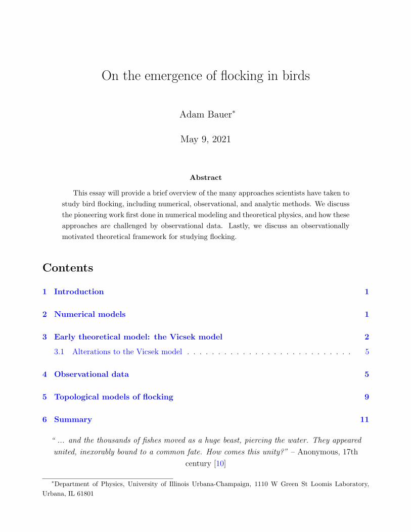
Simulations in [11] were carried out by fixing v = 0.03, and allowing η and ρ to vary. Initiallya number of particles N were generated with random positions and directions. For low densityand noise, the particles formed coherent small groups that moved in random directions. For highdensity and high noise the system was entirely randomly moving with very little correlation.When the density is large and the noise is small, the motion becomes ordered on a macroscopicscale and all agents tend to move in the same “spontaneously selected” direction [11]. See Figure2 for examples of these cases, panels (b)–(d), respectively.

This spontaneous ordering signals a phase transition in the model from a disordered state (panels(a) – (c) of Figure 2) to an ordered state (Figure 2 panel (d)). To investigate this transition,Vicsek et al. define the average, normalized velocity va as

va :=1

Nv

∣∣∣∣ N∑i=1

vi

∣∣∣∣. (3.4)

Note if the system is entirely random, va → 0, and if the system is completely coherent, va → 1,thus making va an order parameter. Vicsek et al. find that for various values of the noise anddensity, the order parameter va behaves much like that of an order parameter of some equilibriumsystems near the critical point, even though the system they consider is not in equilibrium. SeeFigure 2, panel (e) ((f), resp.) for the behavior of va with respect to η (ρ, resp.). They postulatethis is because the agents are diffusing, which causes mixing, thus resulting in an effectivelong-range interaction radius [11].

Vicsek et al. derive a scaling law for the order parameter va in terms of the density and noise

3

Figure 2: For panels (a) – (d), arrows indicate the agent direction of motion, and small curvesshow the agent location for the previous 20 timesteps. (a). Simulation results at t = 0. (b).Simulation results when density and noise are small. (c). Simulation results when densityand noise is high. (d). Simulation results when density is high and noise is small; notice themacroscopic ordering in the system. (e). The order parameter va as a function of η for differentparticle numbers. (f). The order parameter va as a function of ρ. (Images taken from [11].)

in the thermodynamic limit (L → ∞), such that

va ∼ (ηc(ρ)− η)β , va ∼ (ρ− ρc(η))δ , (3.5)

where β, δ are the critical exponents and ηc(ρ) and ρc(η) are the critical noise and density in thethermodynamic limit, respectively. Vicsek et al. compute the critical exponents by regressingln va against ln ((ηc(L)− η) /ηc(L)) and ln ((ρ− ρc(L)) /ρc(L)) for some fixed values of ρ andη, respectively. They compute β = 0.45 ± 0.07 and δ = 0.35 ± 0.06 [11]. As noted above, ηcdepends on ρ, and Vicsek et al. predict the phase diagram for their model to be a line of criticalη values, analogous to ferromagnets. This would indicate that the phase transition occurring inthis model is of second order [11].

VM was the first successful model to predict a phase transition in self-propelled agent models.Since, VM has been built on, leading to new predictions. We discuss one such alteration in thenext subsection.

4

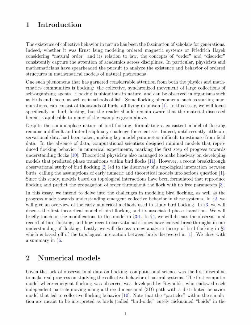
Figure 3: A typical flock and its 3D reconstruction. (a, b) Left-hand and right-hand, photos ofthe stereo pair, taken at the same time, but 25 m apart. (c,e,f) 3D reconstruction of the flockin the reference frame of the right-hand camera, under four different points of view. (d) Showsthe reconstructed flock with the same perspective as (b). (Figure taken directly from [2].)

3.1 Alterations to the Vicsek model

One alteration made to VM in [6] was to limit the range of perception of each individual birdto a slice of a disk instead of a full disk, as was used in VM. This had a substantial impact onthe result of the numerical simulation. The numerical studies done in [6] were carried out in thefollowing way. They simulated the flight of N birds in 2D, as was done in VM, but with theaverage influence on ϑi only being averaged over a subset of a disk of radius r, such that (3.3)is changed such that

ϑi(t+ 1) = ⟨ϑi(t)⟩Ξ + δϑi, (3.6)

where Ξ ⊂ R2 is a subset of the unit disk. The size of Ξ was varied for each simulation and wasparameterized by a “viewing angle,” that modeled the extent of a given bird’s visual perception.The same order parameter as in VM was studied here. Remarkably, the critical viewing anglefor large system sizes was approximately ϕc ≈ 0.2π, or ϕc ≈ 35◦. This had a substantial impacton the result of the numerical simulation; in VM, the phase transition experienced in the modelwas of second order; in the modified case, the transition is first order.

However, just as was the case with early numerical models, VM and its alternatives were notmotivated by any observational data, but rather by intuitive notions of biological interaction. Asthe theoretical and numerical study of flocking advanced, the demand for thorough observationalinvestigation grew; this demand was eventually met by Ballerini and her collaborators in 2007,finally presenting an opportunity for theory to be checked by real-world observations.

4 Observational data

Although bird flocking is readily observable with our eyes, capturing the behavior on scientificinstruments has been a consistent challenge. Field observations, prior to 2007, suffered from

5

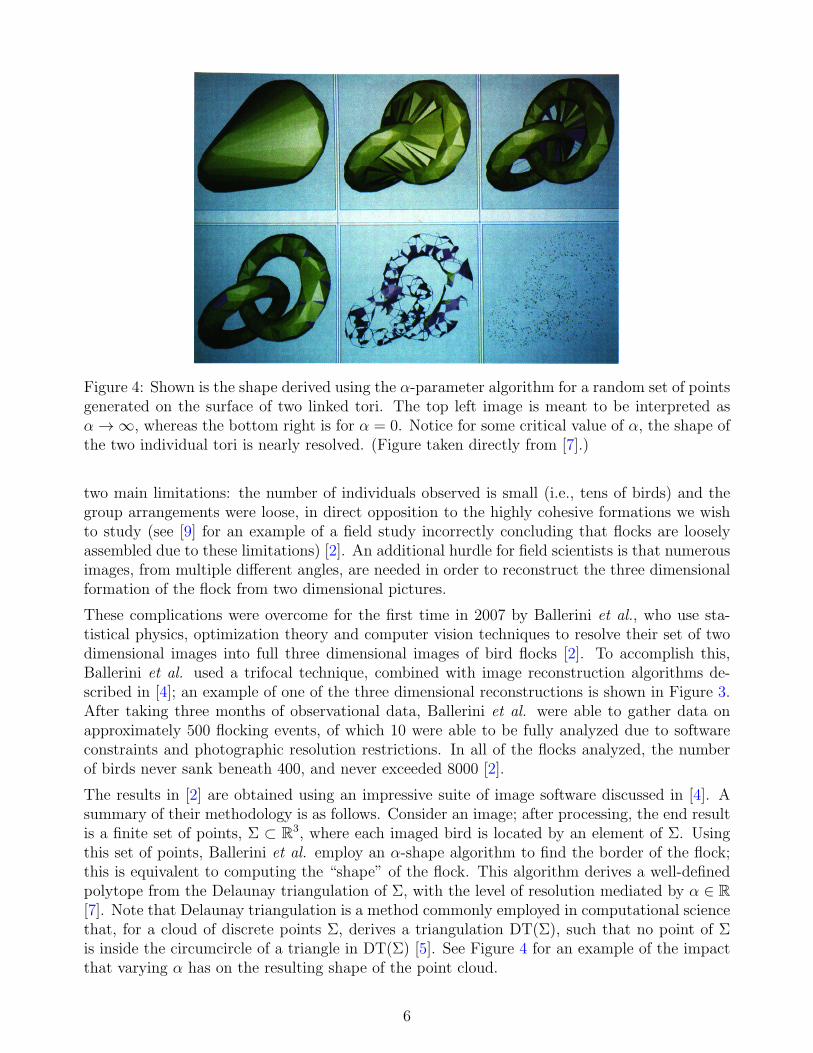
Figure 4: Shown is the shape derived using the α-parameter algorithm for a random set of pointsgenerated on the surface of two linked tori. The top left image is meant to be interpreted asα → ∞, whereas the bottom right is for α = 0. Notice for some critical value of α, the shape ofthe two individual tori is nearly resolved. (Figure taken directly from [7].)

two main limitations: the number of individuals observed is small (i.e., tens of birds) and thegroup arrangements were loose, in direct opposition to the highly cohesive formations we wishto study (see [9] for an example of a field study incorrectly concluding that flocks are looselyassembled due to these limitations) [2]. An additional hurdle for field scientists is that numerousimages, from multiple different angles, are needed in order to reconstruct the three dimensionalformation of the flock from two dimensional pictures.

These complications were overcome for the first time in 2007 by Ballerini et al., who use sta-tistical physics, optimization theory and computer vision techniques to resolve their set of twodimensional images into full three dimensional images of bird flocks [2]. To accomplish this,Ballerini et al. used a trifocal technique, combined with image reconstruction algorithms de-scribed in [4]; an example of one of the three dimensional reconstructions is shown in Figure 3.After taking three months of observational data, Ballerini et al. were able to gather data onapproximately 500 flocking events, of which 10 were able to be fully analyzed due to softwareconstraints and photographic resolution restrictions. In all of the flocks analyzed, the numberof birds never sank beneath 400, and never exceeded 8000 [2].

The results in [2] are obtained using an impressive suite of image software discussed in [4]. Asummary of their methodology is as follows. Consider an image; after processing, the end resultis a finite set of points, Σ ⊂ R3, where each imaged bird is located by an element of Σ. Usingthis set of points, Ballerini et al. employ an α-shape algorithm to find the border of the flock;this is equivalent to computing the “shape” of the flock. This algorithm derives a well-definedpolytope from the Delaunay triangulation of Σ, with the level of resolution mediated by α ∈ R[7]. Note that Delaunay triangulation is a method commonly employed in computational sciencethat, for a cloud of discrete points Σ, derives a triangulation DT(Σ), such that no point of Σis inside the circumcircle of a triangle in DT(Σ) [5]. See Figure 4 for an example of the impactthat varying α has on the resulting shape of the point cloud.

6

Once the border was defined, the volume of the flock was computed using the Delaunay triangu-lation, only considering birds internal to the border. The dimensions of the flock were derived inthe following way. The thickness, I1, was defined as the diameter of the largest sphere containedwithin the flock’s boundary. Exploiting the fact that the thickness is the shortest dimension ofthe flock by construction (see panel (c) of Figure 3), a plane was fitted to the flock, with the

axis orthogonal to the plane being labeled as I1. The second dimension I2 was defined as thediameter of the smallest circle contained in the 2D projection of the flock onto the plane; the2D projection was then fit to a line, which defined the third dimension I3. The axis I2 was thenfound by completing the 3D orthogonal basis containing the other axes I1 and I3 [2].

The main results from their analysis is the following. Ballerini et al. measured the aspect ratiosof the flock with respect to the thickness I1, i.e., the quantities I2/I1 and I3/I1. The averageover all events was found to be I2/I1 = 2.8± 0.4 and I3/I1 = 5.6± 1.0, where they report 95%confidence intervals [2]. These results confirm what was visually represented in Figure 3 panel(c), that flocks are generally thin in one dimension and prefer to spread out laterally. Thisfinding is supported by their analysis on the orientation of the flock. Defining g as the unitvector pointing in the direction of gravity and v as the unit vector pointing in the direction ofthe flock’s center of mass velocity, Ballerini et al. find that, on average, |I1 · g| = 0.93 ± 0.04,

whereas |v · g| = 0.13±0.05 and |v · I1| = 0.19±0.08 [2]. The conclusion we can draw from thesefindings is that flocks tend to align their thinnest dimension along the vertical axis (i.e., parallelto gravity), and as a unit move parallel to the Earth’s surface. This can easily be explained viaenergetic considerations; there is a higher energy cost to oppose gravity and fly in the verticaldirection, therefore it is more energetically favorable for the flock to fly parallel to the ground.Also, this supports the assumption that 2D models can accurately reproduce realistic flockingbehavior, as was done in [11, 6].

Another important result is that the density of flocks varied substantially, and did not depend onthe number of birds belonging to the flock [2]. Furthermore, the nearest neighbor distance alsodid not depend on the size of the group, which is contrary to patterns observed in fish schoolsand in numerical simulations. This result was analyzed further by Ballerini and her collaboratorsin [1], where they found that the interaction between birds does not depend on metric distance(as most models assume1), but on the topological distance. This implies a stunning conclusion:the “attraction” between two birds depends on the number of individual birds that separatethem, rather than the physical distance away; so long as there are no birds in between a pair ofbirds, it matters not whether they are separated by 1 m or 10 m. Ballerini et al. reports thaton average, individual birds interact with about six to seven of their nearest neighbors [1].

The methodology used in [1] to reach this conclusion is as follows. For each bird in an imagedflock, Ballerini et al. measure the angular orientation of its nearest neighbor with respect to theflock’s direction of motion, i.e., the neighbor’s bearing and elevation. This is done for both thenearest neighbor and the tenth closest bird to the reference bird; see Figure 5. The results inFigure 5 are derived by assigning a unit vector ui for the ith bird in the direction of its nearestneighbor. Each unit vector is placed at the origin, and the density normalized by the isotropiccase is plotted on the unitary sphere. Ballerini et al. note that this anisotropic pattern continuesif one plots the second nearest neighbor, but is weaker, and continues to decay as we ventureaway from the reference bird.

1The numerical simulations discussed in §2 and models discussed in §3 did not restrict the number of neighborsany one agent could interact with within some “neighborhood” around the agent. Furthermore, there was no apriori justification for the size of the local neighborhood assumed in the models.

7

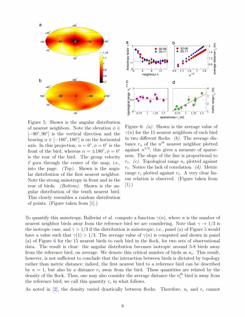
Figure 5: Shown is the angular distributionof nearest neighbors. Note the elevation ϕ ∈[−90◦, 90◦] is the vertical direction and thebearing α ∈ [−180◦, 180◦] is on the horizontalaxis. In this projection, α = 0◦, ϕ = 0◦ is thefront of the bird, whereas α = ±180◦, ϕ = 0◦

is the rear of the bird. The group velocityv goes through the center of the map, i.e.,into the page. (Top). Shown is the angu-lar distribution of the first nearest neighbor.Note the strong anisotropy in front and in therear of birds. (Bottom). Shown is the an-gular distribution of the tenth nearest bird.This closely resembles a random distributionof points. (Figure taken from [1].)

Figure 6: (a). Shown is the average value ofγ(n) for the 15 nearest neighbors of each birdin two different flocks. (b). The average dis-tance rn of the nth nearest neighbor plottedagainst n1/3; this gives a measure of sparse-ness. The slope of the line is proportional tor1. (c). Topological range nc plotted againstr1. Notice the lack of correlation. (d). Metricrange rc plotted against r1. A very clear lin-ear relation is observed. (Figure taken from[1].)

To quantify this anisotropy, Ballerini et al. compute a function γ(n), where n is the number ofnearest neighbor birds away from the reference bird we are considering. Note that γ → 1/3 isthe isotropic case, and γ > 1/3 if the distribution is anisotropic; i.e., panel (a) of Figure 5 wouldhave a value such that γ(1) > 1/3. The average value of γ(n) is computed and shown in panel(a) of Figure 6 for the 15 nearest birds to each bird in the flock, for two sets of observationaldata. The result is clear: the angular distribution becomes isotropic around 5-8 birds awayfrom the reference bird, on average. We denote this critical number of birds as nc. This result,however, is not sufficient to conclude that the interaction between birds is dictated by topologyrather than metric distance; indeed, the first nearest bird to a reference bird can be describedby n = 1, but also by a distance r1 away from the bird. These quantities are related by thedensity of the flock. Thus, one may also consider the average distance the nth

c bird is away fromthe reference bird; we call this quantity rc in what follows.

As noted in [2], the density varied drastically between flocks. Therefore, nc and rc cannot

8

remain constant for every set of data; if the interaction between birds is truly dependent onmetric distance, rc is constant, and therefore in a small density flock, nc would be small, sinceless birds would be inside a given reference bird’s “domain of influence.” Conversely, if theinteraction between birds is dependent on topological distance nc, then for a low density flock,rc should get large, as birds farther away in metric distance from a given reference bird will stillinfluence the reference bird. The inverse of the above statements is true for high density flocks.

To determine whether it is the metric or topological distance that dictates the interaction be-tween birds, Ballerini et al. compute nc and rc as functions of density [1]. To do this in aquantitative way, Ballerini et al. note that the amount of birds inside a ball of radius r is givenby n1/3 ∼ r/r1, where r1 is the average distance between a reference bird and its first nearestneighbor, which can be inferred from the data, see Figure 6(b). The critical relations are givenby the same equation, i.e., n1/3

c ∼ rc/r1. In the metric distance scenario, rc is constant, andthus we expect a linear relationship between n−1/3

c ∼ r1. On the other hand, in the topologicalscenario, nc is constant, and so we expect that r1 ∼ rc, see Figure 6(c) and (d) for results. It isfound that there is no significant correlation between n−1/3

c and r1, but there is significant corre-lation between r1 and rc, thus strongly supporting the argument that the underlying interactionin bird flocking is topological, not dictated by metric distance [1].

Figure 7: Shown is the probability distributionof the number of connected components of aflock after being subjected to a perturbationmodeled after a predator. (Figure taken from[1].)

Ballerini et al. further support this hypothesisvia numerical experiments. They note that, infield observations of flocking, flocking behavioris robust, often not splitting into more than 2or 3 separate units under perturbations [1, 2].They therefore simulate both the Vicsek model[11] in the parameter range where flocking oc-curs and an alternative Vicsek model, wherethe interaction is topological rather than met-ric, under a perturbation meant to model apredator. After Monte Carlo simulation overnumerous parameter values, the probabilitythat the flock is broken up into a number ofunits M is displayed by Figure 7. Clearly, Bal-lerini et al. conclude, topological interactionsare more stable under perturbations than metric distance based models, further supporting theirfindings from data analysis. In the next section, we discuss a model that involve topologicalinteractions, as supported by the above considerations.

5 Topological models of flocking

In 2012, a model put forth by Bialek et al. was formulated to agree with the observationalfindings in [1, 2] that relied on no modeling assumptions; it relies only on the principle ofmaximum entropy [3]. The model is constructed as follows. Consider a flock of N birds. Toeach bird, we attach a velocity vi, which is normalized such that si := vi/|vi|. Bialek et al.follow the hypothesis that flocks admit stationary states, which implies that the velocities sican be drawn from a probability distribution P ({si}). However, they cannot infer P ({si}) fromexperimental data; instead, they infer the matrix of correlations between normalized velocities

9

Cij := ⟨si · sj⟩. They then choose the probability distribution P ({si}) that is as random as itcan be while still matching experimental data, i.e., the distribution with maximum entropy [3].The probability distribution is therefore given by

P ({si}) =1

Z({Jij})exp

(1

2

N∑i=1

N∑j=1

Jij si · sj

), (5.1)

where Z({Jij}) is the partition function and Jij is the interaction strength that corresponds toCij. Bialek et al. use

⟨si · sj⟩P = ⟨si · sj⟩experiment, (5.2)

to match Jij to the experimentally determined Cij. It is interesting to note that the model putforth by (5.1) is exactly equivalent to the Heisenberg model of magnetic systems, with kBT = 1.As in most physical systems, once the Hamiltonian is determined, Langevin dynamics describethe plausible dynamics of relaxing towards equilibrium, given by

dsidt

= −∂H

∂si+ ηi(t) =

N∑j=1

Jij sj + ηi(t), (5.3)

where ηi(t) is a white noise term. Finding trajectories that solve (5.3) produces trajectories thatare drawn from (5.1) [3].

Bialek et al. incorporate the findings of [1, 2] by allowing the interaction strength to be in-dependent of the bird’s identity, which sets the interaction strength J > 0 to a constant, andallowing a given bird to only interact with its nc nearest neighbors. This simplifies (5.1) to

P ({si}) =1

Z(J, nc)exp

J

2

N∑i=1

∑j∈ni

c

si · sj

, (5.4)

where j ∈ nic means that bird j belongs to the set of nearest neighbors for bird i. Note this

simplification also simplifies the calculation of the correlation, which also becomes a constant,and is given by

Cint =1

N

N∑i=1

1

nc

∑j∈ni

c

⟨si · sj⟩ ≈1

N

N∑i=1

1

nc

∑j∈ni

c

si · sj. (5.5)

A summary of the results found in [3] is as follows. First, they compute the correlation Cint

predicted by the model via equation (5.5) as a function of J and compare it to the experimentalvalue of correlation, see Figure 8(a); using Cint(J, nc) = Cexp

int , they determine J(nc). Usingprobability data as a function of nc, they fix nc as the value where the log likelihood is maximized;this then fixes nc and J in the maximum entropy state, see Figure 8(b). This procedure isrepeated for all flocks, and the mean and standard deviation is computed over time.

In Figure 8(c) and (d), the values of J and nc are computed as a function of the flock’s spatialsize, L, respectively. Note that [3] do not report any trend in the values of J or nc as a functionof the flock size. The result for nc agrees with the findings of [1]; since nc is constant, it doesnot matter whether a pair of birds are separated by 1 m or 5 m, so long as they are sufficientlyclose to each other in topological distance.

10

Figure 8: (a). Estimation of Cint as a function of J with nc = 11. (b). The log-likelihood of thedata per bird (⟨P ({si})⟩exp/N)as a function of nc with J optimized for each nc. Maximum is atnc ≈ 11. (c). Inferred value of J as a function of flock size, averaged over all snapshots of thesame flock. (d). As in (c), but for nc. (e). Inferred value of the topological range n−1/3

c againstsparesness r1. (f). As in (e), but for metric range rc. (Figure taken from [3].)

The last two panels of Figure 8, panels (e) and (f), test the same hypothesis as [1] involvingcorrelations between nc, r1, and rc, where r1 is the sparesness and rc is the critical metricdistance of a given bird’s “domain of influence,” see §4 for a detailed overview of the arguments.In short, [3] finds no linear correlation between n−1/3

c ∼ r1, yet finds significant linear correlationbetween rc ∼ r1, thus affirming the hypothesis that the interactions in bird flocks are determinedby topological distance rather than metric distance.

The results presented in [3] agree well with those found in [1], however, Bialek et al. overes-timate the topological interaction distance nc by about 5 birds compared to [1]. Even withthis numerical difference, qualitatively, the model proposed in [3] predicts the propagation ofdirectional order throughout the flock with no tunable free parameters. Additionally, it predictslong range, scale free correlations between pairs of birds, as well as local effects. It is emphasizedagain that this model is formulated on a fundamentally different set of axioms than what wasused to postulate the models in §2 and §3, and reproduces similar flocking behavior using thegeneral principle of entropy maximization. Furthermore, the axioms of Bialek et al. are wellmotivated by observations [1, 2], making this theory promising for future investigation into thenature of bird flocking.

6 Summary

In this work, we present the myriad of ways that scientists have investigated bird flocking acrossdisciplines. In computational science, we discussed how the first numerical simulations of birdflocking were carried out, and the set of rules enforced on the simulated agents. We similarlydiscussed early theoretical models, namely the Vicsek model of flocking, and its framework forstudying flocking, including the discovery of a phase transition. Recent alterations made to the

11

Vicsek models find the type of phase transition occurring within the model changes if you limitthe amount of information a given bird perceives from its environment. The weakness of theabove approaches is that their assumptions, while intuitive, are not supported by observationaldata. We then summarize the findings of observational studies, and how these studies challengedthe assumptions of the Vicsek model and early numerical models. Finally, we close with anexploration of an updated model of bird flocking, containing no free parameters, that is based offof observational data. This model is found to agree well with the data used in the aforementionedobservational study.

References

[1] M. Ballerini, N. Cabibbo, R. Candelier, A. Cavagna, E. Cisbani, I. Giardina, V. Lecomte,A. Orlandi, G. Parisi, A. Procaccini, M. Viale, and V. Zdravkovic. Interaction ruling animalcollective behavior depends on topological rather than metric distance: Evidence from afield study. Proceedings of the National Academy of Sciences, 105(4):1232–1237, 2008.

[2] M. Ballerini, N. Cabibbo, R. Candelier, A. Cavagna, E. Cisbani, I. Giardina, A. Orlandi,G. Parisi, A. Procaccini, M. Viale, and V. Zdravkovic. Empirical investigation of starlingflocks: a benchmark study in collective animal behaviour. Animal Behaviour, 76(1):201–215, 2008.

[3] W. Bialek, A. Cavagna, I. Giardina, T. Mora, E. Silvestri, M. Viale, and A. M. Walczak.Statistical mechanics for natural flocks of birds. Proceedings of the National Academy ofSciences, 109(13):4786–4791, 2012.

[4] A. Cavagna, I. Giardina, A. Orlandi, G. Parisi, A. Procaccini, M. Viale, and V. Zdravkovic.The starflag handbook on collective animal behaviour: Part i, empirical methods, 2008.

[5] J. A. De Loera, J. Rambau, and F. Santos. Triangulations: Structures for Algorithms andApplications. Springer Publishing Company, Incorporated, 1st edition, 2010.

[6] M. Durve and A. Sayeed. First-order phase transition in a model of self-propelled particleswith variable angular range of interaction. Phys. Rev. E, 93:052115, May 2016.

[7] H. Edelsbrunner and E. P. Mucke. Three-dimensional alpha shapes. ACM Trans. Graph.,13(1):4372, Jan. 1994.

[8] F. Heppner and U. Grenander. Ubiquity of chaos, chapter a stochastic nonlinear model forcoordinated bird flocks. The Ubiquity of Chaos, Chapter A Stochastic Nonlinear Model forCoordinated Bird Flocks, pages 233–238, 01 1990.

[9] R. Miller and W. J. Stephen. Spatial relationships in flocks of sandhill cranes (grus canaden-sis). Ecology, 47:323–327, 1966.

[10] C. W. Reynolds. Flocks, herds and schools: A distributed behavioral model. SIGGRAPHComput. Graph., 21(4):2534, Aug. 1987.

[11] T. Vicsek, A. Czirk, E. Ben-Jacob, I. Cohen, and O. Shochet. Novel type of phase transitionin a system of self-driven particles. Physical Review Letters, 75(6):12261229, Aug 1995.

12